Kinetic and hydrodynamic regimes in multi-particle-collision dynamics
of a one-dimensional fluid with thermal walls

Abstract

We study the non-equilibrium steady-states of a one-dimensional ($1D1V$) fluid in a finite space region of length $L$. Particles interact among themselves by multi-particle collisions and are in contact with two thermal-wall heat reservoirs, located at the boundaries of the region. After an initial ballistic regime, we find a crossover from a normal (kinetic) transport regime to an anomalous (hydrodynamic) one, above a characteristic size $L_{*}$. We argue that $L_{*}$ is proportional to the cube of the collision time among particles. Motivated by the physics of emissive divertors in fusion plasma, we consider the more general case of thermal walls injecting particles with given average (non-thermal) velocity. For fast and relatively cold particles, short systems fail to establish local equilibrium and display non-Maxwellian distributions of velocities.

I Introduction

Statistical systems driven away from equilibrium by external agents, like concentration and/or thermal gradients, forced flows etc. are ubiquitous in nature and in technological applications. Especially in far-from-equilibrium regimes simulation of model systems is a basic tool to gain insight on the fundamental properties of the system under study. Molecular dynamics is the most natural approach, but methods based on effective stochastic processes may be a computationally convenient alternative. In particular, the Multi-Particle Collision (MPC) dynamics can be considered as a mesoscale simulation method where particles undergo stochastic collisions. The implementation was originally proposed by Malevanets and Kapral Malevanets and Kapral (1999); Kapral (2008) and consists of two distinct stages: a free streaming and a collision one. Collisions occur at fixed discrete time intervals, and space is discretized into cells that define the collision range. The MPC dynamics is a useful tool to investigate concrete systems like polymers in solution, colloidal fluids etc. but also to address fundamental problems in statistical physics and in particular the effect of external sources.

In the present work, we investigate the transport property of a one-dimensional gas driven off-equilibrium by different reservoirs, modeled as thermal walls. This general setup has been considered very often in the literature(Lepri et al., 2003a; Dhar, 2008) with several possible applications (Lepri, 2016). For the discussion that follows, it is worth recalling that the prediction of Nonlinear Fluctuating Hydrodynamics van Beijeren (2012); Spohn (2014) for 1D systems, constrained by three global conservation laws, is that transport is generically anomalous and belongs to the Kardar-Parisi-Zhang (KPZ) dynamical universality class. This is confirmed by other approaches including hydroynamics Narayan and Ramaswamy (2002); Delfini et al. (2006), kinetic theory Pereverzev (2003); Nickel (2007); Lukkarinen and Spohn (2008) and many numerical simulations Lepri et al. (2003b); Wang and Wang (2011); Liu et al. (2014). However, for finite systems some deviations are found and it is thus of interest to clarify which are the different transport regimes (see e.g. Refs.Benenti et al. (2020); Lepri et al. (2020) for an up-to-date account). In this framework, simple kinetic model are an unvaluable testbed.

Besides the general theoretical motivations, our interest in also in application of the technique in plasma physics Di Cintio et al. (2015, 2017). We wish to investigate the MPC method as a tool to study nonequilibrium properties of fusion plasma which are subject to large temperature gradients. This is a relevant issue in the modeling of plasma transport in the direction parallel to the magnetic field in the edge of magnetic fusion devices where hot plasma regions are connected to a wall component. In this case a significant temperature gradient along the field line sets in between the hot region, that acts as a heat source, and the colder plasma region at the wall, that acts as a sink. Deviations from the classical Fourier law have been observed (see for example Stangeby (2000); Krasheninnikov et al. (2020) and references therein) together with transitions from strongly collisional to collisionless regimes, exhibiting different heat conduction features. We want to point out that accounting for these kinetic effects by a fluid model of heat transport is of primary importance for implementing realistic and efficient hydrodynamic simulations. In this perspective, what contained in this work can be considered as a worthwhile evolution along the line of simplified 1D fluid models, already adopted for studying thermal transport in plasmas Bond (1981); Bufferand et al. (2010, 2013). For the sake of brevity, we adopt for such model the label $1D1V$ used sometimes in the literature, meaning that we consider particles constrained on the line with one velocity component along it.

Besides this, in the edge plasma of magnetic fusion devices several phenomena, like for example neutral beam injection are related with the injection of hot and/or cold plasma particles. We refer for example to hot sources related to external heating of the plasma but also to particular regimes with emissive divertor targets on the wall due to the high temperatures associated with steady state loads, as expected for example on next step large fusion devices Kocan et al. (2015); Gunn et al. (2017). Here, we will thus attempt to model this situation, by generalizing the usual thermal wall method to include the possibility of injecting particles with an average non-thermal velocity. To our knowledge this case has not been treated in the statistical physics literature and it has thus an interest by itself.

The outline is as follows. In Section II we recall the definition of the fluid dynamics and the thermal walls. Section III discusses the crossover from the so called kinetic (diffusive) regime to the anomalous, hydrodynamic one. The effect of general thermal walls is illustrated in Sec. IV with reference to the specific case of shifted Maxwell-Boltzmann distributions.

II 1D1V MPC with thermal walls

For a detailed description of the MPC simulation scheme we address the reader to references Di Cintio et al. (2015, 2017). Here, we just summarize the basic ingredients. We consider an ensemble of $N$ point particles with equal masses $m$ located in a finite space region, $[0,L]$, partitioned into $N_{c}$ (fixed) cells of size $a$, $L=N_{c}a$. The density of particles, $d=N/L$, is fixed, while all physical quantities, without prejudice of generality, are set to dimensionless units, namely $a=1$, $m=1$ and (for the isolated system) $E_{c}=1$, the latter denoting the total kinetic energy of the fluid of particles.

The MPC collision is performed at regular times steps, separated by a constant time interval of duration $\delta t$: the velocity of the $j$-th particle in the $i$-th cell is changed according to the update rule $v_{j,{\rm old}}\to v_{j,{\rm new}}=a_{i}w_{j}+b_{i}$, where $w_{j}$ is randomly sampled by a thermal distribution at the cell temperature $T_{i}$, while $a_{i}$ and $b_{i}$ are cell-dependent parameters, determined by the condition of total momentum and total energy conservation in the cell Di Cintio et al. (2015). After the collision all particles freely propagate, i.e.

$$x_{j}(t+\delta t)=x_{j}(t)+v_{j}(t)\,\delta t\,.$$ (1)

and they may move to a new cell.

The non-equilibrium state is imposed by two thermal walls Tehver et al. (1998) acting at the edges of the space region: any particle crossing the boundaries of the interval $[0,L]$ is re-injected in the opposite direction with a random velocity extracted form the Maxwell-Boltzmann distributions

$$p_{0}(v)=\frac{v}{T_{0}}e^{-v^{2}/2T_{0}};\quad p_{L}(v)=-\frac{v}{T_{L}}e^{-v^{2}/2T_{L}}\,.$$ (2)

Re-injected particles propagate with their new velocities for the remaining time up to the next collision. Since arbitrarily large values of $v$ are admitted, a particle may reach the opposite boundary during this time, although such a process, in practice, becomes extremely unlikely, i.e. negligible, for sufficiently large values of $L$, considering that in the adopted dimensionless units the typical value of $v$ is ${\mathcal{O}}(1)$.

The heat fluxes at the two boundaries, $Q_{0}$ and $Q_{L}$, respectively, are computed as the average kinetic energy exchanged by particles interacting with the walls Lepri et al. (2003a); Dhar (2008). The relaxation of the fluid to a steady state, i.e. $Q_{0}\approx-Q_{L}=Q$, is monitored by controlling the convergence of the running-time averages of the fluxes. The thermal conductivity is defined as $K=Q/(\Delta T/L)$, where $\Delta T=T_{0}-T_{L}$. Typically, in order to speed up the relaxation to a steady state, the initial velocities of the particles in cell $i$ are randomly extracted from a Maxwell-Boltzmann distribution at temperature $T_{i}=T_{L}+(T_{0}-T_{L})i/L$, i.e. according to the linear temperature profile compatible with the Fourier’s law.

The relevant kinetic parameters of the MPC protocol are the particle mean free path $\ell$, which, in an uniform system, is proportional to the thermal velocity of the fluid $v_{T}=\sqrt{T}$, in formulae $\ell\sim v_{T}\delta t\,,$ and the thermal conductivity, that is expected to be proportional to the typical kinetic energy of the fluid, in formulae $K=Cv_{T}\ell\sim v_{T}^{2}\delta t$, $C$ being the specific heat at constant volume.

We conclude this section by making the reader aware of the main advantage of MPC simulations, with respect to those typically performed in nonlinear lattice models. The possibility of observing crossover between different transport regimes in the latter class of models depends on the fine tuning of various simulation parameters, e.g. energy density, integration time step, coupling with the thermal reservoirs, and all that are strongly model-dependent, because the crossover effects are ruled by the lifetime of typical nonlinear excitations, influencing the stationary transport process. As we show in what follows, in MPC simulations one can control different regimes essentially by a single natural parameter, the collision time $\delta t$, which is straightforwardly related to the mean-free path of the fluid particles, weak and strong collisional regimes corresponding to large and small values of $\delta t$, respectively.

III From kinetic to hydrodynamic regimes

The kind of stationary heat transport phenomenon one is dealing with is characterized by the scaling of $Q$ with the system size $L$. Diffusive transport, i.e. Fourier’s law, yields $Q\propto L^{-1}$. For the $1D1V$ MPC, based on general theoretical arguments van Beijeren (2012); Spohn (2014) we expect that transport would be anomalous and belonging to the KPZ universality class, as indicated by equilibrium correlation functions (Di Cintio et al., 2015). In the nonequilibrium setup used in the present work this would imply that

$$Q\propto L^{-2/3}\qquad L\to\infty\,.$$ (3)

However, this asymptotic anomalous regime may be eventually attained going through a crossover from a standard kinetic, i.e. diffusive, regime Zhao and Wang (2018); Miron et al. (2019); Lepri et al. (2020). This scenario can be rationalized by assuming that the flux is made of two contributions

$$Q=Q_{N}+Q_{A}\,,$$ (4)

where $Q_{N}$ is the ”normal” part of the flux that can be written as

$$Q_{N}=\frac{q}{r+L/\ell}$$ (5)

(with $q$ and $r$ being suitable parameters) while $Q_{A}$ is the anomalous part that, for large enough values of $L$, should scale as

$$Q_{A}\sim\left(\frac{b}{L}\right)^{\frac{2}{3}}\,,$$ (6)

and $b\sim{\mathcal{O}}(1)$ is a characteristic length Lepri et al. (2020). Formula (5) is suggested by kinetic theory to account for the crossover from initial ballistic regime to a diffusive one, see e.g. Ref. (Aoki and Kusnezov, 2001) and Section 3.4 in Ref. (Lepri et al., 2003a). It implies that up to system lengths of the order of the mean free path $L\sim\ell$ transport is essentially ballistic, with a flux independent of $L$ while for $L\gg\ell$, $Q_{N}\sim\frac{\ell}{L}$.

According to the above formulae, for large enough $L$ one can define a crossover length $L_{*}$ from the normal to the anomalous regime when $Q_{N}\approx Q_{A}$, i.e.

$$L_{*}\sim\left(\frac{\ell^{3}}{b^{2}}\right)\sim v_{T}^{3}\,\delta t^{3}.$$ (7)

Altogether, upon increasing $L$ at fixed $\ell$, one should see a first ballistic regime followed by a kinetic (diffusive) one until eventually the asymptotic hydrodynamic regime is attained. It should be however remarked, that the different regimes are observable only provided that the relevant length scale are widely separated, in such a way that the range of scales between the ballistic and anomalous regimes is large enough i.e. $\ell\ll L_{*}$.

The numerical results reported in Fig.1(a) provide a clear confirmation of this scenario. The energy flux $Q(L)$ displays a crossover from diffusive to anomalous scaling upon decreasing the collision time $\delta t$. In Fig.1(b) we also show that, for low collisionality and small $L$, the thermal conductivity $K$, obtained for different values of $\delta t$, tend to collapse onto a single curve after rescaling $K$ and $L$ by $\delta t$, or, equivalently, by $\ell$ . This confirms that in the kinetic regime $\ell$ is the only relevant scale as expected.

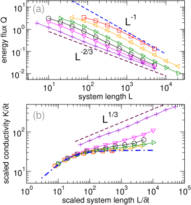
Figure 1: Simulations of MPC fluid with density $d=5$, $T_{0}=4$, $T_{L}=2$. (a) Scaling of the energy fluxes $Q$ as a function of the size $L$ for increasing collision times $\delta t=0.1,0.5,1.0,2.0,5.0$ and $10$ (bottom to top); the upper and the lower dashed lines correspond to the scaling of normal and anomalous transport, respectively. (b) Scaling of the heat conductivity $K=QL/\Delta T$ with the system size $L$; the dot-dashed blue line is a fit of the data with $\delta t=10$ with the functional form $34.2x/(12.2+x)$, see Eq.(56) in Ref.Lepri et al. (2003a)

.

A more refined analysis of the data, supporting Ansatz (4), can be obtained by estimating the two contributions in Eq.(4). This is accomplished by fitting rescaled conductivity data with the largest $\delta t$ via the functional form $\frac{AL}{B+L}$ suggested by Eq. (5), with $A,B$ being fitting parameters.

As seen in Fig.1(b) (dash-dotted line) the fitting is very accurate meaning that the anomalous contribution to the conductivity is negligible over the considered length range. From the fitting function, one can obtain straightforwardly the best estimate of $Q_{N}$ and thus the anomalous part as $Q_{A}=Q-Q_{N}$. As shown in Fig.2, a power law fit of $Q_{A}$ indicates an excellent agreement with the expected scaling Eq.(3) on a remarkably large range of about three decades in $L$. To our knowledge, this one of the most solid numerical confirmations of the predictions of fluctuating hydrodynamics. We also note, that the characteristic length $b$ is found to be independent of the collision parameter.

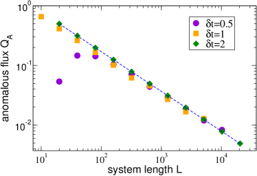
Figure 2: Scaling of the anomalous component of the energy currents $Q_{A}$ for $d=5$, $T_{0}=4$, $T_{L}=2$ and different collision times. The flux $Q_{A}$ is computed subtracting the normal component $Q_{A}$ as detailed in the text. The dashed line is a best-fit of the data with $\delta t=2$, yielding a decay $Q_{A}\propto L^{-0.66(5)}$.

The difference between the two regimes can be further appreciated also in the temperature and density profiles computed as averages of $v_{i}^{2}$ and of the number of particles in each one of the $N_{c}$ cells. In order to deal properly with the large $L$ limit, we plot the temperature and the density profiles, $T(x)$ and $n(x)$, respectively, as a function of rescaled variable $x=i/L$, where $i$ is the cell index. This representation allows one to conclude also that local equilibrium is attained, since the product $T(x)n(x)$ is $x$-independent, as expected for an ideal gas (data not shown).

In Fig.3 we report these profiles for two different values of the collision time and different sizes $L$. For $L<L_{*}$ the temperature profiles are in good agreement with the prediction of Fourier’s law, with thermal conductivity given by the kinetic theory, namely $K(T)\propto T$. In fact, solving the stationary heat equation $(K(T)T^{\prime})^{\prime}=0$ on the domain $[0,L]$ with imposed boundary temperature $T(0)=T_{0}$ and $T(1)=T_{L}$ one obtains

$$T(x)=\left[T_{L}^{2}+(T_{0}^{2}-T_{L}^{2})x\right]^{1/2}.$$ (8)

As shown in Fig.3(a) this functional form accounts for the measured shapes for large enough $L$, apart the temperature jumps at the edges, that are a typical manifestation of boundary impedance effects. A similar situation was found also for the HPG model Dhar (2001); Grassberger et al. (2002). Also, considerations of the same type apply to the density profiles in Fig.3(b), in view of the relation $T(x)n(x)\approx constant$.

In the hydrodynamic regime, i.e. $L>L_{*}$, the temperature profiles exhibit instead the typical signatures of anomalous transport, signaled by singularities at the boundaries (see Fig.3(c,d)). For instance, the inset in Fig.3(c) shows that $T(x)\sim(1-x)^{\mu}$ for $x\to 1$. This property is traced back to the fact that steady state profiles should satisfy a fractional heat equation (Lepri and Politi, 2011). The parameter $\mu$ has been termed meniscus exponent $\mu$, as it described the characteristic curvature close to the edges. In the simulations here $\mu\approx 3/4$, a value already found for other models with reflecting boundary conditions Lepri and Politi (2011); Kundu et al. (2019).

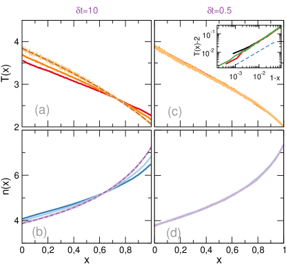
Figure 3: Simulations of MPC fluid with density $d=5$, $T_{0}=4$, $T_{L}=2$. Kinetic regime ($\delta t=10$): temperature (a) and density (b) profiles for $L=160,320,1280$ (bottom to top); dashed lines are fits with the function in Eq.(8) yielding $T_{0}=3.9$, $T_{L}=2.0$. Hydrodynamic ($\delta t=0.5$) regime: temperature (c) and density (d) profiles for $L=640,1280,2560$; the inset in panel (c) shows the singularity at the right edge of the temperature profile, the dashed line corresponding to a power-law behavior $T(x)\sim(1-x)^{3/4}$ (see text for details).

IV General thermal walls

Having in mind the possibility of simulating the injection of hot and/or cold particles into a fusion plasma by the MPC protocol, in this Section we describe how one can cope with this task by introducing suitable and more general boundary conditions. Within the adopted thermal wall scheme this can be achieved by changing the distributions of re-injected particles at one boundary of the space region. For instance, it can be assumed that the distribution $p_{0}$ on the left boundary is replaced by a function of the general form Ianiro and Lebowitz (1985)

$$p_{0}=vH(v)\quad.$$

By imposing the condition $\int_{0}^{\infty}vH(v)dv=1$, we ensure that the net flux of particles vanishes Ianiro and Lebowitz (1985). This distribution can be characterized by two parameters, namely the typical average velocity of the injected particles

$$v_{0}=\int_{0}^{\infty}v^{2}H(v)dv$$

and the typical velocity variance

$$(\Delta v)^{2}=\int_{0}^{\infty}v^{3}H(v)dv-v_{0}^{2}\,,$$

that measures the source spread .

As a specific example, here we consider a shifted Maxwellian distribution

$$H(v)=H_{0}(V)e^{-(v-V)^{2}/2T_{0}}\,,$$ (9)

parametrized by the velocity $V$, where $H_{0}$ is a suitable normalization factor. Shifted Maxwellian sources are implemented in kinetic models to account for drift speed of plasmas Gunn (2005). Manifestly, both $v_{0}$ and $\Delta v$ are functions of $V$ and $T_{0}$. In the following simulations, we generate random velocities drawn from (9) and use $V$ and $T_{0}$ as control parameters, reporting also the corresponding values of $v_{0}$ and $\Delta v$ for comparison .

In Fig.4 we present the results of MPC simulations for different values of $\delta t$ and $V$. We first of all note that, even setting equal temperatures at the thermal walls, i.e. $T_{0}=T_{L}$, the system is out of equilibrium and there is a net flux of energy and particles. For what concerns the scaling with of the flux with the size $L$, the effect of these thermostats is pretty similar to the standard case discussed in the previous Section. As shown in Fig.4a, in the case of relatively large collisionality the anomalous scaling, Eq.(3) is attained. For weak collisionality, Fig.4b the diffusive scaling is found in the considered range. Although not observed in the data, we expect the same crossover described above beyond the hydrodynamic scale. In both cases, as expected, one observes that the magnitude of the current increases upon increasing the speed of the injected particles. The above results are not obvious, and indicate that regardless of the nature of the baths the overall scenario is mostly dictated by bulk properties.

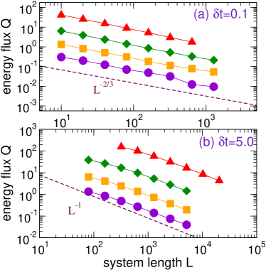
Figure 4: Simulations with thermal wall given by Eq.(9) on the left-hand boundary for different values of the parameter $V$, $T_{0}=T_{L}=3$ $d=5$; (a) $\delta t=0.1$,(b) $\delta t=5.$ $V=1,2,4,8$ from bottom to top. The dashed lines denote the asymptotic decay corresponding to normal and anomalous transport.

To better appreciate the effect of this kind of thermal wall we measured the position-dependent steady state distributions $f(x,v)$ in phase space for a moderate collisional parameter $\delta t=10$, see Fig.5. We consider two cases:

1. the typical entry speed $v_{0}$ is of the same order of the thermal velocity $v_{0}\sim\Delta v=\sqrt{T_{0}}$ (left panels in Fig.5). In this case the situation is very similar to the standard thermal bath: temperature and density gradients are formed, while velocity distributions are Maxwellian even relatively close to the left boundary, thus indicating that local equilibrium has been achieved pretty fast.

2. fast, i.e. ”cold”, particles are injected, i.e. the typical entry speed $v_{0}$ is larger than $\Delta v$ (right panels in Fig.5). In this case one observes that the beam of particles entering from the left wall propagates, while experiencing the effect of the interactions with the cloud of almost-thermalized particles only in the center of the space region. As a result, the velocity distributions are strongly non-Maxwellian and remain double-humped in the first half of the space region.

Adopting a kinetic point of view, we expect that the typical size of the region in which the fluid is not in local equilibrium would be of the order of mean free path $\ell$. For the simulations above, we checked that upon increasing $L$ such a region remains indeed finite. On the other hand, in anomalously conducting systems lack of thermal equilibrium close to the sources is found Delfini et al. (2010) and we cannot exclude that the same occurs here for larger systems.

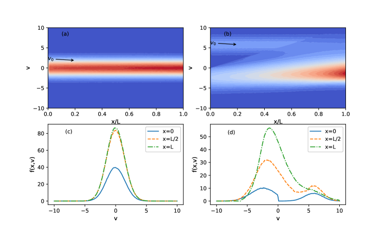
Figure 5: Simulations with thermal wall defined by Eq. (9). (a,b) Particle distributions $f(x,v)$ in the steady state and (c,d) their cuts at different positions; the arrows indicate the typical injection velocity $v_{0}$; $T_{0}=2$ $T_{L}=2$, $L=160$, density $d=5$, $\delta t=10$ Left panels (a,c): Injection of slow particles ($V=0.5$), $v_{0}=1.87$ $\Delta v=1.0$. Right panels (b,d): Injection of fast and cold particles ($V=4$), $v_{0}=5.81$ $\Delta v=1.24$ Note that even close to the right bath, $x=L$ the velocity distribution significantly deviates from a Maxwellian.

To conclude this Section, we briefly discuss the dependence of fluxes and profiles on the thermal wall parameters. In the top panel of Fig. 6 we plot the contour levels of the energy flux $Q$ as a function of $V$ and $T_{0}$ keeping the other parameters fixed. As remarked above, $Q$ increases with $V$ as intuitively expected. However there is an interesting feature occurring for small enough $T_{0}$ and $V$. For $T_{0}<T_{L}$ and $V$ small, injected particles are still relatively slow and thermalise quickly so energy mostly flows from right to left, $Q<0$. The corresponding distributions and profiles $T(x)$ and $n(x)$ are shown in the leftmost panels of Fig. 6, where it is seen that $T$ is decreasing. However, increasing the speed of the injected particles leads to a sign reversal of the current, $Q>0$ and of the associated gradients (right panels of Fig. 6). A rough estimate of the conditions where this inversion takes place, can be obtained by equating the kinetic temperature $T_{L}$ of the rightmost reservoir with (twice) of the kinetic energies of the injected particle, which roughly gives $T_{L}\approx T_{0}+V^{2}$. As seen in Fig. 6(a) this is in agreement with the numerical data. The above estimate (dashed white line) indeed separate the two regions of the parameters plane having different signs of the energy current. On the basis of this observation, one may argue that the velocity $V$ can be used as a further control parameter of the flux direction.

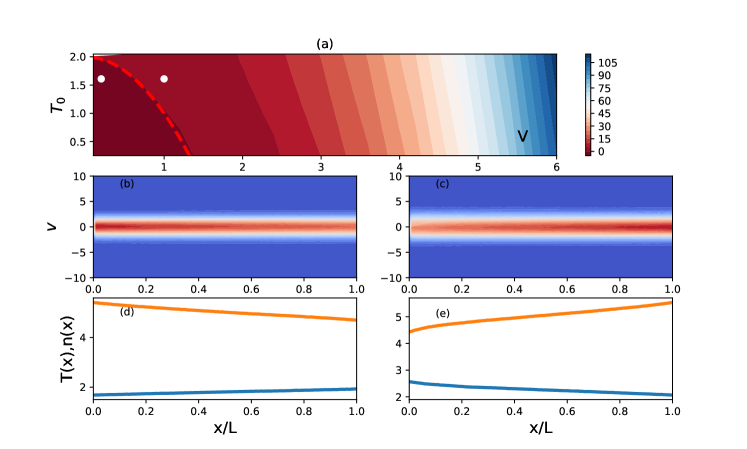
Figure 6: Energy current reversal: (a) Contour plot of the flux $Q$ as a function of the thermal wall parameters $V$ and $T_{0}$; Simulations with other parameters fixed $T_{L}=2$, $L=160$, $d=5$, $\delta t=10$. The dashed red line is the curve $T_{0}=2-V^{2}$, the energy flux is negative on the left side of it (see text for details). (b,c) the velocity distribution functions $f(x,v)$ and (d,e) temperature and density profiles (lower and upper curves respectively). Panels (b,d) and (c,e) are for the parameter values corresponding to $T_{0}=1.6$ and $V=0.2,1$ respectively (see the two white dots in the upper panel) showing change in the sign of the gradients.

V Conclusions

In this work we have considered properties of non-equilibrium steady-states and transport in a one-dimensional ($1D1V$) fluid in a finite space region of length $L$ undergoing MPC dynamics and interacting with thermal walls.

For Maxwellian walls we demonstrated a crossover from a normal (kinetic) transport regime to an anomalous (hydrodynamic) one, above a characteristic size $L_{*}$. Since $L_{*}$ grows cubically with the collision time $\delta t$, the anomalous regime may hardly be detected with the sizes typically used in simulations. So we argue that a standard diffusive description will account for the observation for short enough systems. Altogether, the results nicely fit in the general framework observed for other models Zhao and Wang (2018); Miron et al. (2019); Lepri et al. (2020). They call for a critical consideration of the usual assumptions made in kinetic theory, since memory effects and long-time tail may play a major role in predicting heat and particle transport in low-dimensions.

A natural question is whether the same scenario occurs in two dimensional fluids. Here, the expectation is that in the hydrodynamic regime anomalous transport would be associated with a logarithmic divergence of the conductivity with size. For the 2D MPC dynamics this is confirmed by equilibrium simulations Di Cintio et al. (2017). Thus in principle a similar crossover scenario should occur, although it may be hard to be observed in view of such a weak logarithmic dependence.

In the second part, we considered the more general case of thermal walls injecting particles with given average (non-thermal) velocity. We showed, that the kinetic and hydrodynamic regimes are observed confirming that transport is dominated by bulk correlations in both cases. For injection of fast and relatively cold particles, short systems fail to establish local equilibrium and display non-Maxwellian distributions of velocities. We also showed that the injection velocity may be used to control current reversal.

To conclude, let us comment on the perspective of applying the model to confined plasma. This requires considering the effect of the self-consistent electrostatic field, solution of the associated Poisson equation. As already noticed in Refs.Sano and Kitahara (2001); M. Sano and Kitahara (2011), the case of equal masses and charges in one dimension can be mapped in the so-called ding-dong model Prosen and Robnik (1992). The latter consists of a one dimensional array of identical harmonic oscillators (each one with frequency $\omega_{p}$, the plasma frequency) undergoing hard-core collisions Prosen and Robnik (1992). Non-equilibrium and transport properties of such a model have been investigated in detail Prosen and Robnik (1992); Sano and Kitahara (2001); M. Sano and Kitahara (2011) and normal diffusive transport has been demonstrated, as expected since energy remains the only conserved quantity. One may thus argue that adding MPC dynamics will not affect significantly such a property and that the hydrodynamic regime will not be present. However, for finite systems the situation may be more subtle. Actually, the field introduces another relevant time scale in the dynamics, i.e. the inverse of the plasma frequency $\omega_{p}$, associated to the collective oscillations and Langmuir waves. This time scale should be compared with the collision frequency $1/\delta t$. Generally speaking, if $\omega_{p}\delta t\ll 1$ energy transport will be driven mostly by collisions, and it is not a priori excluded that hydrodynamic effects may play a role over a relevant range of scales. Those issues deserve investigation and will be considered in the future.