TopoKnit : A Process-Oriented Representation for Modeling the Topology
of Yarns in Weft-Knitted Textiles

Abstract

Machine knitted textiles are complex multi-scale material structures increasingly important in many industries, including consumer products, architecture, composites, medical, and military. Computational modeling, simulation, and design of industrial fabrics require efficient representations of the spatial, material, and physical properties of such structures. We propose a process-oriented representation, TopoKnit, that defines a foundational data structure for representing the topology of weft-knitted textiles at the yarn scale. Process space serves as an intermediary between the machine and fabric spaces, and supports a concise, computationally efficient evaluation approach based on on-demand, near constant-time queries. In this paper, we define the properties of the process space, and design a data structure to represent it and algorithms to evaluate it. We demonstrate the effectiveness of the representation scheme by providing results of evaluations of the data structure in support of common topological operations in the fabric space.

1 Introduction

Knitting has been a technique for producing versatile textiles for over a millennium, and the knitting process was first automated with machinery in the 16th century [1]. Knitting produces fabrics with varied mechanical properties that can be shaped into many forms. Knitted textiles are increasingly important in a number of industries, including consumer products, architecture, composites, medical, and military. In order for these textiles to be widely deployed and reach their full industrial potential, computer-based modeling and simulation tools must be developed to support the design and optimization of knitted structures.

With this need in mind, we have developed a process-oriented representation for modeling the topology of yarns in weft-knitted textiles. Our initial focus has been on representing fabrics that can be manufactured by weft-knitting machines consisting of two flat beds of needles and a single yarn. Since it has been shown that the structures formed by yarns and their interactions dominate the mechanical behavior of knitted textiles [2, 3, 4, 5], TopoKnit represents these types of fabrics with yarns and the neighborhoods where they contact each other. The goal of our work is to define a low-level representation of knitted fabrics that has the properties of both completeness (i.e. capable of storing all knitted fabrics that can be manufactured from a specific set of stitches) and validity (i.e.  guaranteed to represent only physically valid states of the fabric). Additionally, the representation should support efficient query algorithms for evaluation and generation of many types of knitted structure models.

To date a variety of models have been proposed for knitted textiles, covering a spectrum of length scales from loop/stitch structures, to fabric swatches and complete garments. The focus of these models range from idealized purely geometric models of yarn paths, to mechanical models of stitches, to simulation models of fabrics and clothing. There has also been abundant work on visual models for accurately rendering textiles. This assortment of models have not always been compatible with each other nor have they provided a conceptual/theoretical foundation on which to build the consistent, robust analysis tools that are essential for evaluating manufacturability and providing predictive simulation capabilities. TopoKnit is a major step towards an approach capable of representing the topological structures needed for all such models.

Our ultimate goal is to develop a multiscale data structure that can capture the topological, geometric and mechanical properties/behaviors of knitted textiles. This yarn-level representation, where mechanical behaviors are derived from robust geometric models, which in turn are based on accurate topological structures, should support the simulation and optimization techniques that are essential for design operations that ensure manufacturability of the material. The representation should capture relationships, structures and phenomena at a variety of spatial and temporal scales. These features include yarn geometry, frictional contacts, and deformations occurring at the loop, stitch, pattern, swatch and garment levels.

As a first step toward achieving this goal we describe here a low-level representation, and associated data structure, that can be used to derive the topological relationships of the yarns in the various stitches that make up a knitted fabric manufactured on a 2-flatbed weft-knitting machine. For a given set of stitch operations, the data structure is capable of representing all fabrics produced by this class of knitting machines; thus endowing it with the property of completeness. We see this process-oriented representation, which we call TopoKnit, as providing the necessary foundation on which to build more detailed models of knitted textiles that include topology, geometry and mechanics. TopoKnit not only provides a foundational data structure that captures the fundamental primitives of knitted textiles, but it also includes a rich set of access functions that allows for queries of the features of the topological structure of the fabric. This alleviates the requirement for an explicit representation of what could be a very complex topology by performing on-demand evaluation as certain information is needed by higher-level applications. Examples of applications that require this type of efficient topological representation include simulations of electrical current, water, and heat flow through textiles [6, 7, 8].

2 Related Work

The early work on modeling knitted textiles focused primarily on defining and analyzing the geometric structure of knit stitches [9, 10, 11]. This work was remarkably done without the mathematical infrastructure of splines [12], which was not widely available until the 1970s. Much later work did utilize splines to describe the centerlines of yarn geometry in knitted materials [13, 14, 15, 16]. Follow-on research applied minimum energy analysis to determine the shape of relaxed yarn loops in individual stitches [17, 18, 19, 20], as well as larger bulk properties of plain-knitted fabrics [21, 22, 23]. This work was extended by Kyosev et al. [24] to include the compression of the yarns in the loop. Sherburn, Lin, et al. [25, 26] developed a modeling approach/system working on microscopic, mesoscopic and macroscopic scales to predict the mechanical properties of textiles. Duhovic and Bhattacharyya [27] simulated the knitting process in order to understand how each of a yarn’s deformation mechanisms contribute to the overall deformation energy/behavior of a yarn in a knitted fabric. In recent work, Knittel, Wadekar et al. [28, 29, 30, 31] investigated helicoid scaffolds as a framework within which to study the structure of knitted fabrics.

The first system to model and visualize complete knitted fabrics was developed by Meissner, Eberhardt and Strasser [32, 33]. Their system (KnitSim) accepts Stoll knitting machine commands (knit a stitch, transfer loops between beds, and rack the beds) and simulates the knitting process to produce an explicit topological representation of a knitted material. The topology consists of Bonding Points (BPs), where yarns wrap around each other, and edges, representing yarns, that connect the BPs. Yarns are defined as a linked list of BPs. By making assumptions about the length of yarns between BPs, a relaxation process is run to produce a 2D geometric layout for the fabric. Eberhardt and Weber [34] then applied Breen et al.’s particle approach [35] to simulate the draping behavior of knitted fabrics.

In ground-breaking work Kaldor et al. [36, 37] simulated complete swatches and articles of clothing consisting of knitted fabrics by modeling the geometry and physics of individual yarns in these items. The yarns in the model are defined with cubic B-spline curves surrounded by a constant radius to produce a swept surface with a circular cross-section. Yarn dynamics are dictated by both energy terms (kinetic and bending) and hard constraints to prevent yarn extension and collisions, while friction interactions, a critical component of correct yarn behavior, are approximated using a velocity filter that penalizes locally non-rigid motion. While the topological structure of the fabric is implied by yarn contacts, it is not explicitly represented in their model.

The Kaldor et al. work was extended by Yuksel et al. [38, 39] to produce Stitch Meshes, an approach to generating Kaldor-style knitted material models of clothing from polygonal models that represent the clothing’s surface. A shortcoming of this approach is that it utilizes stitches that cannot be created on a knitting machine, thus limiting its usefulness in a manufacturing setting. This project has recently been enhanced to generate graphical instructions for hand knitters [40]. Aspects of this work were utilized by Leaf et al. [41] to produce an interactive design tool for simulating swatch-level patterns for knit and woven textiles. To improve relaxation time, they employ a GPU implementation using periodic boundary conditions to simulate modeling unit cells. Stitch Meshes have also been used to model crocheted fabrics [42].

Igarashi et al. [43, 44] developed a technique for generating hand-knitting patterns from 3D models, along with an interactive design and visualization system. In related work, McCann, et al. [45, 46, 47, 48] have developed algorithms that can generate knitting machine commands based on a variety of polygonal models as input. These algorithms allow for the interactive design of 3D shapes,which can then be manufactured on a commercial knitting machine. In related work, Popescu et al.  [49] describe an approach for generating an automated knitting pattern given a 3D model, without being constrained to developable surfaces. Motivated by Narayanan et al. [46], Kaspar et al.  [50] introduce an interactive system which allows users of different skill levels to create and customize machine-knitted textiles.

Cirio et al. [51] define a topological representation of knits consisting of a limited set of stitches, in contrast to the yarn-geometry-based approach of Kaldor et al. As with the Yuksel et al. work, they incorporated stitches that are not manufacturable on knitting machines. They are able to generate geometric models for rendering from their representation and have defined simplified mechanical relationships on the topological structure that supports efficient simulation of the approximate physical behavior of their virtual knitted fabrics. Aspects of this work has recently incorporated yarn-level models to provide a more efficient computational method for detailed cloth simulations [52]. This work was extended by Sánchez et al. [53] to include simulation of stacked layers with implicit contact handling using a Eulerian-on-Lagrangian (EoL) discretization.

Similar to the Meissner et al. work, Counts [54] presents a graph-based representation aiming to approximate the 2D layout of knitted textiles. The developed algorithms use information from a simulation to generate a topological graph from a limited set of hand and machine knitting instructions. Using loops as its fundamental primitive, as well as the small set of supported stitches (knit and transfer), limits the yarn topology it can represent. The approach does offer the ability to generate machine knitting instructions from the graph, but its disadvantages include not supporting increases/decreases and more complex stitches, and requiring a simulation of the knitting process to generate the graph.

Finite Element Modeling (FEM) has been used to analyze the mechanical properties of knitted fabrics. Liu et al. [2, 3, 55] perform simulations with solid yarn-level geometric models [56], while Dinh et al. [57], Poincloux et al. [58] Liu et al. [59] and Sperl et al. [60] base simulations on a homogenized unit cell. All of these efforts simulate simple weft-knitted textiles, i.e. their virtual fabrics only consist of Knit and Purl stitches. Their approaches do not rely on an underlying topological model, which will make it difficult to extend them to more complicated knitted fabrics constructed from different types of stitches.

TopoKnit improves upon previous work by providing a general topological representation of fabrics that can be produced by flatbed weft-knitting machines with a standard set of stitches. Our work stands apart from the Kaldor et al. work, which simply modeled the geometry of the yarns in Knit and Purl stitches, without representing the underlying topology of the knitted structures. Our focus on incorporating process-based features in our model provides critical manufacturability properties not found in the Yuksel et al. and Cirio et al. work, which describe materials that cannot be manufactured on knitting machines. The McCann et al. work does not create a model of a knitted material, but instead makes assumptions about the physical size of a single stitch in order to generate knitting machine instructions that produce actual fabric.

While Meissner et al.’s topological model utilizes similar primitives as TopoKnit, with Bonding Points (BPs) (our Contact Neighborhoods (CNs)) connected by yarn edges, there are significant differences between the methods and capabilities of the two approaches. They generate a topological data structure from a limited set of low-level machine instructions, an approach that requires a simulation of the knitting process. We utilize a process-oriented approach based on higher-level stitch commands, which captures how the stitches modify an all-Knit-stitch structure and does not require a knitting simulation. Their approach is more limited than ours in that they assume that a row of BPs only interacts with the BPs from the previous row. This is clearly not the case with more complicated stitch patterns, as can been seen in some of our examples, e.g. Figures 19, 19 and 24.

Meissner et al.’s results are presented in low resolution and are difficult to interpret. Some of their results appear to be topologically incorrect, unphysical and generated from unexplained machine commands and stitching scenarios. They do not provide sufficient evidence to evaluate the correctness of their results. For example, they do not offer the input instructions and resulting topology graphs for their geometric results. Additionally, they do not provide the technical information needed to evaluate the generality and robustness of their approach, e.g. the details on how to generate the BP data structure from machine instructions.

3 Fabrication of Weft-Knitted Textiles

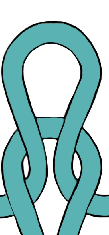
Figure 1: A single stitch, with its “legs” holding the “head” (upper loop) of the stitch below.

The loop is the fundamental structural element of knitted textiles. A new loop is formed when a yarn is drawn through a previously existing loop, as seen in Figure 1. When this process is repeated across a row, and then subsequently again in other rows, the fabric is formed [1]. When the yarn is drawn through the loop(s) held on the needle from back to front, a Knit stitch is created, as shown in Figure 3(a). A Knit stitch can be distinguished by the small “v” shapes visible on the fabric, formed by the vertical yarns of the stitches. When the yarn is drawn through the loop(s) held on the needle from front to back, a Purl stitch is created (Figure 3(b)), which is distinguishable by the horizontal sequence of small curves visible on the fabric, formed by the heads and tails of the stitches. It is important to note that Knit and Purl stitches are structurally the same, however the side from which they are viewed determines their labeling in the knitted structure.

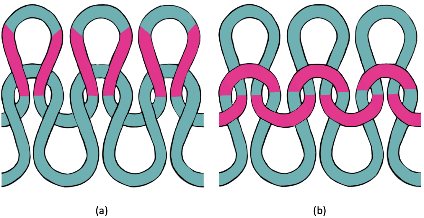
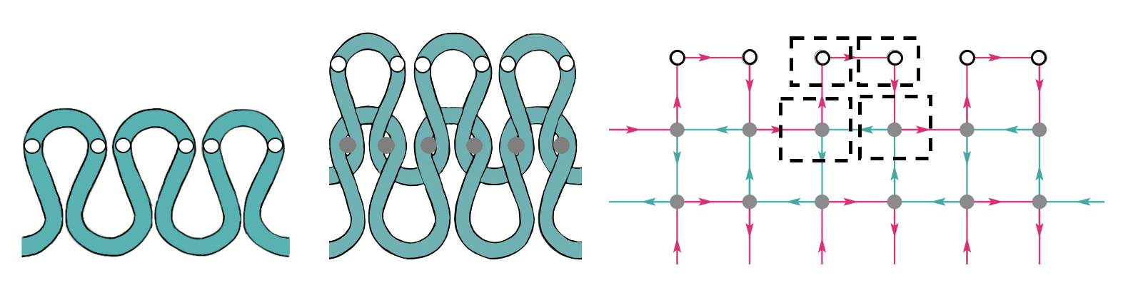
Figure 2: (a) All-Knit pattern. (b) All-Purl pattern.

          (a)               (b)                      (c)

Figure 3: A Knit stitch is created by pulling a loop of yarn through a loop held from the previous row. (a) Row of loops. (b) Knit stitches produced from another row of stitches. (c) Topological representation.

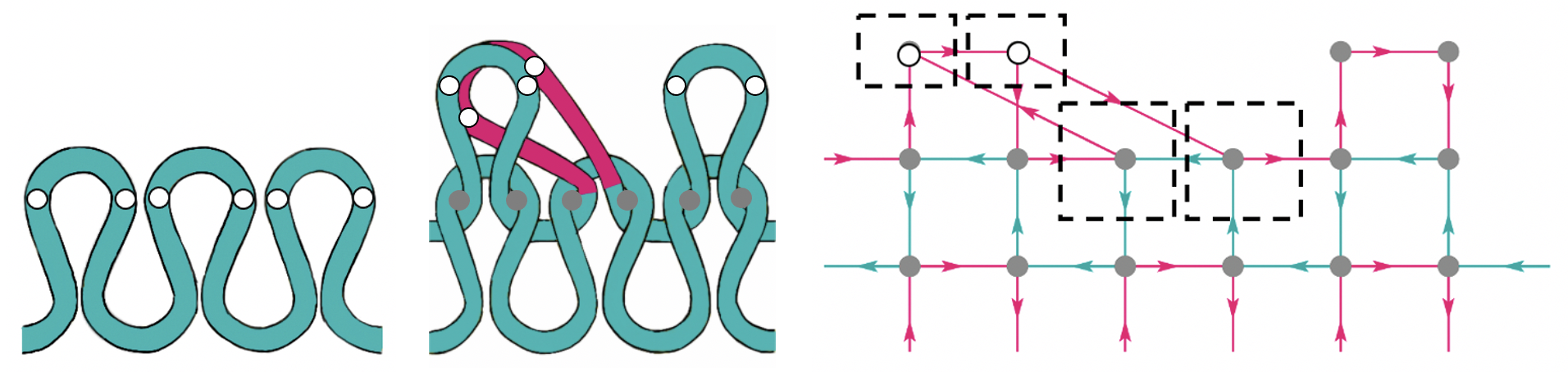
        (a)               (b)                    (c)

Figure 4: A Transfer stitch is created when the loop of a Knit or Purl stitch is transferred up to three needle positions away to the left or right.

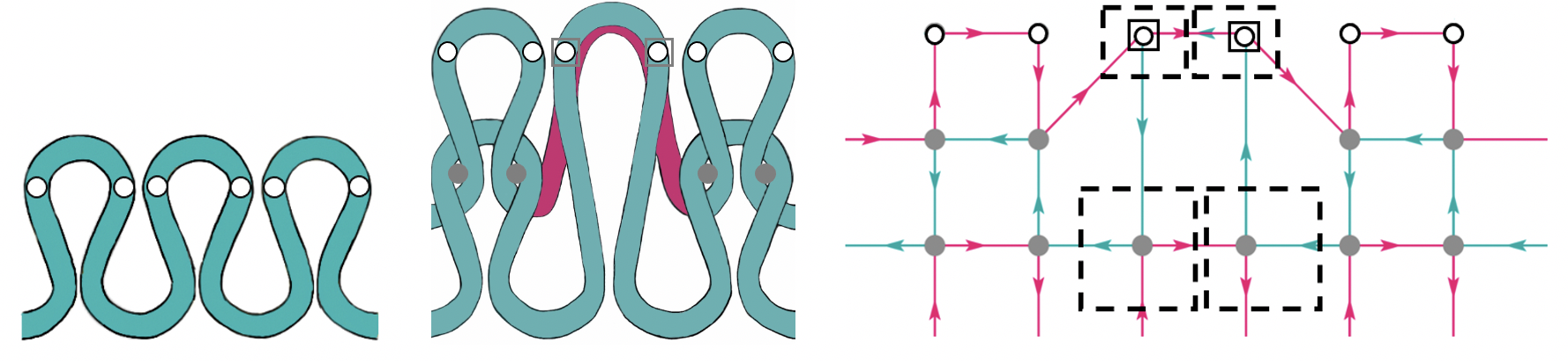
         (a)               (b)                      (c)

Figure 5: A Tuck stitch is created by tucking a yarn onto a loop held from the previous row, instead of creating a new stitch.

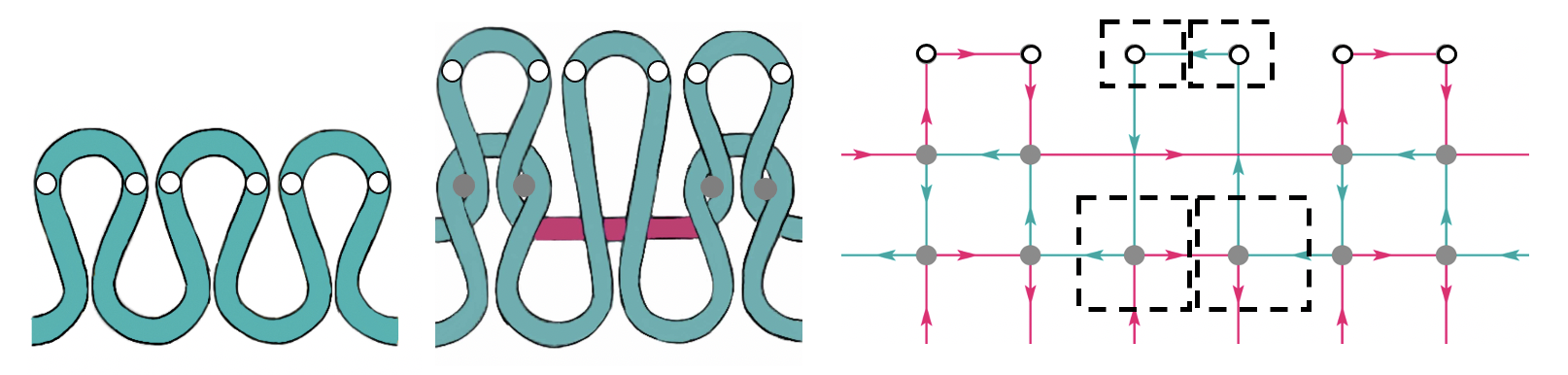
         (a)               (b)                      (c)

Figure 6: A Miss stitch is created when the needle holds a loop from a previous row as the yarn passes by, without knitting a new stitch.

Additionally, a number of other stitches can be formed, which may be combined to produce a vast variety of knitted textiles. These stitches include:
Transfer stitch
A Transfer stitch is produced when a Knit or Purl stitch is created and then its head loop is transferred, via a sequence of needle bed transfers and rackings, to another needle location. The Transfer stitch presented in Figure 4(a) transfers the loop one needle to the left, however, depending on the type of Transfer stitch there can be up to three loop movements to the left or right. When a new yarn comes to the needle holding the transferred loop, both overlapping loops will be knit together. The tranferred loop is highlighted in magenta in Figure 4(b).
Tuck stitch
A Tuck stitch is created when a yarn is tucked onto the needle and pulled up, instead of being pulled through the held loop. The tucked loop is held on the needle together with the loop from the previous row, as shown in Figure 5(a). The needle holds both loops, which will be knitted together when a stitch instruction is executed above it on the next row. The tucked loop is highlighted in magenta in Figure 5(b).
Miss stitch
Similarly to the Tuck stitch, during the execution of a Miss stitch the needle holds the loop from the previous row, but the new yarn is not hooked by the needle. Instead the yarn passes by, creating a horizontal segment of yarn across the front or the back of the held loop. The resulting horizontal yarn is highlighted in magenta in Figure 6(b).


Empty stitch
An Empty stitch specifies that no machine operation will be executed for a specific needle. Therefore, no yarn is looped on the needle at that location.

These six stitches (Knit, Purl, Tuck, Miss, Transfer and Empty) are the fundamental stitches needed to create most knitted textiles, and can be combined to generate complicated knitted patterns. TopoKnit supports all of these stitches; thus allowing for a broad representation of knitted fabrics.

4 Modeling Spaces, Primitives and Mappings

When developing a model that supports the evaluation of the validity, manufacturability and structural integrity of a particular material, it is critical to define and assess the configuration spaces associated with the material and the expressiveness of the primitives that exist within these spaces.

When modeling knitted textiles, three spaces are available for primitive definition. The first is the configuration space of the knitting machine. This would include modeling the needles, racking beds, carriages and yarn carriers of the machine, their motion and their interaction with each other and with yarns. While the advantage of this space is that it can provide information about and insight into the manufacturing process, it requires a simulation process to produce a virtual version of the material. While this approach/space can be employed to produce knitting commands for manufacturing a knitted fabric [45, 46, 47], it does not provide a representation of the material itself. Since we wish to create a representation that is machine independent and able to model materials produced on all flatbed weft-knitting machines, this space was deemed too restrictive for our purposes.

The second is the fabric space of the material itself, which is a static fully evaluated space where the structures of the manufactured fabric are directly represented. For example, a plausible topological model of any fabric could be a cell complex where 0-cells represent all contacts between yarns, oriented 1-cells correspond to yarn segments connecting adjacent contact points, and oriented 2-cells could be used to represent the yarn loops. The advantage of this space is that allows for validity checking of the fabric, for example topological correctness, but the disadvantage is that the indirect property of manufacturability is more difficult to assess and enforce. Additionally, without modeling the manufacturing process, determining the relationship between machine parameters and material characteristics is problematic. Given the nearly countless possible combinations of stitches and the complex low-level structures that these combinations can produce, it is difficult to create a single static data structure that is guaranteed to accommodate the topology and geometry of all possible fabrics. For example, representing topology of a Knit or Purl stitch may be straightforward, but the topological structure of the combination of other stitches, such as Transfer, Miss or Tuck stitches, is far less obvious.

4.1 Process Space

Our work focuses on modeling knitted textiles within a process space, an intermediate space between machine space and fabric space. This space captures aspects of both machine and fabric space, as it includes some structures of the material, as well as how those structures are manipulated by the machine during the knitting process. Process space models the abstract processes that lead to the formation of the material. In our work we focus on the processes that locally manipulate yarn loops at the stitch command level. It is the interlocking of these loops that form the central structures that hold a knitted fabric together. A contiguous block of stitches may be grouped together into swatches that can be repeated to produce a whole fabric. Additionally, the loops may be moved to other needles, both on the front and back beds of a knitting machine in order to create even more complex stitches.

The two critical components of the material that play a central role in this process are the yarn and the yarn crossings where the stitches connect with each other. Our process-oriented representation has the yarn crossing as its primary primitive, with the yarn being implicitly defined as the primitive that connects yarn crossings. The knitting process is then described as the creation and manipulation of these yarn crossings. Since the interaction of yarns at a crossing and the connections between yarn crossings may be complex, we encapsulate this complexity in a primitive we call a Contact Neighborhood (CN). This is a primitive which does not explicitly represent the geometry of the crossing yarns or the adjacencies between crossing yarns. The manipulations/movement of the CNs, for example via a Transfer stitch, are defined via mappings that change their location and possibly their state in the fabric. Thus, the topological structure (a cell complex) underlying the fabric is constructed by specifying, transforming and interconnecting CNs as explained below.

The process of knitting defines a natural bivariate parameterization of the resulting fabric. Machine weft knitting uses a row of $k$ needles. A single yarn is carried across these needles in a back-and-forth fashion. Each pass of the yarn may be labeled with integer $l$. Therefore each stitch lies in a coordinate grid and has a unique $(k,l)$ grid location. The two indices $(k,l)$ produce a parameterization over the surface of the knitted material. The definition of CNs and the way that they interconnect capture the inherent 2D topological structure of knitted textiles.

4.2 Primitives

The fabric can be described in terms of loops, but its geometric and mechanical properties are determined by lower-level components, yarns and their “contacts”, which is why we chose Contact Neighborhoods (CNs) and the yarns that connect them to be the fundamental primitives of our knitted textile data structure. Loops and stitches were deemed to be too coarse as primitives because certain stitch operations can create structures that span several needle locations and yarn rows or produce non-symmetric loops. While most loops are well-defined symmetric structures, there are cases where that symmetry is broken and the four CNs that define the loop are significantly different. Additionally, certain stitch combinations can produce complex structures that require more representational resolution than is available at the loop/stitch level.

While yarns come in many types, e.g. staple (twisted short fibers), monofilament (a single extruded material), and multifilament (twisted monofilaments), our approach assumes that the yarn, as compared to its constituent fibers, is the smallest physical element that needs to be directly modeled when simulating knitted materials. Yarns may have complex, non-linear properties, but these may be lumped without the need for modeling the individual fibers that make up the yarn. Previous work has shown that the shapes of the yarns in stitches play a significant role in the overall mechanical behavior of knitted materials [2, 3], irrespective of the deformation properties of the yarns. Therefore we chose the yarn as the lowest-level primitive to provide the connection between CNs.

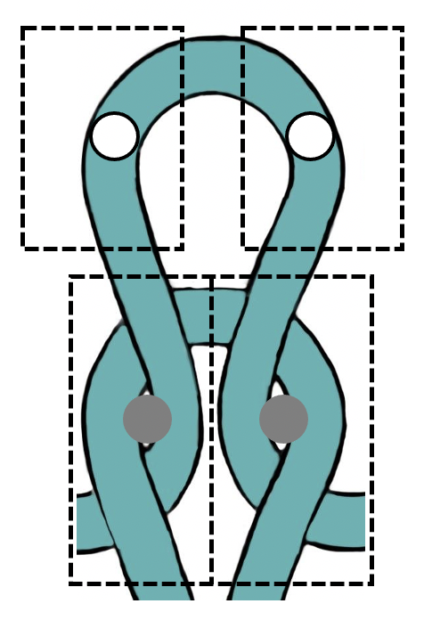
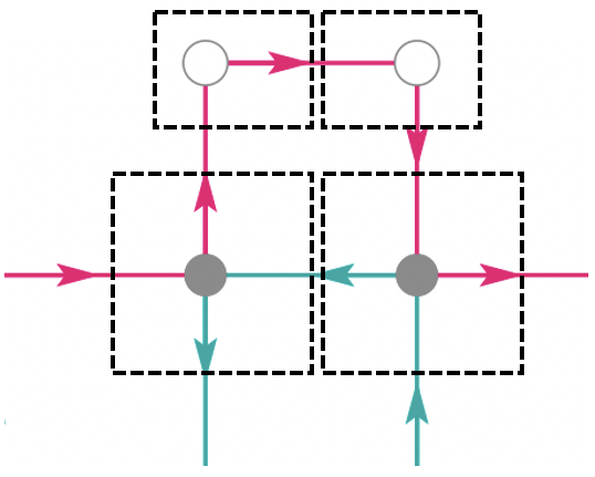
(a)                                 (b)

Figure 7: (a) A single stitch is represented by the potential CNs (white disks) of its upper loop and the actualized CNs (grey disks) where its legs cross with the previous loop. (b) Topological representation of the stitch showing the CNs and the edges (yarns) that connect them. The actualized CNs consist of the contact point between yarns and four incident, directed edges. The potential CNs consist of two incident edges and a potential contact point.

A yarn’s direction is defined by the direction of the carrier movement at the time of the CN instantiation. In general the direction of a yarn alternates left and right as each row of stitches is formed. The labeling/indexing of CNs is slightly different from the labeling of the needles and yarns. Since the loop formation process generates two CNs for each stitch, each needle $k$ is associated with two CNs ($2k$ and $2k+1$) in the CN’s $i$ coordinate. A yarn’s $l$ index maps directly to the CN’s $j$ coordinate.

4.2.1 CN Types

There are three types of CNs, with each CN having a unique identifier $(i,j)$, the location in the CN grid where it is first instantiated. The two main CNs are the potential CN (PCN) and the actualized CN (ACN). PCNs are created when a yarn passes over a needle and it hooks the yarn, creating a loop. The PCNs are defined at the head of the loop and mark a location on a yarn where an ACN could be created by intertwining with another yarn. A PCN is defined by a potential contact point and two directed incident edges, as seen by the white disks and two edges surrounded by dashed rectangles in Figure 7.

A PCN is actualized into an ACN when the associated loop is used to create a stitch with another yarn, i.e. when an actual yarn crossing is created. An ACN is defined by a contact point and four directed incident edges, as seen by the grey disks and four edges surrounded by dashed rectangles in Figure 7. CN actualization does not have to occur at the location where the PCN is created. The PCN may be transferred to another location and converted into an ACN by a stitch at the new location.

The CNs for a single Knit stitch are shown in Figure 7. It should be noted when a Knit stitch is executed at location $(i,j)$ it actualizes the PCN present at $(i,j)$ and creates a PCN at $(i,j+1)$. Figure 7(b) is a topological representation of the stitch, with the edges between the CN nodes representing the two yarns (one teal and the other magenta) connecting them. The directions of the yarns into and out of the CNs are signified with arrows. The gray color of the ACNs signifies that this is a Knit stitch that produces the specific yarn crossing relationships seen in Figure 7(a). Figure 8(c) presents the PCNs and ACNs that define a $3\times 3$ swatch of Knit stitches (Figure 8(a)). A schematic of the resulting stitches is given in Figure 8(b). Note that, given the mapping from needle-yarn $(k,l)$ indexing to CN $(i,j)$ indexing, an $M\times N$ block of stitches produces a $2M\times(N+1)$ block of CNs, since the loop formation process generates two PCNs for each stitch and the top row of stitches produces both ACNs at its legs and PCNs at its heads.

The third CN type is an unanchored CN (UACN). An UACN is created when the yarn is pulled up by the needle, but the loop’s legs are not anchored, i.e. not twisted or held down by another yarn. This occurs with two or more consecutive Tuck stitches in a row and when attempting to make a Knit or Purl stitch when no yarn loop is previously held on the needle, as shown in Figure 9.

When no CN is instantiated at index $(i,j)$ its state is defined as Empty (E). This may occur when the needle did not hook the yarn during the associated stitch operation, e.g. the Miss stitch, or when the yarn was not pulled over this location, e.g. outside the boundary of the fabric.

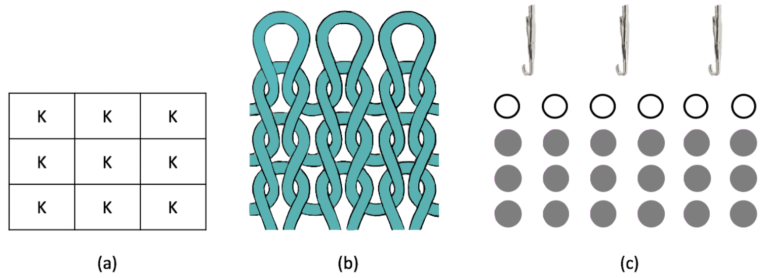
Figure 8: A 3x3 all-Knit stitch pattern: (a) Stitch pattern. (b) Resulting loops. (c) Corresponding Contact Neighborhoods.

Knit, Purl and Transfer Stitch
foo
j CN value before stitch execution j CN value after stitch execution j + 1 value (Knit $|$ Purl) j + 1 value (Transfer) null. PCN, [0,0] K$|$P, ACN, [0,0] null, PCN, [0,0] null, PCN, [${\Delta}i$,0] null, PCN, [${\Delta}i$,0] K$|$P, PCN, [${\Delta}i$,0] null, UACN$|$PCN, [0,0] null, UACN$|$PCN, [${\Delta}i$,0] null, UACN, [${\Delta}i$,0] K$|$P, UACN$|$ACN, [${\Delta}i$,0] null, UACN$|$PCN, [0,0] null, UACN$|$PCN, [${\Delta}i$,0] null, E, [0,-1] K$|$P, E, [0,-1] null, UACN$|$PCN, [0,0] null, UACN$|$PCN, [${\Delta}i$,0]

Table 1: Values set at data structure elements $(i,j)$ and $(i,j+1)$ when processing Knit, Purl and Transfer stitches.

4.3 Mappings

Since knitted textiles consist of more complicated stitches than just Knit and Purl, additional information is required to specify how the knitting process manipulates the CNs after they have been created from the loop formation process. For example, a Transfer stitch first produces a Knit or Purl stitch (thus creating ACNs at its legs and PCNs at its head), but then transfers, i.e. moves, the head of the stitch to a another nearby needle to its left or right. See Figure 4. These manipulations can be represented by mappings that capture the movement of the CNs and their state as they are transformed. The mappings that may be applied to CNs include two pieces of information,

1. an actualization value that specifies the state of the CN $(i,j)$ at its final location,

2. a vector that defines the CNs relative movement from its initial location in the CN $(i,j)$ grid.

These mappings specify an incremental, local transformation, i.e. the first immediate step in what could be a multi-step movement of the CN through the fabric. For example, a loop may be transferred to another needle, the loops at that needle could be tucked up to the next row of stitches, then another loop could be transferred onto the tucked destination. The incremental form of the mappings supports efficient, on-demand queries of the model, which is an unevaluated representation of the local processes that aggregate to form the final knitted textile.

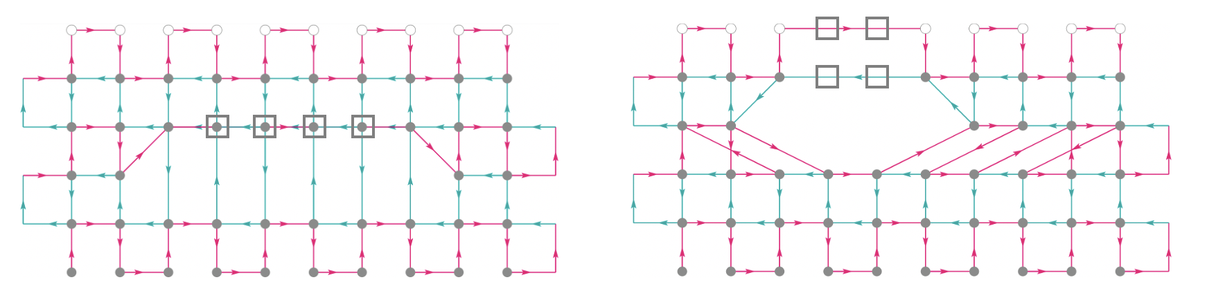
(a)                                   (b)

Figure 9: (a) Multiple consecutive Tuck stitches produce unanchored CNs (UACNs), displayed as squares. (b) Knit stitches executed on needles with no yarn loops also produce UACNs.

Tuck and Miss stitches apply different manipulations to the PCNs, moving them vertically, rather than horizontally. The Tuck stitch (Figure 5) shifts the PCNs $(i,j)$ and $(i+1,j)$ up to the next row of stitches and overlays them on PCNs $(i,j+1)$ and $(i+1,j+1)$. The Miss stitch (Figure 6) also shifts up PCNs to the next row, but by not hooking the $j^{\prime}th$ yarn the $j+1^{\prime}th$ CNs defined for this stitch (which are Empty) shift down one unit into the $j^{\prime}th$ row. Given the horizontal and vertical shifts that may occur, PCNs may end up at a different location and their actualization state might change or remain the same.

5 Data Structure

We have developed a data structure based on the process-oriented representation of Contact Neighborhoods (CNs) and associated mappings. The data structure can be populated with data derived from an $M\times N$ set of stitch instructions (e.g. Knit, Purl, Tuck, etc.) and produces a $2M\times(N+1)$ array of CNs. The $(i,j)$ index into the array effectively provides a unique ID for the CN created at this position in the fabric and also specifies a location in the $(i,j)$ grid for other CNs that move through the fabric. There is a direct relationship between the $(m,n)$ stitch instruction and the values stored at the four associated $(2m,n)$, $(2m+1,n)$, $(2m,n+1)$, $(2m+1,n+1)$ CNs. See Figure 7. At each $(i,j)$ element in the CN array three parameters are stored, which fully specify the CN that is created by the associated stitch instruction at that parameterized location in the knitted fabric, as well as information about the stitch itself.

The three parameters fall into two categories, location-based and CN-based. Location-based parameters, of which there is only one, store information that is specific to that $(i,j)$ location. CN-based parameters provide details about the CN that is created at location $(i,j)$, but which may be shifted to another location. The three parameters are: stitch type ST, actualization value AV and the movement vector $[{\Delta}i,{\Delta}j]$ MV. Each element in the data structure therefore takes the form of (ST, AV, MV).

5.1 Location-Based Parameter

The one location-based parameter (ST) gives information about the type of stitch to be formed when actualizing CNs that end up at location $(i,j)$. For example, if a Knit stitch is to be knitted at $(i,j)$, this would be specified with a ‘K’ in the corresponding element in the data structure. A ’P’ is stored for a Purl stitch. The stitch type parameter value determines how a CN at this location is actualized, whether the yarn is drawn through the loop(s) from back to front (Knit) or from front to back (Purl). In both of these cases firm contacts are formed between yarns via the twisting of the legs of a loop with the head of another loop, as seen in Figure 7(a). Note that since two CNs are created when a loop is formed, the stitch type for locations $(i,j)$ and $(i+1,j)$ will be the same.

5.2 CN-Based Parameters

The AV parameter indicates if a CN has been defined and, if so, it specifies the state of the CN as a result of the stitches executed during the knitting process. This parameter can take four values: PCN, ACN, UACN and E, as explained in Section 4.2.

The MV parameter $[{\Delta}i,{\Delta}j]$ indicates whether the CN is being shifted in either the horizontal or vertical direction. In the case of a Knit or Purl stitch, ${\Delta}i$ and ${\Delta}j$ are both 0, but when using other stitches, such as the Transfer stitch, their values would depend on the amount and direction of the movement needed for that specific stitch. A one needle movement to the left Transfer stitch (See Figure 4), has ${\Delta}i$ equal to -2 and ${\Delta}j$ equal to 0. Note that CNs are moved and not loops, which is why the CN is shifted two locations to the left rather than one. For a Tuck stitch, the vector is $[0,1]$, since the CN is shifted up to the next row. See Figure 5. The Miss stitch involves the movement of two sets of CNs. When Miss stitch data is written at location $(i,j)$, a CN may already exist at this location from the processing of a stitch instruction at $(i,j-1)$. The CN is shifted up to the next row using MV parameter value $[0,1]$. Instead of defining a CN at $(i,j+1)$ the yarn passes through and the CN that was supposed to be defined at $(i,j+1)$ is now shifted downward with MV $[0,-1]$. See Figure 6 for clarification.

Tuck and Miss Stitch
oo
j CN value before stitch execution j CN value after stitch execution j + 1 value (Tuck) j + 1 value (Miss) null. PCN, [0,0] null, PCN, [0,1] null, UACN, [0,0] null, E, [0,-1] null, PCN, [${\Delta}i$,0] null, PCN, [${\Delta}i$,1] null, UACN, [0,0] null, E, [0,-1] null, UACN, [${\Delta}i$,0] null, UACN, [${\Delta}i$,1] null, UACN, [0,0] null, E, [0,-1] null, E, [0,-1] null, E, [0,-1]* null, UACN, [0,0] null, E, [0,-1]

Table 2: Values set at data structure elements $(i,j)$ and $(i,j+1)$ when processing Tuck and Miss stitches. *Writing a Tuck and Miss stitch above a Miss stitch requires special processing away from the $j$ cell, as described below.

5.3 Populating the Data Structure

Given an $M\times N$ array of stitch instructions, a CN grid of size $(2M,N+1)$ is allocated. Each element in the grid is initialized as an Empty stitch, with the values (null, E, [null,null]), except the first row which we assume contain PCNs due to “cast-on” stitches that stabilize the bottom of the fabric. The stitch instructions are processed and CN values are assigned in a row-by-row, alternating left-right then right-left order, similar to the knitting process they represent. In general the data is written to these CNs in pairs, the lower pair, then the upper pair. The pre-condition state of the lower pair of CNs depends on the stitch instruction executed below them in the $n-1$ row. This state, along with the $(m,n)$ stitch instruction currently being executed, determine if and how the lower and upper pairs of CNs will be modified.

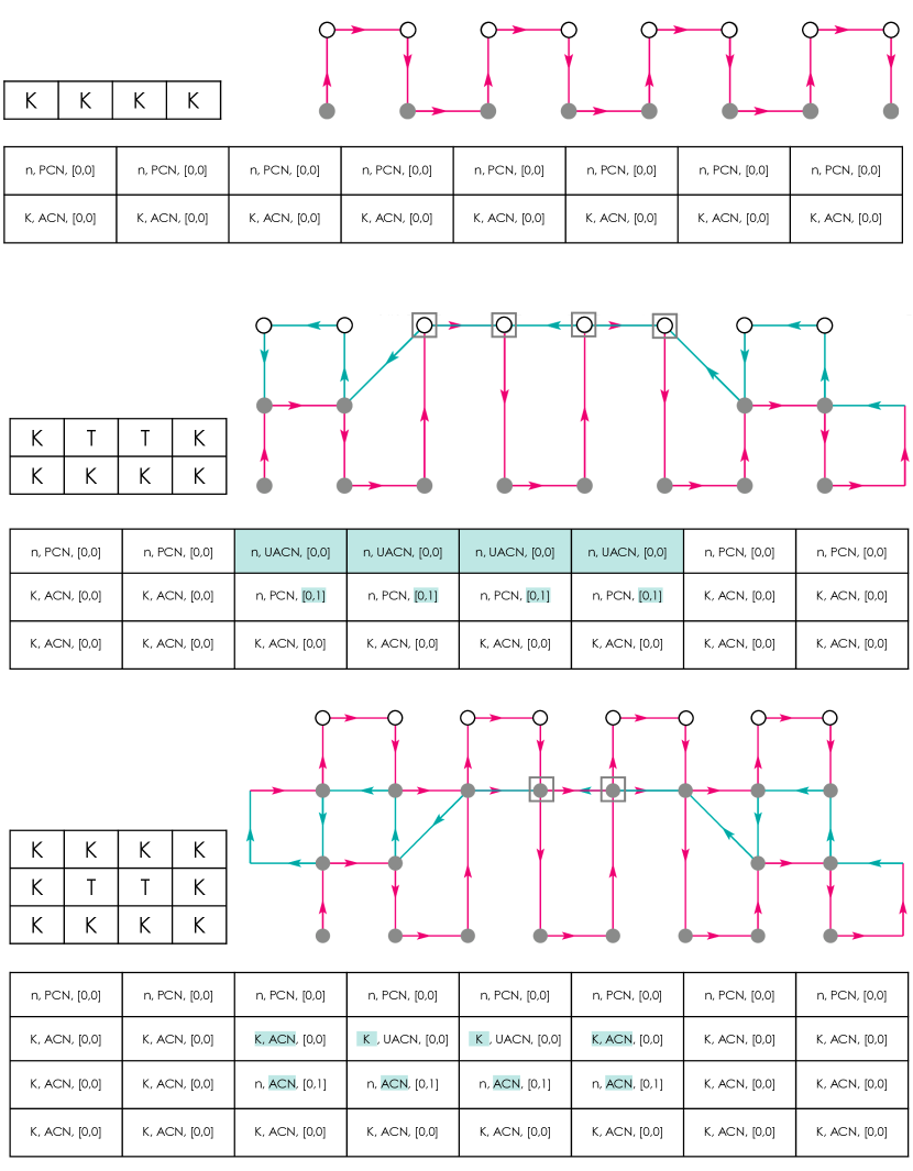
Figure 10: Determining if a UACN is anchored. (top) A row of Knit (K) stitches is written to the data structure. The resulting topology graph is on the upper right. (middle) Two Tuck (T) stitches are executed in the next row. This tucks up the CNs in the second row and creates four UACNs in the third row. The changes to the data structure are highlighted. (bottom) Another row of Knit stitches are written to the data structure. The outer UACNs are changed to ACNs, because they are connected to ACNs one row down and one column over. The tucked up loops are actualized (converted to ACNs) by the Knit stitches.

5.3.1 Knit, Purl and Transfer Stitches

Table 1 details how information related to Knit, Purl and Transfer stitch instructions is written into the CN data structure, depending on the pre-condition parameter values for the associated $(i,j)$ element. When modifying the lower CNs (the $j$ cells) two actions are consistently applied to the data structure values: A Knit or Purl stitch type is written in the ST parameter and the MV parameter is left unchanged. The AV parameter remains unchanged for a transferred PCN (a PCN with a non-zero ${\Delta}i$) and an Empty (E) CN state. AV is modified to ACN for a stationary PCN (a PCN where ${\Delta}i=0$). The AV parameter for transferred PCNs will be modified when actualized by a Knit, Purl or Transfer at their final location. A local operation is performed to determine if the UACN is truly unanchored. The UACN is changed to an ACN if the location down and over from the UACN holds an ACN, i.e. the UACN is actually anchored.

For the upper CN pair ($j+1$ cells), the ST parameter remains null. The AV parameter will be set to PCN if the $j$ cell is an ACN or if another CN is moved to the $j$ cell. Otherwise, no CN exists at the $j$ cell, which is one of the conditions for being unanchored; thus the $j+1$ cell’s AV parameter is set to UACN. The MV parameter has the value [0,0] for Knit and Purl stitches, since the loops of these stitches are not moved. See Figure 3. For the Transfer stitch the MV parameter is set to $[{\Delta}i,0]$, where ${\Delta}i$ can have the values $\pm 2,\pm 4,\pm 6$, depending on the direction and magnitude of the specified horizontal shift. See Figure 4.

Figure 10 details how UACNs are written and possibly modified while the CN data structure is being populated with Knit and Purl stitches. It consists of a stitch pattern, the associated topology graph and data structure elements. The top diagram shows the state of the data structure and the topology graph after four Knit stitches are processed. Given that the data structure is initialized with a row of PCNs, the Knit stitches actualize them and PCNs are written in the next row up. The Knit stitches in the second row produce the same result. The two Tuck stitches write ‘1’ to the ${\Delta}j$ component of the associated CNs and create UACNs above them.

Note at this point there are two sets of CNs at the four interior CN locations along the top of the structure. Four UACNs (designated with squares) from the teal yarn going right-to-left and four PCNs (designated with circles with white centers) from the two magenta loops that were tucked up one row. When the top row of Knit stitches are written to the data structure, the UACNs in the $j$ row are examined to determine if they might be anchored. The UACNs in the 3rd and 6th columns are anchored because they are connected to a local ACN one row down and one column over. The Knit stitch therefore actualizes them and their state is changed to ACN. The interior UACNs are not directly attached to ACNs in a lower row and therefore do not change their state. The PCNs tucked up from a lower row intertwine with the top yarn and are actualized to ACNs.

For more complex stitch patterns changing the state of an UACN to anchored and then actualized can require non-local information. For example, an UACN may be connected to an ACN in a lower yarn row, but several needle positions away, which can be seen in Figure 24. The lower ACN does anchor the upper CN. Determining this configuration and change of status requires tracing the yarn from the UACN to a possibly faraway CN, a non-local operation. Wanting the process of initially populating the data structure to be based on local information only, we decided to determine the final state of these UACNs at a later time, during the yarn tracing procedure.

5.3.2 Tuck and Miss Stitches

Table 2 details the parameter values that are written to the CN data structure for Tuck and Miss stitches. In the lower CNs ($j$ cells), the ${\Delta}j$ component of the MV parameter is set to 1, except for the Miss stitch precondition (${\Delta}j=-1$), which is left unchanged. See Figures 5 and 6. As signified by an asterisk* in the table, writing Tuck and Miss parameters values above a Miss stitch requires special processing away from the four cells that are normally affected by each stitch instruction. Since Tuck and Miss stitches effectively pull up the yarns held on the needle, a column of these stitches will pull the yarn up multiple rows. In order to capture this behavior, when writing a Tuck or Miss stitch above a Miss stitch, we move down the column looking for the first cell with a positive ${\Delta}j$ value. Once found, this cell’s ${\Delta}j$ value is then incremented by 1, indicating that associated CN has been pulled up one more row.

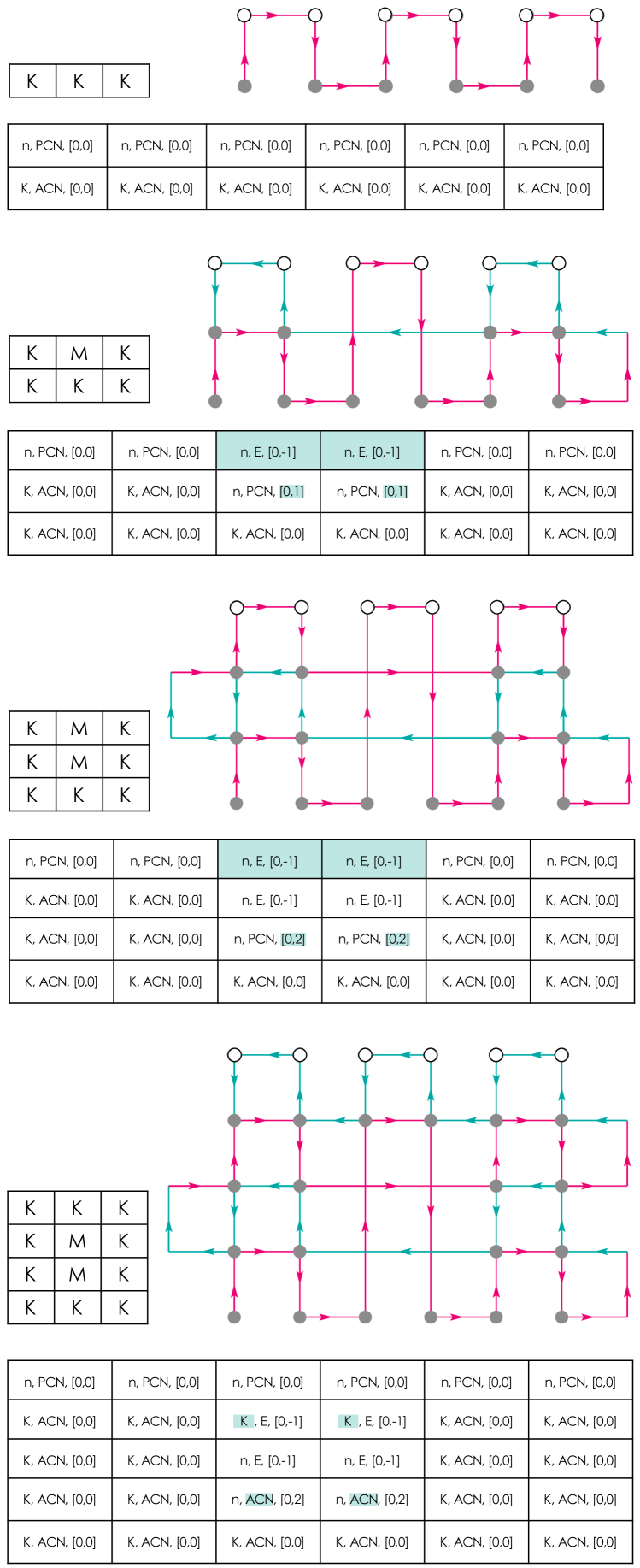
Figure 11: Updating ${\Delta}j$ of a Miss stitch. (top) A row of Knit (K) stitches is written to the data structure. The resulting topology graph is on the upper right. (middle top) A Miss stitch is executed in the middle of the pattern in the next row. This pulls up the held yarn and the traversing yarn crosses to the next stitch. An Empty stitch is written at $j+1$. (middle bottom) Another Miss stitch is executed above the previous one. The held loop is pulled up another row. Note that its ${\Delta}j$ has been incremented to 2. (bottom) A final row of Knit stitches actualizes the held loop.

The $j+1$ cells of all Tuck stitches are defined as unanchored, because a Tuck stitch does not make a yarn intertwining at location $(i,j)$. Thus the $j+1$ parameter values are set as (null, UACN, [0,0]). For the Miss stitch, no CNs are created at $j+1$, since the needle does not hook the traversing yarn. Thus the AV value is set to E (Empty) and the ${\Delta}j$ is set to -1, signifying that the yarn that should have passed through this location can be found in the next row down.

The special processing needed for Miss stitches is further explained in Figure 11. First, a row of Knit stitches are written to the data structure. The next row has a Miss stitch surrounded by Knit stitches. The Miss stitch changes the PCN’s ${\Delta}j$ to ‘1’ and writes “(null, E, [0,-1])” to the cell above. The next row has the same stitches. In this case, the cell values of the $j$ cell are left unchanged, and the CNs above the Miss stitch are also set to “(null, E, [0,-1])”. Note though that the ${\Delta}j$ values of the CNs that are pulled up another row have been set to ‘2’. The top row of Knit stitches actualize the two exterior sets of PCNs from the third row Knit stitches and the PCNs created by the Knit stitch at the center of the first row.

6 Topology Graph Algorithms

Given a stitch pattern, the TopoKnit data structure and associated algorithms can generate a topology graph of a knitted textile created with a single yarn. See Figures 15 to 24 for examples. The graph specifies how the yarn flows through the fabric and how points on the yarn contact other points on the yarn as it travels through the various stitches. The nodes in the graph, Contact Neighborhoods, represent yarn crossings/intertwinings and the edges of the graph represent the yarn segments that connect the yarn crossings. The nodes of the graph are located at discrete $(i,j)$ locations in a 2D grid, which are related to the $k^{\prime}th$ needle that created the associated stitch with the $l^{\prime}th$ row of the yarn. Zero, one or multiple nodes can be located at a single $(i,j)$ grid point.

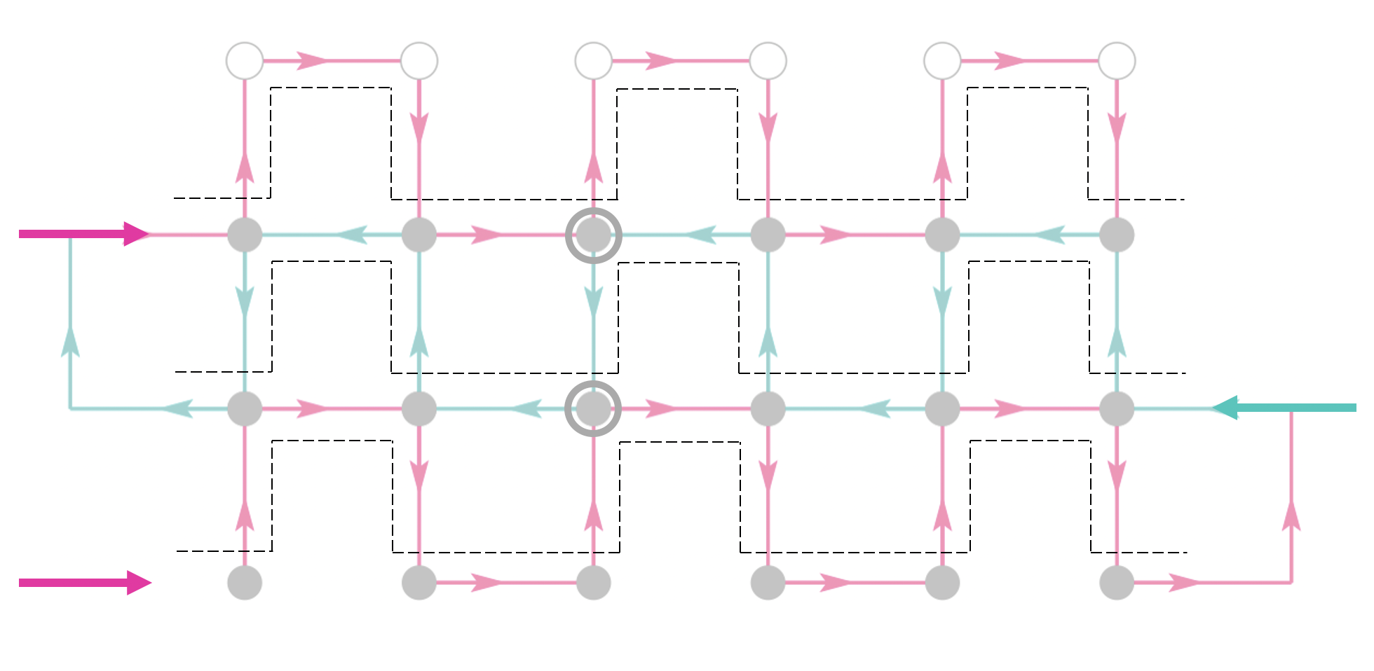
Figure 12: CNs processed in a square wave order for a 3x3 all-Knit pattern. The highlighted CNs are described Section 6.1.2.

6.1 Yarn Path Algorithms

Once populated with local stitch information, algorithms may be applied to the TopoKnit data structure to compute a variety of yarn-level topological data about the fabric produced by a given stitch pattern.

6.1.1 Follow-The-Yarn Algorithm

The main algorithm for extracting the yarn topology is called FOLLOW_THE_YARN and produces a sequential list of $(i,j)$ locations that the yarn passes through as it courses throughout the fabric. More specifically, each element in the yarn path list is a location that contains an ACN, i.e. this is a location where two or more yarns intertwine, with these ACN locations being sequentially ordered along the length of the yarn. An integer that identifies the current stitch row number, an important piece of information needed when determining the connectivity of an ACN, is also stored with the grid location.

The algorithm starts at location $(0,0)$ (bottom left) in the data structure and processes the CNs in a square-wave pattern as seen in Figure 12. The locations and associated CNs are processed along this path because it captures the order in which CNs are created and modified by the knitting process. The arrows on the sides of the figure indicate the direction that the yarn is carried for that row of stitches, first left-to-right (magenta arrow), then right-to-left (teal arrow), and so on. The square-wave pattern defines what we call leg nodes and head nodes. In this pattern a leg node CN is first processed (node $(i,j)$, assuming that the yarn direction is from left-to-right), followed by two head nodes ($(i,j+1)$ and $(i+1,j+1)$), and finally the other leg node CN ($(i+1,j)$). Note that with this pattern, two yarns flow into and out of each CN (except at the top and bottom rows, which can be stabilized with “cast-on” and “bind-off” stitches), once as a head node and once as a leg node. When representing an all-Knit pattern, all grid locations will be added to the yarn path, which makes its topology match the square wave (See Figure 12). Therefore the mappings for the other stitches effectively encode the local topological modifications that make the associated loops deviate from the default all-Knit structure.

Algorithm 1 $FOLLOW\_THE\_YARN(DS)$

$i,j,legNode,currentStitchRow\leftarrow 0,0,True,0$

$yarnPath\leftarrow[]$

while There are CNs to process do

    if $ADD\_TO\_LIST(i,j,legNode,yarnPath,DS)$ then

         if $legNode$ then

             $locInfo\leftarrow(i,j,currentStitchRow)$

         else$\triangleright$ Head node

             $locInfo\leftarrow\newline \mbox{\hskip 45.5244pt (FINAL\_LOCATION(i,j,DS),currentStitchRow)}$          

         $yarnPath.append(locInfo)$     

    $i,j,legNode,currentStitchRow\leftarrow\newline \mbox{\hskip 56.9055pt}NEXT\_CN(i,j,legNode,currentStitchRow)$ return yarnPath

As seen in Algorithm 1, the ADD_TO_LIST algorithm is invoked for each CN processed in the square wave order, and determines if the CN should be added to the yarn path. If the ADD_TO_LIST algorithm returns True, the legNode status of $(i,j)$ is checked. If it is a leg node, the $(i,j)$ grid location of the CN is added to the yarn path list. Since only head nodes are moved in the fabric during the knitting process, a leg node’s final location matches the location $(i,j)$ being processed. The FINAL_LOCATION algorithm is called to determine a head CN’s final location in the $(i,j)$ grid.

Once a CN is processed, the NEXT_CN algorithm computes the next $(i,j)$ location in the square wave, along with the leg node status of CN $(i,j)$, and updates the $currentStitchRow$ index if necessary.

Algorithm 2 $ADD\_TO\_LIST(i,j,legNode,yarnPath,DS)$

if $legNode$ then

    $numberOfACNs\leftarrow LENGTH(ACNS\_AT(i,j,DS))$

    if $numberOfACNs>0$ then $\triangleright$ Anchored CN is here

         return True

    else

         return False     

else$\triangleright$ Head node

    $actualizationValue\leftarrow DS[i][j].AV$

    if $actualizationValue==``E"$ then

         return False

    else if $actualizationValue==``UACN"$ then

         if $EVEN(i)==ODD(j)$ then $\triangleright$ Look backward

             $(m,n)\leftarrow Last\hskip 2.84526ptACN\hskip 2.84526ptin\hskip 2.84526ptyarn\hskip 2.84526ptpath$

         else$\triangleright$ Look forward

             $(m,n)\leftarrow Next$ $ACN$ $to$ $be$ $added$ $to$ $yarn$ $path$          

         $finalI,finalJ=FINAL\_LOCATION(i,j,DS)$

         if $n<finalJ$ then $\triangleright$ This CN is anchored

             $DS[i][j].AV\leftarrow``ACN"$ $\triangleright$ Update CN’s state

              return True

         else

              return False          

    else$\triangleright$ An ACN or PCN

         return True     

6.1.2 Add-To-List Algorithm

The two factors that determine whether a CN$(i,j)$ should be added to the yarn path list are the CN’s leg node status and its AV parameter. See Algorithm 2. Leg node CNs are processed first. The algorithm returns $True$ if there exists at least one actualized CN at location $(i,j)$. This signifies that the upper yarn was intertwined with another lower yarn at this location. Head nodes require examining the CN’s AV parameter. Empty CNs (E), which can be part of a Miss stitch or outside the boundary of the fabric, are not included in the yarn path list.

UACN head nodes require additional inspection to determine if they have been anchored by another CN further away along the yarn. This determination is performed by either looking back to the previous element in the yarn path or looking forward to find the next ACN to be inserted in the yarn path. The direction of the inspection is based on the structure of the square wave pattern and the parities of the $i$ and $j$ variables. The parity of $j$ indicates if the yarn is going from right to left (even) or left to right (odd) across the head of the loop, thus determining if the previous CN is at a lesser or greater $i$ value. For example, the first processed head node of a stitch is connected to a leg node “behind” it along the yarn. The second head node is connected to a leg node “in front of” it along the yarn. The parity of $i$ and $j$ values captures this first/second relationship, as seen in Figure 12. The lower circled CN has an $(i,j)$ value of $(2,1)$. When the parities are different the anchored check looks backwards. The upper circled CN has value $(2,2)$. When the parities are the same, the check looks forward along the yarn for a CN that might be at a lower $j$ value.

The final block of the AV check returns True, because all ACN and PCN head nodes are added to the yarn path list.

Algorithm 3 $FINAL\_LOCATION(i,j,DS)$

if $j==lastRow$ then $\triangleright$ CNs in the last row don’t move

   return i, j

else if $DS[i][j].{\Delta}i\hskip 2.84526pt!=0$ then$\triangleright$ Move CN horizontally

   return FINAL_LOC_RECURSIVE(i + DS[i][j].${\Delta}i$, j,DS)

else$\triangleright$ Move CN vertically

   return FINAL_LOC_RECURSIVE(i, j + DS[i][j].${\Delta}j$,DS)

Algorithm 4 $FINAL\_LOC\_RECURSIVE(i,j,DS)$

if $DS[i][j].ST==(K|P)$ then$\triangleright$ CN is actualized here

   return i, j

else$\triangleright$ Recursively accumulate vertical movements

   return FINAL_LOC_RECURSIVE(i, j + DS[i][j].${\Delta}j,DS$)

6.1.3 Final-Location Algorithm

Head node CNs can move within the $(i,j)$ grid, with their local movements encoded in the MV parameter. The FINAL_LOCATION function aggregates the movement information to determine the final location of the CN$(i,j)$ in the $(i,j)$ grid. Since a Transfer stitch actualizes two leg nodes (by creating a Knit or a Purl stitch) and then shifts its newly created head nodes left or right, a held loop (represented by two CNs) cannot be shifted vertically and then shifted horizontally; nor do horizontal CN shifts accumulate. Therefore, as seen in Algorithms 3 and 4, FINAL_LOCATION first applies horizontal movements, if any exist, before recursively calling FINAL_LOC_RECURSIVE to aggregate any possible vertical movements. See Figure 24. The final location is reached at a location where a Knit or Purl stitch is executed, which actualizes the CN moved to this location.

6.1.4 ACNS-At Algorithm

ACNS_AT (Algorithm 5) determines which ACNs are ultimately positioned at location $(i,j)$ in the CN grid, after the knitting process is complete. It computes in near constant time, since it executes the FINAL_LOCATION algorithm on a small finite set of CNs in a local neighborhood of $(i,j)$. It is only necessary to examine the local CNs because a loop of yarn can only be stretched a limited amount before it or the needle holding it breaks. Conventional knitting wisdom holds that a loop of yarn can only be stretched/moved away three needle positions horizontally or three yarn rows vertically. Additionally, since knitting is a sequential process, a loop at row $j+1$ cannot be shifted downwards to a previous, lower row. The physical properties of yarns therefore limit the distance over which they can be manipulated and leads to only requiring the examination of a $13\times 4$ neighborhood ($i-6\rightarrow i+6$, $j\rightarrow j-3$) around location $(i,j)$. FINAL_LOCATION is called for each CN$(i^{\prime},j^{\prime})$ in the neighborhood, and if this CN’s final location is $(i,j)$ and its AV state is $``ACN"$, it is added to the returned ACN list.

Algorithm 5 $ACNS\_AT(i,j,DS)$

$ACNList\leftarrow[]$

for all CN $(i^{\prime},j^{\prime})$ in the local 13 $\times$ 4 neighborhood do

    if $(FINAL\_LOCATION(i^{\prime},j^{\prime},DS)==(i,j))\hskip 2.84526pt\&\&$
                              $(DS[i^{\prime}][j^{\prime}].AV==``ACN")$ then

         $ACNList.append((i^{\prime},j^{\prime}))$     

return ACNList

Algorithm 6 $NEXT\_CN(i,j,legNode,currentStitchRow)$

if $BORDER\_CN(i,j,legNode)$ then

     return i, j+1, True, currentStitchRow + 1 $\triangleright$ Go up 1 row

else

    $nextI,nextJ=SQUARE\_WAVE(i,j,legNode)$

    $legNode=(nextJ==currentStitchRow)$

     return nextI, nextJ, legNode, currentStitchRow

Algorithm 7 $DRAW\_TOPOLOGY\_GRAPH()$

$CNList=FOLLOW\_THE\_YARN()$

$n\leftarrow len(CNList)$

$\triangleright$ Draw the first disk                                                                      

if $DS[0][0].ST==K$ then

    $DRAWDISK(0,0,gray)$

else$\triangleright$ Stitch type is P

    $DRAWDISK(0,0,green)$ $\triangleright$ Loop through the yarn list CNs                                              

for $CNIndex\leftarrow 0\hskip 2.84526ptto\hskip 2.84526ptn-2$ do

    $currentI,currentJ,currentStitchRow\leftarrow\newline \mbox{\hskip 147.95433ptCNList[CNIndex]}$

    $nextI,nextJ,nextYarnRow\leftarrow CNList[CNIndex+1]$ $\triangleright$ Draw graph node                                                                       if $DS[nextI][nextJ].AV==``PCN"$ then $\triangleright$ Last CN row          $DRAWDISK(nextI,nextJ,white)$     else$\triangleright$ Draw ACN disk          if $DS[nextI][nextJ].ST==K$ then              $DRAWDISK(nextI,nextJ,gray)$          else$\triangleright$ Stitch type is P              $DRAWDISK(nextI,nextJ,green)$              $\triangleright$ Draw graph edge                                                                   $legNode=(currentJ==currentStitchRow)$     if $ODD(currentStitchRow)$ then          $yarnColor\leftarrow teal$     else          $yarnColor\leftarrow magenta$          if $BORDER\_CN(currentI,currentJ,legNode)$ then          $DRAWLOOP(currentI,currentJ,nextI,nextJ,$
                                                           $yarnColor)$     else          $DRAWARROW(currentI,currentJ,nextI,nextJ,$
                                                           $yarnColor)$          if $currentJ==nextJ$ then $\triangleright$ Checking for UACNs          for $testedI\leftarrow currentI\hskip 2.84526ptto\hskip 2.84526ptnextI$ do              if $DS[testedI][currentJ].AV==``UACN"$ then                  $DRAWSQUARESTROKE(testedI,$
                                                       $currentJ,gray)$                           

6.1.5 Next-CN Algorithm

After each CN is processed in the FOLLOW_THE_YARN algorithm, the next CN in the square wave is generated by the NEXT_CN algorithm (Algorithm 6). This algorithm usually invokes the SQUARE_WAVE algorithm, which in turn uses logic based on the values of $i$, $j$ and $legNode$ to compute $nextI$ and $nextJ$. This logic was determined by studying the path the yarn follows in an all-Knit pattern.

The new location is a leg node if $nextJ$ equals $currentStitchRow$. If $(i,j)$ is on the border of the stitch pattern, the $j$ index, which identifies the row of the CN, and $currentStitchRow$ are incremented and the leg node status is set to True. This encodes that a yarn loops up to the next row to a leg node position when it reaches the end of a row of stitches.

6.2 Drawing the Topology Graph

The topology graph information extracted from the algorithms described in Section 6.1 can be visualized using Algorithm 7. This algorithm iterates through the list of locations returned by Algorithm 1 and invokes different drawing routines to draw the nodes and edges of the graph. To more easily identify the path of the yarn through the graph, two different line colors are used to represent the yarn. When knitting an even row, when the yarn flows from left to right, the yarn/edge color is magenta. When knitting an odd row, when the yarn flows from right to left, the yarn/edge color is teal. The graph contains different types of CNs, and icons with different shapes and colors are used to distinguish them from each other. Colored disks are used for ACNs and PCNs, gray for knit ACNs, green for purl ACNs and white for PCNs. UACNs that lie along horizontal yarns are detected by Algorithm 7 and gray squares are drawn to represent them at their grid locations. Currently, we only display a single disk at any location $(i,j)$, even if more than one CN ends up at the location. However, the total number of arrows going in and out of a node can provide information about the number of CNs at a given location.

Algorithm 7 loops through the locations of the ACNs, generated by Algorithm 1, that are sequentially ordered along the yarn that courses through the fabric defined by the given stitch pattern. At each iteration of the loop, the algorithm draws an arrow from the current CN location to the next CN location in the list. The arrow represents the yarn that connects the two CNs and the direction of the arrow corresponds to the direction of the yarn during the knitting process. The arrow color is determined by the yarnColor variable, which is based on the parity (and direction) of the current yarn row. When the current list element is on the border of the fabric, three arrows are drawn which loop the yarn around to the next row being visualized. The first two arrows have the same color as the yarnColor value and the last arrow has the other color, to show that a new row is beginning.

It is important to note when the current location and next location in the yarn list have the same $j$ value there might be UACNs existing between them. The algorithm checks all CNs between the current CN location and the next CN location and draws squares for CNs with actualization values equal to UACN. A slightly modified version of Algorithm 7 can be used to generate row-by-row topological graphs for a given stitch pattern as seen in Figure 16. This allows us to view the state of the topology graph as the fabric is being constructed and helps to highlight how the CN actualization values change during the knitting process.

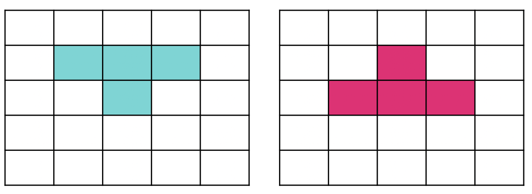
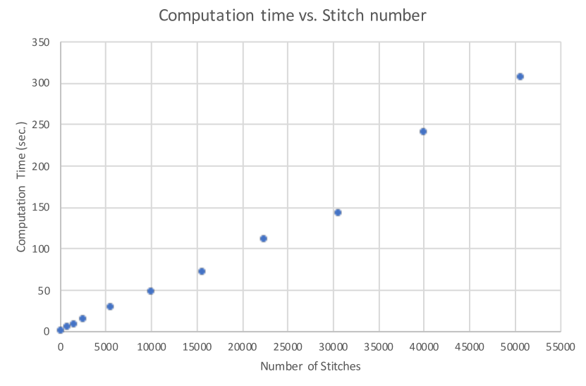
Figure 13: Teal and magenta stitch pattern templates.

Figure 14: Plot of timing values from Table 3 that demonstrates the linear time complexity, as a function of the number of stitches, of TopoKnit’s evaluation algorithms.

Pattern Size	# Stitches	Time (sec.)
10 $\times$ 10	100	0.443
30 $\times$ 30	900	5.51
40 $\times$ 40	1,600	8.81
50 $\times$ 50	2,500	14.8
75 $\times$ 75	5,625	29.0
100 $\times$ 100	10,000	48.0
125 $\times$ 125	15,625	71.6
150 $\times$ 150	22,500	111
175 $\times$ 175	30,625	142
200 $\times$ 200	40,000	240
225 $\times$ 225	50,625	307

Table 3: Computation times (in seconds) needed to generate and evaluate repeating blocks of the stitch pattern in Figure 15. The first column contains the dimensions of the stitch pattern. The second column contains the total number of stitches in the swatch and the last column contains the time needed for the computation.

7 Results

The TopoKnit representation and associated algorithms were tested with 100 $5\times 5$ stitch patterns in order to assess the robustness, accuracy and effectiveness of our approach to evaluating the topology of knitted fabrics. The test patterns were generated by randomly selecting stitches for each cell in the teal and magenta areas in the grids presented in Figure 14. The set of selected stitches included Knit, Transfer right, Transfer left, Tuck and Miss stitches. All of the white cells were defined as Knit stitches. TopoKnit generated 100 correct topology graphs from these 100 stitch patterns. The correctness of our results was confirmed by comparisons with graphical outputs from the Shima Seiki SDS-One APEX3 KnitDesign system.

Figures 15, 16 and 17 use the magenta template and Figures 19 and 19 use the teal template and produce complex yarn topologies from relatively simple combinations of Knit, Transfer, Tuck and Miss stitches. Additionally a number of other patterns were tested that included empty stitches around the pattern border to produce increases and decreases in the fabric, as well as a set of (light green) 3-level patterns, such as the ones in Figures 24, 24 and 24. These additional tests also produced correct topology graphs of the resulting fabrics.

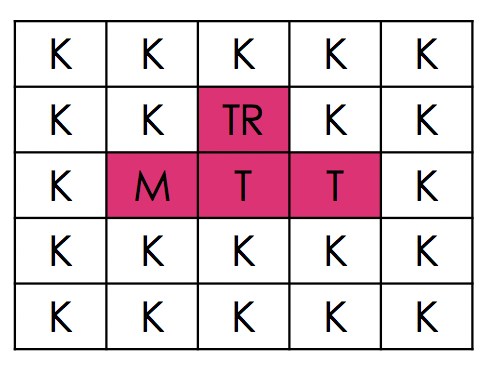
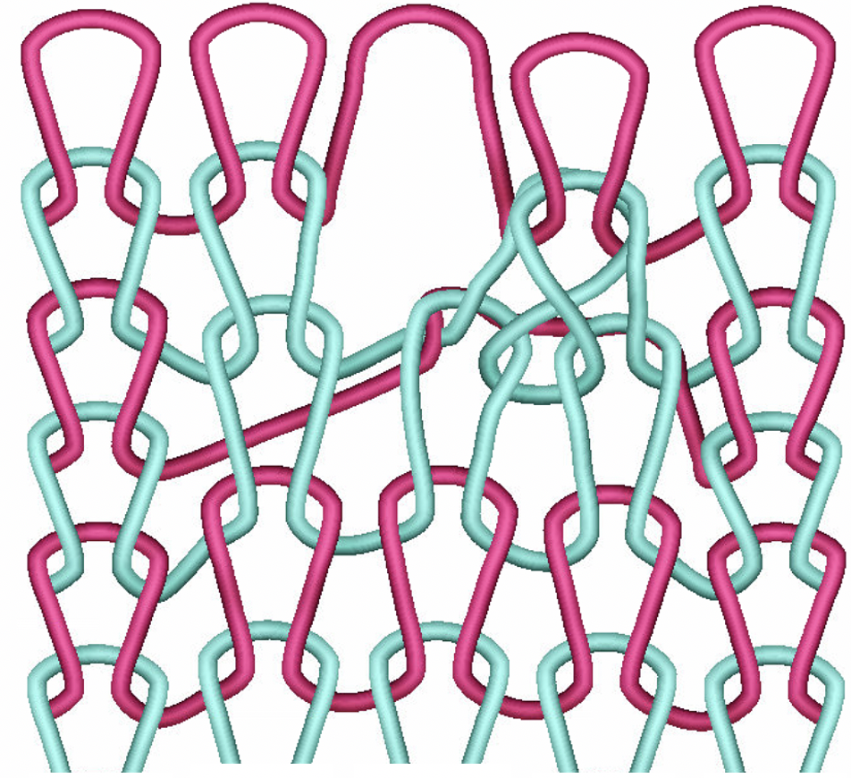
(a)              (b)                                                                    (c)

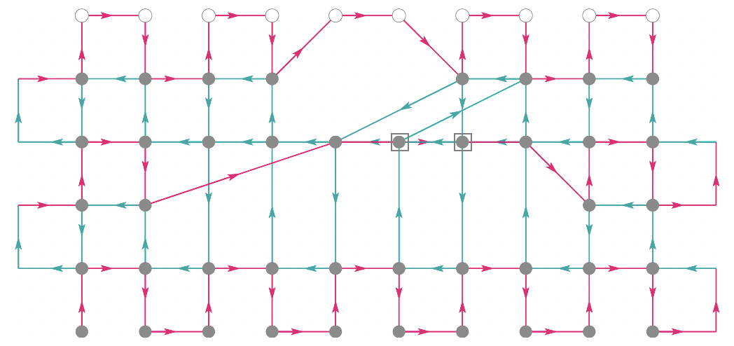
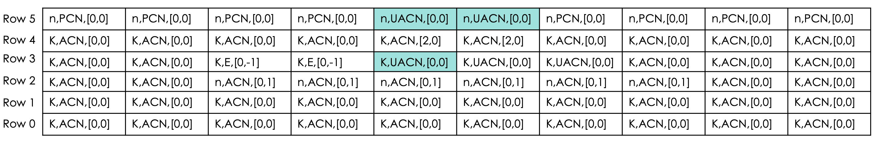
                                                                          (d)


                                                                          (e)

Figure 15: Stitch pattern with a combination of Knit, Transfer, Miss and Tuck stitches: (a) Stitch instructions. (b) Simulation of stitch pattern. (c) Topology graph. (d) Corresponding data structure before evaluation. (e) Modified entries (highlighted in teal) in data structure after evaluation.

Figure 15 presents an example stitch pattern that includes Knit, Transfer, Tuck and Miss stitches. The (a) figure is the stitch pattern for this swatch. The (b) figure is graphical output from the Shima Seiki SDS-One APEX3 KnitDesign system for the stitch pattern. . The (c) figure is the topology graph of the resulting fabric automatically generated by our algorithms.

Figure 15(d) presents the initial populated data structure and 15(e) presents the state of the data structure after the updates executed in the FOLLOW_THE_YARN algorithm. Note that UACNs have been updated to PCNs in the top row and an ACN in the third row by Algorithm 1. Cells $(4,4)$ and $(5,4)$ in the data structure have a non-zero ${\Delta}i$, which means that these two CNs have been shifted to the right as can be visually seen in the topology graph. Two interesting locations in the diagram are locations $(5,3)$ and $(6,3)$, which in addition to the ACNs shown with grey circles have at least one UACN represented by the outlined square. The magenta and teal directed edges are the yarns that connect the CNs, with the arrows showing the direction the yarn was carried during the knitting process. At least two yarns flow into and out of each ACN and form the yarn contact at that location.

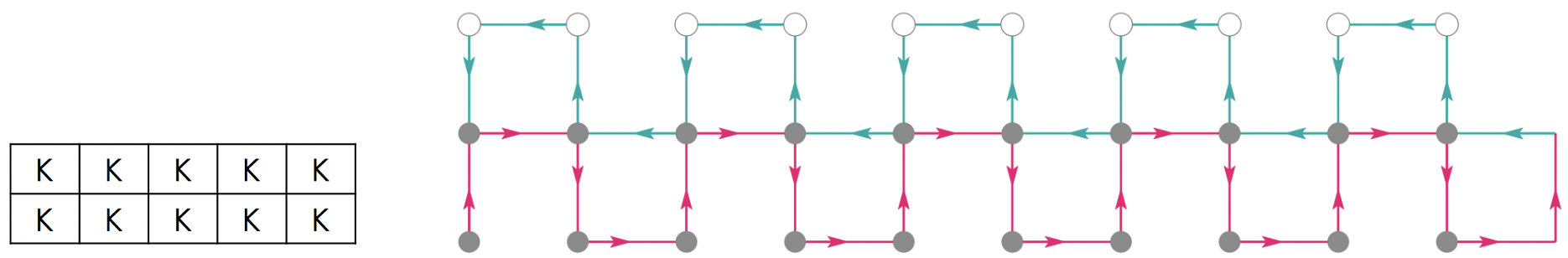
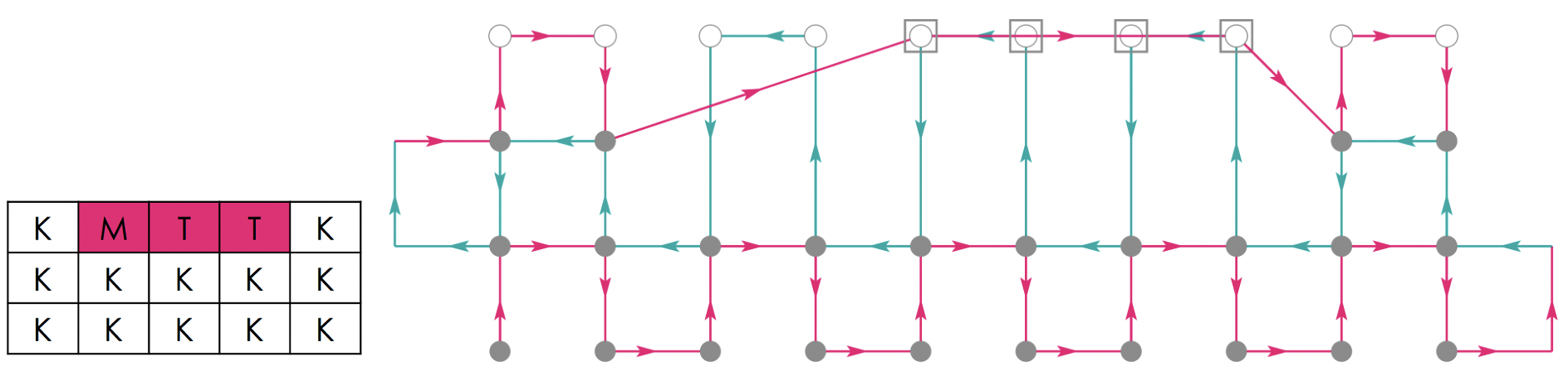
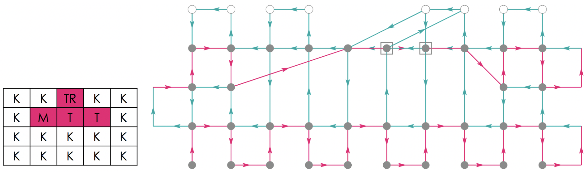
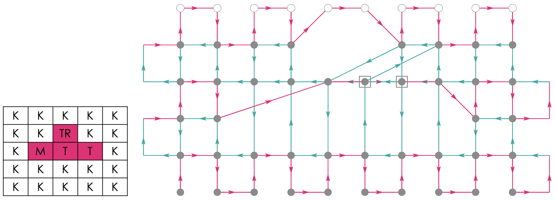
Figure 16: The topology graph produced from a stitch pattern that includes Knit, Transfer, Miss and Tuck stitches. The descending diagrams present the topological state of the fabric as it is knitted row by row.

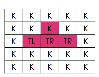
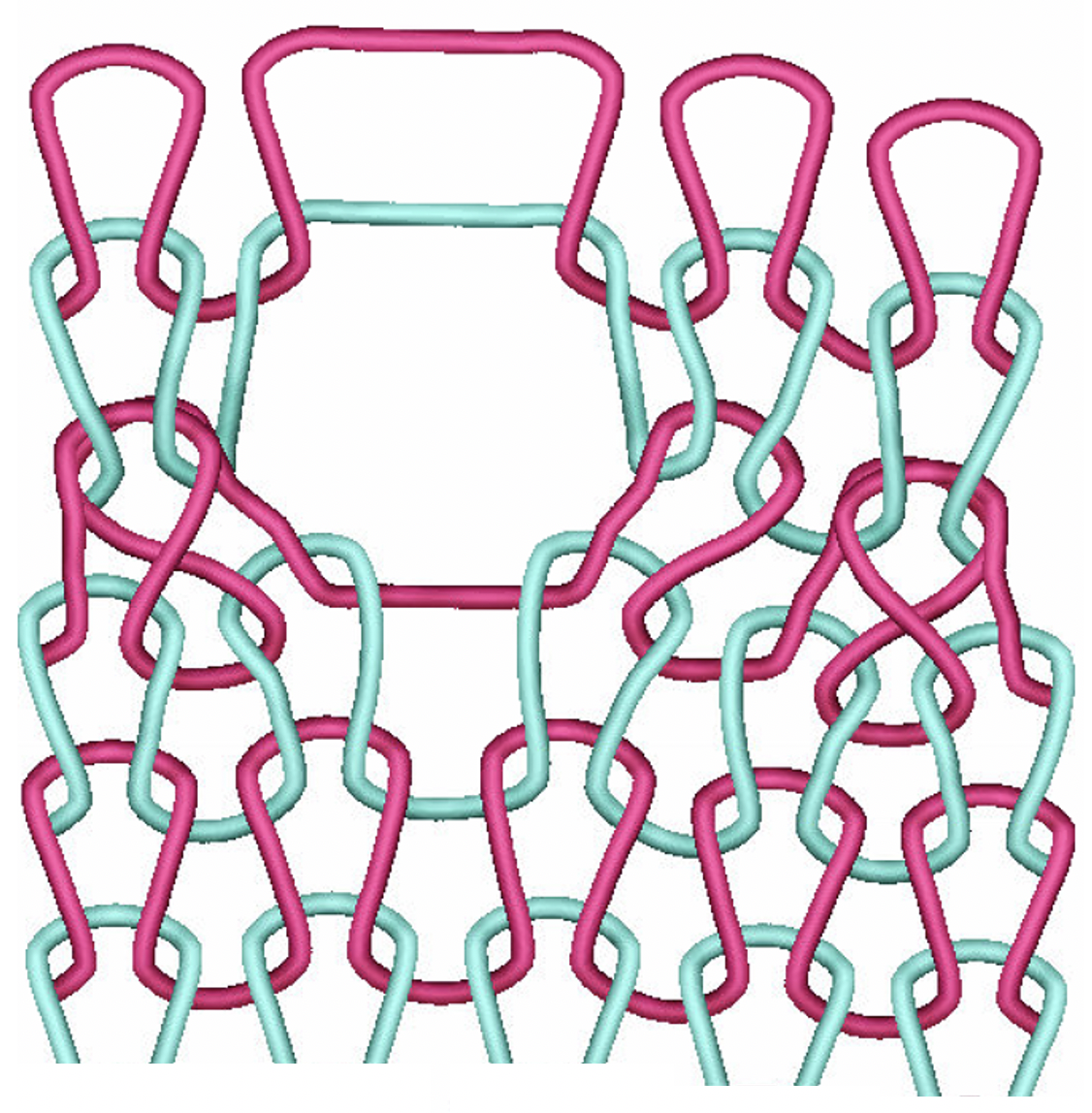
(a)              (b)                                                                    (c)

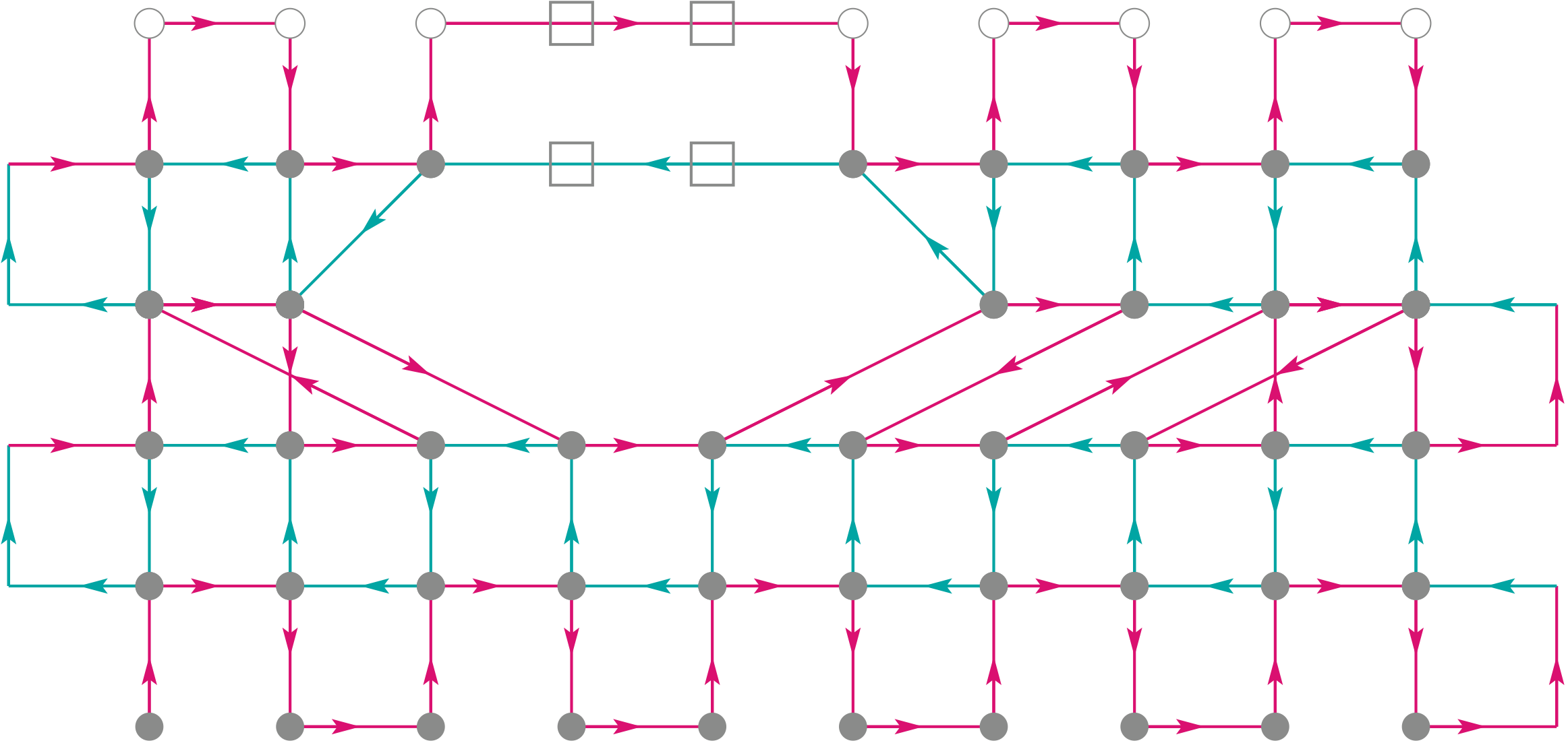
Figure 17: Stitch pattern with a combination of Knit and Transfer stitches: (a) Stitch instructions. (b) Simulation of the pattern. (c) Topology graph. The pattern creates a “hole” in the fabric and an ascending “ladder” of unanchored CNs.

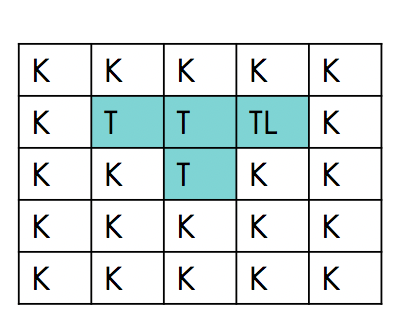
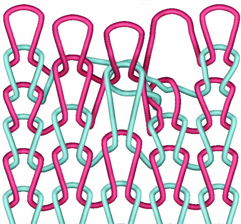
(a)              (b)                                                                    (c)

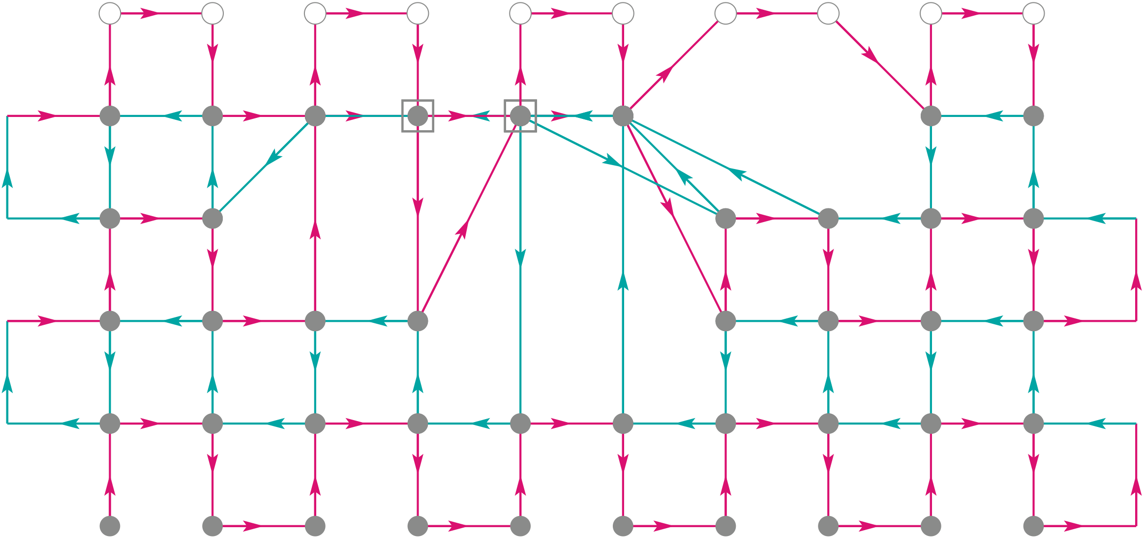
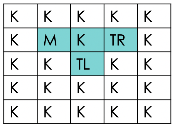
Figure 18: Stitch pattern with a combination of Knit, Tuck and Transfer stitches: (a) Stitch instructions. (b) Simulation of the pattern. (c) Topology graph.

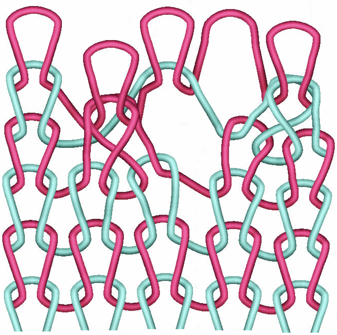
(a)              (b)                                                                    (c)

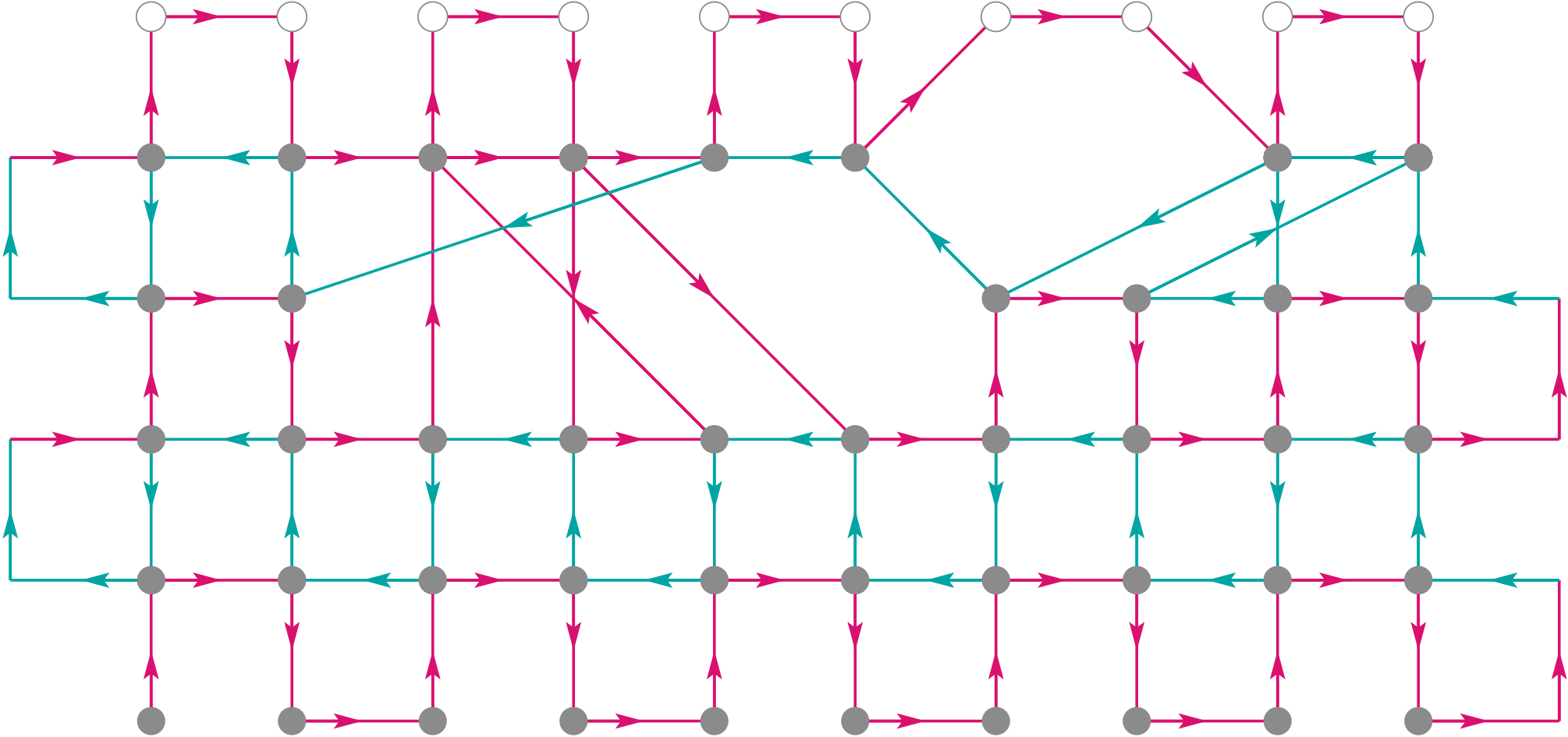
Figure 19: Stitch pattern with a combination of Knit, Miss and Transfer stitches: (a) Stitch instructions. (b) Simulation of the pattern. (c) Topology graph.

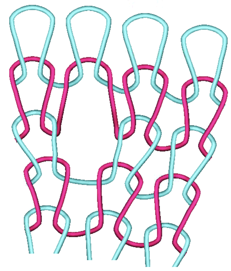
(a)              (b)                                                                    (c)

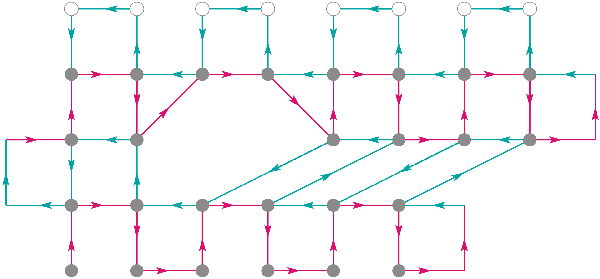
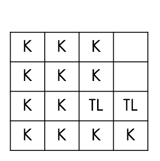
Figure 20: An increase of the fabric using Transfer and Empty stitches: (a) Stitch instructions. (b) Simulation of the pattern. (c) Topology graph.

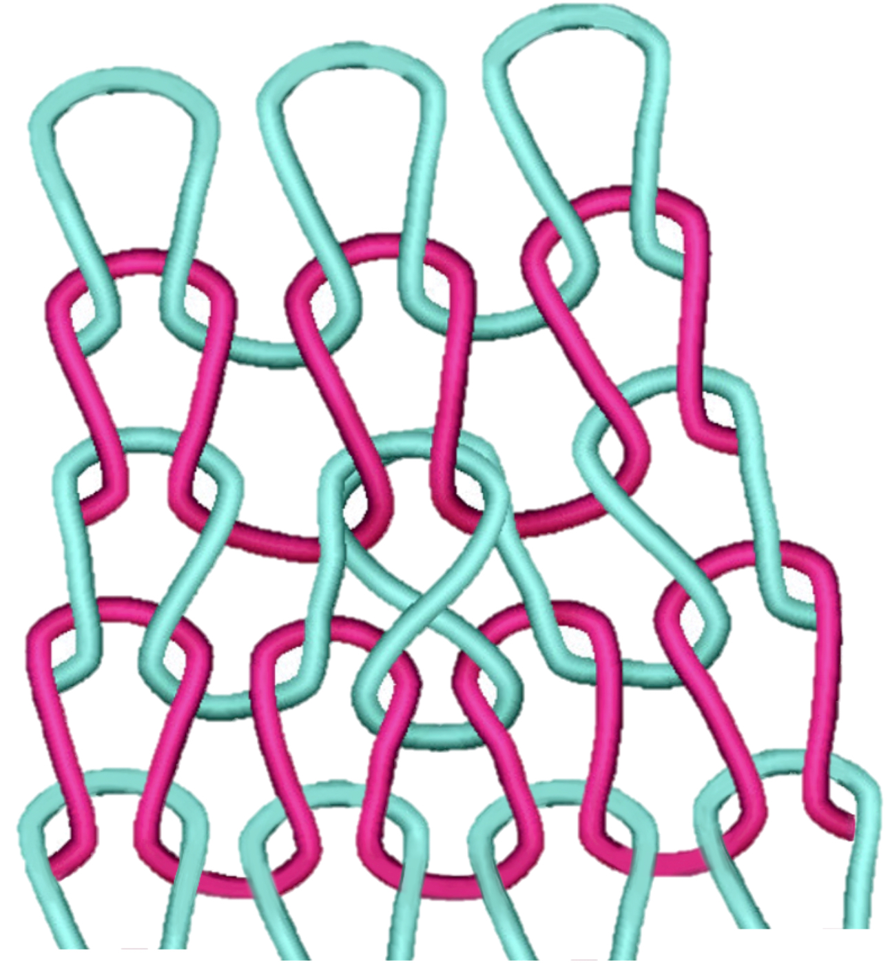
(a)              (b)                                                                    (c)

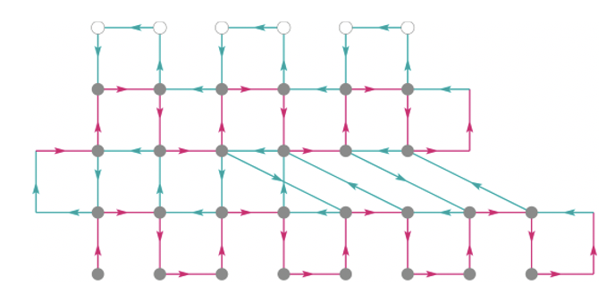
Figure 21: A decrease of the fabric using Transfer and Empty stitches: (a) Stitch instructions. (b) Simulation of the pattern. (c) Topology graph.

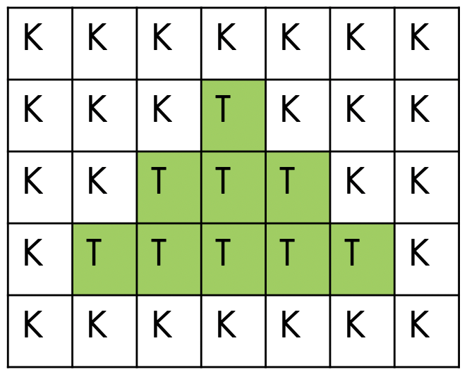
(a)              (b)                                                                    (c)

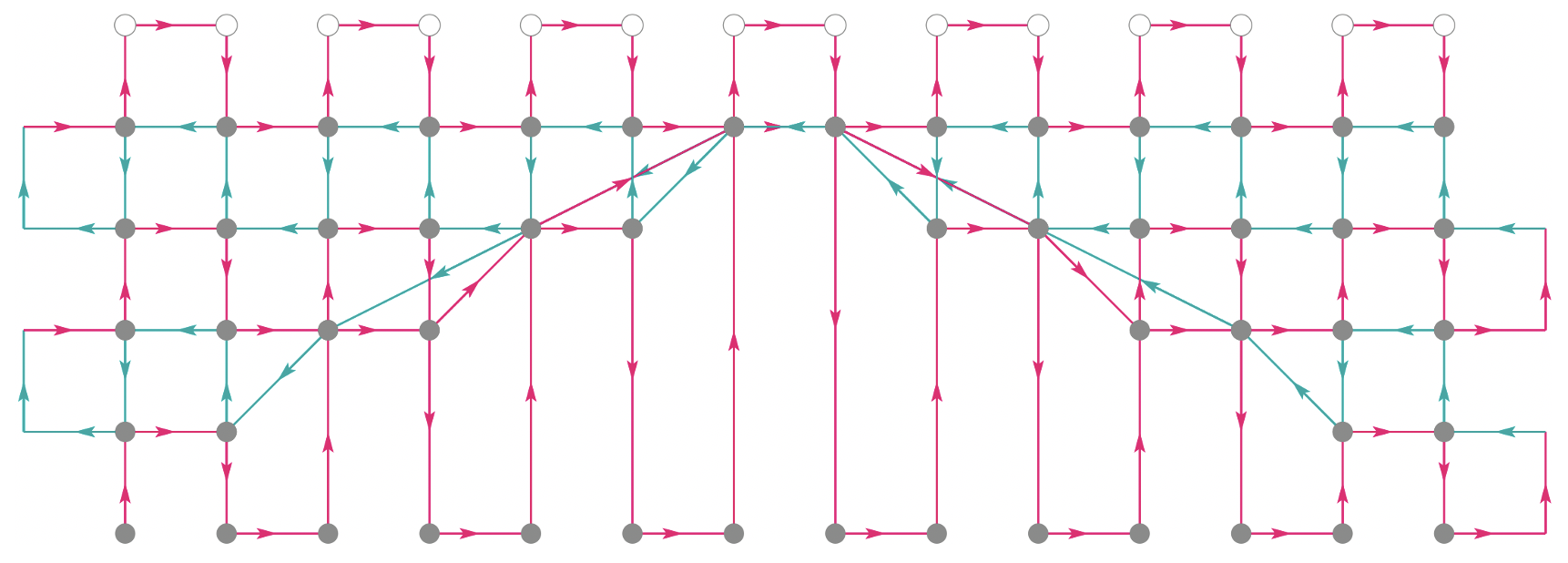
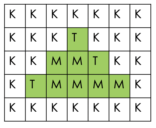
Figure 22: Pattern with a 3-level combination of Knit and Tuck stitches: (a) Stitch instructions. (b) Pattern simulation. (c) Topology graph.

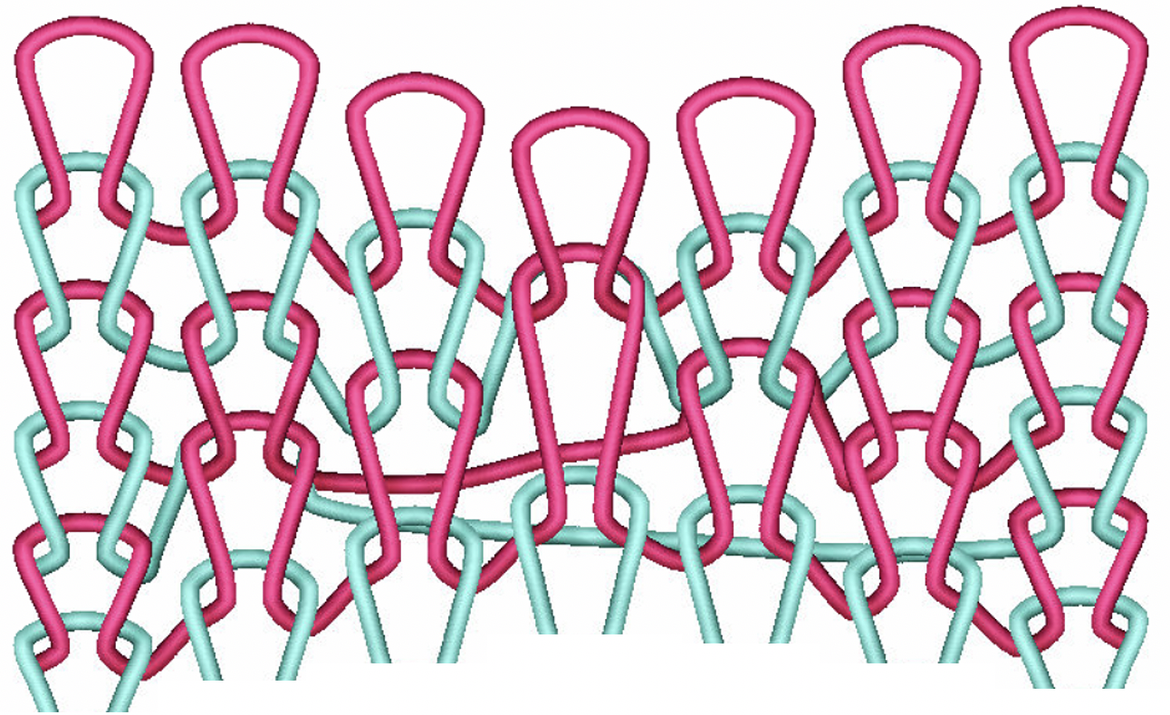
(a)              (b)                                                                    (c)

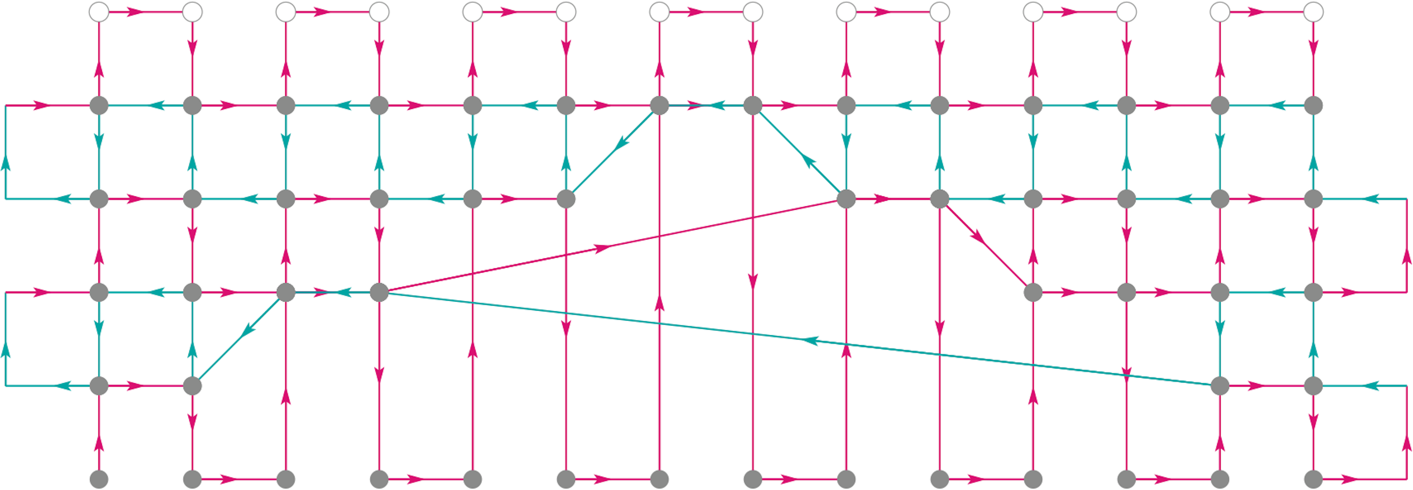
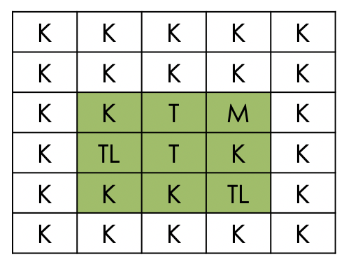
Figure 23: Pattern with a 3-level combination of Knit, Miss and Tuck stitches: (a) Stitch instructions. (b) Pattern simulation. (c) Topology graph.

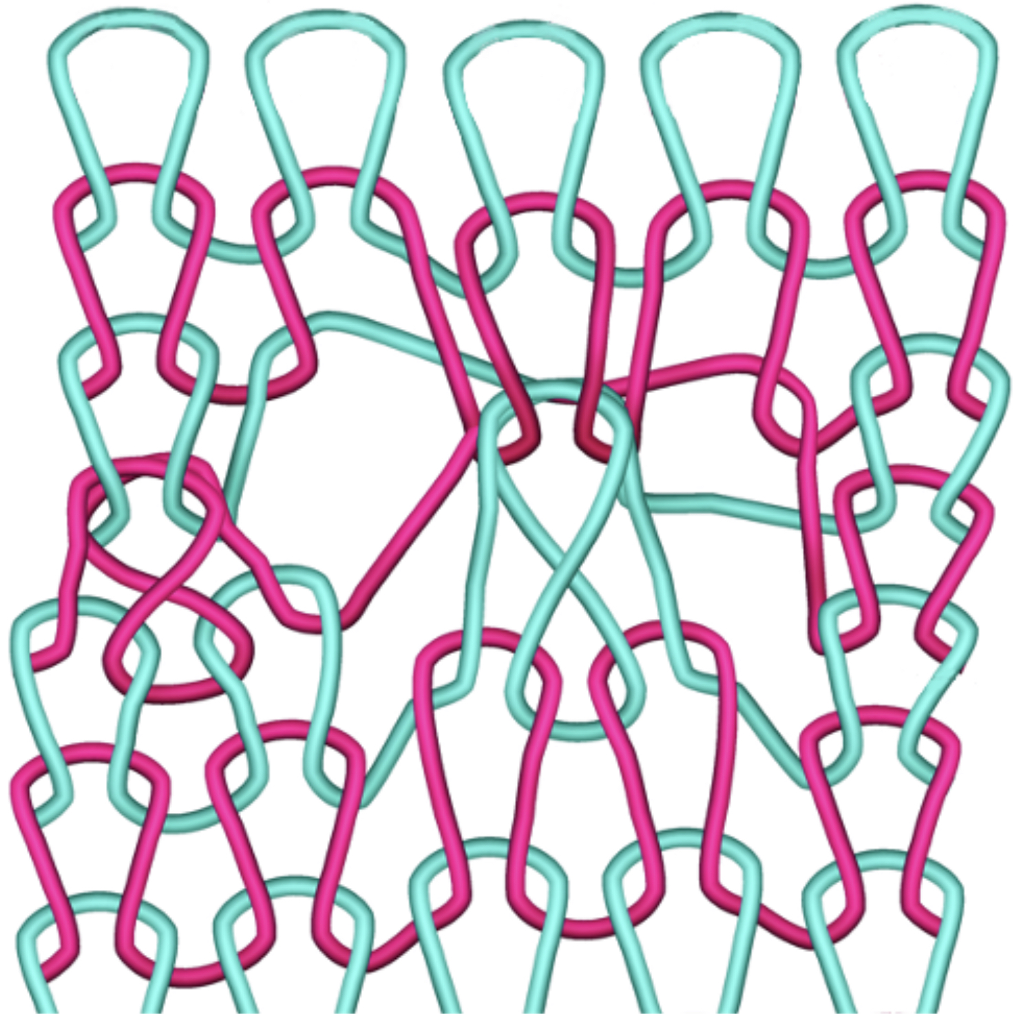
(a)              (b)                                                                    (c)

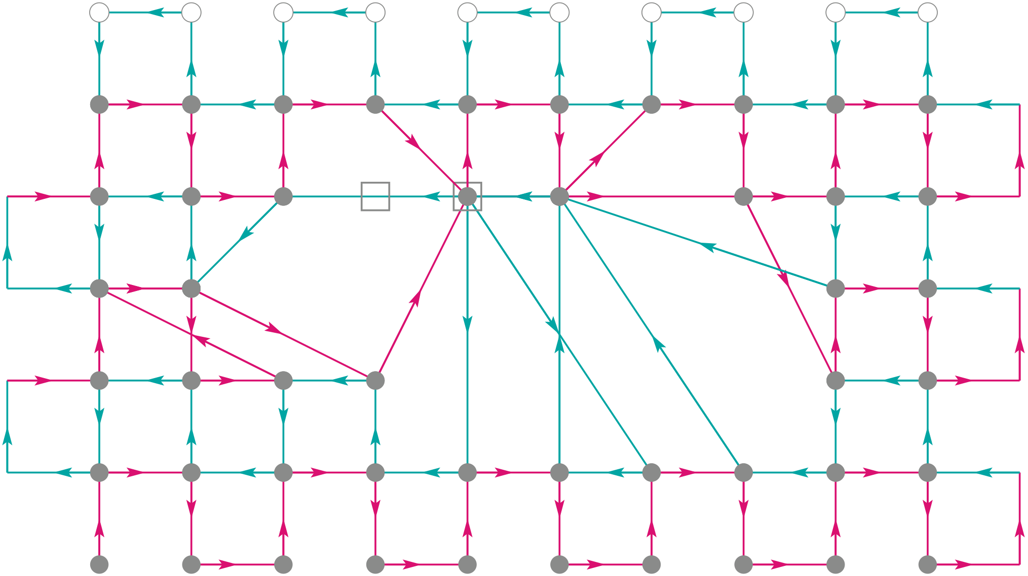
Figure 24: Pattern with a combination of Knit, Transfer, Tuck and Miss stitches: (a) Stitch instructions. (b) Pattern simulation. (c) Topology graph.

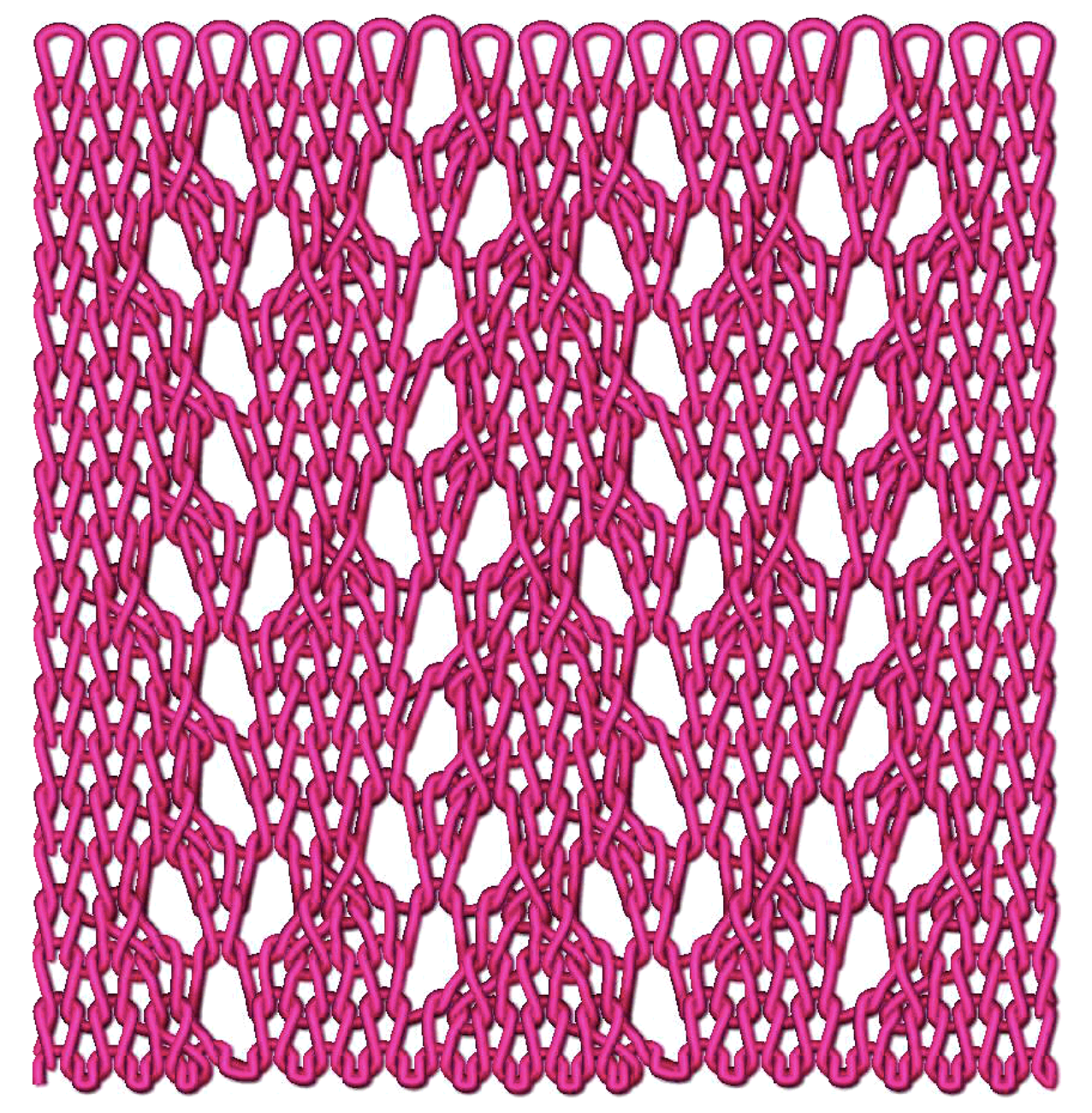
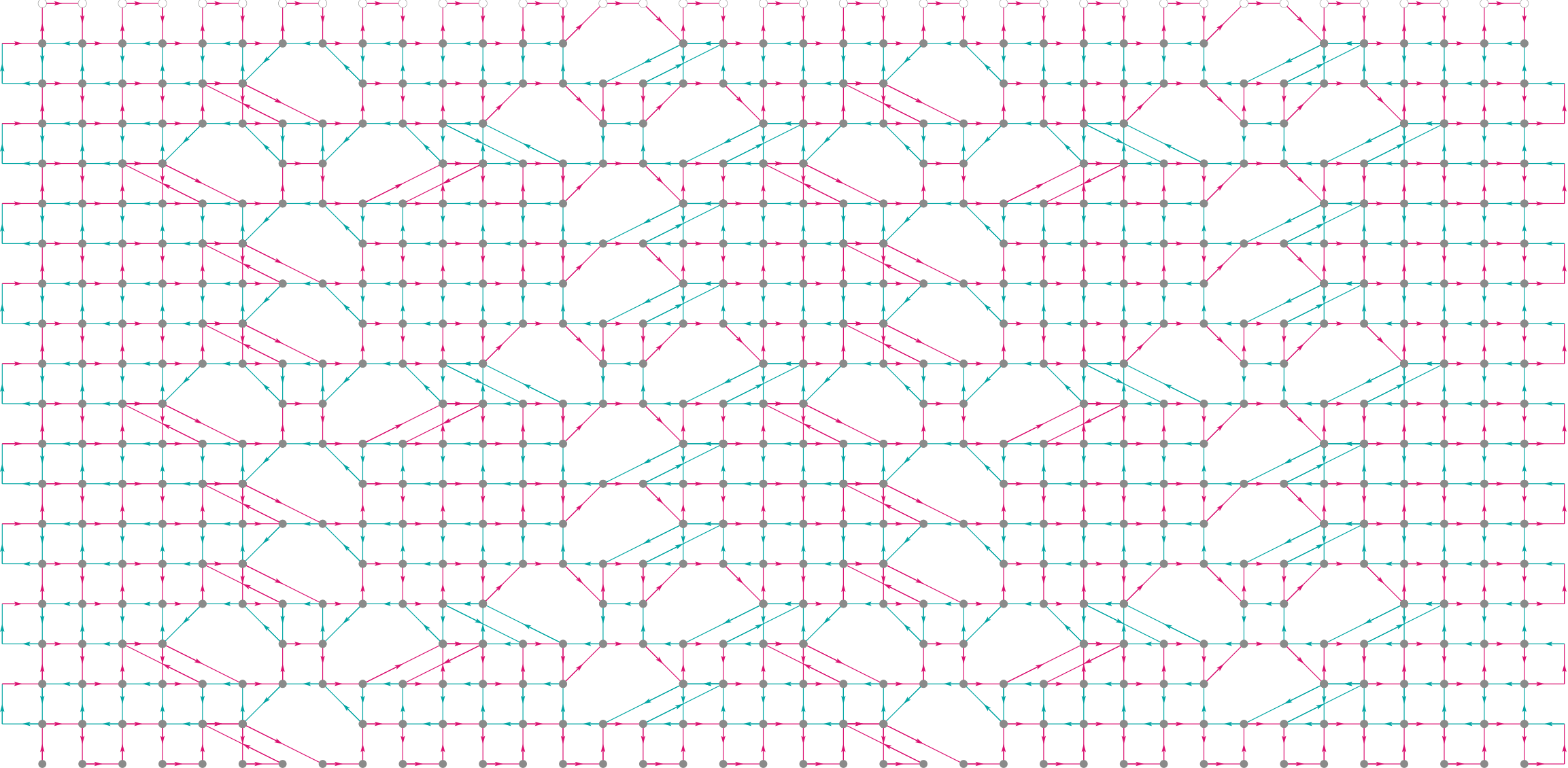
(a)                                                                          (b)

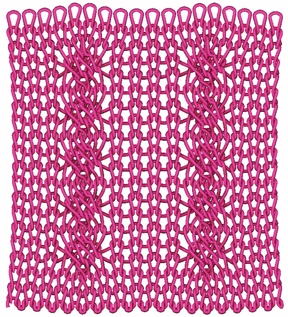
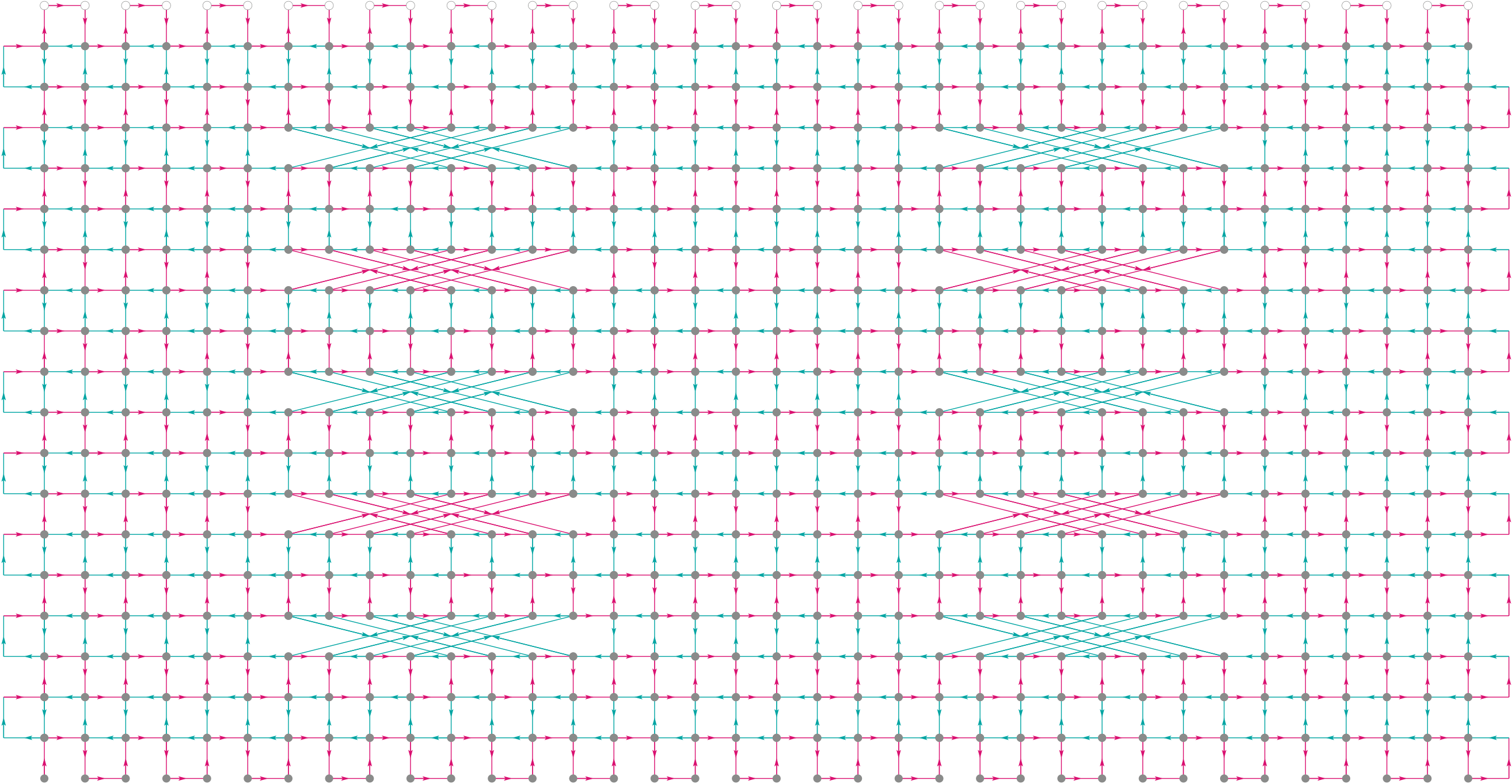
(c)                                                                          (d)

Figure 25: Samples of larger stitch patterns and their corresponding topology graphs: (a) Simulation of a lace pattern. (b) Topology graph of the lace pattern. (c) Simulation for a cable pattern. (d) Topology graph of the cable pattern.

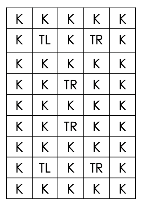
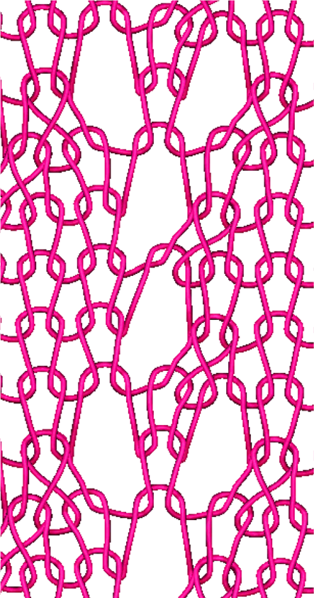
(a)              (b)                                                                    (c)

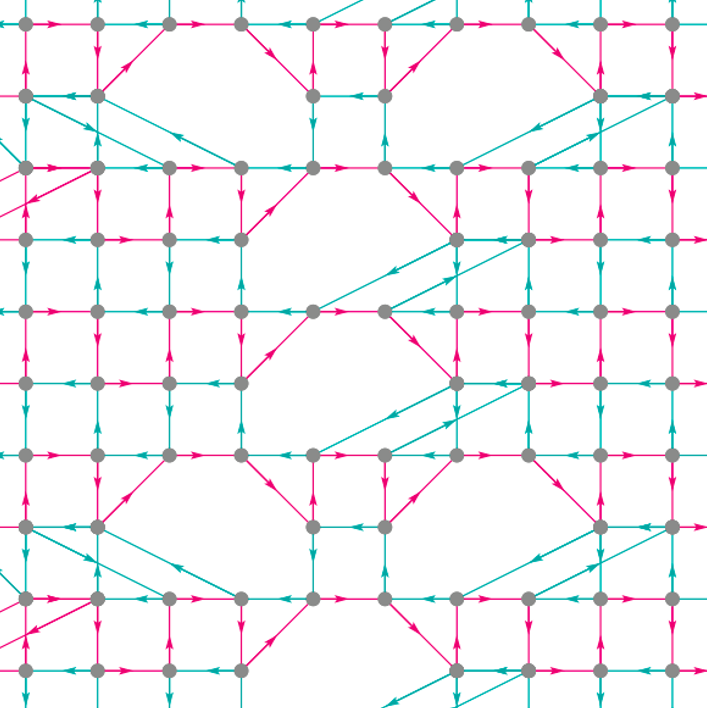
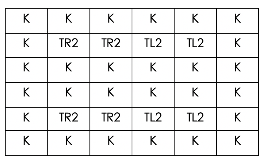
Figure 26: A closer view of the lace pattern: (a) Stitch instructions. (b) Simulation of the pattern. (c) Topology graph.

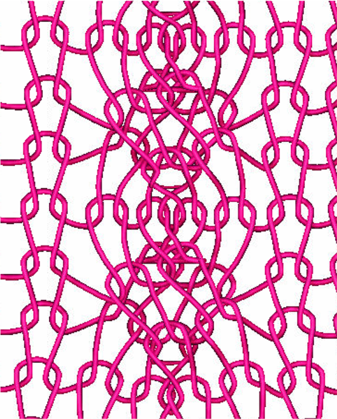
(a)              (b)                                                                    (c)

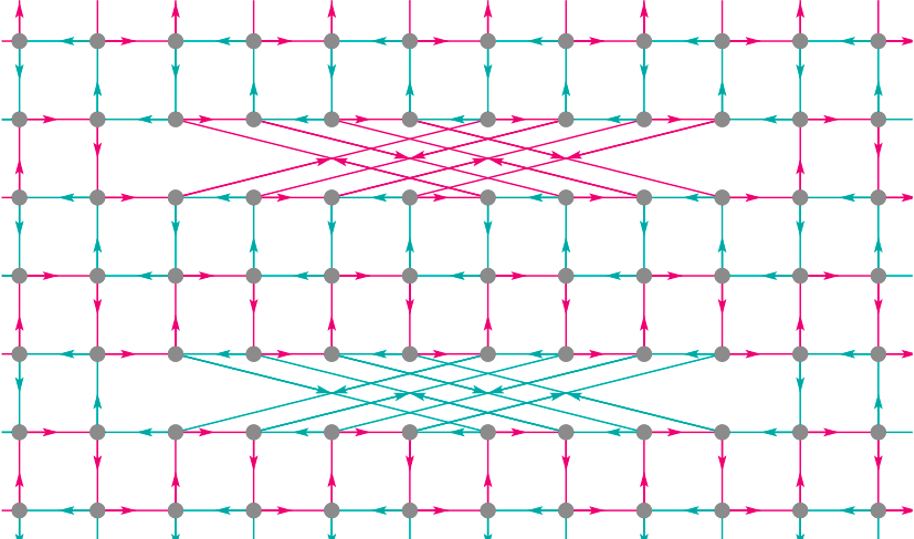
Figure 27: A closer view of the cable pattern: (a) Stitch instructions. (b) Simulation of the pattern. (c) Topology graph.

Figure 16 presents a row-by-row visualization of the Figure 15 swatch. Given an $n\times m$ stitch pattern, we can evaluate and visualize the topology of the pattern starting with the first row, followed by the first 2 rows, and so on. This visualization allows one to see the intermediate states of the data structure and the topology graph as the fabric is being knitted.

Figure 17 presents a stitch pattern that creates a “hole” in the swatch with transfer stitches that shift stitch loops away from each other. As the head nodes of the stitches are shifted to the left and right, the knit stitches above them are not properly formed and produce a “ladder” of unanchored CNs. These examples demonstrate that our approach is capable of generating unusual and possibly challenging yarn topologies by representing and aggregating local CN modifications.

Figures 21 and 21 present stitch patterns that include combinations of the Empty stitch (shown as an empty white cell) and transfer stitches in order to realize increases (widening) and decreases (narrowing) in the fabric. This allows TopoKnit to represent fabrics defined by more general, non-rectangular stitch patterns. Figures 24, 24 and 24 present slightly larger stitch patterns that include 3-level deep combinations of Knit, Tuck and Miss stitches, which demonstrate TopoKnit’s ability to determine non-local CN connectivity through the aggregation of local changes to CN state information. Figure 24 contains a pattern that transfers CNs to the left and then shifts them upwards two rows with recursive calls to FINAL_LOC_RECURSIVE.

Figure 25 presents two larger stitch patterns ($19\times 19$ stitches). The top example is a lace pattern and the bottom example is a cable. Figures 27 and 27 contain close-ups of the repeating patterns and allow for better assessment of the results. The topology graphs for these patterns were computed in approximately two seconds and demonstrate that TopoKnit is capable of rapidly processing stitch patterns for larger fabric swatches. Additionally we performed timing tests on a swatch that contains repeating blocks of the stitch pattern in Figure 15 in order to study the time complexity of TopoKnit’s evaluation algorithms. The values in Table 3 and the plot in Figure 14 demonstrate that the computation time needed to generate and evaluate the TopoKnit data structure increases linearly with the number of stitches in the modeled fabric. This linear behavior verifies that the individual evaluation algorithms execute in near-constant time.

As for handling the edges of the fabric in all of the examples, the CNs on the left and right boundaries are connected to the CNs either above or below them, depending on the parities of their $(i,j)$ IDs. For example, boundary CNs whose $(i,j)$ parities are the same, e.g. (odd,odd) or (even,even), connect to the CN above them in the grid with an outgoing yarn. CNs with differing $(i,j)$ parities are connected to the CN below them by an incoming yarn. As for the top and bottom boundaries, when a pattern is actually knitted cast-on and bind-off stitch combinations are added to the fabric to prevent the top and bottom edges from unraveling. TopoKnit includes the topology for these specialized stitches, but for visual simplicity they are not included in our graph visualizations.

8 Discussion

It should be noted that TopoKnit’s algorithms are based on several assumptions about the stitch patterns that define the analyzed fabric. Applying a few simple rules/constraints on a fabric’s stitch pattern guarantees the structural integrity (soundness) of the resulting fabric, and additionally ensures that our algorithms execute correctly. A structurally sound knitted fabric is one where all of its loops have been intertwined with another yarn. This property defines a knitted fabric that will not unravel. Using TopoKnit terminology, all CNs that define the head of a loop must eventually be actualized in a structurally sound fabric.

The restrictions imposed on the stitch patterns processed by TopoKnit are the following. 1) The stitches along the boundary of the pattern should be Knit or Purl stitches, or the increase and decrease combinations in Figures 21 and 21. 2) Empty stitches should only be defined on the “outside” of the stitch pattern, i.e. an Empty stitch should not be surrounded by non-Empty stitches. Note that an Empty stitch is different from an empty CN state, which can be surrounded by non-empty CNs, for example from a Miss stitch. 3) Transfer stitches should not shift their head nodes (their loops) outside of the boundary of the stitch pattern, i.e. to an Empty stitch. An example of a stitch pattern that is structurally unsound, violates the stitch rules and leads to an incorrectly evaluated topology is one with a Tuck stitch along the side boundary. This creates an unanchored CN along a side edge of the fabric, a situation that leads to stitch unraveling. While the rules limit which stitch patterns may be represented and evaluated by TopoKnit, they still allow for the modeling and analysis of a broad variety of structurally sound knitted fabrics.

We have described the query algorithms FINAL_LO-CATION (Algorithm 3) and ACNS_AT (Algorithm 5). These queries are central to the new TopoKnit query algorithms currently under development, which include determining the topological connections between CNs, the connections between locations, as well as the ordering of yarns at a certain $(i,j)$ location and at arbitrary spatial yarn crossings. CN and location connectivity is important to all flow simulations (heat, water and electrical current) conducted on a fabric substrate. Yarn stacking information would be additionally informative to electric circuit simulations over a knitted fabric, assuming that different yarn sections could have different conductivity / resistance.

For example, to compute the flow of water, heat or current through the yarns of a fabric, one needs to know how the yarn is in contact with itself. The exchange of heat, water, and current occurs where the yarn intertwines. The algorithm ACNS_AT and FINAL_LOCATION together provide the list of locations of these yarn intertwinings. The under-development CONNECTED_TO algorithm would provide the connections between the contacts needed to compute flow over the whole fabric. We also intend to integrate TopoKnit’s topology and yarn ordering information with the work of Wadekar et al. [30] to extend their yarn-level geometric models to complex knitted fabrics. These models support rapid evaluation of the mechanical properties of knitted fabrics.

It is important to note that the data structure and algorithms presented in this work have been based on high-level stitch commands that encapsulate multiple lower-level machine commands, thus, the space of knitted structures supported by TopoKnit is smaller than the space of structures generated from an arbitrary set of knitting machine commands (e.g. rack a needle bed, move a loop between beds, knit or drop a loop). These actions could be added to the data structure, but would require modifications of the algorithms. Also, initially we focused on stitch commands that create CN pairs only in one of the needle beds, thus, leaving out stitches that require CNs to be defined on both beds, such as the split stitch.

9 Conclusions and Future Work

In this paper we have proposed a process-oriented representation, TopoKnit, that defines a foundational data structure for representing the topology of the yarns in weft-knitted textiles. We have defined a process space that includes commonly used yarn-level operations, abstracted as mappings on yarn contact neighborhoods, produced by a weft-knitting knitting process. This space captures the essence of knitting processes in terms of their actions on yarns, but is independent of a particular machine architecture. In contrast to fabric space, the process space represents the structure of the fabric implicitly, eliminating the need for an explicit, fully-evaluated representation of its topology. Process space supports a concise, computationally efficient evaluation approach based on on-demand, near constant-time queries. We have defined the important features of this process space and designed a data structure to represent it and algorithms to evaluate it. Through the testing of more than 100 stitch patterns, we demonstrate the robustness and effectiveness of this representation scheme.

Work is underway to expand the scope, utility and applicability of TopoKnit. Given the information in the data structure, algorithms are being developed that can determine if a stitch pattern defines a structurally sound fabric. This feature would be useful for textile designers in that it would provide important information about the stitch pattern before attempting to manufacture it. Another test that could be easily implemented is related to manufacturability of a particular fabric. As noted in Section 6.1, most loops of yarn can only be stretched up to three needle locations away before either the yarn or the needle break. Flagging stitch combinations that produce excessive yarn stretching, and therefore threaten the integrity of the fabric or the knitting machine itself, is straightforward to realize.

As mentioned in Section 8, TopoKnit currently only supports the creation of CNs at a specific $(i,j)$ location on a single needle bed. However, the data structure can be extended to allow for creation of CNs on both beds at a specific $(i,j)$ location by including a separate CN array for each of the beds. This would also allow us to extend the set of stitch commands supported by TopoKnit. Our future work will also include algorithms to determine the stacking order of CNs at a specific $(i,j)$ location, as well, as the ordering of yarns where they cross in the fabric away from CN locations.

References

References

- [1] D. J. Spencer, Knitting technology: a comprehensive handbook and practical guide, Pergamon press, 1983.
- [2] D. Liu, D. Christie, B. Shakibajahromi, C. Knittel, N. Castaneda, D. Breen, G. Dion, A. Kontsos, On the role of material architecture in the mechanical behavior of knitted textiles, International Journal of Solids and Structures 109 (2017) 101–111.
- [3] D. Liu, B. Shakibajahromi, G. Dion, D. Breen, A. Kontsos, A computational approach to model interfacial effects on the mechanical behavior of knitted textiles, Journal of Applied Mechanics 85 (4) (2018) JAM–17–1584.
- [4] E. Tekerek, D. Liu, B. Wisner, M. Matthew, D. Breen, A. Kontsos, Integrated investigation of the role of 3D architecture in the mechanical behavior of knitted textiles, in: Proc. 18th European Conference on Composite Materials, 2018, pp. 2.15–10.
- [5] C. Knittel, D. Nicholas, R. Street, C. Schauer, G. Dion, Self-folding textiles through manipulation of knit stitch architecture, Fibers 3 (4) (2015) 575–587.
- [6] R. Vallett, C. Knittel, D. Christe, N. Castaneda, C. Kara, K. Mazur, D. Liu, A. Kontsos, Y. Kim, G. Dion, Digital fabrication of textiles: An analysis of electrical networks in 3D knitted functional fabrics, in: Micro-and Nanotechnology Sensors, Systems, and Applications IX, Vol. 10194, International Society for Optics and Photonics, 2017, p. 1019406.
- [7] C.-J. Hong, B.-J. Kim, Model-based simulation analysis of wicking behavior in hygroscopic cotton fabric, Journal of Fashion Business 20 (6) (2016) 66–78.
- [8] H. Shen, K. Xie, H. Shi, X. Yan, L. Tu, Y. Xu, J. Wang, Analysis of heat transfer characteristics in textiles and factors affecting thermal properties by modeling, Textile Research Journal 89 (21-22) (2019) 4681–4690.
- [9] F. Peirce, Geometrical principles applicable to the design of functional fabrics, Textile Research Journal 17 (3) (1947) 123–147.
- [10] G. Leaf, A. Glaskin, The geometry of a plain knitted loop, Journal of the Textile Institute Transactions 46 (9) (1955) T587–T605.
- [11] D. Munden, The geometry and dimensional properties of plain-knit fabrics, Journal of the Textile Institute Transactions 50 (7) (1959) T448–T471.
- [12] E. Cohen, R. Riesenfeld, G. Elber, Geometric Modeling with Splines, A K Peters, 2001.
- [13] A. Demiroz, T. Dias, A study of the graphical representation of plain-knitted structures part I: Stitch model for the graphical representation of plain-knitted structures, Journal of the Textile Institute 91 (4) (2000) 463–480.
- [14] A. Kurbak, O. Ekmen, Basic studies for modeling complex weft knitted fabric structures part I: A geometrical model for widthwise curlings of plain knitted fabrics, Textile Research Journal 78 (3) (2008) 198–208.
- [15] A. Kurbak, O. Kayacan, Basic studies for modeling complex weft knitted fabric structures part II: A geometrical model for plain knitted fabric spirality, Textile Research Journal 78 (4) (2008) 279–288.
- [16] A. Kurbak, Geometrical models for balanced rib knitted fabrics part i: Conventionally knitted 1 1 rib fabrics, Textile Research Journal 79 (5) (2009) 418–435.
- [17] W. Shanahan, R. Postle, A theoretical analysis of the plain-knitted structure, Textile Research Journal 40 (7) (1970) 656–665.
- [18] B. Hepworth, G. Leaf, The mechanics of an idealized weft-knitted structure, Journal of the Textile Institute 67 (7-8) (1976) 241–248.
- [19] S. De Jong, R. Postle, Energy analysis of mechanics of weft-knitted fabrics by means of optimal-control theory. part i: Nature of loop-interlocking in plain-knitted structure, Journal of The Textile Institute 68 (10) (1977) 307–315.
- [20] D. Semnani, M. Latifi, S. Hamzeh, A. Jeddi, A new aspect of geometrical and physical principles applicable to the estimation of textile structures: An ideal model for the plain-knitted loop, Journal of the Textile Institute 94 (3-4) (2003) 202–211.
- [21] S. De Jong, R. Postle, An energy analysis of the mechanics of weft-knitted fabrics by means of optimal-control theory. part ii: Relaxed-fabric dimensions and tensile properties of the plain-knitted structure, Journal of The Textile Institute 68 (10) (1977) 316–323.
- [22] K. Choi, T. Lo, An energy model of plain knitted fabric, Textile Research Journal 73 (8) (2003) 739–748.
- [23] K. F. Choi, T. Y. Lo, The shape and dimensions of plain knitted fabric: A fabric mechanical model, Textile Research Journal 76 (10) (2006) 777–786.
- [24] Y. Kyosev, Y. Angelova, R. Kovar, 3D modeling of plain weft knitted structures of compressible yarn, Research Journal of Textile and Apparel 9 (1) (2005) 88–97.
- [25] M. Sherburn, Geometric and mechanical modelling of textiles, Ph.D. thesis, University of Nottingham (2007).
- [26] H. Lin, X. Zeng, M. Sherburn, A. C. Long, M. J. Clifford, Automated geometric modelling of textile structures, Textile Research Journal 82 (16) (2012) 1689–1702.
- [27] M. Duhovic, D. Bhattacharyya, Simulating the deformation mechanisms of knitted fabric composites, Composites Part A: Applied Science and Manufacturing 37 (11) (2006) 1897–1915.
- [28] C. Knittel, Tools to predict and understand the self-folding behavior of knitted textiles, Ph.D. thesis, Drexel University (2019).
- [29] C. Knittel, M. Tanis, A. Stoltzfus, T. Castle, R. Kamien, G. Dion, Modelling textile structures using bicontinuous surfaces, Journal of Mathematics and the Arts 14 (4) (2020) 331–344.
- [30] P. Wadekar, P. Goel, C. Amanatides, G. Dion, R. Kamien, D. Breen, Geometric modeling of knitted fabrics using helicoid scaffolds, Journal of Engineered Fibers and Fabrics 15 (2020) 1–15.
- [31] P. Wadekar, L. Kapllani, C. Amanatides, G. Dion, R. Kamien, D. Breen, Geometric modeling of complex knitting stitches using a bicontinuous surface and its offsets, Under review.
- [32] M. Meissner, B. Eberhardt, The art of knitted fabrics, realistic & physically based modeling of knitted fabrics, Computer Graphics Forum (Proc. Eurographics) 17 (3) (1998) 355–362.
- [33] B. Eberhardt, M. Meissner, W. Strasser, Knit fabrics, in: D. House, D. Breen (Eds.), Cloth Modeling and Animation, AK Peters, 2000, Ch. 5, pp. 123–144.
- [34] B. Eberhardt, A. Weber, A particle system approach to knitted textiles, Computers & Graphics 23 (4) (1999) 599–606.
- [35] D. Breen, D. House, M. Wozny, A particle-based model for simulating the draping behavior of woven cloth, Textile Research Journal 64 (11) (1994) 663–685.
- [36] J. M. Kaldor, D. L. James, S. Marschner, Simulating knitted cloth at the yarn level, ACM Transactions on Graphics (Proc. SIGGRAPH) 27 (3) (2008) 65:1–65:9.
- [37] J. M. Kaldor, D. L. James, S. Marschner, Efficient yarn-based cloth with adaptive contact linearization, ACM Transactions on Graphics (Proc. SIGGRAPH) 29 (4) (2010) 105:1–105:10.
- [38] C. Yuksel, J. M. Kaldor, D. L. James, S. Marschner, Stitch meshes for modeling knitted clothing with yarn-level detail, ACM Transactions on Graphics (Proc. SIGGRAPH) 31 (3) (2012) 37:1–37:12.
- [39] K. Wu, X. Gao, Z. Ferguson, D. Panozzo, C. Yuksel, Stitch meshing, ACM Transactions on Graphics (Proc. SIGGRAPH) 37 (4) (2018) 130:1–130:14.
- [40] K. Wu, H. Swan, C. Yuksel, Knittable stitch meshes, ACM Transactions on Graphics 38 (1) (2019) 10:1–10:13.
- [41] J. Leaf, R. Wu, E. Schweickart, D. L. James, S. Marschner, Interactive design of periodic yarn-level cloth patterns, ACM Transactions on Graphics (Proc. SIGGRAPH Asia) 37 (6) (2018) 202:1–202:15.
- [42] M. Guo, J. Lin, V. Narayanan, J. McCann, Representing crochet with stitch meshes, Proc. ACM Symposium on Computational Fabrication (2020) 4:1–4:8.
- [43] Y. Igarashi, T. Igarashi, H. Suzuki, Knitting a 3D model, Computer Graphics Forum (Proc. Pacific Graphics) 27 (7) (2008) 1737–1743.
- [44] Y. Igarashi, T. Igarashi, H. Suzuki, Knitty: 3D modeling of knitted animals with a production assistant interface, in: Annex to Eurographics 2008 Proceedings, 2008, pp. 187–190.
- [45] J. McCann, L. Albaugh, V. Narayanan, A. Grow, W. Matusik, J. Mankoff, J. Hodgins, A compiler for 3D machine knitting, ACM Transactions on Graphics 35 (4) (2016) 49:1–49:11.
- [46] V. Narayanan, L. Albaugh, J. Hodgins, S. Coros, J. McCann, Automatic machine knitting of 3D meshes, ACM Transactions on Graphics 37 (3) (2018) 35:1–35:15.
- [47] J. Lin, V. Narayanan, J. McCann, Efficient transfer planning for flat knitting, in: Proc. 2nd ACM Symposium on Computational Fabrication, 2018, pp. 1:1–1:7.
- [48] V. Narayanan, K. Wu, C. Yuksel, J. McCann, Visual knitting machine programming, ACM Trans. Graph. 38 (4) (2019) 63:1–63:13.
- [49] M. Popescu, M. Rippmann, T. Van Mele, P. Block, Automated generation of knit patterns for non-developable surfaces, in: Humanizing Digital Reality, Springer, 2018, pp. 271–284.
- [50] A. Kaspar, L. Makatura, W. Matusik, Knitting Skeletons: A computer-aided design tool for shaping and patterning of knitted garments, in: Proc. ACM Symposium on User Interface Software and Technology, 2019, pp. 53–65.
- [51] G. Cirio, J. Lopez-Moreno, M. A. Otaduy, Yarn-level cloth simulation with sliding persistent contacts, IEEE Transactions on Visualization and Computer Graphics 23 (2) (2017) 1152–1162.
- [52] J. J. Casafranca, G. Cirio, A. Rodríguez, E. Miguel, M. A. Otaduy, Mixing yarns and triangles in cloth simulation, Computer Graphics Forum (Proc. Eurographics) 39 (2) (2020) 101–110.
- [53] R. M. Sánchez-Banderas, A. Rodríguez, H. Barreiro, M. A. Otaduy, Robust eulerian-on-lagrangian rods, ACM Transactions on Graphics 39 (4) (2020) 59:1–59:10.
- [54] J. Counts, Knitting with directed graphs, Master’s thesis, Massachusetts Institute of Technology (2018).
- [55] D. Liu, S. Koric, A. Kontsos, Parallelized finite element analysis of knitted textile mechanical behavior, Journal of Engineering Materials and Technology 141 (2) (2019) MATS–18–1132.
- [56] P. Wadekar, V. Perumal, G. Dion, A. Kontsos, D. Breen, An optimized yarn-level geometric model for finite element analysis of weft-knitted fabrics, Computer Aided Geometric Design 80 (2020) 101883.
- [57] T. Dinh, O. Weeger, S. Kaijima, S.-K. Yeung, Prediction of mechanical properties of knitted fabrics under tensile and shear loading: Mesoscale analysis using representative unit cells and its validation, Composites Part B: Engineering 148 (9) (2018) 81–92.
- [58] S. Poincloux, A.-B. Mokhtar, F. Lechenault, Geometry and elasticity of a knitted fabric, Physical Review X 8 (2) (2018) 021075.
- [59] D. Liu, S. Koric, A. Kontsos, A multiscale homogenization approach for architectured knitted textiles, Journal of Applied Mechanics 86 (11) (2019) JAM–19–1125.
- [60] G. Sperl, R. Narain, C. Wojtan, Homogenized yarn-level cloth, ACM Transactions on Graphics 39 (4) (2020) 48:1–48:16.