New results on inclusive $B\to X_{u}\ell\nu$ decay from the Belle experiment

Abstract

We report on the measurement of inclusive charmless semileptonic B decays $B\to X_{u}\ell\nu$. The analysis makes use of hadronic tagging and is performed on the full data set of the Belle experiment comprising 772 million $B\bar{B}$ pairs. In the proceedings, the preliminary results of measurements of partial branching fractions and the CKM matrix element $|V_{ub}|$ are presented.

1 Introduction

In the Standard Model of particle physics (SM), the Cabibbo-Kobayashi-Maskawa (CKM) matrix [1, 2] describes the quark mixing and accounts for $CP-$violation in the quark sector. One of the crucial tests of the SM is precise determination of the magnitude of the matrix elements. In $b-$flavor scope, the corresponding world averages of $|V_{ub}|$ from both exclusive and inclusive determinations [3] are

$$\begin{array}[]{l}\left|V_{ub}^{\text{excl. }}\right|=(3.67\pm 0.09\pm 0.12)\times 10^{-3},\\ \left|V_{ub}^{\text{incl. }}\right|=\left(4.32\pm 0.12_{-0.13}^{+0.12}\right)\times 10^{-3},\end{array}$$ (1)

where the uncertainties are from experiment and theory. The disagreement between them is about three standard deviations.

On the other hand, the experimental measurement of the inclusive semileptonic decay $B\to X_{u}\ell\nu$ is challenging due to the large background from the CKM-favoured $B\to X_{c}\ell\nu$ decay. Fig. 1 illustrates the $B\to X_{u}\ell\nu$ and $B\to X_{c}\ell\nu$ decays with the generator-level distributions in two important kinematic variables: the invariant mass of hadronic system $M_{X}$ and the lepton energy in the signal $B$ rest frame $E_{\ell}^{B}$. It’s shown that the clear separation of the signal decay is only possible in certain kinematic regions, e.g. the endpoint of lepton energy or the low $M_{X}$ region. The details of the reconstruction and separation strategy is described in Sec. 2. The preliminary results on the measured partial branching fractions and the $|V_{ub}|$ values are presented in Sec. 3.

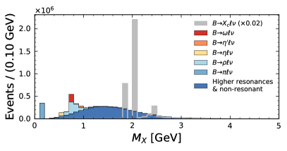
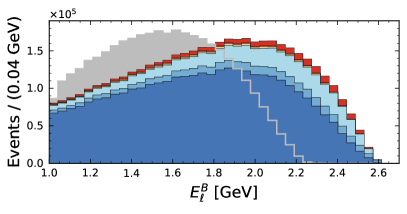
Figure 1: The generator-level $M_{X}$ and $E_{\ell}^{B}$ distributions of the $B\to X_{u}\ell\nu$ decay comparing to that of $B\to X_{c}\ell\nu$ decay. The $B\to X_{c}\ell\nu$ component (gray) is scaled down by a factor of 50 for illustration.

2 Analysis strategy

The data used in this analysis were recorded with the Belle detector [4] at the KEKB accelerator complex [5] with a center-of-mass energy of $\sqrt{s}=10.58$ GeV. The full data set contains an integrated luminosity of 711 fb^-1 and corresponds to 772 million $\Upsilon(4S)\to B\bar{B}$ events. The Monte Carlo (MC) simulated events are generated by EVTGEN [6] and the detector response is modeled using GEANT3 [7]. The signal $B\to X_{u}\ell\nu$ MC sample is a combination of resonances and non-resonant decay using a hybrid modelling approach [8, 9]. The non-resonant component is based on the theory calculation of Ref. [10] with the model parameters in the Kagan-Neubert scheme from Ref. [11].

The hadronic decays of one of the $B$ mesons are reconstructed via the full reconstruction algorithm [12] based on neural networks. In total, over 1104 decay cascades are considered and reconstructed. The efficiencies for charged and neutral $B$ mesons are $0.28\%$ and $0.18\%$, respectively [13]. The output classifier score of this algorithm presents the quality of the reconstructed candidates. We select the best candidate of $B_{\texttt{tag}}$ for each event. In addition, we require the beam-constrained mass $M_{\texttt{bc}}=\sqrt{(\sqrt{s}/2)^{2}-|\mathbf{p}_{\texttt{tag}}|^{2}}>5.27$ GeV to suppress continuum processes ($e^{+}e^{-}\to q\bar{q}$, $q=u,d,s,c$) and beam background.

All tracks and clusters not used in the construction of the $B_{\texttt{tag}}$ candidate are used to reconstruct the signal side. With the fully reconstructed four-momentum of $B_{\texttt{tag}}$ and the known beam-momentum, the signal $B$ rest frame can be defined as

$$p_{\mathrm{sig}}=p_{e^{+}e^{-}}-\left(\sqrt{m_{B}^{2}+\left|\mathbf{p}_{\mathrm{tag}}\right|^{2}},\mathbf{p}_{\mathrm{tag}}\right).$$ (2)

The signal lepton with $E_{\ell}^{B}=\left|\mathbf{p}_{\ell}^{\mathbf{B}}\right|>1$ GeV is used to identify the semileptonic decays. Here the small correction of the lepton mass term to the energy of the lepton is neglected. A veto on lepton-pair mass is applied to reject the lepton from $J/\psi$ decay and photon conversions. In addition, the charge of lepton is required to be opposite to $B_{\texttt{tag}}$ for the charged $B$ case. With the signal lepton selected, the four-momentum of hadronic system $p_{X}$ is defined as a sum of the four-momenta of tracks and clusters which are not involved in reconstructing the $B_{\texttt{tag}}$ and signal lepton. Furthermore, we reconstruct the missing mass squared and the four-momentum transfer squared $q^{2}$ as

$$\mathit{MM}^{2}=\left(p_{\mathrm{sig}}-p_{X}-p_{\ell}\right)^{2},\;\;q^{2}=\left(p_{\mathrm{sig}}-p_{X}\right)^{2}.$$ (3)

We utilise a machine learning based classification with boosted decision trees (BDTs) to separate the signal $B\to X_{u}\ell\nu$ decay from the background events which are dominated by $B\to X_{c}\ell\nu$. The feature variables used for training include $\mathit{MM}^{2}$, the number of charged kaons and $K_{s}^{0}$, the total charge of event, the vertex fit $\chi^{2}/\texttt{dof}$ between the hadronic system and signal lepton, and the $\mathit{MM}^{2}$ and angular information of a partially reconstructed $B\to D^{*}\ell\nu,D^{*}\to D\pi_{\texttt{slow}}$ decay with the slow pions candidates, where $p^{\texttt{cms}}_{\pi_{\texttt{slow}}}<0.22$ GeV. Due to the small difference between the masses of $D$ and $D^{*}$, the flight directions of the $\pi_{\texttt{slow}}$ and $D^{*}$ are strongly correlated and we estimate the energy of $D^{*}$ as $E_{D^{*}}\approx m_{D^{*}}\times E_{\pi_{\texttt{slow}}}/(m_{D^{*}}-m_{D})$. On the BDT classifier output, we choose a selection criteria that reject $98.1\%$ of $B\to X_{c}\ell\nu$ decays and retain $24.8\%$ of $B\to X_{u}\ell\nu$ signal decays. The selection efficiency on data is $2.3\%$.

In addition, the $B_{\texttt{tag}}$ reconstruction efficiency is calibrated using a data-driven approach described in Ref. [14]. The uncertainty of calibration is considered in systematics. We also apply a continuum efficiency correction to the simulated sample by comparing the difference to the number of reconstructed off-resonance events in data.

3 Partial branching fractions and $|V_{ub}|$ results

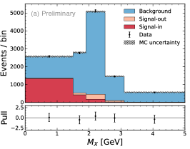
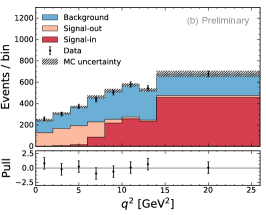
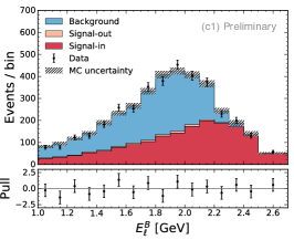
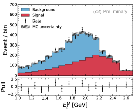
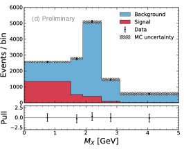
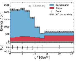
Figure 2: The post-fit distributions for various phase-space regions and kinematic variables. The distributions of the two-dimensional fit (d) are shown on the projections of $M_{X}$ and $q2$.

Fit	Fit variable	Phase-space region	$10^{3}\Delta\texttt{BF}$
(a)	$M_{X}$	$E^{B}_{\ell}>1$ GeV, $M_{X}<1.7$ GeV	$1.04\pm 0.04\pm 0.07$
(b)	$q^{2}$	$E^{B}_{\ell}>1$ GeV, $M_{X}<1.7$ GeV, $q^{2}>8$ GeV2	$0.70\pm 0.06\pm 0.09$
(c1)	$E^{B}_{\ell}$	$E^{B}_{\ell}>1$ GeV, $M_{X}<1.7$ GeV	$1.09\pm 0.05\pm 0.10$
(c2)	$E^{B}_{\ell}$	$E^{B}_{\ell}>1$ GeV	$1.66\pm 0.08\pm 0.17$
(d)	$M_{X}-q^{2}$	$E^{B}_{\ell}>1$ GeV	$1.56\pm 0.06\pm 0.12$

Table 1: The measured partial branching fractions for various phase-space regions. The first uncertainty is statistical and the second one is systematics.

A binned likelihood fit is performed to extract the signal yield, where the systematic uncertainties are incorporated via nuisance-parameter constraints. The fit uses MC templates for background, and for signal in and out-side of the selected phase-space regions. In total, we carry out five separate fits to measure the three partial branching fractions as summarised in Table 1. Fig. 2 shows the main fit results. The result based on the two-dimensional fit of $M_{X}$ and $q^{2}$, i.e. $\Delta\texttt{BF}=(1.56\pm 0.06\pm 0.12)\times 10^{-3}$, is in a good agreement with the one obtained by fitting the lepton spectrum, covering the same phase-space region. It also agrees well with the most precise measurement to date of this region  [15], where $\Delta\texttt{BF}=(1.55\pm 0.12)\times 10^{-3}$. For other phase-space regions, the measured partial branching fractions are also compatible with the previous measurements [16].

Based on the measured partial branching fractions, we calculate the $|V_{ub}|$ value with the theoretical input of decay rate as

$$\left|V_{ub}\right|=\sqrt{\frac{\Delta\mathcal{B}\left(B\rightarrow X_{u}\ell\nu\right)}{\tau_{B}\;\Delta\Gamma\left(B\rightarrow X_{u}\ell\nu\right)}}\;,$$ (4)

where the average $B$ meson lifetime is taken as $(1.579\pm 0.004)$ ps [17] and the state-of-the-art theory predictions on $\Delta\Gamma$ are listed in Table 2. Table 3 summarises the measured $|V_{ub}|$ values. To quote a single value for $|V_{ub}|$ we adapt the procedure of Ref. [17] and calculate a simple arithmetic average of the most precise determinations for the phase-space region $E^{B}_{\ell}>1$ GeV, obtaining

$$\left|V_{ub}\right|=(4.06\pm 0.09\pm 0.16\pm 0.15)\times 10^{-3}.$$ (5)

This value is smaller than the previous inclusive measurements of $|V_{ub}|$ in Ref. [18, 16]. The compatibility with the exclusive measurement of $|V_{ub}|$ in Eq.1 is 1.4 standard deviations; it is also compatible with the value expected from CKM unitarity from a global fit of Ref. [19] of $\left|V_{ub}\right|=(3.62^{+0.11}_{-0.08})\times 10^{-3}$ within 1.6 standard deviations.

Phase-space region	BLNP [20]	DGE [21, 22]	GGOU [23]	ADFR [24, 25]
$M_{X}<1.7\mathrm{GeV}$	$45.2_{-4.6}^{+5.4}$	$42.3_{-3.8}^{+5.8}$	$43.7_{-3.2}^{+3.9}$	$52.3_{-4.7}^{+5.4}$
$M_{X}<1.7\mathrm{GeV},q^{2}>8\mathrm{GeV}^{2}$	$23.4_{-2.6}^{+3.4}$	$24.3_{-1.9}^{+2.6}$	$23.3_{-2.4}^{+3.2}$	$31.1_{-2.6}^{+3.0}$
$E_{\ell}^{B}>1\mathrm{GeV}$	$61.5_{-5.1}^{+6.4}$	$58.2_{-3.0}^{+3.6}$	$58.5_{-2.3}^{+2.7}$	$61.5_{-5.1}^{+5.8}$

Table 2: The theory predicted decay rates in the three phase-space regions ($\texttt{ps}^{-1}$).

Fit	$10^{3}|V_{ub}|^{\texttt{BLNP}}$	$10^{3}|V_{ub}|^{\texttt{DGE}}$	$10^{3}|V_{ub}|^{\texttt{GGOU}}$	$10^{3}|V_{ub}|^{\texttt{ADFR}}$
(a)	$3.81_{-0.08,-0.13,-0.21}^{+0.08,+0.13,+0.21}$	$3.99_{-0.08,-0.14,-0.26}^{+0.08,+0.14,+0.20}$	$3.88_{-0.08,-0.14,-0.16}^{+0.08,+0.13,+0.15}$	$3.55_{-0.07,-0.12,-0.17}^{+0.07,+0.12,+0.17}$
(b)	$4.35_{-0.18,-0.28,-0.28}^{+0.18,+0.26,+0.26}$	$4.27_{-0.18,-0.28,-0.21}^{+0.17,+0.26,+0.18}$	$4.36_{-0.18,-0.28,-0.27}^{+0.18,+0.27,+0.24}$	$3.77_{-0.16,-0.24,-0.17}^{+0.15,+0.23,+0.17}$
(c1)	$3.90_{-0.10,-0.18,-0.21}^{+0.09,+0.17,+0.21}$	$4.08_{-0.10,-0.19,-0.26}^{+0.10,+0.18,+0.20}$	$3.97_{-0.10,-0.19,-0.16}^{+0.09,+0.18,+0.15}$	$3.63_{-0.09,-0.17,-0.17}^{+0.09,+0.16,+0.17}$
(c2)	$4.14_{-0.10,-0.22,-0.20}^{+0.10,+0.20,+0.18}$	$4.25_{-0.10,-0.22,-0.12}^{+0.10,+0.21,+0.11}$	$4.24_{-0.10,-0.22,-0.10}^{+0.10,+0.21,+0.09}$	$4.14_{-0.10,-0.22,-0.18}^{+0.10,+0.20,+0.18}$
(d)	$4.01_{-0.08,-0.16,-0.19}^{+0.08,+0.15,+0.18}$	$4.12_{-0.09,-0.16,-0.12}^{+0.08,+0.16,+0.11}$	$4.11_{-0.09,-0.16,-0.09}^{+0.08,+0.16,+0.08}$	$4.01_{-0.08,-0.16,-0.18}^{+0.08,+0.15,+0.18}$

Table 3: The extracted $|V_{ub}|$ values based on four theoretical inputs on the decay rates. The first uncertainty is statistical, the second one is systematic and the last term comes from the corresponding theory calculation.

4 Summary and outlook

The preliminary results are obtained with the hadronic tagged analysis based on the full Belle data set. The measured partial branching fractions for the three phase-space regions are compatible with the previous measurements. The preliminary $|V_{ub}|$ value extracted in this analysis is larger but compatible with the exclusive determination within 1.4 standard deviations. Based on this preliminary result, the final analysis will incorporate a few modifications, including the aspects of increasing the simulated sample size and considering additional systematics accounting for the signal modeling. The separate-mode branching fractions for $B^{+}/B^{0}$ and $e/\mu$ will be also provided.

References

- Cabibbo [1963] N. Cabibbo, Phys. Rev. Lett. 10, 531 (1963).
- Kobayashi and Maskawa [1973] M. Kobayashi and T. Maskawa, Prog. Theor. Phys. 49, 652 (1973).
- Amhis et al. [2019] Y. S. Amhis et al. (HFLAV), (2019), arXiv:1909.12524 [hep-ex] .
- Abashian et al. [2002] A. Abashian et al., Nucl. Instrum. Meth. A479, 117 (2002), also see detector section in J. Brodzicka et al., Prog. Theor. Exp. Phys. 2012, 04D001 (2012).
- Kurokawa and Kikutani [2003] S. Kurokawa and E. Kikutani, Nucl. Instr. and. Meth. A499, 1 (2003), and other papers included in this Volume; T. Abe et al., Prog. Theor. Exp. Phys. 2013, 03A001 (2013) and references therein.
- Lange [2001] D. J. Lange, Nucl. Instr. and. Meth. A462, 152 (2001).
- Brun et al. [1987] R. Brun, F. Bruyant, M. Maire, A. C. McPherson, and P. Zanarini, CERN-DD-EE-84-1 (1987).
- Ramirez et al. [1990] C. Ramirez, J. F. Donoghue, and G. Burdman, Phys. Rev. D 41, 1496 (1990).
- Prim et al. [2020] M. Prim et al. (Belle Collaboration), Phys. Rev. D 101, 032007 (2020).
- De Fazio and Neubert [1999] F. De Fazio and M. Neubert, JHEP 06, 017 (1999).
- Buchmuller and Flacher [2006] O. Buchmuller and H. Flacher, Phys. Rev. D 73, 073008 (2006), arXiv:hep-ph/0507253 .
- Feindt et al. [2011] M. Feindt, F. Keller, M. Kreps, T. Kuhr, S. Neubauer, D. Zander, and A. Zupanc, Nucl. Instrum. Meth. A 654, 432 (2011).
- Bevan et al. [e 95] A. Bevan et al., Eur. Phys. J. C 74, 3026 (2014, Page 95).
- Glattauer et al. [2016] R. Glattauer et al. (Belle Collaboration), Phys. Rev. D93, 032006 (2016).
- Lees et al. [2017] J. Lees et al. (BaBar Collaboration), Phys. Rev. D 95, 072001 (2017).
- Lees et al. [2012] J. Lees et al. (BaBar Collaboration), Phys. Rev. D 86, 032004 (2012).
- Zyla et al. [2020] P. Zyla et al. (Particle Data Group), Prog. Theor. Exp. Phys. 2020 083C01 (2020).
- Urquijo et al. [2010] P. Urquijo et al. (Belle Collaboration), Phys. Rev. Lett. 104, 021801 (2010).
- Charles et al. [2005] J. Charles, A. Hocker, H. Lacker, S. Laplace, F. Le Diberder, J. Malcles, J. Ocariz, M. Pivk, and L. Roos (CKMfitter Group), Eur. Phys. J. C 41, 1 (2005).
- Lange et al. [2005] B. O. Lange, M. Neubert, and G. Paz, Phys. Rev. D 72, 073006 (2005).
- Andersen and Gardi [2006] J. R. Andersen and E. Gardi, JHEP 01, 097 (2006).
- Gardi [2008] E. Gardi, Frascati Phys. Ser. 47, 381 (2008).
- Gambino et al. [2007] P. Gambino, P. Giordano, G. Ossola, and N. Uraltsev, JHEP 10, 058 (2007).
- Aglietti et al. [2009] U. Aglietti, F. Di Lodovico, G. Ferrera, and G. Ricciardi, Eur. Phys. J. C 59, 831 (2009).
- Aglietti et al. [2007] U. Aglietti, G. Ferrera, and G. Ricciardi, Nucl. Phys. B 768, 85 (2007).