Implementing Approximate Bayesian Inference using Adaptive Quadrature: the aghq Package

Alex Stringer Implementing Adaptive Quadrature for Bayesian Inference: the aghq Package aghq: Adaptive Quadrature for Bayesian Inference The aghq package for implementing approximate Bayesian inference using adaptive quadrature is introduced. The method and software are described, and use of the package in making approximate Bayesian inferences in several challenging low- and high-dimensional models is illustrated. Examples include an infectious disease model; an astrostatistical model for estimating the mass of the Milky Way; two examples in non-Gaussian model-based geostatistics including one incorporating zero-inflation which is not easily fit using other methods; and a model for zero-inflated, overdispersed count data. The aghq package is especially compatible with the popular TMB interface for automatic differentiation and Laplace approximation, and existing users of that software can make approximate Bayesian inferences with aghq using very little additional code. The aghq package is available from CRAN and complete code for all examples in this paper can be found at https://github.com/awstringer1/aghq-software-paper-code. bayesian, quadrature, optimization, spatial bayesian, quadrature, optimization, spatial University of Toronto, Toronto, Canada
Centre for Global Health Research, St. Michael’s Hospital, Toronto, Canada

1 Introduction

Bayesian inferences are based upon summaries of a posterior distribution. Computing this distribution and summaries of it requires evaluating a difficult integral—called the normalizing constant or marginal likelihood—and this computation is infeasible to do exactly in all but the simplest of problems. Modern approaches for inference in a wide range of models are based on approximations to the posterior. These approximations, in turn, often rely on approximations to the normalizing constant.

Quadrature refers to the approximation of an integral of a function (called the integrand) using a finite weighted sum of evaluations of that function. A quadrature rule is a set of nodes at which the function is to be evaluated and weights by which the function evaluations are to be multiplied when summing. There is a rich literature on quadrature rules and their properties from a numerical analysis perspective (numint) as well as on their use in statistical problems (evansintegrations), and this literature may be drawn upon when choosing a rule to use for integrating a chosen function. Of particular importance is ensuring that the quadrature rule places high weight on evaluations which are near to where the function takes its largest values. This is necessary to obtain an accurate approximation to the integral.

Because the normalizing constant is an integral, in principle any quadrature technique may be used to approximate it and (hence) make approximate Bayesian inferences. However, the posterior is defined by a particular model and prior and its location and shape are random variables which vary with the data. In practice, therefore, the region where the posterior takes its largest values will change with different models, priors, and data. It follows that no fixed quadrature rule can be expected to work well for all posterior distributions, even those obtained from the same model and prior but different datasets. Care is required when applying quadrature in the contex of Bayesian inference.

Adaptive Quadrature techniques take any fixed quadrature rule and shift and scale its nodes and weights according to the mode and curvature of the integrand, attempting to automatically focus attention on the region where the integrand takes its largest values. The goal of adaptive quadrature is to obtain an accurate and useful approximation to a wider variety of integrals than any single fixed quadrature rule can. Application of adaptive quadrature to the approximation of the normalizing constant is therefore a potentially useful techinque for making approximate Bayesian inferences.

Both the theoretical and practical advantages of adaptive quadrature as a tool for making approximate Bayesian inferences have recently been studied by aghqus. These authors show that adaptation of a broad class of fixed quadrature rules using the posterior mode and curvature yields a method for making approximate Bayesian inferences that has compelling asymptotic properties under standard conditions on the model. They also motivate the use of adaptive quadrature in challenging Bayesian inference problems through several examples, which are considered in greater computational detail in §3 and §4 of the present manuscript.

When the fixed quadrature rule used is Gauss-Hermite Quadrature (GHQ), the corresponding adaptive rule is called Adaptive Gauss-Hermite Quadrature (AGHQ). Since AGHQ was introduced in the statistical literature (nayloradaptive; laplace; adaptive_GH_1994; adaptive_GH_2020) it has been used in a variety of applications including latent variable models (aghqmle) and as the default option for approximating the likelihood in Generalized Linear Mixed Models in the glmer function in the popular lme4 package (lme4). While the theoretical analysis of aghqus applies to any quadrature rule which satisfies certain properties, their examples focus on AGHQ. This choice is partly due to some desirable properties of GHQ (§LABEL:sec:background), the connection of AGHQ with the Laplace approximation, and the prevalence of AGHQ in the existing literature. This focus on AGHQ is the case for the remainder of this paper as well, although other quadrature rules including those based on sparse grids and sampling-based evaluations could in principle replace GHQ in all of what follows and may be implemented in ongoing future releases of the aghq package.

Like all quadrature techniques, GHQ and hence AGHQ are only directly useful for models in which the dimension of the parameter space is not too large. However, one interesting property of AGHQ specifically is that it recovers the Laplace approximation when run with only a single quadrature point, avoiding the unfavourable increase in computation time that usually occurs with increasing dimension. When the dimension of the parameter space is large, several applications of AGHQ with different numbers of quadrature points can be applied, recovering the marginal Laplace approximation of laplace. This approach is available in the aghq package and is applied to high-dimensional latent Gaussian models (inla) in §4.1 and extended latent Gaussian models (lgmsplit; maxandsmooth; noeps) in §4.2. The aghq therefore provides users with a template for making approximate Bayesian inferences in a wide range of challenging, high-dimensional models.

There are several existing packages which implement Adaptive Quadrature to some extent, however they are all either too specific or too general for the present setting, applying only to specific models or lacking functions for using the results to make approximate Bayesian inferences. For example, the fastGHQuad package (fastghquad) implements AGHQ for general scalar functions only, requires the user to supply their own mode and curvature information, and does not include any functions for post-processing the results. The GLMMadaptive package (glmmadaptive) handles optimization and has a formula interface and an API for post-processing model results, but only fits Generalized Linear Mixed Models with independent random effects. The LaplacesDemon package provides an option to use AGHQ to improve moment estimation in models fit either with MCMC or a Laplace Approximation, but does not offer further use of the technique. Finally, the popular INLA package (inla; inlasoftware) makes approximate Bayesian inferences for a class of latent Gaussian additive models, implementing several types of adaptive quadrature among a rich collection of approximations. The interface is aimed at a general scientific audience and comparatively less of a focus is placed on specialists who wish to implement their own models, although doing so is possible for models which are compatible with the underlying methodology.

In this paper the new aghq package is introduced. The aghq package contains an interface for approximating the normalizing constant using AGHQ, and making approximate Bayesian inferences based on the result. For users who are implementing their own priors and likelihoods, the aghq package is simple to use, yet flexible enough to make approximate Bayesian inferences in a wide range of problems not covered by existing software. Standard print, summary, and plot methods are provided for output objects of class aghq. A flexible interface for taking aghq objects and computing moments, quantiles, and marginal densities/distribution functions is also provided. Further, in certain cases, fast independent samples from the approximate posterior are provided as well, enabling the estimation of complicated posterior summaries not covered by other methods in the package.

While not a requirement, the aghq package has been designed to work especially well in combination with the popular TMB package (tmb) which offers an interface for automatic differentiation and unnormalized marginal Laplace approximations in R. Use of TMB handles the computation of the two derivatives required to implement Adaptive Quadrature and which can otherwise be challenging to obtain in the types of complicated models that aghq was designed to fit. It also provides an automatic Laplace approximate marginal posterior and an efficient, exact gradient of this quantitity. Implementing approximate Bayesian inference for complicated additive models (§2.6) is straightforward using TMB in combination with aghq, as demonstrated in §4. Users who already have their unnormalized log-posteriors coded in TMB can made approximate Bayesian inferences of a form similar to inla and noeps using only two additional lines of code.

Further, while unrelated to the aghq package, it is important to point out that use of TMB to implement the unnormalized log-posterior further allows implementation of MCMC for the same model using no additional code with the tmbstan package (tmbstan), allowing comparison of AGHQ and MCMC for problems in which the latter is computationally feasible. Therefore the use of TMB embeds aghq within a comprehensive framework for performing the challenging computations associated with making approximate Bayesian inferences. All of the examples in this paper include comparisons to MCMC and all but one are implemented in TMB, illustrating this approach.

The remainder of this paper is organized as follows. In §2 the basic use of the aghq package is described in detail using the simple example from the simulations in aghqus. In §LABEL:sec:background the necessary background on AGHQ is provided, including explicit formulas and a brief statement of some relevant mathematical properties. In §3 two examples from aghqus are implemented using the aghq package, providing users with a detailed template describing the use of the package for making approximate Bayesian inferences. In §4 the Generalized Linear Geostatistical Model (GLGM) considered by geostatsp and prevmap is implemented using aghq, and then extended to fit the much more challenging zero-inflated binomial geostatistical model described by geostatlowresource. In §LABEL:sec:glmmTMB aghq is used to make approximate Bayesian inferences in a situation where other authors (glmmTMB) have already implemented the model in TMB, which is a main intended use case of the package. The paper concludes in §LABEL:sec:discussion with a discussion of impact and future work.

2 Basic Use

In this section the basic use of the aghq package is demonstrated by way of analyzing a simple example in which the answer is known. Detailed discussion of Bayesian inference and quadrature in R deferred to §LABEL:sec:background. All notation and terms are defined in detail in that section.

The following conjugate model is used in simulations by aghqus:

$$Y_{i}\ |\ \lambda \overset{ind}{\sim}\text{Poisson}(\lambda),i\in[n],$$ (1)

$$\lambda \sim\text{Exponential}(1),\lambda>0,$$

$$\implies\lambda\ |\ \boldsymbol{Y} \sim\text{Gamma}\left(1+\sum_{i=1}^{n}y_{i},n+1\right).$$

The empirical accuracy of the method will depend on how close to log-quadratic the posterior distribution is, with the method being more accurate for posteriors which are closer to being log-quadratic. While the constraint that $\lambda>0$ does not pose any barrier to application of AGHQ in theory, box constraints of this type are often obvious indicators that a parameter transformation may yield a posterior that is closer to being log-quadratic, and hence for which AGHQ will provide more accurate results (nayloradaptive). Here we set $\theta=\log\lambda$, perform the normalization on this scale, and then use the features of the aghq package to make inferences for $\lambda=e^{\theta}$. It is important to reiterate that this step is not strictly necessary, but is a good strategy to employ in practice.

The goal of the analysis is to approximate

$$\pi(\boldsymbol{Y})=\int_{0}^{\infty}\frac{\lambda^{\sum_{i=1}^{n}Y_{i}}e^{-(n+1)\lambda}}{\prod_{i=1}^{n}Y_{i}!}d\lambda=\frac{\Gamma\left(\sum_{i=1}^{n}Y_{i}+1\right)}{(n+1)^{\sum_{i=1}^{n}Y_{i}+1}\prod_{i=1}^{n}Y_{i}!},$$ (2)

and then make Bayesian inferences based on $\pi(\lambda|\boldsymbol{Y})$ (§LABEL:sec:background). First, install and load the aghq package:

R> # Install stable version from CRAN: R> # install.packages("aghq") R> # or development version from github: R> # devtools::install_github("awstringer1/aghq") R> library(aghq)

Simulate some data from the true data generating process:

R> set.seed(84343124) R> y <- rpois(10,5) # True lambda = 5, n = 10

The main function in the aghq package is aghq::aghq(). The user supplies a list containing the log-posterior and its first two derivatives:

R> logpithetay <- function(theta,y) + sum(y) * theta - (length(y) + 1) * exp(theta) - sum(lgamma(y+1)) + theta + R> objfunc <- function(x) logpithetay(x,y) R> objfuncgrad <- function(x) numDeriv::grad(objfunc,x) R> objfunchess <- function(x) numDeriv::hessian(objfunc,x) R> # Now create the list to pass to aghq() R> funlist <- list( + fn = objfunc, + gr = objfuncgrad, + he = objfunchess + ) as well as the number of quadrature points, $k$, and a starting value for the optimization. Inference using AGHQ is then performed: R> # AGHQ with k = 3 R> # Use theta = 0 as a starting value R> thequadrature <- aghq::aghq(ff = funlist,k = 3,startingvalue = 0) The object thequadrature has class aghq, with summary and plot methods:

R> # Not shown R> # summary(thequadrature) R> # plot(thequadrature)

The object thequadrature contains all quantities necessary for computation of approximate moments of any function $g(\theta)$, approximate quantiles and marginal probability densities and cumulative distribution functions of $\theta$ and any monotone transformation of it (including for each parameter in multidimensional models), and exact samples from these approximate marginals using the inverse CDF method/probability integral transform. Note that much of this information is displayed easily using the summary and plot methods for objects of class aghq. How to obtain these quantities one at a time, using the interface for aghq objects provided by the aghq package, is now described.

R> # The normalized posterior at the adapted quadrature points: R> thequadrature$normalized_{p}osterior$nodesandweights theta1 weights logpost logpost_normalized 1 1.246489 0.2674745 -23.67784 -0.3566038 2 1.493925 0.2387265 -22.29426 1.0269677 3 1.741361 0.2674745 -23.92603 -0.6047982 R> # The log normalization constant: R> thequadrature$normalized_{p}osterior$lognormconst [1] -23.32123 R> # Compare to the truth: R> lgamma(1 + sum(y)) - (1 + sum(y)) * log(length(y) + 1) - sum(lgamma(y+1)) [1] -23.31954 R> # The mode found by the optimization: R> thequadrature$optresults$mode [1] 1.493925 R> # The true mode: R> log((sum(y) + 1)/(length(y) + 1)) [1] 1.493925

Of course, in most problems, the true mode and normalizing constant won’t be known.

The aghq package provides further routines for computing moments, quantiles, marginal probability densities and cumulative distribution functions (including for monotone transformations), and exact independent samples from the approximate marginal posteriors. These routines are especially useful when working with transformations like we are in the example, since interest here is in the original parameter $\lambda=e^{\theta}$. The functions are all S3 methods with a method for objects of class aghq. These are as follows:

• compute_pdf_and_cdf: compute the density and cumulative distribution function for a marginal posterior distribution of $\theta$ and (optionally) a smooth monotone transformation of that variable;

• compute_moment: compute the posterior moment of any function of $\theta$;

• compute_quantiles: compute posterior quantiles for a marginal posterior distribution.

For multidimensional parameters, all of these functions work on the associated multiple marginal posterior distributions, without any additional input from the user.

To compute the approximate marginal posterior for $\lambda$, $\widetilde{\pi}_{\texttt{AGHQ}}(\lambda|\boldsymbol{Y})$, we first compute the marginal posterior for $\theta$ and then transform:

$$\widetilde{\pi}_{\texttt{AGHQ}}(\lambda|\boldsymbol{Y})=\widetilde{\pi}_{\texttt{AGHQ}}(\theta|\boldsymbol{Y})\left\lvert\frac{\mathrm{d}\theta}{\mathrm{d}\lambda}\right\rvert.$$ (3)

The aghq::compute_pdf_and_cdf() function has an option, transformation, which allows the user to specify a parameter transformation that they would like the marginal density of. The user specifies functions fromtheta and totheta which convert from and to the transformed scale (on which quadrature was done), and the function returns the marginal density on both scales, making use of a numerically differentiated jacobian. This is all done as follows:

R> # Compute the pdf for theta R> transformation <- list(totheta = log,fromtheta = exp) R> pdfwithlambda <- compute_pdf_and_cdf( + thequadrature, + transformation = transformation + )[[1]] R> lambdapostsamps <- + sample_marginal(thequadrature,1e04,transformation = transformation)[[1]] R> head(pdfwithlambda,n = 2) theta pdf cdf transparam pdf_transparam 1 0.9990534 0.008604132 0.000000e+00 2.715710 0.003168281 2 1.0000441 0.008809832 8.728201e-06 2.718402 0.003240813 R> # Plot the approximate density R> # and samples along with the true posterior R> with(pdfwithlambda, + hist(lambdapostsamps,breaks = 50,freq = FALSE,main = "",xlab = expression(lambda)) + lines(transparam,pdf_transparam) + lines(transparam,dgamma(transparam,1+sum(y),1+length(y)),lty=’dashed’) + )

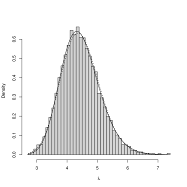
Figure 1: Approximate (—, ${\color[rgb]{.75,.75,.75}\blacksquare}$) and true (- - -) posterior $\pi(\lambda|\boldsymbol{Y})$ in the example of §2.

The need to index element [[1]] from the output here feels messy, but is necessary to keep the interface consistent between single- and multi-dimensional models.

We may compute the posterior mean of $\lambda=e^{\theta}$, $\mathop{\mathrm{\mathbb{E}}}(\lambda|\boldsymbol{Y})$ by using the compute_moment function:

R> # Posterior mean for lambda = exp(theta) R> compute_moment(thequadrature$normalized_{p}osterior,+ff=function(x)exp(x))\CodeOutput[1]4.454407\CodeInput R>#Comparetothetruth:R>(sum(y)+1)/(length(y)+1)\CodeOutput[1]4.454545Theargument\texttt{ff}ispassedthrough\texttt{match.fun()}sothat\texttt{ff = exp}and\texttt{ff = 'exp'}arealsobothvalidinput.\par Quantilesarecomputedusingthe\texttt{compute\_quantiles()}function.Forexample,togetthe$1%$and$99%$percentilesaswellasthemedianandfirstandthirdquartilesof$λ$:\par\CodeChunk\CodeInput R>#QuantilesR>compute_{q}uantiles(+thequadrature,+q=c(.01,.25,.50,.75,.99),+transformation=transformation+)[[1]]\CodeOutput 13.1664694.0005444.4040814.8483236.149735\CodeInput R>#Thetruth:R>qgamma(c(.01,.25,.50,.75,.99),1+sum(y),1+length(y))\CodeOutput[1]3.1088964.0104304.4242794.8656836.067076\par Theestimationofquantiles,especiallyextremequantiles,ismuchmoredifficultthanthatofmoments,andthisisreflectedinthesmalldifferencesinaccuracyobservedbetweenthetwointhisexample.\par$

In this section, the underlying methodology of AGHQ is reviewed with an emphasis on computational details. The notation follows aghqus who describe the methodological background in much greater detail.

2.1 Bayesian Inference

Let $\boldsymbol{\theta}\in\Theta\subseteq\mathbb{R}^{d}$ denote a parameter, let $\pi(\boldsymbol{\theta})$ denote its prior density, and let $\boldsymbol{Y}=\left\{Y_{i}:i\in[n]\right\}$ denote a sample with likelihood $\pi(\boldsymbol{Y}|\boldsymbol{\theta})$. Bayesian inferences are made from summaries of the posterior distribution:

$$\pi(\boldsymbol{\theta}|\boldsymbol{Y})=\frac{\pi^{*}(\boldsymbol{\theta},\boldsymbol{Y})}{\int_{\Theta}\pi^{*}(\boldsymbol{\theta},\boldsymbol{Y})\mathrm{d}\boldsymbol{\theta}},$$ (4)

where $\pi^{*}(\boldsymbol{\theta},\boldsymbol{Y})=\pi(\boldsymbol{Y}|\boldsymbol{\theta})\pi(\boldsymbol{\theta})$. The denominator of (4) is called the normalizing constant, denoted by $\pi(\boldsymbol{Y})$:

$$\pi(\boldsymbol{Y})=\int_{\Theta}\pi^{*}(\boldsymbol{\theta},\boldsymbol{Y})\mathrm{d}\boldsymbol{\theta},$$ (5)

and this is infeasible to compute exactly unless the model is very simple.

Inferences are made from summaries of $\pi(\boldsymbol{\theta}|\boldsymbol{Y})$, which are themselves (intractable) integrals. The posterior mean of any function $f:\Theta\to\mathbb{R}$ is

$$\mathop{\mathrm{\mathbb{E}}}[f(\boldsymbol{\theta})|\boldsymbol{Y}]=\int_{\Theta}f(\boldsymbol{\theta})\pi(\boldsymbol{\theta}|\boldsymbol{Y})d\boldsymbol{\theta},$$

and for any $t\in[d],\alpha\in[0,1]$ the marginal posterior $\alpha$-quantile of $\theta_{t}$ is the number $q_{t}^{\alpha}$ which satisfies

$$\int_{\mathbb{R}^{d-1}\times(-\infty,q_{t}^{\alpha})}\pi(\boldsymbol{\theta}|\boldsymbol{Y})d\boldsymbol{\theta}_{-t}d\theta_{t}=\alpha.$$

The posterior mean $\mathop{\mathrm{\mathbb{E}}}(\theta_{t}|\boldsymbol{Y})$ or median $q_{t}^{0.5}$ are common point estimates of the components $\theta_{t}$, and the posterior standard deviation or extreme quantiles are commonly used to quantify uncertainty. The aghq package provides a framework in which $\pi(\boldsymbol{Y})$ is approximated using AGHQ and approximate Bayesian inferences are made using such summary statistics calculated from the corresponding approximation to $\pi(\boldsymbol{\theta}|\boldsymbol{Y})$.

2.2 Quadrature

For any function $f:\mathbb{R}^{d}\to\mathbb{R}$, a quadrature approximation with $k\in\mathbb{N}$ points to its integral is given by the weighted sum:

$$\int_{A}f(\boldsymbol{x})\mathrm{d}\boldsymbol{x}\approx\sum_{\boldsymbol{x}\in\mathcal{Q}(d,k)}f(\boldsymbol{x})\omega(\boldsymbol{x}),$$ (6)

where $A\subseteq\mathbb{R}^{d}$ is any set, $\mathcal{Q}(d,k)\subset\mathbb{R}^{d}$ is the set of nodes, and $\omega:\mathcal{Q}(d,k)\to\mathbb{R}$ are weights. In R, quadrature is performed using the flexible interface provided by the mvQuad package, which computes the nodes and weights for different quadrature rules with $d,k\in\mathbb{N}$. For example, with $d=1,k=3$, GHQ is implemented as:

R> # Integrate exp(-x^2) on (-Inf,Inf) R> f <- function(x) exp(-(x^2)/2) R> # Define a grid for Gauss-Hermite quadrature R> # with k = 3 points R> gg <- mvQuad::createNIGrid(1,"GHe",3) R> # Perform the quadrature R> mvQuad::quadrature(f,gg) [1] 2.51 R> # True value is sqrt(2pi) R> sqrt(2*pi) [1] 2.51

When $d>1$, such univariate rules are extended to multiple dimensions, and there are a number of ways in which this can be done. Here we focus only on product rule extensions, in which the nodes are repeated in each dimension and the weights multiplied, defining $\mathcal{Q}(d,k)=\mathcal{Q}(1,k)^{d}$ and $\omega(\boldsymbol{x})=\prod_{j=1}^{d}\omega(x_{j})$. Using this technique with $\left\lvert\mathcal{Q}(1,k)\right\rvert=k$ points per dimension and a $d$-dimensional integrand therefore requires $\left\lvert\mathcal{Q}(d,k)\right\rvert=k^{d}$ function evaluations, and this is computationally expensive. Methods based on sparse grids (sparsegrids) or employing more detailed computations to compute the nodes and weights (designedquadrature) may alleviate this challenge somewhat, however these are not yet implemented in the aghq package. The present approach to inference in high-dimensional additive models is discussed in §2.6 with examples in §4.

2.3 Gauss-Hermite Quadrature

Gauss-Hermite Quadrature (GHQ; numint) is a useful quadrature rule based on the theory of polynomial interpolation. Define the Hermite polynomials

$$H_{k}(x)=(-1)^{k}e^{x^{2}/2}\frac{d^{k}}{dx^{k}}e^{-x^{2}/2}$$ (7)

where $k\in\mathbb{N}$. The GHQ nodes and weights with $k$ quadrature points are:

$$\mathcal{Q}(1,k) =\left\{x\in\mathbb{R}:H_{k}(x)=0\right\},$$ (8)

$$\omega(x) =\frac{k!}{H_{k+1}(x)^{2}\times\phi(x)},j\in[k],$$

where $\phi(\cdot)$ is a standard normal density. Some interesting properties of GHQ are as follows: (numint):

1. $x=0$ is a node if and only if $k$ is odd;

2. $-x$ is a node if and only $x$ is;

3. $\omega_{j}>0$ for each $j\in[k]$;

4. for a polynomial $P_{\alpha}(x)$ of degree $\alpha\leq 2k-1$,

   $$\int_{\mathbb{R}}P_{\alpha}(x)\phi(x)\mathrm{d}x=\sum_{x\in\mathcal{Q}(1,k)}P_{\alpha}(x)\phi(x)\omega(x),$$

   and no other quadrature rule with the same number of points $k$ can obtain this exactness property for polynomials of higher degree;

5. for any suitable function $f(\cdot)$, there exists some $\xi\in\mathbb{R}$ such that

   $$\int_{\mathbb{R}}f(x)\phi(x)\mathrm{d}x\equiv\sum_{x\in\mathcal{Q}(1,k)}f(x)\phi(x)\omega(x)+f^{(2k)}(\xi)E_{k},$$

   where $E_{k}$ is an error term depending on $k$ with $E_{k}\downarrow 0$ as $k\uparrow\infty$.

The natural equivalents of several of these properties hold in multiple dimensions, although formally stating them requires more advanced notation and definitions. See aghqus for further detail.

2.4 Adaptive Gauss-Hermite Quadrature

The unnormalized posterior $\pi^{*}(\boldsymbol{\theta},\boldsymbol{Y})$ has a location and curvature which vary stochastically with $\boldsymbol{Y}$, and no fixed quadrature rule will perform well for all datasets and models. A rule which adapts to the changing shape and location of $\pi^{*}(\boldsymbol{\theta},\boldsymbol{Y})$ is desirable. The Laplace approximation (laplace) is possibly the most well-known example of such a technique, in which $\pi^{*}(\boldsymbol{\theta},\boldsymbol{Y})$ is approximated using an appropriately shifted and scaled Gaussian distribution and this is used to approximate $\pi(\boldsymbol{Y})$. This is closely related to a more general discussion of adaptive quadrature techniques which I now briefly describe.

Adaptive quadrature techniques shift and scale the nodes and weights of a given fixed quadrature rule according to the mode and curvature of $\pi^{*}(\boldsymbol{\theta},\boldsymbol{Y})$. Define

$$\widehat{\boldsymbol{\theta}} =\text{argmax}_{\boldsymbol{\theta}}\log\pi^{*}(\boldsymbol{\theta},\boldsymbol{Y}),$$ (9)

$$\boldsymbol{H} =-\partial^{2}_{\boldsymbol{\theta}}\log\pi^{*}(\widehat{\boldsymbol{\theta}},\boldsymbol{Y}),$$

$$\boldsymbol{H}^{-1} =\boldsymbol{L}\boldsymbol{L}^{\tiny{\texttt{T}}},$$

where $\boldsymbol{L}$ is the (unique) lower Cholesky triangle. For a given rule with nodes $\mathcal{Q}(d,k)$ and weights $\omega$, the corresponding adaptive quadrature approximation to $\pi(\boldsymbol{Y})$ is:

$$\widetilde{\pi}(\boldsymbol{Y})=\left\lvert\boldsymbol{L}\right\rvert\sum_{\boldsymbol{x}\in\mathcal{Q}(d,k)}\pi(\boldsymbol{Lx}+\widehat{\boldsymbol{\theta}},\boldsymbol{Y})\omega(\boldsymbol{x}).$$ (10)

When the fixed quadrature rule is GHQ, the method is called Adaptive Gauss-Hermite Quadrature (AGHQ; nayloradaptive; adaptive_GH_1994; adaptive_GH_2020; aghqus), and the corresponding approximation is denoted $\widetilde{\pi}_{\texttt{AGHQ}{}}(\boldsymbol{Y})$. This is the focus of the remainder of this paper. Some interesting properties of AGHQ are as follows (although they may be shared by other adaptive rules as well):

1. The mode $\widehat{\boldsymbol{\theta}}$ is a quadrature point if and only if $k$ is odd;

2. When $k=1$, AGHQ is a Laplace approximation, providing a principled link between adaptive quadrature in low and high dimensions (§2.6, §4);

3. When $k>1$, AGHQ achieves higher-order asymptotic accuracy: aghqus show that if $\widetilde{\pi}_{\texttt{AGHQ}}(\boldsymbol{Y})$ is an AGHQ approximation to $\pi(\boldsymbol{Y})$ using $k$ points, then

   $$\widetilde{\pi}_{\texttt{AGHQ}}(\boldsymbol{Y})=\pi(\boldsymbol{Y})\left[1+\mathcal{O}_{p}\left(n^{-\lfloor(k+2)/3\rfloor}\right)\right],$$ (11)

   where the convergence is in probability measured with respect to the distribution of $\boldsymbol{Y}$. Table 1 shows the asymptotic accuracy achieved for selected $k$. Note that the well-known $n^{-1}$ rate for the Laplace approximation is recovered when $k=1$. Note that their analysis applies to any rule that satisfies property 4. from §2.3 (polynomial exactness), not only GHQ.

$k$	Rate
1	$\mathcal{O}_{p}\left(n^{-1}\right)$
3	$\mathcal{O}_{p}\left(n^{-1}\right)$
5	$\mathcal{O}_{p}\left(n^{-2}\right)$
7	$\mathcal{O}_{p}\left(n^{-3}\right)$
9	$\mathcal{O}_{p}\left(n^{-3}\right)$
11	$\mathcal{O}_{p}\left(n^{-4}\right)$
13	$\mathcal{O}_{p}\left(n^{-5}\right)$
15	$\mathcal{O}_{p}\left(n^{-5}\right)$

Table 1: Asymptotic rates for AGHQ

2.5 Posterior summaries

With the AGHQ approximation $\widetilde{\pi}_{\texttt{AGHQ}}(\boldsymbol{Y})$ to $\pi(\boldsymbol{Y})$, the approximate posterior density is

$$\widetilde{\pi}_{\texttt{AGHQ}}(\boldsymbol{\theta}|\boldsymbol{Y})=\frac{\pi^{*}(\boldsymbol{\theta},\boldsymbol{Y})}{\widetilde{\pi}_{\texttt{AGHQ}}(\boldsymbol{Y})},$$ (12)

and, by definition, satisfies

$$\left\lvert\boldsymbol{L}\right\rvert\sum_{\boldsymbol{x}\in\mathcal{Q}(d,k)}\widetilde{\pi}_{\texttt{AGHQ}}(\boldsymbol{Lx}+\widehat{\boldsymbol{\theta}}|\boldsymbol{Y})\omega(\boldsymbol{x})=1.$$ (13)

For any function $f:\mathbb{R}^{d}\to\mathbb{R}$, the posterior moment $\mathop{\mathrm{\mathbb{E}}}[f(\boldsymbol{\theta})|\boldsymbol{Y}]$ may be approximated by

$$\mathop{\mathrm{\mathbb{E}}}[f(\boldsymbol{\theta})|\boldsymbol{Y}]\approx\left\lvert\boldsymbol{L}\right\rvert\sum_{\boldsymbol{x}\in\mathcal{Q}(d,k)}f(\boldsymbol{Lx}+\widehat{\boldsymbol{\theta}})\widetilde{\pi}_{\texttt{AGHQ}}(\boldsymbol{Lx}+\widehat{\boldsymbol{\theta}}|\boldsymbol{Y})\omega(\boldsymbol{x}),$$ (14)

and this is what the compute_moment() function does (§2). Note that this is not an application of AGHQ to the integral defining this expectation; laplace (among others) discuss approximating such summaries which occur as ratios of integrals, however approximations of this type are not implemented in the aghq package. The re-use of the AGHQ points and weights in computation of moments is not yet covered by theory, but appears empirically accurate in applications (§3).

Marginal posteriors and quantiles are more difficult to compute, as described in detail by nayloradaptive and aghqus. The challenge is that the adaptive quadrature rule is only defined at specific points of the form $\boldsymbol{Lx}+\widehat{\boldsymbol{\theta}},\boldsymbol{x}\in\mathcal{Q}(d,k)$, and these points are not on a regular grid. It is therefore only straightforward to evaluate marginal posteriors at $k$ distinct points, and this only works for the first element of $\boldsymbol{\theta}$. To mitigate these challenges, the parameter vector has to be re-ordered and the joint normalization re-computed for each desired marginal distribution, although the optimization results are reused. A polynomial or spline-based interpolant to these points is then used for plotting and computing quantiles. See aghqus for further detail. As described in §2, the aghq package handles these computations for the user through the compute_pdf_and_cdf() and compute_quantiles() functions.

2.6 High-dimensional additive models

A very important use case and motivation for development of the aghq package is the fitting high-dimensional additive models by combining the Laplace ($k=1$) and AGHQ ($k>1$) approximations. This is inspired by the popular INLA approach of inla for latent Gaussian models, and further explored by casecrossover; noeps for the broader class of extended latent Gaussian models introduced by lgmsplit; maxandsmooth. The applications of casecrossover; noeps include semi-parametric regression with multinomial response, analysis of aggregated spatial point process data, survival analysis with spatially-varying hazard, and an astrophysical measurement error model for estimating the mass of the Milky Way. Other examples include non-Gaussian model-based geostatistics with zero-inflated observations (aghqus), and large-scale spatio-temporal models (inlamra) where the comparison to INLA is made more explicitly. Here the core approach to inference using aghq is described, with details to follow for the individual models fit in §4.

Consider a model with parameter $(\boldsymbol{W},\boldsymbol{\theta})\in\mathbb{R}^{m}\times\mathbb{R}^{d}$ where $m\gg d$. It is assumed that $d$ is small enough to reasonably apply AGHQ with $k>1$ to integrals involving $\boldsymbol{\theta}$ (§2, §LABEL:sec:background), but that $m$ is so large as to render this computationally infeasible for integrals involving $\boldsymbol{W}$, even if using sparse grids or other multidimensional extensions more efficient than the product rule we use here. The posteriors of interest are:

$$\pi(\boldsymbol{\theta}|\boldsymbol{Y}) \propto\int_{\mathbb{R}^{m}}\pi(\boldsymbol{W},\boldsymbol{\theta},\boldsymbol{Y})d\boldsymbol{W},$$ (15)

$$\pi(\boldsymbol{W}|\boldsymbol{Y}) =\int_{R^{d}}\pi(\boldsymbol{W}|\boldsymbol{\theta},\boldsymbol{Y})\pi(\boldsymbol{\theta}|\boldsymbol{Y})d\boldsymbol{\theta}.$$

Applying AGHQ with $k=1$ to $\pi(\boldsymbol{\theta}|\boldsymbol{Y})$ yields the (unnormalized) marginal Laplace approximation of laplace, $\widetilde{\pi}_{\texttt{LA}}(\boldsymbol{\theta},\boldsymbol{Y})$, and then normalizing this using AGHQ with $k>1$ gives:

$$\widetilde{\pi}_{\texttt{LA}}(\boldsymbol{\theta}|\boldsymbol{Y})=\frac{\widetilde{\pi}_{\texttt{LA}}(\boldsymbol{\theta},\boldsymbol{Y})}{\left\lvert\boldsymbol{L}\right\rvert\sum_{\boldsymbol{x}\in\mathcal{Q}(d,k)}\widetilde{\pi}_{\texttt{LA}}(\boldsymbol{Lx}+\widehat{\boldsymbol{\theta}},\boldsymbol{Y})\omega(\boldsymbol{x})}.$$ (16)

A suitable Gaussian approximation is used for $\pi(\boldsymbol{W}|\boldsymbol{\theta},\boldsymbol{Y})\approx\widetilde{\pi}_{\texttt{G}}(\boldsymbol{W}|\boldsymbol{\theta},\boldsymbol{Y})$. The AGHQ nodes and weights are reused in the final approximation:

$$\pi(\boldsymbol{W}|\boldsymbol{Y})\approx\widetilde{\pi}(\boldsymbol{W}|\boldsymbol{Y})=\left\lvert\boldsymbol{L}\right\rvert\sum_{\boldsymbol{x}\in\mathcal{Q}(d,k)}\widetilde{\pi}_{\texttt{G}}(\boldsymbol{W}|\boldsymbol{Lx}+\widehat{\boldsymbol{\theta}},\boldsymbol{Y})\widetilde{\pi}_{\texttt{LA}}(\boldsymbol{Lx}+\widehat{\boldsymbol{\theta}}|\boldsymbol{Y})\omega(\boldsymbol{x}).$$ (17)

Inferences for $\boldsymbol{W}$ and any function of it are made by drawing exact posterior samples from the mixture-of-Gaussians approximation $\widetilde{\pi}(\boldsymbol{W}|\boldsymbol{Y})$. The full algorithm is given by noeps. The INLA approach of inla then involves approximating the marginal posteriors $\pi(W_{j}|\boldsymbol{Y}),j\in[m]$ using a further Laplace approximation, but this is not yet implemented in aghq.

The aghq package contains an interface for performing these challenging computations. The normalized marginal Laplace approximation $\widetilde{\pi}_{\texttt{LA}}(\boldsymbol{\theta}|\boldsymbol{Y})$ is obtained using aghq::marginal_laplace(). This function internally defines $\log\widetilde{\pi}_{\texttt{LA}}(\boldsymbol{\theta},\boldsymbol{Y})$ using aghq::laplace_approximation() and then calls aghq::aghq(). However, it uses numerical derivatives of $\log\widetilde{\pi}_{\texttt{LA}}(\boldsymbol{\theta},\boldsymbol{Y})$, and hence requires repeated optimizations of $\log\pi(\boldsymbol{W},\boldsymbol{\theta},\boldsymbol{Y})$ at great computational expense. The use of marginal_laplace() is recommended for simpler models in which this strategy is feasible.

The recommended general approach to implementing Equation (17) is to implement $-\log\pi(\boldsymbol{W},\boldsymbol{\theta},\boldsymbol{Y})$ as a function template in the popular TMB package (tmb) and turn on the random flag for $\boldsymbol{W}$. This provides $-\log\widetilde{\pi}_{\texttt{LA}}(\boldsymbol{\theta},\boldsymbol{Y})$ and its exact gradient automatically, avoiding repeated expensive optimizations over $\boldsymbol{W}$. The aghq::marginal_laplace_tmb() function accepts such a template from TMB and utilizes these features, leading to more efficient computations for normalizing $\log\widetilde{\pi}_{\texttt{LA}}(\boldsymbol{\theta},\boldsymbol{Y})$ using AGHQ. An added benefit of this feature of the aghq package is that the many users who are already using TMB to make approximate Bayesian inferences using its built in Gaussian approximations can begin making more accurate approximate Bayesian inferences using AGHQ with almost no additional code.

Both aghq::marginal_laplace() and aghq::marginal_laplace_tmb() return objects inheriting from classes aghq and marginallaplace. Inferences for $\boldsymbol{\theta}$ are therefore made using all the same functions as described in §2, which automatically work on $\widetilde{\pi}_{\texttt{LA}}(\boldsymbol{\theta}|\boldsymbol{Y})$. Sample-based inferences for $\boldsymbol{W}$ are made using the aghq::sample_marginal() function which acts on marginallaplace objects and draws fast, exact samples from $\widetilde{\pi}(\boldsymbol{W}|\boldsymbol{Y})$ by making use of quantities previously computed and saved by aghq::marginal_laplace*. These samples are then used to estimate any posterior summary of interest. The entire approach is best illustrated through the examples of §4 and §LABEL:sec:glmmTMB, which despite their complexity all require remarkably little code to implement beyond the likelihood and priors themselves with to the aghq package.

3 Examples, low dimensions

In this section the two low-dimensional examples considered by aghqus are implemented using aghq. The use of aghq is highlighted and results are compared to the Gaussian approximation returned by TMB, as well as MCMC through tmbstan. All code for these examples is available from https://github.com/awstringer1/aghq-software-paper-code; only brief illustrative code is included in the text here.

3.1 Infectious disease models

epi implement MCMC for a Susceptible, Infectious, Removed (SIR) model for the spread of infectious disease in the EpiILMCT package. Here we illustrate how to use the aghq package to fit this model as done by aghqus. We compare to MCMC using the tmbstan package, finding that AGHQ produces results much faster than MCMC with little loss in accuracy for this simple model.

We consider their example of an outbreak of the Tomato Spotted Wilt Virus in $n=520$ plants, of which $n_{0}=327$ were infected. For observed infection times $\boldsymbol{I}=\left\{I_{i}:i\in[n]\right\}$ with $I_{1}\leq\cdots\leq I_{n_{0}}$ and $I_{i}=\infty,i=n_{0}+1,\ldots,n$, as well as removal times $\boldsymbol{R}=\left\{R_{i},i\in[n]\right\}$, the likelihood is

$$\pi(\boldsymbol{I},\boldsymbol{R}|\alpha,\beta)=\prod_{j=2}^{n_{0}}\left(\sum_{i:I_{i}<I_{j}\leq R_{i}}\lambda_{ij}\right)\exp\left\{-\sum_{i=1}^{n_{0}}\sum_{j=1}^{n}[\text{min}(R_{i},I_{j})-\text{min}(I_{i},I_{j})]\lambda_{ij}\right\},$$ (18)

where $\lambda_{ij}=\alpha d_{ij}^{-\beta}$ with $d_{ij}$ the Euclidean distance between plants $i$ and $j$. Independent $\text{Exponential}(0.01)$ priors are placed on the parameters of interest $(\alpha,\beta)$, and quadrature is performed on the transformed scale with $\boldsymbol{\theta}=(\log\alpha,\log\beta)$. See aghqus and epi for further information.

To implement AGHQ for this problem using the aghq package, we define a list of functions ff which compute the log-posterior and its first two derivatives, and then call the aghq function as in §2:

R> library(TMB) R> data("tswv", package = "EpiILMCT") R> # Create the functions R> ff <- TMB::MakeADFun(…) R> # Do the quadrature R> quadmod <- aghq(ff,9,c(0,0),control = default_control(negate = TRUE))

The template returned by TMB::MakeADFun() returns the negated unnormalized log-posterior $-\log\pi(\boldsymbol{\theta},\boldsymbol{Y})$, which is required to use tmbstan. The control = default_control(negate = TRUE) option tells aghq() to account for this internally.

We can compute marginal moments, quantiles, and densities of $\alpha$ and $\beta$:

R> # Mean of alpha and beta R> compute_moment(quadmod,function(x) exp(x)) [1] 0.01203082 1.30371767 R> # Quantiles of alpha and beta R> posttrans <- list(totheta = log,fromtheta = exp) R> compute_quantiles(quadmod,transformation = posttrans) [[1]] 2.50.007570042 0.016617720

[[2]] 2.50.981385 1.582341 R> # Marginal densities R> quaddens <- compute_pdf_and_cdf(quadmod,posttrans) Joint posterior moments may also be approximated: for example, for two plants which are $d_{ij}=2$ units apart, the infectivity rate is $\lambda_{ij}=\alpha\cdot 2^{-\beta}$. We can approximate $\mathop{\mathrm{\mathbb{E}}}(\lambda_{ij}|\boldsymbol{Y})$ as: R> compute_moment( + quadmod, + function(x) exp(x)[1] * 2^(-exp(x)[2]) + ) [1] 0.004804631 The length of the return value of compute_moment() equals the length of its second argument, the function whose moment is being approximated. The value of each component is the approximate posterior moment of that component.

Finally, marginal posterior samples of size $M$ are obtained from $\widetilde{\pi}_{\texttt{AGHQ}{}}(\alpha|\boldsymbol{Y})$ and $\widetilde{\pi}_{\texttt{AGHQ}{}}(\beta|\boldsymbol{Y})$ using the univariate inverse CDF/probability integral transform: R> quadsamps <- sample_marginal(quadmod,M) These could be used to estimate any marginal posterior summary of interest.

Figure 2 shows the AGHQ approximate marginal posteriors along with those obtained using tmbstan. Table 2 shows various summary statistics obtained using both methods, including the KS statistics obtained by running ks.test() on the MCMC and AGHQ marginal posterior samples for both variables. The results based on AGHQ are very close to those obtained using MCMC. The runtime for AGHQ was $0.59$ seconds, compared to 330.88 seconds using MCMC with four parallel chains of 10,000 iterations each (including warmup) and all the default settings. Since the number of iterations must be chosen and this changes the runtime of MCMC, we base our conclusions about relative runtimes off of the observation that the time it took to fit the model using AGHQ is sufficient to run only $0.59\times 10000/330.88=17.84$ iterations of MCMC using the chosen settings. It appears that AGHQ results in faster inferences with little loss of accuracy in this example.

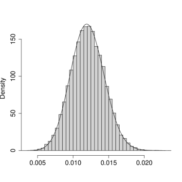
(a) $\alpha$

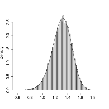
(b) $\beta$

Figure 2: Approximate posteriors using AGHQ (—) and MCMC (${\color[rgb]{.75,.75,.75}\blacksquare}$) for the infectious disease model example of §3.1.

	$\alpha$		$\beta$
	AGHQ	MCMC	AGHQ	MCMC
$\operatorname{\mathbb{E}}(\cdot|\boldsymbol{Y})$	0.0120	0.0121	1.30	1.31
$\text{SD}(\cdot|\boldsymbol{Y})$	0.00232	0.00235	0.153	0.155
$\widetilde{q}^{0.025}$	0.00757	0.0755	0.981	0.982
$\widetilde{q}^{0.975}$	0.0166	0.0167	1.58	1.59
$\operatorname{\mathbb{E}}(\alpha\cdot 2^{-\beta}|\boldsymbol{Y})$	0.00480	0.00481	-	-
KS(AGHQ,MCMC)	0.0195		0.0235

Table 2: Comparison of approximate posterior summary statistics obtained using AGHQ and MCMC for the infectious disease model example of §3.1.

3.2 Estimating the mass of the Milky Way Galaxy

Astrophysicists are interested in estimating the mass of the Milky Way Galaxy. gwen2 describe a statistical model which relates multivariate position/velocity measurements of star clusters orbiting the Galaxy to parameters which in turn determine its mass according to a physical model. Their interest is in assessing the impact of various prior choices and data inclusion rules on inferences, and they fit and assess many models using MCMC. aghqus implement the model using AGHQ. Here, the use of the aghq package to fit this model is demonstrated. The high accuracy attained (in theory) by AGHQ is shown to produce results that are much closer to the MCMC samples returned by tmbstan than a simpler Gaussian approximation to the posterior used in TMB. Further, the aghq package gives these more accurate results using about the same amount of code and with similar runtime to TMB.

In this example the optimization required to implement AGHQ is more challenging than in the example of §3.1. The aghq package accomodates more difficult optimization problems by allowing the user to perform the optimization outside and pass in the results, and this feature is illustrated here. Some current limitations of the methods underpinning the aghq package are also illustrated through the estimation and quantification of uncertainty for a complicated nonlinear, transdimensional posterior summary using AGHQ and MCMC.

Let $\boldsymbol{Z}_{i}=(z_{i1},\ldots,z_{i4})$ denote the position and three-component velocity measured relative to the sun (Heliocentric measurements) for the $i^{th}$ star cluster, $i\in[n],n=70$. These are what is actually measured. These measurements are then transformed into position and radial and tangential velocity measurements relative to the centre of the Galaxy (Galactocentric measurements) $\boldsymbol{Y}_{i}=(y_{i1},y_{i2},y_{i3})$. The probability density for $\boldsymbol{Y}_{i}$ is

$$f(\boldsymbol{Y}_{i};\boldsymbol{\Xi})=\frac{L_{i}^{-2\beta}\mathcal{E}_{i}^{\frac{\beta(\gamma-2)}{\gamma}+\frac{\alpha}{\gamma}-\frac{3}{2}}\Gamma\left(\frac{\alpha}{\gamma}-\frac{2\beta}{\gamma}+1\right)}{\sqrt{8\pi^{3}2^{-2\beta}}\Psi_{0}^{-\frac{2\beta}{\gamma}+\frac{\alpha}{\gamma}}\Gamma\left(\frac{\beta(\gamma-2)}{\gamma}+\frac{\alpha}{\gamma}-\frac{1}{2}\right)},$$ (19)

where $L_{i}=y_{i1}y_{i3}$ and $\mathcal{E}_{i}=\Psi_{0}y_{i1}^{1-\gamma}-(y_{i2}^{2}+y_{i3}^{2})/2$. The parameters $\boldsymbol{\Xi}=(\Psi_{0},\gamma,\alpha,\beta)$ determine the mass of the Galaxy at radial distance $r$ kiloparsecs (kpc) from Galaxy centre as:

$$M_{\boldsymbol{\Xi}}(r)=\Psi_{0}\gamma r^{1-\gamma},$$ (20)

according to a physical model, and inference is done for $M_{\boldsymbol{\Xi}}(r)$ at various values of $r$.

The parameters are subject to nonlinear and box constraints:

$$\alpha >\gamma,\qquad\alpha>\beta(2-\gamma)+\frac{\gamma}{2},\qquad\mathcal{E}_{i}>0,i\in[n],$$ (21)

$$\alpha \geq 3,\qquad 1\leq\Psi\leq 200,\qquad 0.3\leq\gamma\leq 0.7,\qquad-0.5\leq\beta\leq 1.$$

Uniform priors on these ranges are used for $\Psi,\gamma,\beta$, and a $\text{Gamma}(1,4.6)$ prior is used for $\alpha-3$. We perform quadrature on the transformed scale $\boldsymbol{\theta}=(\theta_{1},\theta_{2},\theta_{3},\theta_{4})$ with

$$\theta_{1}=\log\left(-\log\left[\frac{\Psi-1}{200-1}\right]\right), \qquad\theta_{2}=\log\left(-\log\left[\frac{\gamma-0.3}{0.7-0.3}\right]\right),$$ (22)

$$\theta_{3}=\log(\alpha-3), \qquad\theta_{4}=\log\left(-\log\left[\frac{\beta+0.5}{1+0.5}\right]\right).$$

This transformation enhances the spherical symmetry of the posterior and we find it to improve the stability of the optimization and the empirical quality of the AGHQ approximation, as suggested by nayloradaptive. The nonlinear constraints remain, however, and none of the built-in optimizers provided by aghq handle this. For this reason, optimization in this example is performed manually using the much more substantial optimization interface from the ipoptr package (ipopt), and these results are passed to aghq::aghq(). This works as follows:

R> library(TMB) R> data("gcdatalist",package = "aghq") R> # Negated un-normalized log-posterior and its derivatives R> ff <- TMB::MakeADFun(…,ADreport = FALSE) R> # Nonlinear constraints and their jacobian R> Es <- TMB::MakeADFun(…,ADreport = TRUE) R> # Optimization R> ipopt_result <- ipoptr::ipoptr(…) R> useropt <- list( + ff = list( + fn = function(theta) -1*ff$fn(theta),+gr=function(theta)-1*ff$gr(theta), + he = function(theta) -1*ff$he(theta)+),+mode=ipopt_{r}esult$solution, + hessian = ff$he(ipopt_{r}esult$solution) + ) R> # Quadrature R> astroquad <- aghq( + ff,5,thetastart,optresults = useropt,control = default_control(negate=TRUE) + ) A Gaussian approximation $\widetilde{\pi}_{\texttt{G}}(\boldsymbol{\theta}|\boldsymbol{Y})$ uses a mean equal to $\widehat{\boldsymbol{\theta}}$ and covariance matrix equal to $\boldsymbol{H}^{-1}$, with approximate marginal posteriors obtained from the corresponding marginal Gaussian distributions. The information obtained from TMB: R> tmbsd <- TMB::sdreport(ff) is also present in the aghq output: R> # Matches tmbsd$par.fixedR>astroquad$optresults$modeR>#Matchessqrt(diag(tmbsd$cov.fixed)) R> sqrt(diag(solve(astroquad$optresults$hessian))) Figure 3 shows the approximate marginal posterior distributions of the four model parameters, obtained using MCMC, TMB and AGHQ, and Table 3 shows the estimated KS distance between the MCMC results and samples from the approximate posteriors using AGHQ and TMB. In general, AGHQ is much closer to MCMC than the Gaussian approximation; this is especially evident for $\alpha$, which has a sharply skewed posterior and for which the Gaussian approximation is very inaccurate, especially in the tails, where this would have an effect on calculation of credible intervals. The runtime of AGHQ was 1.40 seconds, taking 1.02 seconds for optimization using ipopt and 0.38 seconds for quadrature; TMB required no additional time beyond the optimization. The MCMC was run under the same conditions as Example 3.1 and had a runtime of 21.9 seconds, meaning that AGHQ could be run in the time it takes to run 640 MCMC iterations, while TMB takes the same time as 468 iterations.

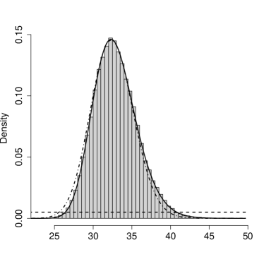
(a) $\Psi_{0}$

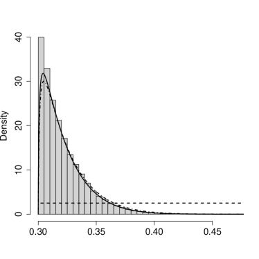
(b) $\gamma$

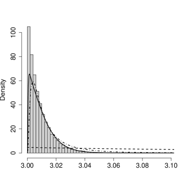
(c) $\alpha$

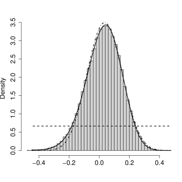
(d) $\beta$

Figure 3: Approximate posteriors using AGHQ (—), TMB (-$\cdot$-) and MCMC (${\color[rgb]{.75,.75,.75}\blacksquare}$) for the Galaxy mass estimation example of §3.2.

Param.	AGHQ	TMB
$\Psi_{0}$	0.010	0.044
$\gamma$	0.0073	0.031
$\alpha$	0.035	0.16
$\beta$	0.0099	0.025

Table 3: Estimated KS distances between the MCMC results and those from AGHQ and TMB for the Galaxy mass estimation example of §3.2.

The interest in this example is in the cumulative mass profile $M_{\boldsymbol{\Xi}}(r)$ at a variety of values of distance from the centre of the Galaxy, $r$, in kiloparsecs (kPc). Estimates of the posterior mean and standard deviation of this quantity are easily obtained using aghq::compute_moment(): R> # Cumulative mass profile R> Mr <- function(r,theta) + p = get_psi0(theta[1]) + g = get_gamma(theta[2]) + # Manual unit conversion into "mass of one trillion suns" + g*p*r^(1-g) * 2.325e09 * 1e-12 + R> # Posterior mean mass at 100 kPc from centre, for example: R> compute_moment(astroquad,function(x) Mr(100,x)) [1] 0.5592737 Because $M_{\boldsymbol{\Xi}}(r)$ is a nonlinear, transdimensional summary of $\boldsymbol{\theta}$, neither approximate credible intervals nor sample-based inference are available options in the current release of aghq. The best we can currently do with the aghq is estimate its mean and standard deviation and use the latter to quantify uncertainty in the former, which effectively amounts to assuming a Gaussian posterior for $M_{\boldsymbol{\Xi}}(r)$. To investigate the quality of this approximation, posterior means and empirical $2.5\%$ and $97.5\%$ quantiles were obtained from the MCMC run as well.

Figure 4 shows the two estimated mass profiles. While there is little apparent visual difference, note that the units of measurement are “the mass of one trillion suns”, so small visual differences may be consequential. The emprical root-mean square difference between the two types of estimated posterior means and lower/upper credible intervals were 0.000412, 0.00743, and 0.0061 respectively, in these units. The present example illustrates a current limitation in the types of inferences we can make using the aghq package. Note that these are methodological limitations rather than merely limitations with the current implementation. As more flexible methods are developed, they will be implemented in future releases of aghq.

(a) AGHQ

(b) MCMC

Figure 4: Estimated mass $M_{\boldsymbol{\Xi}}(r)$ of the Milky Way as a function of radial distance $r$ (kPc) from its centre (—) with approximate $95\%$ credible intervals (- - -) using (a) AGHQ and (b) MCMC for the Galaxy mass estimation example of §3.2. Credible intervals are computed using the estimate plus/minus twice the posterior standard deviation for AGHQ, and by using sample $2.5\%$ and $97.5\%$ quantiles for MCMC.

4 Examples, high dimensions

While there are some models in which AGHQ can provide the sole framework for Bayesian inference (§3), the aghq package is also useful for making approximate Bayesian inferences in certain high-dimensional additive models (§2.6). In §4.1, approximate Bayesian inferences for a latent Gaussian model for disease mapping with a non-Gaussian response are made using the aghq package. Comparisons are made to a similar model fit using the INLA method for approximate Bayesian inference (inla) through the geostatsp package (geostatsp), as well as using maximum likelihood and MCMC through the PrevMap package (prevmap).

However, the aghq package is significantly more flexible than existing packages in the breadth of models for which approximate Bayesian inferences can be made. This is demonstrated in §4.2 with the fitting of a zero-inflated version of the model from §4.1, originally introduced by geostatlowresource and later fit by aghqus. This model is an extended latent Gaussian model (lgmsplit; maxandsmooth; noeps) and is challenging to fit. It is not compatible with INLA, and MCMC can also be very challenging here; aghqus discuss how off the shelf MCMC using tmbstan leads to divergent results after nearly three days of running. Using the interface provided in the aghq package (§2.6) the model is fit in approximately 90 seconds using almost the same code as required to fit the much simpler, non-zero inflated model.

4.1 Geostatistical Binomial regression: the Loa Loa parasitic roundworm in Cameroon and Nigeria

Several authors (loaloa; geostatsp; prevmap) have considered a dataset containing counts of subjects who tested positive for a tropical disease caused by the Loa loa parasitic roundworm in $n=190$ villages in Cameroon and Nigeria. The goal is to model the spatial variation in the probability of infection. For village $i\in[n]$ let $0\leq Y_{i}\leq N_{i}\in\mathbb{N}$ denote the number of infected and total number of residents, and $\boldsymbol{s}_{i}\in\mathbb{R}^{2}$ denote its spatial location. Let $p(\boldsymbol{s})$ denote the probability of infection at location $\boldsymbol{s}\in\mathbb{R}^{2}$. The model is:

$$Y_{i}|p(\boldsymbol{s}_{i}) \overset{ind}{\sim}\text{Binomial}[N_{i},p(\boldsymbol{s}_{i})],$$ (23)

$$\log\left[\frac{p(\boldsymbol{s})}{1-p(\boldsymbol{s})}\right] =\beta_{0}+u(\boldsymbol{s}),\boldsymbol{s}\in\mathbb{R}^{2},$$

$$u(\cdot)|\boldsymbol{\theta} \sim\mathcal{GP}(0,\text{C}_{\boldsymbol{\Xi}}).$$

The unknown process $u(\cdot)$ governs excess spatial variation in logit infection risk, and is modelled as a Gaussian Process with Matern covariance function $\text{Cov}[u(\boldsymbol{s}+\boldsymbol{h}),u(\boldsymbol{s})]=\text{C}_{\boldsymbol{\Xi}}(\boldsymbol{h}),\boldsymbol{s},\boldsymbol{h}\in\mathbb{R}^{2}$ depending on parameters $\boldsymbol{\Xi}=(\sigma,\rho)$ which represent the marginal standard deviation and practical correlation range; see geostatsp. Quadrature is performed on the transformed variable $\boldsymbol{\theta}=(\log\kappa,\log\tau)$ using the transformations suggested by pcpriormatern:

$$\kappa=\sqrt{8\nu}/\rho,\qquad\tau=\sigma\kappa^{\nu}\sqrt{\frac{\Gamma\left(\nu+d/2\right)(4\pi)^{d/2}}{\Gamma(\nu)}},\\$$ (24)

where $\nu=1,d=2$ in this example. Exponential priors for $\sigma$ and $\rho^{-1}$ are used following pcpriormatern and satisfy $P(\sigma<4)=P(\rho<200\text{km})=97.5\%$, and a Gaussian prior is used for $\beta_{0}$.

The parameter of interest is $\boldsymbol{W}=(\boldsymbol{U},\beta_{0})$ in the notation of §2.6, where $\boldsymbol{U}=\left\{u(\boldsymbol{s}_{i}):i\in[n]\right\}$. The aghq package is used to fit this model using the approximations defined in §2.6. Functions computing $\log\pi(\boldsymbol{W},\boldsymbol{\theta},\boldsymbol{Y}),\partial_{\boldsymbol{W}}\log\pi(\boldsymbol{W},\boldsymbol{\theta},\boldsymbol{Y})$, and $\partial^{2}_{\boldsymbol{W}}\log\pi(\boldsymbol{W},\boldsymbol{\theta},\boldsymbol{Y})$ are defined with the following signature:

R> ff <- list( + fn = function(W,theta) …, + gr = function(W,theta) …, + he = function(W,theta) … + )

and this list is then passed to the aghq::marginal_laplace() function:

R> # Starting values taken from Brown (2011) R> startingsig <- .988 R> startingrho <- 4.22*1e04 R> startingtheta <- c( + log(get_kappa(startingsig,startingrho)), + log(get_tau(startingsig,startingrho)) R> ) R> Wstart <- rep(0,Wdim) R> loaloaquad <- marginal_laplace(ff,3,list(W = Wstart,theta = thetastart)) The marginal_laplace function returns an object inheriting from class aghq as usual, and inferences for $\boldsymbol{\theta}$ may be made using the usual summary and plot methods. However, interest in this example is for $\boldsymbol{W}$. The returned object also inherits from class marginallaplace and contains additional information required to draw samples from $\widetilde{\pi}(\boldsymbol{W}|\boldsymbol{Y})$ using the appropriate method dispatched by aghq::sample_marginal(). Specifically, calling aghq::sample_marginal() on an object inheriting from class marginallaplace efficienty draws a specified number of samples from $\widetilde{\pi}(\boldsymbol{W}|\boldsymbol{Y})$: R> samps <- sample_marginal(loaloaquad,1e02) and returns a list containing these samples as well as those obtained from the marginals of $\widetilde{\pi}(\boldsymbol{\theta}|\boldsymbol{Y})$ as is usually done for aghq objects. The joint posterior samples from $\widetilde{\pi}(\boldsymbol{W}|\boldsymbol{Y})$ can then be post-processed on a problem-specific basis to estimate any posterior functional of interest. In this example they are used as an input to the geostatsp::RFsimulate() function which performs spatial interpolation via conditional simulation; see aghqus, geostatsp, or the RandomFields package (randomfields).

Several similar methods are available for comparison in this example. There are minor differences between each implementation although the results are broadly comparable. The geostatsp package (geostatsp) provides an interface to the INLA software which is used to implement the INLA method (inla) for this model. This software uses a basis function approximation to $u(\cdot)$ (spde) instead of exact point locations $u(\boldsymbol{s}_{i})$. The PrevMap package (prevmap) implements two additional methods: Monte Carlo Maximum Likelihood (MCML) and MCMC, which fit similar models to what we fit here using AGHQ.

Figure 5 shows the resulting spatial interpolations of $p(\cdot)$, Table 4 a comparison of the point estimates of $p(\cdot)$, and Table 5 point and interval estimates for the covariance parameters from each of the four methods. We find that AGHQ is the closest to MCMC, which illustrates the accuracy of the AGHQ results. The parameter $\rho$ is interpreted as the distance beyond which correlation between two observations is practically negligible. Its estimate from MCML is far lower than for the Bayesian methods, which explains the different pattern in that map. Similarly, this estimate from INLA is far higher than from AGHQ and MCMC, which explains the pattern in that map. The results from AGHQ and MCMC are similar to each other. It must be repeated that this only demonstrates the accuracy of AGHQ, and does not suggest on its own that the others are inaccurate.

Table 6 shows the runtimes and number of MCMC iterations for the three non-MCMC approaches. Model fitting and spatial interpolation are separate steps, except for INLA due to its use of the basis function approximation. Here AGHQ through aghq::marginal_laplace() runs the slowest of the three non-sampling based methods, but still quite fast and, again, produces results much closer to the MCMC than the other two (with the above caveats).

It is not expected that AGHQ should uniformly outperform these other well established approaches in this well studied example. Rather, the benefit of making inferences with the aghq package is the flexibility to fit much more complicated models with little additional code. This is demonstrated next, with an extension of this model to a setting where Bayesian inferences had not previously been made.

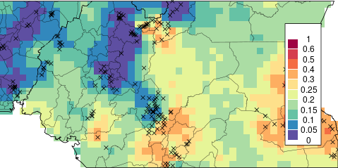
(a) AGHQ

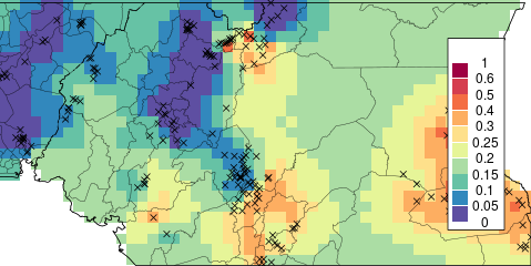
(b) MCMC

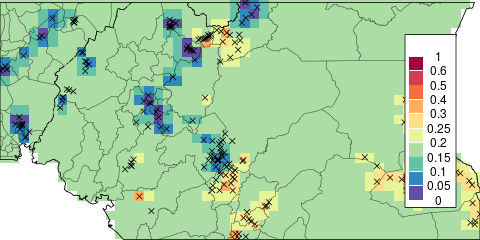
(c) MCML

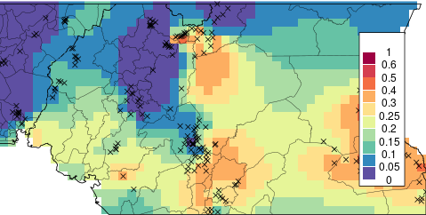
(d) INLA

Figure 5: Spatial interpolations for the four different appraches to inference for the Loa loa example of §4.1.

Method	$\text{mean}|p(\cdot)-p_{\texttt{MCMC}{}}(\cdot)|$	$\text{max}|p(\cdot)-p_{\texttt{MCMC}{}}(\cdot)|$
AGHQ	0.0139	0.101
INLA	0.0304	0.225
MCML	0.0463	0.218

Table 4: Average and maximum discrepancy with MCMC in spatial interpolations for $p(\cdot)$ across the grid on which the maps are drawn, for the three other appraches to inference for the Loa loa example of §4.1.

Method	$2.5\%$	$\hat{\sigma}$	$97.5\%$	$2.5\%$	$\hat{\rho}$	$97.5\%$
MCMC	1.26	1.56	1.97	48.4	68.0	95.8
AGHQ	1.20	1.48	1.81	45.4	63.9	87.5
INLA	1.42	2.06	3.07	93.8	152.	246.
MCML	1.23	1.40	1.60	12.3	15.7	19.9

Table 5: Point and interval estimares of covariance parameters $\sigma$ and $\rho$ (KM) for the four different appraches to inference for the Loa loa example of §4.1.

Method/Task	Fitting	Prediction	Total	Num. Iter
MCMC	465	2055	2520	-
AGHQ	103	92.6	195	465
INLA	-	-	42.7	102
MCML	26.1	10.0	36.2	86.2

Table 6: Runtimes (seconds) and number of MCMC iterations that could have been completed in the same time, for the four different appraches to inference for the Loa loa example of §4.1.

4.2 Zero-inflated Geostatistical Binomial regression: extending the Loa loa model

geostatlowresource describe an extension of the geostatistical binomial regression model which accounts for zero-inflation: the notion that certain spatial locations may be unsuitable for disease transmission and that this may lead to more observed zero counts in the data than would be expected under the binomial model. The likelihood is a discrete mixture of a binomial density and a point mass at zero, and both the transmission and mixing (suitibility) probabilities depend on unknown spatial processes. The resulting model is not a latent Gaussian model and is not compatible with INLA. geostatlowresource fit this challenging model to a different dataset using a frequentist maximum likelihood approach. However, this model is an extended latent Gaussian model, and aghqus fit it using approximate Bayesian inference with AGHQ using the aghq package, making use of its compatibility with TMB. Here we demonstrate the details of the implementation of the zero inflated model using aghq, in the context of extending the non-zero inflated model of §4.1.

Let $\phi(\boldsymbol{s})$ denote the probability that location $\boldsymbol{s}\in\mathbb{R}^{2}$ is suitable for disease transmission. The model is:

$$\mathbb{P}\left(Y_{i}=y_{i}|p(\boldsymbol{s}_{i}),\phi(\boldsymbol{s}_{i})\right) =\left[1-\phi(\boldsymbol{s}_{i})\right]\text{I}\left(y_{i}=0\right)+\phi(\boldsymbol{s}_{i})\times\text{Binomial}[y_{i};N_{i},p(\boldsymbol{s}_{i})],$$ (25)

$$\log\left[\frac{p(\boldsymbol{s})}{1-p(\boldsymbol{s})}\right] =\beta_{\texttt{risk}}+u(\boldsymbol{s}),\ \log\left[\frac{\phi(\boldsymbol{s})}{1-\phi(\boldsymbol{s})}\right]=\beta_{\texttt{zi}}+v(\boldsymbol{s}),\boldsymbol{s}\in\mathbb{R}^{2}$$

$$u(\cdot)|\boldsymbol{\theta} \sim\mathcal{GP}(0,\text{C}_{\boldsymbol{\Xi},u}),\ v(\cdot)|\boldsymbol{\theta}\sim\mathcal{GP}(0,\text{C}_{\boldsymbol{\Xi},v}),$$

where $\left\{Y_{i}|p(\boldsymbol{s}_{i}),\phi(\boldsymbol{s}_{i}):i\in[n]\right\}$ are independent as are $u(\cdot)|\boldsymbol{\theta}$ and $v(\cdot)|\boldsymbol{\theta}$. For simplicity the covariance parameters of the two spatial processes are constrained to be the same.

Making inferences from this model is very challenging due to the two competeing spatial processes, and not easily done using any previously existing packages. To implement this model in aghq, the un-normalized log-posterior $\log\pi(\boldsymbol{W},\boldsymbol{\theta},\boldsymbol{Y})$ is implemented in TMB with the Laplace approximation “turned on” for $\boldsymbol{W}=\left\{u(\boldsymbol{s}_{i}),v(\boldsymbol{s}_{i}),i\in[n];\beta_{\texttt{risk}},\beta_{\texttt{zi}}\right\}$: R> ff <- TMB::MakeADFun(…,random = "W") The template ff has an element ff$fn() which returns $-\log\widetilde{\pi}_{\texttt{LA}}(\boldsymbol{\theta},\boldsymbol{Y})$, including the necessary “inner” optimization of $\log\pi(\boldsymbol{W},\boldsymbol{\theta},\boldsymbol{Y})$ with respect to $\boldsymbol{W}$ (§2.6). Further, an element ff$gr() is provided which computes $-\partial_{\boldsymbol{\theta}}\log\widetilde{\pi}_{\texttt{LA}}(\boldsymbol{\theta},\boldsymbol{Y})$ exactly and—critically—without re-optimizing over $\boldsymbol{W}$. This results in very efficient computations. This template is then passed to aghq::marginal_laplace_tmb(): R> loaloazipquad <- marginal