Bayesian equation selection on sparse data for discovery of stochastic dynamical systems

Abstract

Often the underlying system of differential equations driving a stochastic dynamical system is assumed to be known, with inference conditioned on this assumption. We present a Bayesian framework for discovering this system of differential equations under assumptions that align with real-life scenarios, including the availability of relatively sparse data. Further, we discuss computational strategies that are critical in teasing out the important details about the dynamical system and algorithmic innovations to solve for acute parameter interdependence in the absence of rich data. This gives a complete Bayesian pathway for model identification via a variable selection paradigm and parameter estimation of the corresponding model using only the observed data. We present detailed computations and analysis of the Lorenz-96, Lorenz-63, and the Orstein-Uhlenbeck system using the Bayesian framework we propose.

Keywords: Bayesian variable selection, linchpin MCMC, spike-and-slab priors, Lorenz-63, Lorenz-96.

1 Introduction

In the present era of data-driven scientific discoveries, consequent industrial and commercial applications, and new scientific hypothesis generation, it is useful to understand how experimental and observed data may inform scientists about underlying physical systems. In this paper, we consider data arising from stochastic dynamical systems, and present a detailed and thorough Bayesian route-map of the process of scientific discoveries from noisy data, along with algorithmic innovations that greatly facilitate the computational pathways leading to such discoveries. Along the way, we provide honest discussions on the pitfalls, limitations, and computational challenges of trying to discover “science from data”.

More precisely, we consider a stochastic dynamic system given by

$$d\mathbf{X}_{t}=f(t,\mathbf{X}_{t};\theta)+\Sigma^{1/2}\,d\mathbf{W}_{t}\,,$$ (1)

where $f(\cdot)\in{\mathbb{R}}^{p}$ is the drift function with parameter $\theta$, $\Sigma$ is the $p\times p$ diffusion covariance matrix, and $\mathbf{W}_{t}$ is a standard $p$-dimensional Wiener process. Such dynamical systems are employed in a vast number of natural and social science disciplines, including atmosphere, ocean and other climate and weather systems modeling, systems and control theory, flows and turbulence, molecular dynamics, cancer and other translational biological systems, econometrics and finance, modeling of behavioral and cognitive processes, and so on. For clarity of presentation and precise formulation, in this paper we discuss the Lorenz-96 (Lorenz,, 1996), the Lorenz-63 (Lorenz,, 1963) and the Ornstein-Uhlenbeck (OU) (Uhlenbeck and Ornstein,, 1930) processes in detail. Further, we assume that the continuous process $\{\mathbf{X}_{t}:t\in{\mathbb{R}}\}$ is latent and unobserved, and the observed noisy data is

$$\mathbf{Y}_{i}=\mathbf{X}_{t_{i}}+\epsilon_{i},\,\quad i=1,\ldots,K;$$ (2)

with $\{t_{i}\}_{i=1}^{K}$ being the time-stamps of the associated unobserved latent process $\{\mathbf{X}_{t}\}$. The $\{\epsilon_{i}\}_{i=1}^{K}$ are additive noise in the observed data, which for clarity, we consider to be independent and identically distributed as $p$-dimensional Gaussian random variables with mean zero and known variance $R$. That is, $\epsilon_{i}\overset{\text{iid}}{\sim}\ N_{p}(0,R)$. The $p\times p$ covariance matrix parameter, $R$, is assumed to be known for identifiability. In keeping with real application scenarios, we assume that $K$ is not too large, hence we essentially have sparse data for the scientific modeling process.

In related literature in the physical sciences, the functional form of $f(\cdot)$ is typically assumed known up to a finite number of parameters, and the computational steps and heuristics employed often imply that $\{\mathbf{X}_{t}\}$ is effectively known and fixed, thus resulting in considerably simple computations and underestimation of the uncertainties. Here, we propose a study where neither the drift function nor the latent process is known.

Eliciting the drift function $f(\cdot)$, estimating the unknown parameters: $\theta$ and $\Sigma$, and predicting the unobserved continuous process $\{\mathbf{X}_{t}\}$ are some of the challenges that we address in this paper. Our contributions are threefold: (i) we present a Bayesian variable selection technique for identification and elicitation of the underlying dynamic systems (ii) we discuss the sources of unreliability and instability in inferring dynamical systems from observed data, and (iii) we present computational strategies that are critical in teasing out the important details about the dynamical system from sparse observations. The following example serves as an illustration:

Example: Suppose an atmospheric scientist observes a $p=4$ dimensional time series data, the first component of which is depicted in the left panel of Figure 1. It is surmised that the latent continuous atmospheric diffusion process driving this data has a temporal evolution system that can be reasonably approximated by a low-order polynomial of the state variables. It is possible that the current scientific knowledge informs or conjectures about some terms of this polynomial, or some relations between the polynomial coefficients, and can serve as a starting point for the construction of a digital twin system for the actual stochastic dynamical system.

The Bayesian modeling framework that we propose addresses the above scientific questions using a scheme illustrated on the right panel of Figure 1. The unobserved latent continuous process is denoted by the black curve, the red hollow dots denote a discretized version of the same, and the blue solid dots are the observed data. The goal of this paper is essentially to tease out the equation of the black curve from the blue dots.

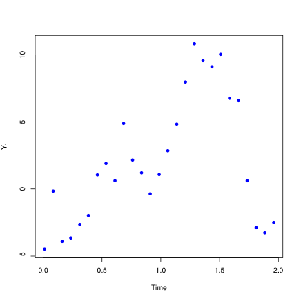
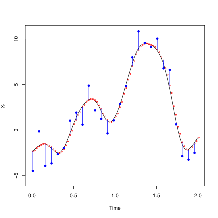
Figure 1: A pictorial representation of the first component of a 4-dimensional Lorenz 96 system. The left panel is the observed data in a time interval $[0,2]$. The right panel contains the same data, but also the latent underlying continuous process (black curve), and it’s discretized version (red dots) over a uniform grid of points.

∎

There are multiple challenges in this process. Notice that the complexity of the problem and sparsity of data are related to the assumed discretization structure (red hollow dots in the right panel of Figure 1) of the continuous latent process $\{\mathbf{X}_{t}\}$ (black curve in the right panel of Figure 1). If we adopt too fine a grid, the discrete representation better captures the properties of the actual latent stochastic process, but leads to a high-dimensional discrete latent variable and considerable computational difficulty, as will be apparent later. A coarse discretization results in a poor representation of the underlying actual stochastic process, and unreliable inference and prediction.

Once a discretization framework is fixed, the first step is to construct a Bayesian variable or model selection framework that allows scientists to choose an appropriate dynamical system from a given dictionary of physically meaningful and interpretable systems. This generally results in selecting an appropriate functional form of the drift function, $f(\cdot)$, from a parametric family of functions. For this, we propose a spike-and-slab prior driven model selection framework. To the best of our knowledge, using Bayesian model selection for eliciting the structure of a dynamical system, or “stochastic ordinary/partial differential equation selection” has not been attempted before.

Once the functional form of $f(\cdot)$ is decided, the estimation of $\theta$ and $\Sigma$, and prediction of $\mathbf{X}$ are the next challenges to address. The posterior distribution of $(\theta,\Sigma,\mathbf{X})$ is particularly complex, because $\mathbf{X}$ is high-dimensional, and because there is high correlation within the $\mathbf{X}$s, as well as large dependency between the $\mathbf{X}$s and $\Sigma$. Also, as noted by Vrettas et al., (2011), the high dependency between the $\mathbf{X}$s and $\Sigma$ yields slow mixing chains in standard Markov chain Monte Carlo (MCMC often hereafter) algorithms. However, we notice that $\Sigma$ can be integrated out of the joint posterior, and this observation leads us to implement a linchpin variable MCMC sampler as described by Archila, (2016). This marginalization yields significant improvements in the mixing of the Markov chain, implying improved quality of estimation.

Current research on studying data from stochastic dynamical systems may be found both in Statistics as well as Physics literature, however, using data in a principled way to discover the underlying stochastic differential equation structure seems new. The existing literature in both Statistics and Physics overwhelmingly use Bayesian methods, but there are important differences. The statistical literature includes theoretical and methodological advances, and may be sampled from Bhaumik and Ghosal, (2014); Brunel et al., (2008); Chkrebtii et al., (2016); Hennig et al., (2015); Lie et al., (2018); Matsuda and Miyatake, (2019); Ramsay et al., (2007); Wang et al., (2020); Zhang et al., (2017) and the numerous papers related to these. While there are important scientific problems studied in these papers, we believe our context involving sparse data and unknown drift function is new, as are the computational advancements that we propose.

A sample of the related literature from the physical sciences may be found in Ala-Luhtala et al., (2015); Apte et al., (2007); Batz et al., (2018); Ching et al., (2006); Pérez-Vieites et al., (2018); Vrettas et al., (2011, 2010). However, we noticed a few possibly significant gaps in statistical treatment in this line of work. Often, to facilitate computations or illustrate the main scientific ideas, ad hoc approximations and assumptions are made, and heuristics are employed. For example, the drift function $f(\cdot)$ may be assumed to be linear or approximated by a linear function. Additionally, the numeric computations may imply that $\{\mathbf{X}_{t}\}$ is effectively fixed and known (and thus neither random nor latent) for the actual Bayesian computation. This is a critical difference, since the uncertainty due to $\{\mathbf{X}_{t}\}$ is not reflected in the estimation or inference steps.

Recently, in order to tackle the high-dimensional nature of the estimation problem, there has been significant work in the use of variational inference algorithms to approximate the posterior distribution. This includes the works of Archambeau et al., (2007); Bauer et al., (2017); Yu et al., (2018) and many others. As we will demonstrate, in many chaotic systems, a small deviation away from the underlying true parameters can have dramatic effects on inference for such models. Thus, approximations to the true posterior distribution with no quantification of the approximation error (as is the case with variational Bayes algorithms), can lead to dramatically unreliable inference.

In a different direction, Eraker, (2001) propose a component-wise MCMC algorithm for discretized univariate diffusions. However, the high dependence between the $\mathbf{X}$s yields large auto-correlation and high cross-correlation in the Markov chain. When the functional form $f(\cdot)$ is known but involves many parameters with adequate available data, and a Euler-Maruyama approximation is not required for the statistical model, the approach due to Zhang et al., (2017) may be used.

In Section 2 below, we present in detail the spike-and-slab model that we adopt in this paper. Our proposed Bayesian algorithm and the computational aspects are described in Section 3. In Section 4, we analyze the performance of our proposed dynamic stochastic model selection paradigm and subsequent inference for data obtained by three systems: a Lorenz 96, an Ornstein-Uhlenbeck process, and a particularly chaotic Lorenz 63 model. In all three examples, our model is successfully able to identify the underlying dynamical process. We also draw attention to the performance of MCMC when reasonable starting values of the latent paths is unavailable and caution practitioners against short MCMC runs often witnessed in the literature. Our conclusions are summarized in Section 5. Additional technical details are included in the supplementary materials.

2 Spike-and-slab model for system identification

Recall that $t_{1}$ and $t_{K}$ are the time-stamps for the first and last observations. We first use an Euler-Maruyama discretization step on $\{\mathbf{X}_{t}\}$, to obtain the latent vector $\mathbf{X}=(\mathbf{X}_{0},\dots,\mathbf{X}_{N})$, where we select a grid-size $\delta t$ and define $N=(t_{K}-t_{1})/\delta t$. The discrete latent vector ($\mathbf{X}$) and the continuous latent process ($\{\mathbf{X}_{t}\}$) have similar but distinct notations, to signify their close correspondence. Based on (1), this discretization yields the Markovian structure

$$\mathbf{X}_{k+1}=\mathbf{X}_{k}+f(t,\,\mathbf{X}_{k};\theta)\delta t+\sqrt{\Sigma\delta t}\,\xi_{k}\,,$$

where $\xi_{k}\sim N_{p}(0,I_{p})$ for $k=0,\dots,N-1$. Thus, the joint density of $\mathbf{X}$ satisfies

$$\pi(\mathbf{X})=\pi(\mathbf{X}_{0})\,\prod_{i=1}^{N}\pi(\mathbf{X}_{i}|\mathbf{X}_{i-1})\,,$$

where $\pi(\mathbf{X}_{i}|\mathbf{X}_{i-1})$ is the density of $N_{p}(\mathbf{X}_{i-1}+f(t,\mathbf{X}_{i-1};\theta),\Sigma\delta t)$ distribution.

As an illustrative framework for the spike-and-slab equation selection process, suppose we have a first order (stochastic) differential equation as in (1), where the drift function is a sparse quadratic function of the state variables and time. Define $\tilde{\mathbf{X}}$ to be the vector containing linear, quadratic, and cross terms of the system components of $\mathbf{X}$, along with linear and quadratic time components, $t$ and $t^{2}$ appended at the end. Therefore, this vector contains all possible combination of terms up to order 2 that can occur in a dynamic system.

Let $\tilde{\mathbf{X}}$ then be $p^{*}$ dimensional and let $B(t,\theta)$ be a $p\times p^{*}$ matrix so that the drift function for a desired stochastic differential equation can be written as

$$f(t,\mathbf{X}_{k},\theta)=B(t,\theta)\tilde{\mathbf{X}}_{k}\,.$$

For convenience, we use the notation $B(t,\theta)=B$. Then, the modified system equation for this generic drift function is

$$\dfrac{d\mathbf{X}}{dt}=B\,\tilde{\mathbf{X}}+\Sigma^{1/2}\,dW_{t}\,,$$ (3)

with the corresponding Euler-Maruyama discretization being

$$\mathbf{X}_{k+1}=\mathbf{X}_{k}+B\,\tilde{\mathbf{X}}_{k}\delta t+\sqrt{\Sigma\delta t}\,\xi_{k}\,.$$

In realistic systems, we expect many entries of $B$ to be zero, and consequently many terms in $\tilde{\mathbf{X}}$ may not appear in the drift function.

As an example, consider the four-dimensional stochastic Lorenz 96 model with the drift function described in Lorenz, (1996). Here $\mathbf{X}_{t}=({X_{t}^{1}},\dots,{X_{t}^{4}})$ and

$$dX_{t}^{i}=[(X_{t}^{i+1}-X_{t}^{i-2})\,X_{t}^{i-1}-X_{t}^{i}+\theta]\,dt+\Sigma_{i}^{1/2}\,dW_{t}^{i}\,,$$

where $i\in\{1,2,3,4\}$ are cyclic indices and $\theta\in\mathbb{R}$ is the drift parameter. The drift equations here are often used to represent a simplified atmospheric model (see for example Lorenz and Emanuel,, 1998). For this system, $\tilde{\mathbf{X}}$ is

$$[1,X^{1},X^{2},X^{3},X^{4},{X^{1}}^{2},{X^{2}}^{2},{X^{3}}^{2},{X^{4}}^{2},{X^{1}}X^{2},X^{1}X^{3},X^{1}X^{4},X^{2}X^{3},X^{2}X^{4},X^{3}X^{4},t,t^{2}]^{T}\,.$$

The corresponding $B$ matrix in (3) is all 0s, except for non-zero elements in indices (column-wise) $(1,2,3,4,5,10,15,20,39,42,44,46,52,53,55,57)$ with the first four being $\theta$ and the others being either -1 or 1 appropriately.

This illustrative framework can be easily extended to more complex dynamical systems, including those that potentially involve higher order derivative with respect to time and space variables, higher order polynomials in state, location and time variables, and transformations of such variables.

Continuing with the above illustrative framework, we employ a spike-and-slab prior on the elements of the matrix $B$ to identify the components of $\tilde{\mathbf{X}}$ which have a significant impact on the system underlying the observed data. Our prior choice is based on the works of George and McCulloch, (1993); Ishwaran et al., (2005); Narisetty and He, (2014). Each component of $B$ is given an independent hierarchical prior as:

$$B_{i,j}|\gamma_{i,j} \overset{\text{ind}}{\sim}(1-\gamma_{i,j})N(0,\tau_{0}^{2})+\gamma_{i,j}N(0,\tau_{1}^{2})$$ (4)

$$\gamma_{i,j} \overset{\text{ind}}{\sim}\text{Bernoulli}(q_{i,j})\,,$$ (5)

where $\tau_{0}>0$ is small and $\tau_{1}$ is at least an order of magnitude larger than $\tau_{0}$. Therefore, if $\gamma_{i,j}=0$, the value of $B_{i,j}$ is confined to a narrow region around 0, nullifying its contribution in the model equation. Additional scientific prior knowledge about the parameters $B_{i,j}$’s can be easily absorbed in the $q_{i,j}$’s.

Additionally, we assume a Gaussian prior on $\mathbf{X}_{0}$ as well so that $\mathbf{X}_{0}\sim N_{p}(\mu_{0},\lambda_{0}^{2})$. We assume that $\Sigma$ is a diagonal matrix with $\Sigma_{i}\overset{\text{iid}}{\sim}\text{Inverse-Gamma}(\alpha,\beta)$ for $i=1,\dots,p$. Suppose $\theta=(\theta_{1},\dots,\theta_{d})\in\mathbb{R}^{d}$ contains the $d$ drift parameters. The prior on $\theta$ is

$$\theta \sim N_{d}(m_{0},s^{2}_{0}I_{d})\,,$$

where $s^{2}_{0}$ and $m_{0}$ are hyper-parameters. The resulting posterior distribution of $(\theta,\Sigma,\mathbf{X})$ is presented in the supplementary materials. An MCMC sampler described in Section 3 yields posterior probabilities of association for each $\gamma_{i,j}$. A median cutoff of $0.5$ (Ročková and George,, 2018) on the posterior probabilities of association is employed to determine whether a component is to be deemed active or inactive.

Once a list of final important components is determined by the above process and a reduced stochastic differential equation structure identified using the above process, we propose a second round of computation using only the reduced equation system to obtain posterior distributions of the finite dimensional parameters. We are fully aware of the theoretical and statistical difficulties arising from such two-stage computations, and the super-efficient nature of the estimation and inference obtained from the second round of computations. While caution about superefficiency is valid, the reason for our advocacy of a two-stage computational process is more practical: the initial model in (3) may be very high-dimensional and the posterior distributions of the true (non-zero) parameters too imprecise for scientific use, especially considering the fact that we have limited and sparse data at hand. We use the term inference model for the reduced system discovered by the above Bayesian equation selection process.

3 Posterior Computation

The posterior density for the spike-and-slab model is given by

$$\pi(\mathbf{X},B,\Sigma,\gamma\mid\mathbf{Y}) \propto\pi(\mathbf{Y}\mid\mathbf{X},B)\,\pi(\mathbf{X}\mid B,\Sigma)\,\pi(B\mid\gamma)\,\pi(\Sigma)\,,$$

and is naturally intractable, with MCMC methods being used to obtain posterior estimates. There are some obvious challenges here. First, the overall dimension of $\mathbf{X}$ is typically quite large since $\delta t$ is usually small. In addition, there is high correlation across time in the $\mathbf{X}$s, implying that component-wise updates on the $\mathbf{X}$s would lead to debilitating performance. Thus, we will focus on full block updates for the $\mathbf{X}$s.

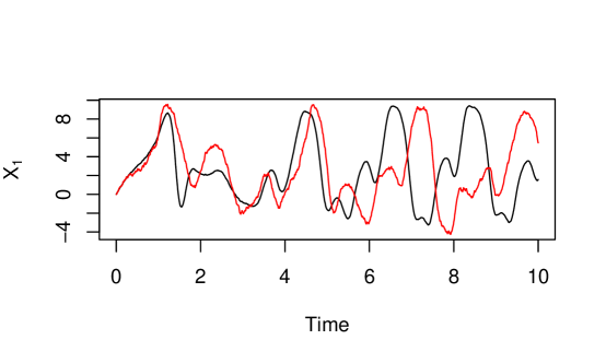
Figure 2: Two realizations of the first component of Lorenz 96 with $\Sigma_{1}=.05$ (black) and $\Sigma_{1}=1$ (red).

There is a particularly delicate relationship between $\Sigma$ and $\mathbf{X}$. Small changes in $\Sigma$ leads to a butterfly effect in the trajectory of the system. Consider Figure 2 where we present two trajectories of the first component of a Lorenz 96 system with two different values of $\Sigma$ over 10 time units. In the beginning, the two processes behave similarly, but with time the difference in the trajectories is exaggerated. This implies that small shifts in the estimation of the $\mathbf{X}$s yield large deviations in the $\Sigma$s and vice-versa. Additionally, this subtle balance restricts the movement of any Markov chain, encouraging tiny steps and weak exploration. This was also noticed in the Hamiltonian Monte Carlo algorithm implemented in Vrettas et al., (2011).

We construct a linchpin sampler presented in Archila, (2016) where we integrate out $\Sigma$ and run an MCMC kernel that keeps the marginal posterior of $\pi(\mathbf{X},B,\gamma|\mathbf{Y})$ stationary. The draws from this marginal are then cycled through to the full conditional distribution of $\Sigma$, allowing its estimation as well. Notice that,

$$\pi(\mathbf{X},B,\Sigma,\gamma\mid\mathbf{Y})=\pi(\Sigma\mid\mathbf{X},B,\gamma,\mathbf{Y})\,\pi(\mathbf{X},B,\gamma\mid\mathbf{Y})\,,$$

with each diagonal $i$ of $\Sigma$ having the full conditional,

$$\Sigma_{i}|\mathbf{X},B,\gamma,\mathbf{Y}\sim\text{inv-gamma}\left(\dfrac{N}{2}+\alpha,\,\beta+\dfrac{\delta t}{2}\,\sum_{j=0}^{N-1}\left(\dfrac{\delta\mathbf{X}_{j+1}}{\delta t}-B\tilde{\mathbf{X}}_{j}\right)^{2}_{i}\right)\,,$$ (6)

where $(\cdot)_{i}$ represents the $i$th element of the vector. The full conditional of each $\gamma$ is

$$P(\gamma_{i,j}=1|\textbf{X},\theta,\textbf{Y})=\dfrac{\left(\dfrac{q_{i,j}}{\sqrt{2\pi\tau_{1}^{2}}}\exp\left(-\dfrac{B_{i,j}^{2}}{2\tau_{1}^{2}}\right)\right)}{\dfrac{q_{i,j}}{\sqrt{2\pi\tau_{1}^{2}}}\exp\left(-\dfrac{B_{i,j}^{2}}{2\tau_{1}^{2}}\right)+\dfrac{1-q_{i,j}}{\sqrt{2\pi\tau_{0}^{2}}}\exp\left(-\dfrac{B_{i,j}^{2}}{2\tau_{0}^{2}}\right)}\,.$$ (7)

Exact calculations and expressions can be found in the supplementary materials. Since the marginal posterior distribution of $(\mathbf{X},B,\gamma)$ demonstrates significantly less correlation in its components, the linchpin sampler moves with considerable freedom and mixes much faster.

For updating $(\mathbf{X},B,\gamma)$, we employ a component-wise MCMC algorithm with random-walk Metropolis-Hastings (MH) updates for $\mathbf{X}$ and each element of $B$ and a Gibbs update on $\gamma$. Thus the number of components in the MCMC update are $2pp^{*}+1$. Before zeroing in on the random-walk MH update, we tested the Hamiltonian Monte Carlo and the No-U-Turn-Samplers. Since the posterior distribution, particularly for the $\mathbf{X}$s lies in a narrow region, we found that both algorithms via their implementation in Stan, struggled to either reach or stay in this region. In addition, the leapfrog integrator required a large number of steps, leading to an implementation that was significantly slower than the random-walk MH updates available in the R package mcmc (Geyer and Johnson,, 2020). Similar struggles are witnessed in the random-walk MH update for $\mathbf{X}$ as well, however, with some careful tuning of the scaling, the random-walk MH significantly improves the mixing in the sampler.

For the inference model (i.e., the model obtained by the Bayesian equation selection process of the previous section), a similar linchpin sampler is possible where

$$\pi(\mathbf{X},\theta,\Sigma|\mathbf{Y})=\pi(\Sigma|\mathbf{X},\theta,\mathbf{Y})\,\pi(\mathbf{X},\theta|\mathbf{Y})\,,$$

with each diagonal $i$ of $\Sigma$ having the full conditional

$$\Sigma_{i}|\mathbf{X},\theta,\mathbf{Y}\sim\text{inv-gamma}\left(\dfrac{N}{2}+\alpha,\,\beta+\dfrac{\delta t}{2}\,\sum_{j=0}^{N-1}\left(\dfrac{\delta\mathbf{X}_{j+1}}{\delta t}-f(t,\mathbf{X}_{j},\theta)\right)^{2}_{i}\right)\,.$$ (8)

The MCMC algorithm employed for the marginal posterior of $(\mathbf{X},\theta)$ is a random-walk MH with scaling chosen to obtain around 23% acceptance, as recommended by Roberts et al., (1997).

The slow mixing of the Markov chains in such high-dimensions brings a critical challenge of choosing starting values for the Markov chain. Since $\Sigma$ is integrated out, starting values of $\Sigma$ are not required. However, choosing starting values of the $\mathbf{X}$s is particularly challenging. The joint posterior distribution of the $\mathbf{X}$s takes mass in a narrow region, from where it is close to impossible to start the Markov chain unless the true latent process is known. As also discussed in Sørensen, (2004), a reasonable starting value is to interpolate the observed $\mathbf{Y}$s, which is what we employ here. Due to the narrow high probability region, one cannot afford to make large jumps for the $\mathbf{X}$s, implying slow converge of the latent process. Naturally, this in turn also affects the $\Sigma$s. However, we note that, in general, the drift parameters, $\theta$ do not contribute significantly to the slow mixing rate.

4 Examples

We implement our proposed spike-and-slab model for system identification for data generated from three systems: (i) Lorenz 96 (L96) (ii) Ornstein-Uhlenbeck system (OU) (iii) Lorenz 63 (L63). The data generation settings for each system are in Table 1. For the hyper-parameter settings for this model, we use the rule of Narisetty and He, (2014) multiplied by an appropriate scaling factor so that $\tau_{0}$ and $\tau_{1}$ lie in the range $(0,1)$ and $(2,10)$, respectively. These values ensure that there is adequate separation between the spike and slab components to deter random jumping of $\gamma$ values while allowing for easy switching in $\gamma$ if the model finds corresponding components to be significant (or insignificant).

Table 1: Parameter settings for the examples. Additionally, $\delta t=.01$, $N_{\text{obs}}=20$ and $R=.05$ for all systems.

System	$t_{K}$	$\theta$	$\Sigma$	burn-in	# parameters	$\tau_{0}$	$\tau_{1}$
L96	10	8	0.5	50	4,009	0.13	4.52
L63	20	(10, 28, 8/3)	0.6	5000	6,009	0.50	5.00
OU	2	2	1.0	50	203	0.09	2.90

Practitioners typically have prior information about which system may best align with their data. Thus, we set $q_{i,j}=.90$ for the elements of $B$ which are deemed active under this prior knowledge and set $q_{i,j}=.10$ for elements of $B$ which are deemed inactive. Once a system is identified, we then run the Bayesian inferential model to obtain posterior estimates of $\theta$, $\Sigma$, and $\mathbf{X}$.

4.1 Lorenz 96

Recall the four-dimensional stochastic Lorenz 96 model introduced in Section 2:

$$dX_{t}^{i}=[(X_{t}^{i+1}-X_{t}^{i-2})\,X_{t}^{i-1}-X_{t}^{i}+\theta]\,dt+\Sigma_{i}^{1/2}\,dW_{t}^{i}\,,$$

where $i\in\{1,2,3,4\}$ are cyclic indices and $\theta\in\mathbb{R}$ is the drift parameter.

For generating a Lorenz-96 trajectory using Euler-Maruyama approximation, we use $\delta t=0.01$ for the time interval $T=[0,10]$ with the true value of the parameter as $\theta=8$. We have an additional burn-in of $T=50$ time units to allow the process to reach a level of stationarity. Due to the Euler-Maruyama discretization, $N=1000$ values are generated after this initial burn-in. We observe 20 data points per time unit, so that overall $K=200$. This takes the total number of estimated parameters ($\textbf{X},\theta$) and the diagonal elements of $\Sigma$) to $4,009$ ($4\times 1001+1+4$). The true diagonal covariance matrix $\Sigma$ is $0.5\,I_{4}$ and we fix $R=0.05\,I_{4}$.

First, we perform model identification for Lorenz-96 using our proposed spike-and-slab model. We run the linchpin samplers initialized both at the truth and with interpolated values of $\mathbf{X}$ for Monte Carlo sample sizes 50000 and $10^{5}$, respectively. We mention here that longer Markov chain lengths do not impact the inference on the $\gamma$s, thus we limit the MCMC to shorter runs for this step. In Figure 3, we present posterior mean estimates of the $\gamma$s, color coded with what their value should be under the Lorenz-96 model. Red implies active, and black implies inactive. We find that the quality of inference is the same for both runs and the Lorenz 96 system is correctly identified.

Having identified the Lorenz-96 model, we run the inference model for $10^{6}$ steps using the Lorenz-96 drift function in order to estimate parameter, $\theta$, and infer the $\Sigma$s. We set $m_{0}$ to be centered at the estimate of the parameter from the spike-and-slab estimates, in order to allow some reasonable centering in the prior information for this chaotic system.

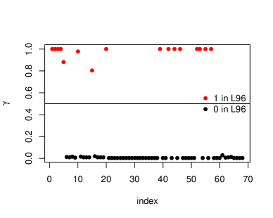
Figure 3: Posterior mean estimates of $\gamma$ for each element of $B$ for Lorenz 96, with X initialized at its truth (left) and interpolated starting values (right).

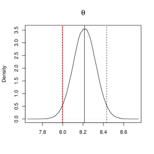
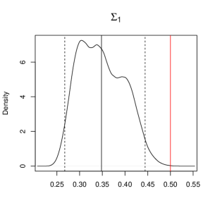
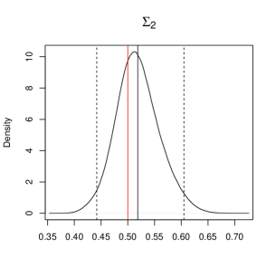
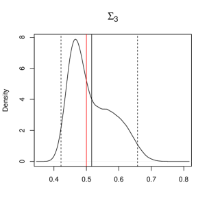
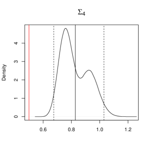
Figure 6: Posterior density estimates of $\theta$ and the diagonals of $\Sigma$ for Lorenz 96. Results are for interpolated $\mathbf{X}$ as starting values.

We present results for the run from the interpolated starting point of the $\mathbf{X}$s. Due to the slow mixing of the inferential model, we ran the Markov chain for 5 million steps and noticed that for the first 4 million, the Markov chain demonstrated a lack of stationarity and a significant drift in the estimates of $\Sigma$. Thus only the last 1 million steps are used for estimation and their posterior density estimates are presented in Figure 6. It is clear that the parameter $\theta$ is well estimated. However, as is expected from the vulnerable relationship between the $\mathbf{X}$s and $\Sigma$, the $\Sigma$s are reasonably estimated, although some discrepancy remains due to lack of information on the true $\mathbf{X}$s.

A comparison of the linchpin sampler and vanilla MH on $(\theta,\Sigma,\mathbf{X})$ shows that the Markov chain for the former displays significant improvements over vanilla MH. Figure 4 shows the ACF for the drift parameter plots of the two samplers, with correlation in the chain decaying at a faster rate for linchpin sampler than vanilla MH. Additionally, the effective sample size (calculated using R package mcmcse (Flegal et al.,, 2020)) for $\theta$ for the two samplers is $12697$ and $2688$ for a $10^{5}$ length run, respectively, indicating the superiority in performance of our linchpin sampler.

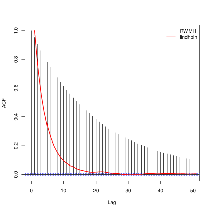
Figure 4: Autocorrelation of vanilla MH vs linchpin sampler for the inference model.

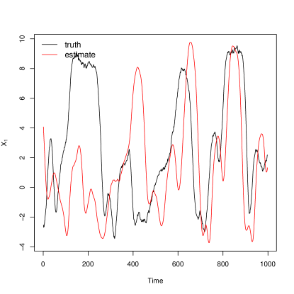
Figure 5: Truth vs posterior mean trajectories of the first component of Lorenz-96.

4.2 Ornstein-Uhlenbeck

The Ornstein–Uhlenbeck (OU) is a univariate process defined by the following SDE

$$dx_{t}=-\theta x_{t}dt+\Sigma dW_{t}\,,$$

where $\theta\in\mathbb{R}$ is the drift parameter. The OU trajectory is generated for the time interval $T=[0,2]$ with the drift parameter $\theta=2$ using the Euler-Maruyama approximation with $\delta t=0.01$ discretization steps. Similar to Lorenz-96, we have a burn-in of $T=50$ time units for the EM approximation for the model to reach stationarity. The total number of parameters to be estimated ($\textbf{X},\theta$ and $\Sigma$) are $203$ ($201+1+1$), with $K=40$ observations. The observation error is fixed at $R=0.05$, and we use $\Sigma=1$ to generate the process.

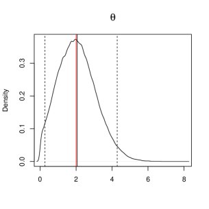
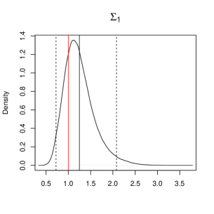
Figure 7: OU estimated marginal posterior densities. Results are for interpolated $\mathbf{X}$ as starting values.

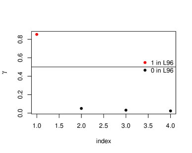
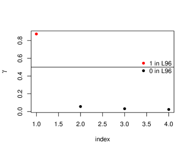
Figure 8: Posterior mean estimates of $\gamma$ for OU, with X initialized at its truth (left) and interpolation (right).

We first perform model identification for the OU system using samplers initialized at the truth and at interpolations from Y, using run lengths of $50000$ and $10^{5}$ respectively. The results from our spike-and-slab model in Figure 8 show that the OU system is correctly identified. Next, we run the linchpin based inference model for $10^{6}$ steps with the OU drift function for X initialized at values interpolated from Y. Similar to Lorenz-96, we set $m_{0}$ as the estimate of the parameter from the spike-and-slab model. Figure 7 shows that $\theta$ and $\Sigma$ are estimated well. Since OU had only $200$ latent variables to estimate, compared to $4004$ for Lorenz-96, the sampler has a much easier job in estimation, the effect of which is translated into better quality estimates of $\theta$ and $\Sigma$.

4.3 Lorenz-63

The stochastic Lorenz-63 is driven by the following SDE:

$$d\mathbf{X}_{t} =\begin{bmatrix}\sigma\left(y_{t}-x_{t}\right)\\ \rho x_{t}-y_{t}-x_{t}z_{t}\\ x_{t}y_{t}-\beta z_{t}\end{bmatrix}dt+\Sigma^{1/2}d\textbf{W}_{t}\,,$$ (9)

where $(\sigma,\rho,\beta)\in\mathbb{R}^{3}$ are the drift parameters.

We use Euler-Maruyama approximation with $\delta t=0.01$ discretization to generate Lorenz-63 trajectory for the time interval $T=[0,20]$. We use parameters $\theta=[\sigma,\rho,\beta]=[10,28,8/3]$ since this choice exhibits chaotic behavior. Similar to the previous two examples, an additional burn-in of $T=5000$ time units for the EM approximation allow the chaotic model to reach stationarity. We generate $N=2000$ values after the burn-in, taking the total number of estimated parameters ($\textbf{X},\theta$ and the diagonal elements of $\Sigma$) to $6,009$ ($3\times 2001+3+3$). The diagonal covariance matrix $\Sigma$ is $0.6\,I_{3}$ and the covariance matrix of the observation matrix $R=0.05\,I_{3}$. We observe $20$ values of X per time unit with added measurement error, giving a total of $K=400$ real observations Y.

The spike-and-slab model for model identification of Lorenz-63 correctly captures the chaotic system for samplers initializing X from the truth as well as interpolation with run lengths of $50000$ and $10^{5}$ respectively (see Figure 9). Having identified the system as Lorenz-63, we move on the estimation of parameters and latent variables using the linchpin inference model. Similar to the previous two examples, we set the prior mean $m_{0}$ to be the parameter estimates from the spike-and-slab model to encapsulate prior knowledge about the system and run the sampler for $10^{6}$ steps. Note that Lorenz-63 is an extremely chaotic system in which slight variations in the drift parameters or $\Sigma$ significantly modify the system trajectory. The parameter estimates for the sampler with X initialized at interpolations are $(9.9,27.9,2.66)$ which is very close to the true value of $(10,28,2.67)$. Despite this proximity, the L63 trajectory formed by using the estimates as the drift parameters differs significantly from the original trajectory (see Figure 10).

The inference results of $\Sigma$ for the inference run in Figure 11 mirror the difficulty in estimating X given their chaotic nature and high-dimensionality. To understand the dependence of estimates of $\Sigma$ on X, we add Gaussian noise to the Euler-Maruyama approximation of the $\mathbf{X}$ with $\theta=(10,28,8/3)$ and $\Sigma=0.06$. We use these values to calculate the mean of the posterior conditional of $\Sigma$ (Equation 8). The trajectories of X with added noise overlapped with the EM approximation in Figure 12 and corresponding conditional posterior means in Table 2 show that even minor variations in $\mathbf{X}$s offsets $\Sigma$ by orders of magnitude in the Lorenz-63 system. In spite of the complications introduced by the relationship between X and $\Sigma$, the drift parameters $\theta=[\sigma,\rho,\beta]$ are estimated fairly well owing to the decoupling by the linchpin posterior decomposition.

5 Future work

In this paper, we assume that the variance of the noise in the observed data, $R$ is known. While this is in keeping with assumptions made in the literature (Vrettas et al.,, 2011) and a requirement for identifiability, it can be circumvented if additional observations can be taken, for example, if multiple realizations of $Y_{i}$ can be observed at each $i=1,\ldots,K$.

Replacing the continuous time stochastic process $\{\mathbf{X}_{t}\}$ with the vector $\mathbf{X}$ using the Euler-Maruyama discretization process induces errors in the numeric computations. There are several techniques to address this issue, for example, see Beskos et al., (2008, 2009); Chkrebtii et al., (2016); Hennig et al., (2015); Lie et al., (2018); Matsuda and Miyatake, (2019); Wang et al., (2020) and references therein. The sparsity of data may render some of the alternative techniques from the literature unavailable in the current context. An alternative may be to use a functional representation of the data, as in Bhaumik and Ghosal, (2014); Brunel et al., (2008); Ramsay et al., (2007); Zhang et al., (2017) and in several other sources. We will explore this option in future, but anticipate complications due to the chaotic nature and nonlinear lagged structure of the Lorenz-96 and Lorenz-63 systems. It has been noted earlier in Vrettas et al., (2011) that a large number of basis functions are often needed to capture the roughness of the observed physical data. Variational algorithms are favored in the related physical sciences literature, and while these have serious shortcomings, they may be useful for obtaining some quantifiers (for example, location parameters) of the posterior distribution relatively quickly, which may help in the actual MCMC computations.

We have adopted a spike-and-slab prior in this paper. Naturally, other Bayesian sparse system modeling frameworks, for example using the horseshoe prior, may also be explored and studied in this context. The statistical theory related to the methodologies presented here is non-trivial because of the multi-stage computational technique we adopt, and will be developed in a future publication.

Acknowledgments: (to be filled in for an accepted manuscript).

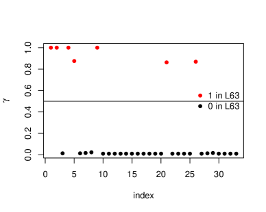
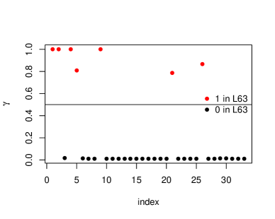
Figure 9: Posterior mean estimates of $\gamma$ for Lorenz 63, with $\mathbf{X}$ initialized at its truth (left) and with $\mathbf{X}$ initialized at interpolation.

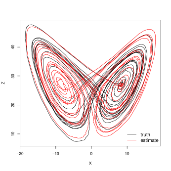
Figure 10: Lorenz-63 trajectory from the truth $(10,28,2.67)$ and estimates $(9.9,27.9,2.66)$.

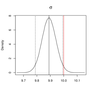
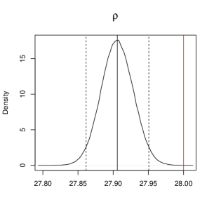
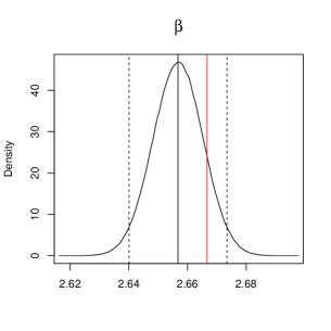
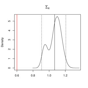
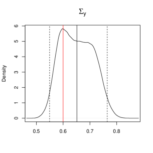
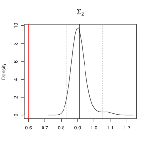
Figure 11: Lorenz 63 parameter density, starting X at interpolation.

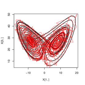
(a) sd = 1

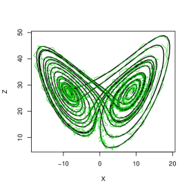
(b) sd = 0.5

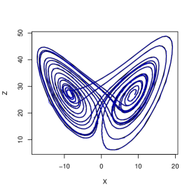
(c) sd = 0.1

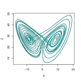
(d) sd = 0.05

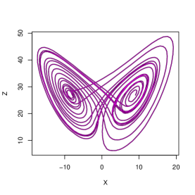
(e) sd = 0.01

Figure 12: Lorenz-63 trajectory with Gaussian noise

Table 2: Mean of posterior conditional of $\Sigma$ for Lorenz 63 with N(0,$s^{2}$) noise added to X. The true value of $\Sigma$ for the underlying trajectory is $0.06$.

Noise variance	$s=1$	$s=0.5$	$s=0.1$	$s=0.05$	$s=0.01$
$\Sigma_{x}$	185.1	44.2	2.03	0.53	0.086
$\Sigma_{y}$	198.9	48.7	2.02	0.54	0.084
$\Sigma_{z}$	206.8	47.3	2.04	0.52	0.084

Appendix A Prior and Posterior Calculation

Define $\Theta=(\theta,\Sigma)$ where $\theta\in\mathbb{R}^{d}$ are the parameters of the process and $\Sigma\in\mathbb{R}^{p}\times\mathbb{R}^{p}$ is the diffusion covariance matrix. Using a $N(\mu_{0},\lambda^{2}_{0})$ prior on the first component of X (i.e. $\mathbf{X}_{0}$), the priors for the latent variables $\mathbf{X}$ using the Euler-Maruyama approximation can be written as:

$$P(\mathbf{X}_{0:N}\mid\Theta)$$

$$=P(\mathbf{X}_{0})\prod_{i=1}^{N}P(\mathbf{X}_{i}\mid\mathbf{X}_{i-1})$$

$$=P(\mathbf{X}_{0})\prod_{i=1}^{N}\mathbf{N}\left(\mathbf{X}_{i}\mid\mathbf{X}_{i-1}+f(t,\mathbf{X}_{i-1}))\delta t\,,\Sigma\delta t\right)$$

$$=P(\mathbf{X}_{0})\prod_{i=0}^{N-1}(2\pi)^{-p/2}|\Sigma\delta t|^{-1/2}\exp\left\{-0.5\left(\mathbf{X}_{i+1}-\mathbf{X}_{i}-f(t,\mathbf{X}_{i},\theta)\delta t\right)^{T}\left(\Sigma\delta t\right)^{-1}\right.$$

$$\qquad\qquad\left(\mathbf{X}_{i+1}-\mathbf{X}_{i}-f(t,\mathbf{X}_{i},\theta)\delta t\right)\bigg{\}}$$

$$=P(\mathbf{X}_{0})(2\pi)^{-\frac{Np}{2}}|\Sigma\delta t|^{-\frac{N}{2}}\exp\left[\dfrac{-\delta t}{2}\sum_{i=0}^{N-1}\left(\dfrac{\delta\mathbf{X}_{i+1}}{\delta t}-f(t,\mathbf{X}_{i},\theta)\right)^{T}\Sigma^{-1}\left(\dfrac{\delta\mathbf{X}_{i+1}}{\delta t}-f(t,\mathbf{X}_{i},\theta)\right)\right]$$

$$=(2\pi)^{-p/2}|\lambda_{0}^{2}|^{-1/2}\exp\left\{-0.5(\mathbf{X}_{0}-\mu_{0})^{T}(\lambda_{0}^{2})^{-1}(\mathbf{X}_{0}-\mu_{0})\right\}(2\pi)^{-Np/2}|\Sigma\delta t|^{-N/2}$$

$$\quad\quad\exp\left[-\dfrac{\delta t}{2}\sum_{i=0}^{N-1}\left(\dfrac{\delta\mathbf{X}_{i+1}}{\delta t}-f(t,\mathbf{X}_{i},\theta)\right)^{T}\Sigma^{-1}\left(\dfrac{\delta\mathbf{X}_{i+1}}{\delta t}-f(t,\mathbf{X}_{i},\theta)\right)\right]\,.$$

For the $d$ elements of $\theta$, the priors are independent $N(m_{0,j},s_{0}^{2})$ for $j\in{1,2...,d}$ and the priors for the diagonal elements of $\Sigma$ are i.i.d inverse-gamma($\alpha,\beta)$ .
The likelihood of the model is given by

$$P(\mathbf{Y}|\mathbf{X},\theta,\Sigma) =\prod_{i=1}^{K}P(\mathbf{Y}_{i}|\mathbf{X}_{t_{i}},\theta,\Sigma)$$

$$=\prod_{i=1}^{K}(2\pi)^{-p/2}|R|^{-1/2}\,\exp\left(-\dfrac{(\mathbf{Y}_{i}-\mathbf{X}_{t_{i}})^{T}R^{-1}(\mathbf{Y}_{i}-\mathbf{X}_{t_{i}})}{2}\right)$$

$$=(2\pi)^{-Kp/2}|R|^{-K/2}\exp\left(-\sum_{i=1}^{K}\dfrac{(\mathbf{Y}_{i}-\mathbf{X}_{t_{i}})^{T}R^{-1}(\mathbf{Y}_{i}-\mathbf{X}_{t_{i}})}{2}\right)\,.$$

Therefore, the final form of the posterior can be written as

$$P\left(\mathbf{X},\Theta|\mathbf{Y}\right)$$

$$\propto P(\mathbf{Y}|\mathbf{X},\theta,\Sigma)\,P(\mathbf{X})\,P(\Sigma)\,P(\theta)$$

$$\propto(2\pi)^{-Kp/2}|R|^{-K/2}\exp\left[-0.5\sum_{i=1}^{K}(\mathbf{Y}_{i}-\mathbf{X}_{t_{i}})^{T}R^{-1}(\mathbf{Y}_{i}-\mathbf{X}_{t_{i}})\right](2\pi)^{-p/2}|\lambda_{0}^{2}|^{-1/2}$$

$$\quad\quad\times\exp\left[-0.5(\mathbf{X}_{0}-\mu_{0})^{T}(\lambda_{0}^{2})^{-1}(\mathbf{X}_{0}-\mu_{0})\right](2\pi)^{-Np/2}|\Sigma\delta t|^{-N/2}$$

$$\quad\quad\times\exp\left[-\dfrac{\delta t}{2}\sum_{i=0}^{N-1}\left(\dfrac{\delta\mathbf{X}_{i+1}}{\delta t}-f(t,\mathbf{X}_{i},\theta)\right)^{T}\Sigma^{-1}\left(\dfrac{\delta\mathbf{X}_{i+1}}{\delta t}-f(t,\mathbf{X}_{i},\theta)\right)\right]$$

$$\quad\quad\times\prod_{i=1}^{d}\left[\exp\left(-\dfrac{(\theta_{i}-m_{0,i})^{2}}{2s^{2}_{0}}\right)\right]\,\prod_{i=1}^{p}\left[\dfrac{\beta^{\alpha}}{\Gamma(\alpha)}\Sigma_{i}^{-\alpha-1}\exp\left(-\dfrac{\beta}{\Sigma_{i}}\right)\right]$$

$$\propto\exp\left[-0.5\left(\sum_{i=1}^{K}(\mathbf{Y}_{i}-\mathbf{X}_{t_{i}})^{T}R^{-1}(\mathbf{Y}_{i}-\mathbf{X}_{t_{i}})+(\mathbf{X}_{0}-\mu_{0})^{T}(\lambda_{0}^{2})^{-1}(\mathbf{X}_{0}-\mu_{0})\right.\right.$$

$$\quad\quad+\left.\left.\delta t\sum_{i=0}^{N-1}\left(\dfrac{\delta\mathbf{X}_{i+1}}{\delta t}-f(t,\mathbf{X}_{i},\theta)\right)^{T}\Sigma^{-1}\left(\dfrac{\delta\mathbf{X}_{i+1}}{\delta t}-f(t,\mathbf{X}_{i},\theta)\right)\right)\right]$$

$$\quad\quad\times\prod_{i=1}^{d}\left[\exp\left(-\dfrac{(\theta_{i}-m_{0,i})^{2}}{2s^{2}_{0}}\right)\right]\,|\Sigma|^{-N/2}\,(\prod_{i=1}^{p}\Sigma_{i})^{-\alpha-1}\exp\left[-\beta\left(\sum_{i=1}^{p}\dfrac{1}{\Sigma_{i}}\right)\right]\,.$$

Appendix B Spike-and-Slab Posterior Calculation

Recall that the prior for $B$ is,

$$B_{i,j}|\gamma_{i,j} \overset{\text{ind}}{\sim}(1-\gamma_{i,j})N(0,\tau_{0}^{2})+\gamma_{i,j}N(0,\tau_{1}^{2})\,,$$

$$\gamma_{i,j} \overset{\text{ind}}{\sim}\text{Bernoulli}(q_{i,j})\,.$$

Therefore, the posterior can be written as

$$P\left(\mathbf{X},B,\gamma|\mathbf{Y}\right)$$

$$\propto\,\exp\left[-0.5\left(\sum_{i=1}^{K}(\mathbf{Y}_{i}-\mathbf{X}_{t_{i}})^{T}R^{-1}(\mathbf{Y}_{i}-\mathbf{X}_{t_{i}})+(\mathbf{X}_{0}-\mu_{0})^{T}(\lambda_{0}^{2})^{-1}(\mathbf{X}_{0}-\mu_{0})\right.\right.$$

$$\quad\quad+\left.\left.\delta t\sum_{i=0}^{N-1}\left(\dfrac{\delta\mathbf{X}_{i+1}}{\delta t}-B\tilde{\mathbf{X}}_{i}\right)^{T}\Sigma^{-1}\left(\dfrac{\delta\mathbf{X}_{i+1}}{\delta t}-B\tilde{\mathbf{X}}_{i}\right)\right)\right]\,\exp\left[-\beta\left(\dfrac{1}{\Sigma_{x}}+\dfrac{1}{\Sigma_{y}}+\dfrac{1}{\Sigma_{z}}\right)\right]$$

$$\quad\quad\times(\Sigma_{x}\Sigma_{y}\Sigma_{z})^{-\alpha-1}\,|\Sigma|^{-N/2}\,\prod_{i,j}\left[\dfrac{\gamma_{i,j}}{\sqrt{2\pi\tau_{1}^{2}}}\,\exp\left(-\dfrac{B_{i,j}^{2}}{2\tau_{1}^{2}}\right)+\dfrac{1-\gamma_{i,j}}{\sqrt{2\pi\tau_{0}^{2}}}\,\exp\left(-\dfrac{B_{i,j}^{2}}{2\tau_{0}^{2}}\right)\right]$$

$$\quad\quad\times\prod_{i,j}(q_{i,j})^{\gamma_{i,j}}(1-q_{i,j})^{1-\gamma_{i,j}}\,.$$

We can construct a linchpin sampler for this posterior with $(\mathbf{X},B,\gamma)$ as the linchpin variable. For $i=[1,2,3]$

$$\Sigma_{i}|\mathbf{X},\theta,\mathbf{Y}\sim\text{inv-gamma}\left(\dfrac{N}{2}+\alpha,\,\beta+\dfrac{\delta t}{2}\,\sum_{j=0}^{N-1}\left(\dfrac{\delta\mathbf{X}_{j+1}}{\delta t}-B\tilde{\mathbf{X}}_{j}\right)^{2}_{i}\right)\,.$$

Define $Q(B,\mathbf{X})$ as

$$Q(B,\mathbf{X}) =C_{5}\exp\left[-0.5\left(\sum_{i=1}^{K}(\mathbf{Y}_{i}-\mathbf{X}_{t_{i}})^{T}R^{-1}(\mathbf{Y}_{i}-\mathbf{X}_{t_{i}})+(\mathbf{X}_{0}-\mu_{0})^{T}(\lambda_{0}^{2})^{-1}(\mathbf{X}_{0}-\mu_{0})\right)\right]$$

$$\quad\quad\times\prod_{i,j}\left[\dfrac{\gamma_{i,j}}{\sqrt{2\pi\tau_{1}^{2}}}\,\exp\left(-\dfrac{B_{i,j}^{2}}{2\tau_{1}^{2}}\right)+\dfrac{1-\gamma_{i,j}}{\sqrt{2\pi\tau_{0}^{2}}}\,\exp\left(-\dfrac{B_{i,j}^{2}}{2\tau_{0}^{2}}\right)\right]\,.$$

Following the steps from the next section, we can write the marginal of the linchpin variable as

$$P(\mathbf{X},B,\gamma|\mathbf{Y}) =\int_{\mathbb{R}_{+}^{3}}P(\mathbf{X},B,\Sigma|\mathbf{Y})\,d\Sigma$$

$$=\dfrac{Q(B,\mathbf{X})\,\left(\Gamma(\alpha+N/2)\right)^{3}\,\prod_{i,j}(q_{i,j})^{\gamma_{i,j}}(1-q_{i,j})^{1-\gamma_{i,j}}}{\prod_{p=1}^{3}\left(\beta+\dfrac{\delta t}{2}\,\sum_{i=0}^{N-1}\left(\dfrac{\delta\mathbf{X}_{i+1}}{\delta t}-B\tilde{\mathbf{X}}_{i}\right)^{2}_{p}\right)^{\alpha+N/2}}\,.$$

We can construct a Metropolis-within-Gibbs sampler to sample from $P(\mathbf{X},B,\gamma|\mathbf{Y})$, separating $\gamma_{i,j}$ and $(\mathbf{X},B)$ into their conditionals. Following this scheme, we will first sample the discrete random variable $\gamma$ using its conditional and use MH to sample $(\mathbf{X},B)$ from its conditional with the updated values of $\gamma$.

$$P(\gamma_{i,j}=1|\mathbf{X},B,\gamma_{(i,j)},\mathbf{Y}) \propto\left(\dfrac{1}{\sqrt{2\pi\tau_{1}^{2}}}\exp\left(-\dfrac{B_{i,j}^{2}}{2\tau_{1}^{2}}\right)\right)(q_{i,j})\,.$$

$$P(\gamma_{i,j}=0|\mathbf{X},B,\gamma_{(i,j)},\mathbf{Y}) \propto\left(\dfrac{1}{\sqrt{2\pi\tau_{0}^{2}}}\exp\left(-\dfrac{B_{i,j}^{2}}{2\tau_{0}^{2}}\right)\right)(1-q_{i,j})\,.$$

Here, $\gamma_{(i,j)}$ denotes all elements of $\gamma$ except the $(i,j)th$ element. The conditional for the remaining parameters is

$$P(\mathbf{X},B|,\gamma,\mathbf{Y}) =\dfrac{Q(B,\mathbf{X})\,\left(\Gamma(\alpha+N/2)\right)^{3}}{\prod_{p=1}^{3}\left(\beta+\dfrac{\delta t}{2}\,\sum_{i=0}^{N-1}\left(\dfrac{\delta\mathbf{X}_{i+1}}{\delta t}-B\tilde{\mathbf{X}}_{i}\right)^{2}_{p}\right)^{\alpha+N/2}}\,.$$

Since this doesn’t follow any known distribution, we will use MH to generate samples from this conditional.

Appendix C Linchpin Sampler

The posterior is given by

$$P(\mathbf{X},\theta,\Sigma|\mathbf{Y})=P(\Sigma|\mathbf{Y},\theta,\mathbf{X})\,P(\mathbf{X},\theta|\mathbf{Y})\,.$$

A linchpin sampler decomposes the posterior into the product of a conditional and a marginal (called the linchpin variable). Here, we treat $(\mathbf{X},\theta)$ as the linchpin variable.

Define $Q(\theta,\mathbf{X})$ as

$$Q(\theta,\mathbf{X}) =C_{5}\exp\left[-0.5\left(\sum_{i=1}^{K}(\mathbf{Y}_{i}-\mathbf{X}_{t_{i}})^{T}R^{-1}(\mathbf{Y}_{i}-\mathbf{X}_{t_{i}})+(\mathbf{X}_{0}-\mu_{0})^{T}(\lambda_{0}^{2})^{-1}(\mathbf{X}_{0}-\mu_{0})\right)\right]$$

$$\quad\quad\times\prod_{i=1}^{d}\left[\exp\left(-\dfrac{(\theta_{i}-m_{0,i})^{2}}{2s^{2}_{0}}\right)\right]\,.$$

We can integrate out $\Sigma$ out of the posterior to obtain the marginal of the linchpin variable.

$$P(\mathbf{X},\theta|\mathbf{Y})$$

$$=\int_{\mathbb{R}_{+}^{p}}P(\mathbf{X},\theta,\Sigma|\mathbf{Y})\,d\Sigma$$

$$=\int_{\mathbb{R}_{+}^{p}}C_{5}\exp\left[-0.5\left(\sum_{i=1}^{K}(\mathbf{Y}_{i}-\mathbf{X}_{t_{i}})^{T}R^{-1}(\mathbf{Y}_{i}-\mathbf{X}_{t_{i}})+(\mathbf{X}_{0}-\mu_{0})^{T}(\lambda_{0}^{2})^{-1}(\mathbf{X}_{0}-\mu_{0})\right.\right.$$

$$\quad\quad+\left.\left.\delta t\sum_{i=0}^{N-1}\left(\dfrac{\delta\mathbf{X}_{i+1}}{\delta t}-f(t,\mathbf{X}_{i},\theta)\right)^{T}\Sigma^{-1}\left(\dfrac{\delta\mathbf{X}_{i+1}}{\delta t}-f(t,\mathbf{X}_{i},\theta)\right)\right)\right]\,\prod_{i=1}^{d}\left[\exp\left(-\dfrac{(\theta_{i}-m_{0,i})^{2}}{2s^{2}_{0}}\right)\right]$$

$$\quad\quad|\Sigma|^{-N/2}\,(\prod_{i=1}^{p}\Sigma_{i})^{-\alpha-1}\exp\left[-\beta\left(\sum_{i=1}^{p}\dfrac{1}{\Sigma_{i}}\right)\right]\,d\Sigma$$

$$=\int_{\mathbb{R}_{+}^{p}}Q(\theta,\mathbf{X})\,|\Sigma|^{-N/2}(\prod_{i=1}^{p}\Sigma_{i})^{-\alpha-1}\,\exp\left[-\beta\left(\sum_{i=1}^{p}\dfrac{1}{\Sigma_{i}}\right)\right]$$

$$\quad\quad\exp\left[-\dfrac{\delta t}{2}\left(\sum_{i=0}^{N-1}\left(\dfrac{\delta\mathbf{X}_{i+1}}{\delta t}-f(t,\mathbf{X}_{i},\theta)\right)^{T}\Sigma^{-1}\left(\dfrac{\delta\mathbf{X}_{i+1}}{\delta t}-f(t,\mathbf{X}_{i},\theta)\right)\right)\right]\,d\Sigma$$

$$=\int_{\mathbb{R}_{+}^{p}}Q(\theta,\mathbf{X})\prod_{i=1}^{p}\left[\Sigma_{i}^{-\alpha-N/2-1}\,\exp\left(-\left[\beta+\dfrac{\delta t}{2}\,\sum_{j=0}^{N-1}\left(\dfrac{\delta\mathbf{X}_{j+1}}{\delta t}-f(t,\mathbf{X}_{j},\theta\right)^{2}_{i}\right]/\Sigma_{i}\right)\right]\,d\Sigma$$

$$=\dfrac{Q(\theta,\mathbf{X})\,\left(\Gamma(\alpha+N/2)\right)^{p}}{\prod_{i=1}^{p}\left(\beta+\dfrac{\delta t}{2}\,\sum_{j=0}^{N-1}\left(\dfrac{\delta\mathbf{X}_{j+1}}{\delta t}-f(t,\mathbf{X}_{j},\theta\right)^{2}_{i}\right)}\int_{\mathbb{R}_{+}^{p}}\prod_{i=1}^{p}\text{inv-gamma}(\alpha_{i},\beta{i})\,d\Sigma$$

$$=\dfrac{Q(\theta,\mathbf{X})\,\left(\Gamma(\alpha+N/2)\right)^{p}}{\prod_{i=1}^{p}\left(\beta+\dfrac{\delta t}{2}\,\sum_{j=0}^{N-1}\left(\dfrac{\delta\mathbf{X}_{j+1}}{\delta t}-f(t,\mathbf{X}_{j},\theta)\right)^{2}_{i}\right)^{\alpha+N/2}}\,.$$

Using this decomposition, we can generate a sample from the linchpin variable and use that to get a sample from $\Sigma$ using

$$\Sigma_{i}|\mathbf{X},\theta,\mathbf{Y}\sim\text{inv-gamma}\left(\dfrac{N}{2}+\alpha,\,\beta+\dfrac{\delta t}{2}\,\sum_{j=0}^{N-1}\left(\dfrac{\delta\mathbf{X}_{j+1}}{\delta t}-f(t,\mathbf{X}_{j},\theta)\right)^{2}_{i}\right)\,,$$ (10)

for $i\in{1,2,...,p}$.

References

- Ala-Luhtala et al., (2015) Ala-Luhtala, J., Särkkä, S., and Piché, R. (2015). Gaussian filtering and variational approximations for Bayesian smoothing in continuous-discrete stochastic dynamic systems. Signal Processing, 111:124–136.
- Apte et al., (2007) Apte, A., Hairer, M., Stuart, A., and Voss, J. (2007). Sampling the posterior: An approach to non-Gaussian data assimilation. Physica D: Nonlinear Phenomena, 230(1-2):50–64.
- Archambeau et al., (2007) Archambeau, C., Opper, M., Shen, Y., Cornford, D., and Shawe-Taylor, J. (2007). Variational inference for diffusion processes. Advances in Neural Information Processing Systems, 20:17–24.
- Archila, (2016) Archila, F. H. A. (2016). Markov chain Monte Carlo for Linear Mixed Models. PhD thesis, University of Minnesota.
- Batz et al., (2018) Batz, P., Ruttor, A., and Opper, M. (2018). Approximate Bayes learning of stochastic differential equations. Physical Review E, 98:022109.
- Bauer et al., (2017) Bauer, S., Gorbach, N. S., Miladinovic, D., and Buhmann, J. M. (2017). Efficient and flexible inference for stochastic systems. In Advances in Neural Information Processing Systems, pages 6988–6998.
- Beskos et al., (2009) Beskos, A., Papaspiliopoulos, O., and Roberts, G. (2009). Monte Carlo maximum likelihood estimation for discretely observed diffusion processes. The Annals of Statistics, pages 223–245.
- Beskos et al., (2008) Beskos, A., Papaspiliopoulos, O., and Roberts, G. O. (2008). A factorisation of diffusion measure and finite sample path constructions. Methodology and Computing in Applied Probability, 10:85–104.
- Bhaumik and Ghosal, (2014) Bhaumik, P. and Ghosal, S. (2014). Bayesian estimation in differential equation models. arXiv preprint arXiv:1403.0609.
- Brunel et al., (2008) Brunel, N. J. et al. (2008). Parameter estimation of ODE’s via nonparametric estimators. Electronic Journal of Statistics, 2:1242–1267.
- Ching et al., (2006) Ching, J., Beck, J. L., and Porter, K. A. (2006). Bayesian state and parameter estimation of uncertain dynamical systems. Probabilistic engineering mechanics, 21:81–96.
- Chkrebtii et al., (2016) Chkrebtii, O. A., Campbell, D. A., Calderhead, B., and Girolami, M. A. (2016). Bayesian solution uncertainty quantification for differential equations. Bayesian Analysis, 11:1239–1267.
- Eraker, (2001) Eraker, B. (2001). MCMC analysis of diffusion models with application to finance. Journal of Business & Economic Statistics, 19:177–191.
- Flegal et al., (2020) Flegal, J. M., Hughes, J., Vats, D., and Dai, N. (2020). mcmcse: Monte Carlo Standard Errors for MCMC. Riverside, CA, Denver, CO, Coventry, UK, and Minneapolis, MN. R package version 1.4-1.
- George and McCulloch, (1993) George, E. I. and McCulloch, R. E. (1993). Variable selection via Gibbs sampling. Journal of the American Statistical Association, 88:881–889.
- Geyer and Johnson, (2020) Geyer, C. J. and Johnson, L. T. (2020). mcmc: Markov Chain Monte Carlo. R package version 0.9-7.
- Hennig et al., (2015) Hennig, P., Osborne, M. A., and Girolami, M. (2015). Probabilistic numerics and uncertainty in computations. Proceedings of the Royal Society A: Mathematical, Physical and Engineering Sciences, 471(2179):20150142.
- Ishwaran et al., (2005) Ishwaran, H., Rao, J. S., et al. (2005). Spike and slab variable selection: frequentist and Bayesian strategies. The Annals of Statistics, 33:730–773.
- Lie et al., (2018) Lie, H. C., Sullivan, T. J., and Teckentrup, A. L. (2018). Random forward models and log-likelihoods in Bayesian inverse problems. SIAM/ASA Journal on Uncertainty Quantification, 6:1600–1629.
- Lorenz, (1963) Lorenz, E. N. (1963). Deterministic nonperiodic flow. Journal of the atmospheric sciences, 20:130–141.
- Lorenz, (1996) Lorenz, E. N. (1996). Predictability: A problem partly solved. In Proc. Seminar on predictability, volume 1.
- Lorenz and Emanuel, (1998) Lorenz, E. N. and Emanuel, K. A. (1998). Optimal sites for supplementary weather observations: Simulation with a small model. Journal of the Atmospheric Sciences, 55(3):399–414.
- Matsuda and Miyatake, (2019) Matsuda, T. and Miyatake, Y. (2019). Estimation of ordinary differential equation models with discretization error quantification. arXiv preprint arXiv:1907.10565.
- Narisetty and He, (2014) Narisetty, N. N. and He, X. (2014). Bayesian variable selection with shrinking and diffusing priors. The Annals of Statistics, 42(2):789–817.
- Pérez-Vieites et al., (2018) Pérez-Vieites, S., Mariño, I. P., and Míguez, J. (2018). Probabilistic scheme for joint parameter estimation and state prediction in complex dynamical systems. Physical Review E, 98:063305.
- Ramsay et al., (2007) Ramsay, J. O., Hooker, G., Campbell, D., and Cao, J. (2007). Parameter estimation for differential equations: a generalized smoothing approach. Journal of the Royal Statistical Society: Series B (Statistical Methodology), 69:741–796.
- Roberts et al., (1997) Roberts, G. O., Gelman, A., Gilks, W. R., et al. (1997). Weak convergence and optimal scaling of random walk Metropolis algorithms. The Annals of Applied Probability, 7:110–120.
- Ročková and George, (2018) Ročková, V. and George, E. I. (2018). The spike-and-slab lasso. Journal of the American Statistical Association, 113:431–444.
- Sørensen, (2004) Sørensen, H. (2004). Parametric inference for diffusion processes observed at discrete points in time: a survey. International Statistical Review, 72:337–354.
- Uhlenbeck and Ornstein, (1930) Uhlenbeck, G. E. and Ornstein, L. S. (1930). On the theory of the Brownian motion. Physical review, 36:823.
- Vrettas et al., (2011) Vrettas, M., Cornford, D., and Opper, M. (2011). Estimating parameters in stochastic systems: a variational bayesian approach. Physica D, 240(23):1877–1900.
- Vrettas et al., (2010) Vrettas, M. D., Cornford, D., Opper, M., and Shen, Y. (2010). A new variational radial basis function approximation for inference in multivariate diffusions. Neurocomputing, 73(7-9):1186–1198.
- Wang et al., (2020) Wang, J., Cockayne, J., Oates, C. J., et al. (2020). A role for symmetry in the Bayesian solution of differential equations. Bayesian Analysis, 15:1057–1085.
- Yu et al., (2018) Yu, X., Li, J., and Xu, J. (2018). Robust adaptive algorithm for nonlinear systems with unknown measurement noise and uncertain parameters by variational Bayesian inference. International Journal of Robust and Nonlinear Control, 28:3475–3500.
- Zhang et al., (2017) Zhang, T., Yin, Q., Caffo, B., Sun, Y., Boatman-Reich, D., et al. (2017). Bayesian inference of high-dimensional, cluster-structured ordinary differential equation models with applications to brain connectivity studies. The Annals of Applied Statistics, 11:868–897.