Role of Berry curvature in the generation of spin currents in Rashba systems

Abstract

We study the background (equilibrium), linear and nonlinear spin currents in 2D Rashba spin-orbit coupled systems with Zeeman splitting and in 3D noncentrosymmetric metals using modified spin current operator by inclusion of the anomalous velocity. The linear spin Hall current arises due to the anomalous velocity of charge carriers induced by the Berry curvature. The nonlinear spin current occurs due to the band velocity and/or the anomalous velocity. For 2D Rashba systems, the background spin current saturates at high Fermi energy (independent of the Zeeman coupling), linear spin current exhibits a plateau at the ‘Zeeman’ gap and nonlinear spin currents are peaked at the gap edges. The magnitude of the nonlinear spin current peaks enhances with the strength of Zeeman interaction. The linear spin current is polarized out of plane, while the nonlinear ones are polarized in-plane. We witness pure anomalous nonlinear spin current with spin polarization along the direction of propagation. In 3D noncentrosymmetric metals, background and linear spin currents are monotonically increasing functions of Fermi energy, while nonlinear spin currents vary non-monotonically as a function of Fermi energy and are independent of the Berry curvature. These findings may provide useful information to manipulate spin currents in Rashba spin-orbit coupled systems.

I Introduction

Spintronics is a field where the spin and charge degrees of freedom of the carriers are used for controlling the properties of materials and devices [1, 2, 3, 4]. Thus, the generation, manipulation, and detection of spin have received enormous impetus in the field of spintronics. It has been a substantial issue to uncover more efficient ways to generate the spin current. Various techniques are available for the generation of spin current, such as, the spin injection or pumping from proximity ferromagnets [5, 6, 7, 8, 9, 10], spin battery [11, 12, 13, 14, 15], optical injection methods that depend on optical selection rules [16, 17] etc.

Recently, focus has been paid on the generation of spin current and their manipulation without using any magnets, where the spin-orbit (SO) coupling plays a crucial role. The spin-orbit interaction is the coupling between the spin and momentum, which intrinsically occurs in all materials, due to relativistic effects. However, lack of surface inversion symmetry in the confinement potential of electrons in a quantum well or a heterostructure gives rise to a particular type of SO interaction known as Rashba spin-orbit interaction (RSOI) [18, 19]. The RSOI has great importance in the emerging field of spintronics for fabricating novel devices with the possibility of being able to tune the RSOI strength by an external gate voltage or other techniques [20, 21].

In Ref. [22, 23], Emmanuel I. Rashba showed that a finite spin current exists in noncentrosymmetric systems under thermodynamical equilibrium (i.e. in absence of an electric field), which is known as background equilibrium spin current and stated that such background equilibrium spin current can not transport and accumulate electron spins. This is considered to be the byproduct of using the conventional definition of spin current operator in a spin non-conserving system. So, the modification of conventional definition of spin current operator was proposed to eliminate such equilibrium spin current. Subsequently, immense debate regarding the definition of the spin current had started [24, 25, 26, 27]. However, in [28], the authors gave physical arguments to show that such equilibrium spin current in spin-orbit coupled system is the persistent spin current. It was asserted that spin-orbit interaction plays the role of the spin driving force which leads to a pure persistent spin current. Moreover, they argued that the conventional definition of the spin current does not need to be modified, as the equilibrium spin current, the non conservation of spin current, and the violation of the Onsager relation are intrinsic properties of spin transport irrespective of the definition of the spin current operator. There have been many works on the topic of persistent spin current [33, 34, 29, 30, 31, 32]. Further, this persistent spin current can also generate an electric field [31, 35] which offers a way for its detection. In Ref. [36], the author has made an interesting proposal to detect such equilibrium spin current by studying induced mechanical torques on a cantilever at the edges of the Rashba system. Further, in Ref. [37] the authors have demonstrated how to detect DC spin current with a static field applied at different orientations within the plane of the sample through using an epitaxial antiferromagnetic NiO layer.

In a spin-orbit coupled system, an electrical charge current can yield a transverse pure spin current with polarization perpendicular to the plane of the charge and spin current. This is known as spin Hall current which arises mainly due to an intrinsic mechanism governed by the geometry of the Bloch wave functions [38, 39, 40, 41, 42]. Further, it may appear because of the extrinsic mechanism such as the skew scattering [43, 44, 45]. Among several other possibilities, the spin Hall effect (SHE) for creating and manipulating the spin current has gained its distinct place [45, 46].

Discrete symmetries of the Hamiltonian viz. inversion symmetry (IS) and time reversal symmetry (TRS) play a crucial role in determining the fate of spin current. It has been shown that the presence of IS and TRS requires even and odd order contributions of electric field to the spin current to vanish, respectively [47]. Thus, breaking atleast one of the symmetries is a necessary (but not sufficient) condition to produce finite spin current. In recent years there is a growing interest on the generation of nonlinear spin current [47, 49, 48] in spin-orbit coupled systems. The nonlinear spin can arise in a 2D crystal of Fermi surface anisotropy [48] or in a noncentrosymmetric spin-orbit coupled system [47, 49] with a simple application of an electric field E.

Motivated by the above discussion, we redefine the spin current operator by inclusion of the anomalous velocity so that it can give rise to both the linear spin Hall current as well as the nonlinear spin current. We provide a systematic study of spin Hall current along with the nonlinear spin current in Rashba systems having different Fermi surface topology below and above the band touching point (BTP). It is explicitly shown that the spin Hall current arises solely due to the anomalous velocity. We also find that the nonlinear spin current may arise due to the anomalous velocity. In the study of nonlinear spin current, we consider energy-dependent relaxation time by solving the Boltzmann transport equations self-consistently.

This paper is organized as follows. In Sec. II, we provide a discussion on the formalism of spin current for a generic two band system. Section III includes the basic information of 2D gapped Rashba system and its corresponding results on spin currents. In Sec. IV, we present the general information as well as the results on 3D Rashba system. Finally, we conclude and summarize our main results in Sec. V.

II Formalism of spin current

Here we provide a general formalism of spin current for a generic two-band system in presence of an external electric field. First we describe the ground state properties of a generic two-band system. Then we discuss the modified Fermi-Dirac distribution function due to an applied electric field. Finally we present a general expression of spin current in terms of the density of states and energy dependent scattering time.

II.1 Generalized system

A generic Hamiltonian of a two-band system is expressed in the form

$$H({\bf k})=\frac{{\hbar^{2}\bf k^{2}}}{2m^{*}}\sigma_{0}+{\boldsymbol{\sigma}}\cdot\boldsymbol{d}({\bf k)},$$ (1)

where $m^{*}$ is the effective mass of a charge carrier, $\sigma_{0}$ is the $2\times 2$ identity matrix, $\sigma_{x,y,z}$ are the Pauli’s spin matrices, and ${\boldsymbol{d}({\bf k})}=\{d_{x}({\bf k}),d_{y}({\bf k}),d_{z}({\bf k})\}$ with ${\bf k}$ being the wavevector of the charge carrier. The energy spectra of the system is obtained as

$$\epsilon_{\lambda}({\bf k})=\frac{{\hbar^{2}k^{2}}}{2m^{*}}+\lambda d({\bf k}),$$ (2)

with $\lambda=\pm$ denoting the band indices and $d({\bf k})=\sqrt{d_{x}^{2}({\bf k})+d_{y}^{2}({\bf k})+d_{z}^{2}({\bf k})}$. In general, there are two spin-split Fermi surfaces due to the presence of the kinetic energy term in Eq. (1), as compared to a single Fermi surface for massless case. The corresponding eigenstates are

$$|{\bf k},+\rangle=\left(\begin{array}[]{c}\cos\frac{{\theta^{\prime}}}{2}e^{-i\phi^{\prime}}\\ \sin\frac{{\theta^{\prime}}}{2}\end{array}\right)\hskip 0.72229pt;\hskip 0.72229pt|{\bf k},-\rangle=\left(\begin{array}[]{c}\sin\frac{{\theta^{\prime}}}{2}e^{-i\phi^{\prime}}\\ -\cos\frac{{\theta^{\prime}}}{2}\end{array}\right),$$ (7)

where $\cos\theta^{\prime}=d_{z}({\bf k})/d({\bf k})$ and $\tan\phi^{\prime}=d_{y}({\bf k})/d_{x}({\bf k})$.

The spin orientation of a charge carrier with wave vector ${\bf k}$ at the band $\lambda$ is given by $\langle\boldsymbol{\sigma}\rangle_{\lambda}=\lambda\boldsymbol{d}({\bf k)}/d({\bf k})$ and thus $\langle\boldsymbol{\sigma}\rangle_{\lambda}\cdot{\bf k}=\lambda\boldsymbol{d}({\bf k)}\cdot{\bf k}/d({\bf k})$. The Berry curvature of a given band can be obtained from the following expression: ${\bf\Omega_{\lambda}(k)}=i{\bf\nabla_{{\bf k}}}\times{\bf\langle{\bf k},\lambda|\nabla_{{\bf k}}|{\bf k},\lambda\rangle}$. The band velocity of a charge carrier is ${\bf v}_{b}^{\lambda}=(1/\hbar)\nabla_{\bf k}\epsilon_{\lambda}({\bf k})$. In presence of an external electric field ${\bf E}$, a charge carrier with charge $q=-e$ acquires an additional velocity (transverse to the electric field direction) ${\bf v}_{a}^{\lambda}=(e/\hbar){\bf\Omega}_{\lambda}({\bf k})\times{\bf E}$. This additional velocity is also termed as anomalous velocity. Thus, there may be a transverse current to the electric field direction for a system having non-zero Berry curvature. Therefore, the generalized velocity expression can be written as

$${\bf v}^{\lambda}=\frac{1}{\hbar}\nabla_{\bf k}\epsilon_{\lambda}({\bf k})+\frac{e}{\hbar}\bf{\Omega_{\lambda}(k)\times E}.$$

II.2 The approximation in carriers’ distribution function

When the system is subjected to a local perturbation induced by a spatially uniform electric field ${\bf E}$, the electron energy is modified to $\epsilon^{\prime}({\bf r},{\bf k})=\epsilon({\bf k})+e{\bf E\cdot r}$, where ${\bf r}$ is the spatial coordinate. Typically this change in energy is very weak as compared to the Fermi energy $\epsilon_{F}$. The Fermi-Dirac distribution function $f({\bf r},{\bf k})=(1+e^{\beta[\epsilon^{\prime}({\bf r},{\bf k})-\epsilon_{F}]})^{-1}$ with $\beta=1/(k_{B}T)$ can be expanded in a series of terms proportional to powers of the electric field ${\bf E}$. The linear term is bound to reproduce the solution of the Boltzmann transport equation (BTE) and thus the spatial coordinate must be in the form ${\bf r}={\bf v}_{b}\tau(\epsilon)$ with $\tau(\epsilon)$ being the energy-dependent relaxation time. With this consideration, the modified distribution function in presence of the external electric field becomes [49, 50]

$$f(\epsilon,{\bf E},\tau)=\sum_{n}f_{n}=\sum_{n}\frac{[e\tau(\epsilon){\bf E}\cdot{\bf v}_{b}]^{n}}{n!}\frac{\partial^{n}f_{0}(\epsilon)}{\partial\epsilon^{n}}.$$ (8)

Here $n=0,1,2...$ and $f_{0}(\epsilon)=(1+e^{\beta[\epsilon({\bf k})-\epsilon_{F}]})^{-1}$ is the equilibrium distribution function in absence of the electric field. Moreover, $f_{n}(\epsilon)\sim E^{n}$ is the $n$-th order deviation from the equilibrium distribution function $f_{0}(\epsilon)$ due to the applied electric field.

II.3 Modified definition of spin current

The conventional definition of spin current operator is given by $\hat{{v}}_{b,ij}=(\hat{v}_{b,i}\sigma_{j}+\sigma_{j}\hat{v}_{b,i})/2$, where the first index $i$ and the second index $j$ indicate the direction of propagation and spin orientation of a charge carrier, respectively, with $\hat{v}_{b,i}=\frac{1}{\hbar}\frac{\partial H({\bf k})}{\partial k_{i}}$ being the band velocity operator in $i$ direction. In this conventional definition of spin current operator, only the band velocity contribution has been considered, while the contribution from the anomalous velocity is completely neglected. The definition of velocity operator including the anomalous term ($\hat{v_{i}}=\hat{v}_{b,i}+\hat{v}_{a,i}$, where $\hat{v}_{b,i}=\frac{1}{\hbar}\frac{\partial H({\bf k})}{\partial k_{i}}$ and $\hat{v}_{a,i}=-(e/\hbar)\epsilon_{ijk}E_{j}\Omega_{k}\sigma_{0}$) is well known and has been used extensively in literature [51, 52, 53], where the anomalous term is responsible for the well known anomalous Hall effect (AHE). In our study, similar approach has been used to define the spin current operator to check whether the anomalous part of the spin current operator can produce the spin Hall effect. Thus, the redefined spin current operator is given by

$$\hat{{v}}_{ij}=\hat{{v}}_{b,ij}+\hat{v}_{a,ij},$$ (9)

where $\hat{v}_{a,ij}=v_{a,i}\sigma_{j}$ with $v_{a,i}=-(e/\hbar)\epsilon_{ijk}E_{j}\Omega_{k}$ being the anomalous velocity in $i$ direction. Later it will be revealed that the anomalous velocity is solely responsible for the linear spin Hall current and may contribute to non-linear spin current.

The total spin current is given in the form of the integral of the average of the generalized spin current operator $\hat{v}_{ij}$, weighted by the distribution function $f(\epsilon,{\bf E})$:

$$\mathcal{J}_{ij}^{(n)}=\frac{\hbar}{2}\sum_{n,\lambda}\int\frac{d^{D}{\bf k}}{(2\pi)^{D}}\langle\lambda,{\bf k}|\hat{{v}}_{ij}|\lambda,{\bf k}\rangle f_{n}.$$ (10)

Here $D$ denotes the spatial dimension of the system under consideration. The spin current of the $n$-th order appearing from the band velocity is given by

$$\mathcal{J}_{b,ij}^{(n)}=\frac{\hbar}{2}\sum_{\lambda}\int\frac{d^{D}{\bf k}}{(2\pi)^{D}}\langle\lambda,{\bf k}|\hat{{v}}_{b,ij}|\lambda,{\bf k}\rangle f_{n}.$$ (11)

Similarly, the $(n+1)$-th order spin current appearing from the anomalous velocity is given by

$$\mathcal{J}_{a,ij}^{(n+1)}=\frac{\hbar}{2}\sum_{\lambda}\int\frac{d^{D}{\bf k}}{(2\pi)^{D}}\langle\lambda,{\bf k}|\hat{{v}}_{a,ij}|\lambda,{\bf k}\rangle f_{n}.$$ (12)

Since the anomalous velocity ${\bf v}_{a}$ $\propto{\bf E}$ due to non-zero Berry curvature, the lowest order spin current arising from the anomalous velocity is one. Thus, the total spin current of order $n$ is given by $\mathcal{J}_{ij}^{(n)}=\mathcal{J}_{b,ij}^{(n)}+\mathcal{J}_{a,ij}^{(n)}$.

It is useful to express the various order spin currents in terms of the density of states and relaxation time and thus they (up to second-order) are presented below.

The zeroth-order spin current ($\mathcal{J}_{ij}^{{(0)}}=\mathcal{J}_{b,ij}^{{(0)}}$) appears from the band velocity and hence has the form [22, 23]

$$\mathcal{J}_{ij}^{{(0)}}=\frac{\hbar}{2^{D}\pi}\sum_{\lambda}\int_{-\infty}^{\infty}d\epsilon\int d\Omega_{s}D_{\lambda}(\epsilon)\langle\hat{v}_{b,ij}\rangle_{\lambda}f_{0},$$ (13)

where $\Omega_{s}$ being the solid angle for $3D$ and polar angle for $2D$ systems and $D_{\lambda}(\epsilon)=\frac{1}{(2\pi)^{D}}\int d^{D}k\delta(\epsilon-\epsilon_{\lambda}({\bf k}))$ is density of states (DOS). The non-zero value of zeroth-order spin current indicates that the spin current persists even in thermodynamic equilibrium (i.e. in the absence of an external field). This is not associated with the real spin transport and cannot yield any spin injection or spin accumulation. This is known as the background or equilibrium spin current.

The linear spin current due to the band velocity and driven by an electric field $E_{\eta}$ ($\eta=x,y,z$) is given as

$$\mathcal{J}_{b,ij}^{{}^{(1),\eta}}=\frac{(eE_{\eta})\hbar}{2^{D}\pi}\sum_{\lambda}\int_{-\infty}^{\infty}d\epsilon\mathcal{P_{\lambda}}(\epsilon)\Big{(}\frac{\partial f_{0}}{\partial\epsilon}\Big{)},$$ (14)

where $\mathcal{P_{\lambda}}(\epsilon)=\int d\Omega_{s}\tau_{\lambda}(\epsilon)D_{\lambda}(\epsilon)\langle\hat{v}_{b,ij}\rangle_{\lambda}\langle\hat{v}_{b,\eta}\rangle_{\lambda}$ with $\tau_{\lambda}(\epsilon)$ being the energy-dependent relaxation time.

On the other hand, the linear spin current due to the anomalous velocity has the following form

$$\mathcal{J}_{a,ij}^{{}^{(1),\eta}}=\frac{\hbar}{2^{D}\pi}\sum_{\lambda}\int_{-\infty}^{\infty}d\epsilon\int d\Omega_{s}D_{\lambda}(\epsilon)\langle\hat{v}_{a,ij}^{\eta}\rangle_{\lambda}f_{0},$$ (15)

with $\eta$ being the direction of electric field and always propagates in the perpendicular direction to the applied electric field. Later it will be shown that this linear spin current is responsible for the spin Hall effect.

The general expression of quadratic spin current $\mathcal{J}_{b,ij}^{{}^{(2),\eta}}$ appearing from the band velocity is given by

$$\mathcal{J}_{b,ij}^{{}^{(2),\eta}}=\frac{(eE_{\eta})^{2}\hbar}{2^{D+1}\pi}\sum_{\lambda}\int_{-\infty}^{\infty}d\epsilon\mathcal{H_{\lambda}}(\epsilon)\Big{(}\frac{\partial^{2}f_{0}}{\partial\epsilon^{2}}\Big{)},$$ (16)

where $\mathcal{H_{\lambda}}(\epsilon)=\int d\Omega_{s}\tau_{\lambda}^{2}(\epsilon)D_{\lambda}(\epsilon)\langle\hat{v}_{b,ij}\rangle_{\lambda}\langle\hat{v}_{b,\eta}\rangle^{2}_{\lambda}$. Thus, for an isotropic system, $\mathcal{H_{\lambda}}(\epsilon)=\tau_{\lambda}^{2}(\epsilon)D_{\lambda}(\epsilon)\int d\Omega_{s}\langle\hat{v}_{b,ij}\rangle_{\lambda}\langle\hat{v}_{b,\eta}\rangle^{2}_{\lambda}$. Performing integration by parts on Eq. (16), the general expression for quadratic spin current arising from the band velocity at zero temperature is obtained as

$$\mathcal{J}_{b,ij}^{{}^{(2),\eta}}=\frac{(eE_{\eta})^{2}\hbar}{2^{D+1}\pi}\sum_{\lambda}\mathcal{G_{\lambda}}(\epsilon_{F}),$$ (17)

where $\mathcal{G_{\lambda}}(\epsilon)=\frac{d\mathcal{H_{\lambda}(\epsilon)}}{d\epsilon}$. Therefore, zero temperature quadratic spin current $\mathcal{J}_{b,ij}^{{}^{(2),\eta}}$ depends on the first derivative of density of states (DOS).

Now, the general expression of quadratic spin current $\mathcal{J}_{a,ij}^{{}^{(2),\eta}}$ appearing from the anomalous velocity and driven by an electric field $E_{\eta}$ is given by

$$\mathcal{J}_{a,ij}^{{}^{(2),\eta}}=\frac{(eE_{\eta})\hbar}{2^{D}\pi}\sum_{\lambda}\int_{-\infty}^{\infty}d\epsilon\mathcal{F_{\lambda}}(\epsilon)\Big{(}\frac{\partial f_{0}}{\partial\epsilon}\Big{)},$$ (18)

where $\mathcal{F_{\lambda}}(\epsilon)=\int d\Omega_{s}\tau_{\lambda}(\epsilon)D_{\lambda}(\epsilon)\langle\hat{v}_{a,ij}\rangle_{\lambda}\langle\hat{v}_{b,\eta}\rangle_{\lambda}$ with $\langle\hat{v}_{a,ij}\rangle_{\lambda}\propto{\bf E}$. Hence, at zero temperature the $\mathcal{J}_{a,ij}^{{}^{(2),\eta}}$ has the form $\mathcal{J}_{a,ij}^{{}^{(2),\eta}}=-\frac{(eE_{\eta})\hbar}{2^{D}\pi}\sum_{\lambda}\mathcal{F_{\lambda}}(\epsilon_{F})$.

Here we would like to mention that in Ref. [47, 49], the study of nonlinear spin currents in 2D Rashba systems are carried out with constant relaxation time, while in our case the relaxation time is energy dependent. Ref. [49] depicts that the second order correction to the particle distribution function $\partial f^{(2)}$ of Ref. [47] (written as an iterative solution to the Boltzmann transport equation within the relaxation-time approximation) does not satisfy the collision term of the Boltzmann transport equation (BTE), and hence it is not self-consistent. In Ref. [49], the derivation of $\partial f^{(2)}$ considers the local change in the equilibrium distribution function induced by the external fields and does not need to satisfy the BTE, since the derivation is not associated with the evaluation of collision integral. In our study, we consider the approach of Ref. [49] (see Eq. 8).

III Gapped 2D Rashba System

We consider a gapped two-dimensional electron gas (2DEG) with the Rashba spin-orbit interaction, where the Hamiltonian is given by

$$H = \frac{{\hbar^{2}\bf k^{2}}}{2m^{*}}\sigma_{0}+\alpha\boldsymbol{\sigma}\cdot({\bf k}\times{\bf\hat{z}})+M\sigma_{z}.$$ (19)

Here ${\bf k}=\{k\cos\phi,k\sin\phi\}$ is the electron’s wavevector, $\alpha$ denotes the Rashba spin-orbit interaction (RSOI) strength which measures the spin splitting induced by structural inversion asymmetry and $M$ is the mass gap generated by breaking the time reversal symmetry. The mass term $M$ can be generated either by applying an external magnetic field [54] or by application of circularly polarized electromagnetic radiation [55].

Comparing Eq. (19) with Eq. (1), $d_{x}=\alpha k_{y}$, $d_{y}=-\alpha k_{x}$, $d_{z}=M$, $\phi^{\prime}=-(\pi/2-\phi)$, $\theta^{\prime}=\tan^{-1}(s_{k}/c_{k})$, thus the energy spectrum is obtained as,

$$\epsilon_{\lambda}({\bf k})=\frac{\hbar^{2}k^{2}}{2m^{*}}+\lambda\sqrt{M^{2}+\alpha^{2}k^{2}},$$ (20)

and the corresponding normalized eigenstates are

$$|{\bf k},\lambda\rangle=\sqrt{\frac{1+\lambda c_{k}}{2}}\left[\begin{array}[]{c}1\\ -i\frac{\lambda s_{k}e^{i\phi}}{1+\lambda c_{k}}\end{array}\right],$$ (23)

where $c_{k}=M/\sqrt{M^{2}+\alpha^{2}k^{2}}$ and $s_{k}=\alpha k/\sqrt{M^{2}+\alpha^{2}k^{2}}$. There is a finite gap $2M$ at $k=0$ due to the time-reversal symmetry breaking term $M\sigma_{z}$. The spin orientation of an electron with wavevector ${\bf k}$ in the gapped Rashba system is $\langle\boldsymbol{\sigma}\rangle_{\lambda}=\lambda\{s_{k}\sin\phi,-s_{k}\cos\phi,c_{k}\}$ and thus the spin and linear momentum lock in such a way that $\langle\boldsymbol{\sigma}\rangle\cdot{\bf k}=0$. Moreover, there is an out-of-plane spin orientation ($\langle\sigma_{z}\rangle_{\lambda}=\lambda c_{k}$) which is anti-parallel for the two bands and arises because of the time-reversal symmetry breaking term. The Berry curvature corresponding to $\lambda$ band is given by

$${\boldsymbol{\Omega}}_{\lambda}({\bf k})=-\lambda\frac{M\alpha^{2}{\bf\hat{z}}}{2(M^{2}+\alpha^{2}k^{2})^{3/2}}.$$ (24)

The isotropic Berry curvature is peaked at $k=0$ and decays with $k$.

In Fig. (1), the band structure for the gapped Rashba systems given in Eq. (20) is depicted with a fixed value of $\epsilon_{\alpha}$ for $M<2\epsilon_{\alpha}$. The band $\epsilon_{+}({\bf k})$ attains a minimum energy $\epsilon_{\rm min}^{+}=+M$ at $k=0$ for all values of $M$. On the other hand, the band $\epsilon_{-}({\bf k})$ attains a minimum energy $\epsilon_{\rm min}^{-}=-\epsilon_{\alpha}(1+\tilde{M}^{2})$ at $k_{m}=k_{\alpha}\sqrt{1-\tilde{M}^{2}}$, where $k_{\alpha}=m^{*}\alpha/\hbar^{2}$, $\epsilon_{\alpha}=m^{*}\alpha^{2}/(2\hbar^{2})$ and $\tilde{M}=M/(2\epsilon_{\alpha})$. It should be mentioned here that the above expression for $\epsilon_{\rm min}^{-}$ is valid only when $\tilde{M}<1$. When $\tilde{M}\geq 1$, the minimum energy becomes $\epsilon_{\rm min}^{-}=-M$ at $k=0$.

The wavevectors corresponding to $\epsilon>M$ (regime $(i)$, see Fig. 1), are given by $k_{\lambda}=k_{\alpha}\sqrt{(\tilde{E}-\lambda)^{2}-\tilde{M}^{2}}$, where $\tilde{E}=\sqrt{1+\tilde{\epsilon}+\tilde{M}^{2}}$ with $\tilde{\epsilon}=\epsilon/\epsilon_{\alpha}$.

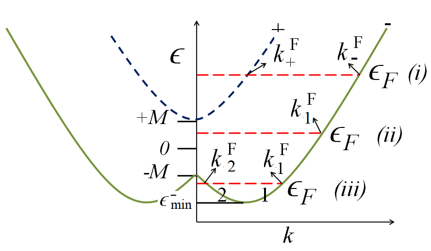
Figure 1: Sketch of spin-split band structure of a 2D Rashba system with a Zeeman like term ($M\sigma_{z}$), when $M<2\epsilon_{\alpha}$.

Here, $k_{\pm}$ represent the radii of the two concentric circular constant energy surfaces. For $\epsilon>M$, the topology of the Fermi surface has convex shape for both $\lambda=+$ and $\lambda=-$ bands. The density of states in each band is given by $D_{\lambda}(\epsilon)=D_{0}(1-\lambda/\tilde{E})$ with $D_{0}=m^{*}/2\pi\hbar^{2}$.

As mentioned earlier, for $\epsilon<-M$ (regime $(iii)$, see Fig. 1), there exists only one energy band $\epsilon_{-}$ and the topology of energy surface is completely different as compared to $\epsilon>M$. For $\epsilon<-M$ and $M<2\epsilon_{\alpha}$, the topology of the Fermi surface has concave-convex shape on the inner and outer branches, respectively. For this regime, the wavevectors are represented by $k_{\nu}=k_{\alpha}\sqrt{[1+(-1)^{\nu-1}\tilde{E}]^{2}-\tilde{M}^{2}}$ with $\nu=1,2$ ($\nu=1\rightarrow$ outer branch and $\nu=2\rightarrow$ inner branch). The DOS in each branch is given by $D_{\nu}=D_{0}|1+(-1)^{\nu-1}/\tilde{E}|$.

For the regime $-M\leq\epsilon\leq M$ (regime $(ii)$, see Fig. 1), only $\nu=1$ branch exists with $\lambda=-1$. Hence the DOS in this branch is given by $D_{\nu=1}=D_{0}(1+1/\tilde{E})$.

The generalized velocity components in the regime $(i)$ are obtained as

$$\langle\hat{v}_{x}\rangle_{\lambda} =\frac{\hbar k_{\alpha}}{m^{*}}\tilde{E}\Big{[}1-\frac{\tilde{M}^{2}}{(\tilde{E}-\lambda)^{2}}\Big{]}^{1/2}\cos\phi+\lambda\frac{\beta E_{y}\tilde{M}}{(\tilde{E}-\lambda)^{3}},$$

$$\langle\hat{v}_{y}\rangle_{\lambda} =\frac{\hbar k_{\alpha}}{m^{*}}\tilde{E}\Big{[}1-\frac{\tilde{M}^{2}}{(\tilde{E}-\lambda)^{2}}\Big{]}^{1/2}\sin\phi-\lambda\frac{\beta E_{x}\tilde{M}}{(\tilde{E}-\lambda)^{3}},$$ (25)

where $\beta=e/(2\hbar k_{\alpha}^{2})$. The velocity components in the regime $(iii)$ with $M<2\epsilon_{\alpha}$ can be obtained from Eq. (III) with $\lambda=-1$ and $\tilde{E}$ replaced by $(-1)^{\nu-1}\tilde{E}$. For the regime $(ii)$ the $\langle\hat{v}_{x}\rangle$ and $\langle\hat{v}_{y}\rangle$ have the similar forms with $\nu=1$.

Similarly, the expectation values of spin velocity operators for the three regimes can be obtained. It is to be noted that the spin velocity $\langle\hat{v}_{xz}\rangle$ and $\langle\hat{v}_{yz}\rangle$ are zero for $M=0$.

For calculating the second order spin currents, we need to know the relaxation time, which is calculated using the framework of semi-classical Boltzmann transport equation including interband and intraband elastic scattering for regime $(i)$, and intrabanch and interbranch scattering within $\lambda=-1$ band for regime $(iii)$ (see Appendix A). The expressions for the relaxation time for the regime $(i)$ are obtained as,

$$\tau_{+} =\frac{4\tau_{0}D_{0}}{A_{+}D_{+}+(B_{+}+P_{+}/R)D_{-}},$$

$$\tau_{-} =\frac{4\tau_{0}D_{0}}{A_{-}D_{-}+(B_{-}+P_{-}R)D_{+}},$$ (26)

where $D_{\lambda}$ is the DOS, $\tau_{0}=2\pi n_{i}mV_{0}^{2}D_{0}/\hbar$, $A_{\lambda}=1+3c_{k_{\lambda}}^{2}$, $B_{\lambda}=2(1-c_{k_{\lambda}}c_{k_{\lambda^{\prime}}})$, $P_{\lambda}=s_{k_{\lambda}}s_{k_{\lambda^{\prime}}}v_{b}^{\lambda^{\prime}}/v_{b}^{\lambda}$, and $R=[D_{-}(A_{-}-P_{+})+D_{+}B_{-}]/[D_{+}(A_{+}-P_{-})+D_{-}B_{+}]$. Similarly, for the regime $(iii)$ the relaxation times are obtained as

$$\tau_{1} =\frac{4\tau_{0}D_{0}}{A_{1}D_{1}+(B_{1}-P_{1}/R)D_{2}},$$

$$\tau_{2} =\frac{4\tau_{0}D_{0}}{A_{2}D_{2}+(B_{2}-P_{2}R)D_{1}},$$ (27)

where $D_{\nu}$ is the DOS in each branch, $A_{\nu}=1+3c_{k_{\nu}}^{2}$, $B_{\nu}=2(1+c_{k_{\nu}}c_{k_{\nu^{\prime}}})$, $P_{\nu}=s_{k_{\nu}}s_{k_{\nu}^{\prime}}v_{b}^{\nu^{\prime}}/v_{b}^{\nu}$, and $R=[D_{2}(A_{2}+P_{1})+D_{1}B_{2}]/[D_{1}(A_{1}+P_{2})+D_{2}B_{1}]$. For the regime $(ii)$, only $\nu=1$ branch persists. Thus, there exists only the intrabranch scattering and hence the relaxation time is $\tau_{-}=4\tau_{0}D_{0}/D_{1}A_{1}$. The analytical expressions for $\tau_{\lambda}$ and $\tau_{\nu}$ in terms of $\epsilon$ are cumbersome, thus not given here.

III.1 Background spin current

Fisrt we present the results for the non-propagating background spin current [22]. It can be easily shown that $\mathcal{J}_{xx}^{(0)}=\mathcal{J}_{yy}^{(0)}=0$. Similarly, $\mathcal{J}_{xz}^{(0)}=\mathcal{J}_{yz}^{(0)}=0$. On the other hand, we obtain $\mathcal{J}_{xy}^{(0)}=-\mathcal{J}_{yx}^{(0)}\neq 0$. At zero temperature $\mathcal{J}_{xy}^{(0)}$ [in units of $\mathcal{J}_{0}=-\hbar^{2}k_{\alpha}^{3}/(24\pi m^{*})$] has the following form

$$\mathcal{J}_{xy}^{(0)} = 4,\;\epsilon_{F}\geq M,$$ (28)

$$\mathcal{J}_{xy}^{(0)} = (2+3\tilde{E}_{F}-\tilde{E}_{F}^{3}-2\tilde{M}^{3}$$

$$+ 3\tilde{E}_{F}\tilde{M}^{2}),\;-M\leq\epsilon_{F}\leq M,$$

$$\mathcal{J}_{xy}^{(0)} = 2\tilde{E}_{F}(3-\tilde{E}_{F}^{2}+3\tilde{M}^{2}),\;\epsilon_{F}\leq-M,$$

where $\tilde{E}_{F}=\sqrt{1+\tilde{\epsilon}_{F}+\tilde{M}^{2}}$ with $\tilde{\epsilon}_{F}=\epsilon_{F}/\epsilon_{\alpha}$. The background spin current $\mathcal{J}_{xy}^{(0)}$ (in units of $\mathcal{J}_{0}$) as a function of rescaled Fermi energy $\tilde{\epsilon}_{F}$ for different values of $\tilde{M}$ is shown in Fig. (2). When $\epsilon_{F}\geq M$ (or $\tilde{\epsilon}_{F}\geq 2\tilde{M}$, i.e. regime $(i)$), the background spin current is independent of $M$ and $\epsilon_{F}$, whereas in the other two regimes, it depends on $M$ and $\epsilon_{F}$. Moreover, $\mathcal{J}_{xy}^{(0)}$ with $M\neq 0$ shows nonmonotonic behavior for $\epsilon_{F}<M$ (regime $(ii)$ and $(iii)$). The background spin current attains a maximum value $\mathcal{J}_{\rm max}^{(0)}=2\mathcal{J}_{0}[1+(1+\tilde{M}^{2})^{3/2}-\tilde{M}^{3}]$ at $\epsilon_{F}=0$ and vanishes at $\epsilon_{F}=\epsilon_{\rm min}^{-}$. The zeroth-order spin current is continuous, while their first and second derivatives are discontinuous at the band edges $\tilde{\epsilon}_{F}=\pm 2\tilde{M}$.

It is instructive to compare these results with the results for $M=0$ case [22]: $\mathcal{J}_{xy}^{(0)}=4\mathcal{J}_{0}$ for $\epsilon_{F}\geq 0$ and $\mathcal{J}_{xy}^{(0)}=2\mathcal{J}_{0}\sqrt{1+\tilde{\epsilon}_{F})}(2-\tilde{\epsilon}_{F})$ for $\epsilon_{F}\leq 0$. These two equations and their first derivatives are continuous; and the second derivative is discontinuous at $\epsilon_{F}=0$.

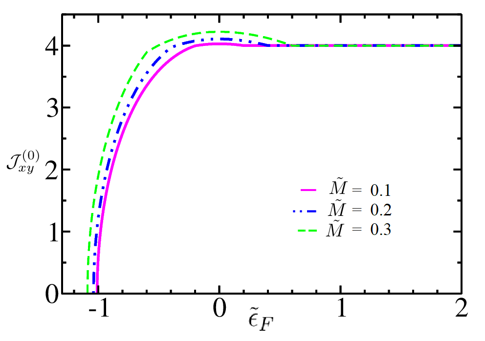
Figure 2: The background spin current $\mathcal{J}_{xy}^{(0)}$ (in units of $\mathcal{J}_{0}$) as a function of rescaled Fermi energy $\tilde{\epsilon}_{F}$ for different values of $\tilde{M}$.

III.2 Linear spin Hall current

Here, we present the results of linear spin current calculated using Eq. (15) for all possible combinations, where we find that $\mathcal{J}_{xx}^{(1),\eta}=\mathcal{J}_{xy}^{(1),\eta}=\mathcal{J}_{yx}^{(1),\eta}=\mathcal{J}_{yy}^{(1),\eta}=0$ and $\mathcal{J}_{xz}^{(1),y}=-\mathcal{J}_{yz}^{(1),x}$. The above results reveal that the electric fields cannot drive linear spin currents having in-plane spin polarization, whereas it can produce linear spin currents having out-of-plane spin polarization. The linear spin current is always transverse to the electric field direction.

The expression for $\mathcal{J}_{xz}^{(1),y}$ ($=\mathcal{J}_{xz,a}^{(1),y}$) at zero temperature is obtained as

$$\mathcal{J}_{xz}^{(1),y} = -\frac{eE_{0}}{8\pi}\frac{(2\tilde{M}^{2}-\tilde{M}^{2}\tilde{\epsilon}_{F}-\tilde{\epsilon}_{F}^{2})}{(\tilde{\epsilon}_{F}+\tilde{M}^{2})^{2}},\;\epsilon_{F}\geq M,$$ (29)

$$\mathcal{J}_{xz}^{(1),y} = \frac{-eE_{0}}{16\pi}\Big{[}\frac{\tilde{M}^{2}}{(1+\tilde{E}_{F})^{2}}-1\Big{]}\hskip 1.4457pt\hskip 1.4457pt,\;-M\leq\epsilon_{F}\leq M,$$

$$\mathcal{J}_{xz}^{(1),y} = \frac{eE_{0}}{4\pi}\frac{\tilde{M}^{2}\tilde{E}_{F}}{(\tilde{\epsilon}_{F}+\tilde{M}^{2})^{2}},\;\epsilon_{F}\leq-M.$$

The linear spin current transverse to the electric field arising solely from the non-zero Berry curvature is the well known spin Hall current. This spin Hall current can be reversed by changing the electric field direction $\bf{E}$ to $-\bf{E}$. The spin Hall conductivity can be defined as $\sigma_{s}=\mathcal{J}_{xz,a}^{(1),y}/E_{0}$. For $\epsilon_{F}\gg M$, the spin Hall conductivity is obtained as $\sigma_{s}^{0}=e/8\pi$, which is exactly the same as obtained by using the Kubo formula for $M\rightarrow 0$ case by various groups [40, 56] previously. However, this universal result vanishes in presence of an arbitrary weak disorder [57]. Reference [58] also justifies this disappearance of static spin-Hall conductivity for any non-vanishing disorder strength in case of the momentum-dependent Rashba strength and non-parabolic energy spectrum. Electron-electron interaction also modifies this universal value of spin Hall conductivity [58]. Similar disorder effect can be performed on our calculation, which may provide the correction terms in the expressions of spin Hall conductivity.

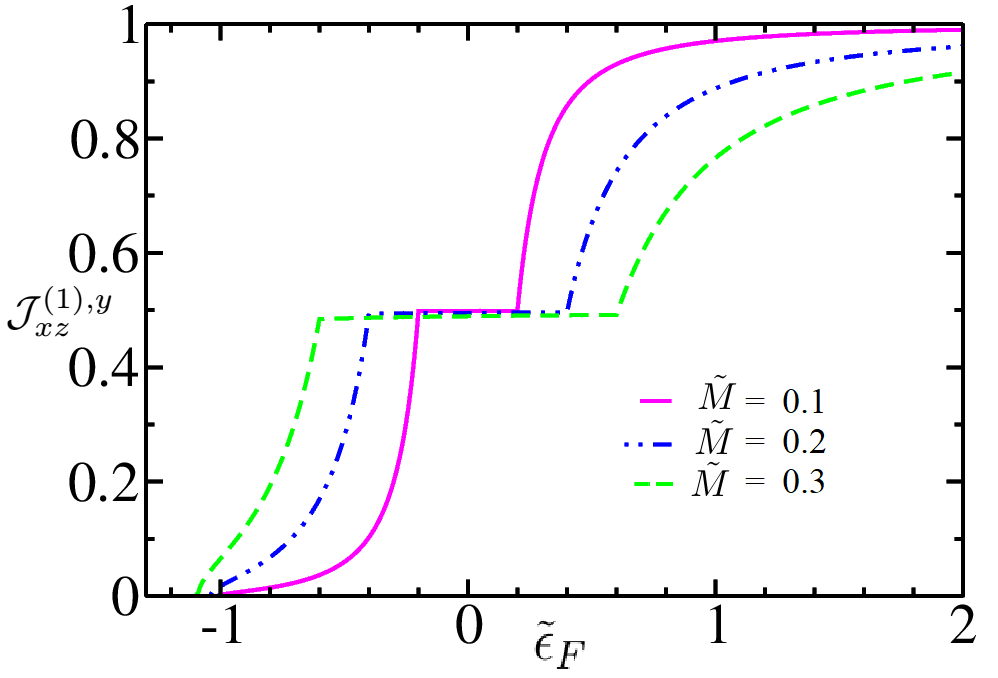
Figure 3: The spin Hall current $\mathcal{J}_{xz}^{(1),y}$ (in units of $\mathcal{J}_{1}=\sigma_{s}^{0}E_{0}$) as a function of rescaled Fermi energy $\tilde{\epsilon}_{F}$ for different values of $\tilde{M}$.

The linear spin Hall current $\mathcal{J}_{xz}^{(1),y}$ (in units of $\mathcal{J}_{1}=\sigma_{s}^{0}E_{0}$) as a function of $\tilde{\epsilon}_{F}$ for different values of $\tilde{M}$ is shown in Fig. (3). It is interesting to note that the spin Hall current displays nearly quantized plateau at $\mathcal{J}_{xz}^{(1),y}=(\mathcal{J}_{xz}^{(1),y})/2$ (i.e. half of the maximum value of spin Hall current) when Fermi energy lies between the two gap edges, i.e. $-2\tilde{M}<\tilde{\epsilon}_{F}<2\tilde{M}$. It reminds us the half-quantized anomalous charge Hall conductance in gapped Rashba systems [54, 55]. Further, $\mathcal{J}_{xz}^{(1),y}$ decreases with increase of $\tilde{M}$ when $\tilde{\epsilon}_{F}>2\tilde{M}$, but it increases with increase of $\tilde{M}$ when $\tilde{\epsilon}_{F}<-2\tilde{M}$.

III.3 Non-linear spin current

In the previous sub-section, it is seen that a finite transverse linear spin current exists while the longitudinal one vanishes. The first non-vanishing contribution to longitudinal spin current in this system is quadratic in E, as is the feature of IS-broken systems. In this sub-section, the quadratic spin current has been studied for all possible configurations of spin orientation, directions of charge propagation and applied electric field. First, we present results where only band velocity contributes to the quadratic spin current and then we show that current with certain spin polarization arises only due to Berry curvature.

Results for $\mathcal{J}_{xy}^{(2),\eta}$: First we consider the quadratic spin current $\mathcal{J}_{xy}^{(2),x}$, so that only the band velocity contributes. It is to be noted that although a Hall field sets up along $\hat{y}$ direction due to anomalous drift of carriers, its contribution to nonlinear spin current ($\mathcal{J}_{xy}^{(2),y}$) is negligible as compared to that of the applied field, and hence not considered throughout the paper.

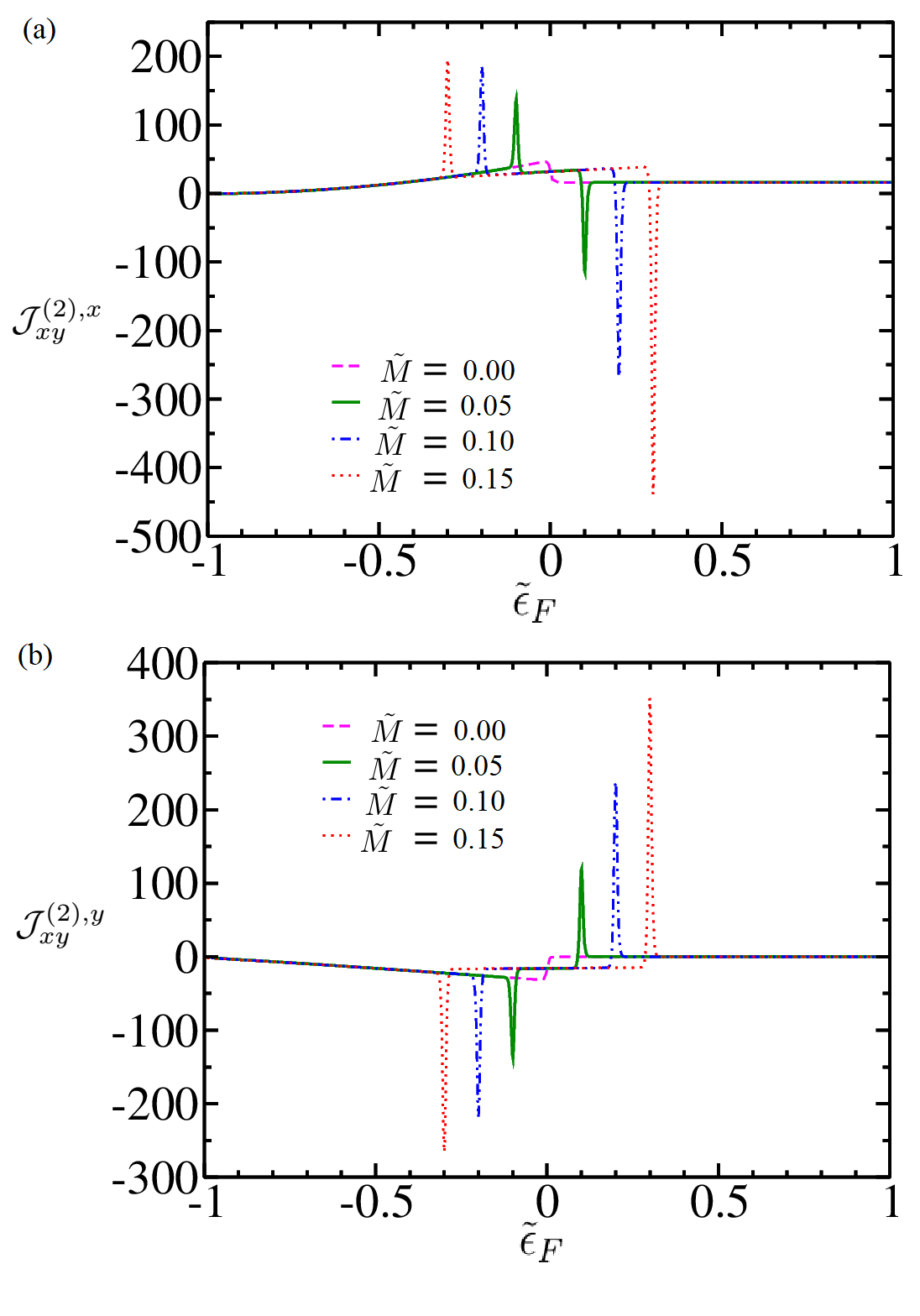
Figure 4: The non-linear spin current (a) $\mathcal{J}_{xy}^{(2),x}$, and (b)$\mathcal{J}_{xy}^{(2),y}$ in units of $\mathcal{J}_{2}$ as a function of $\tilde{\epsilon}_{F}$ for different values of $\tilde{M}$.

We present $\mathcal{J}_{xy}^{(2),x}$ as a function of $\tilde{\epsilon}_{F}$ for different values of $\tilde{M}$ in Fig. (4a). The spin current is independent of the Fermi energy as well as $M$ when $\tilde{\epsilon}_{F}>2\tilde{M}$. For the regime $-2\tilde{M}<\tilde{\epsilon}_{F}<2\tilde{M}$ and $\tilde{\epsilon}_{F}<-2\tilde{M}$, the spin current is independent of $M$, but depends on the Fermi energy. The spin current starts decreasing when $\tilde{\epsilon}_{F}<-2\tilde{M}$. There are two peaks with their values opposite in sign appearing at the gap edges, i.e, at $\tilde{\epsilon}_{F}=\pm 2\tilde{M}$. The absolute value of peak at $\tilde{\epsilon}_{F}=+2\tilde{M}$ is greater than that of the $\tilde{\epsilon}_{F}=-2\tilde{M}$. Further, the peak value increases with the increasing strength of $\tilde{M}$. There is a sharp transition in the spin current around $\epsilon_{F}=0$ when $M=0$. For $M=0$, using the formula in Eq. (17), the spin current $\mathcal{J}_{xy}^{(2),x}$ at zero temperature is obtained as

$$\mathcal{J}_{xy}^{(2),x} =16\mathcal{J}_{2},\;\epsilon_{F}>0,$$

$$\mathcal{J}_{xy}^{(2),x} =\mathcal{J}_{2}\sqrt{1+\tilde{\epsilon_{F}}}\Big{[}48+72\tilde{\epsilon}_{F}+21\tilde{\epsilon}_{F}^{2}\Big{]},\;\epsilon_{F}<0,$$ (30)

where $\mathcal{J}_{2}=(e\tau_{0}E_{0}/\hbar)^{2}\alpha/(32\pi)$ with $\tau_{0}$ being unit of scattering time.

When electric field is directed along $\hat{y}$ direction (${\bf E}=E_{y}\hat{y}$), the anomalous component ($\propto E_{y}$) of spin velocity, i.e, $v_{a,xy}$ exists. However, this anomalous spin velocity gives no net contribution to non-linear spin current. So, $\mathcal{J}_{xy}^{(2),y}$ appears from band component only. The plots for $\mathcal{J}_{xy}^{(2),y}$ as a function of $\tilde{\epsilon}_{F}$ for different values of $\tilde{M}$ is shown in Fig. 4(b). Similar to the previous case, two peaks appear at $\tilde{\epsilon}_{F}=\pm 2\tilde{M}$. Here, at $\tilde{\epsilon}_{F}=-2\tilde{M}$ the peak values are negative and positive at $\tilde{\epsilon}_{F}=+2\tilde{M}$, thereby following opposite trend of spin current when electric field is directed in $\hat{x}$ direction. Thus, the polarization of these currents are opposite when driven by ${\bf E}=E_{0}\hat{x}$ and ${\bf E}=E_{0}\hat{y}$. For $M=0$, the analytical expressions of spin current $\mathcal{J}_{xy}^{(2),y}$ at zero temperature is obtained as

$$\mathcal{J}_{xy}^{(2),y} =0,\;\epsilon_{F}>0,$$

$$\mathcal{J}_{xy}^{(2),y} =-\mathcal{J}_{2}\sqrt{1+\tilde{\epsilon}_{F}}\Big{[}32+16\tilde{\epsilon}_{F}-7\tilde{\epsilon}_{F}^{2}\Big{]},\;\epsilon_{F}<0.$$ (31)

Thus, for the electric field in $\hat{y}$ direction, the spin current propagating in the $\hat{x}$ direction with the polarization in $\hat{y}$ direction is zero for $\epsilon_{F}>0$, whereas it is non-zero for $\epsilon_{F}<0$. When $\epsilon_{F}>0$, the contribution from $\lambda=+$ and $\lambda=-$ bands are same in magnitude but opposite in sign, so their net contribution vanishes. However, it does not vanish when the relaxation time is taken to be constant.

Results for $\mathcal{J}_{yx}^{(2),\eta}$:

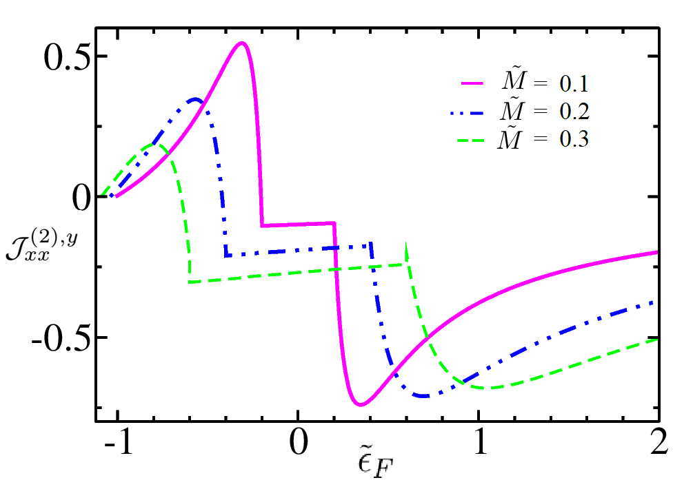
Figure 5: The spin current $\mathcal{J}_{xx}^{(2),y}$ (in units of $\mathcal{J}_{2}^{\prime}$) arising from the anomalous velocity as a function of $\tilde{\epsilon}_{F}$ for different values of $\tilde{M}$.

Here we consider the opposite scenario, i.e, $\hat{y}$ directed spin current with polarization in $\hat{x}$ direction. As expected, we find $\mathcal{J}_{a,yx}^{(2),x}=0$ and $\mathcal{J}_{b,yx}^{(2),x}\neq 0$ with $\mathcal{J}_{b,yx}^{(2),x}=-\mathcal{J}_{b,xy}^{(2),y}$ and thereby $\mathcal{J}_{yx}^{(2),x}=-\mathcal{J}_{xy}^{(2),y}$. Similarly, we find $\mathcal{J}_{yx}^{(2),y}=-\mathcal{J}_{xy}^{(2),x}$.

Results for $\mathcal{J}_{xx}^{(2),\eta}$ and $\mathcal{J}_{yy}^{(2),\eta}$: Now we shall present results for quadratic spin currents, $\mathcal{J}_{xx}^{(2),\eta}$ and $\mathcal{J}_{yy}^{(2),\eta}$, when both propagation and polarization are in the same direction. For $\mathcal{J}_{xx}^{(2),x}$, the anomalous component of the spin velocity is zero and contribution from the band velocity is also zero. Thus, we have $\mathcal{J}_{xx}^{(2),x}=0$. Similarly, one can show that $\mathcal{J}_{yy}^{(2),y}=0$.

On the other hand, we obtain that $\mathcal{J}_{b,xx}^{(2),y}$ is also zero, while $\mathcal{J}_{a,xx}^{(2),y}$ would survive. Using the similar analysis, we find that $\mathcal{J}_{a,yy}^{(2),x}$ is finite. Thus, one can generate pure anomalous nonlinear spin currents having propagation and polarization in the same direction, while electric field is in their transverse direction. Because of the isotropic nature of the Berry curvature, we find $\mathcal{J}_{xx}^{(2),y}=\mathcal{J}_{yy}^{(2),x}$. The plot of $\mathcal{J}_{xx}^{(2),y}$ ($=\mathcal{J}_{a,xx}^{(2),y}$) (in units of $\mathcal{J}_{2}^{\prime}$, where $\mathcal{J}_{2}^{\prime}=(\mathcal{J}_{2}\hbar)/(\tau_{0}\alpha k_{\alpha}))$ as a function of $\tilde{\epsilon}_{F}$ is shown in Fig. (5). It displays that $\mathcal{J}_{xx}^{(2),y}$ is nearly flat when $-2\tilde{M}<\tilde{\epsilon_{F}}<2\tilde{M}$. The appearance of nonlinear anomalous spin current is reminiscent of Berry curvature induced nonlinear charge current which arises from the dipole moment of the Berry curvature [53, 59].

Results for $\mathcal{J}_{xz}^{(2),\eta}$ and $\mathcal{J}_{yz}^{(2),\eta}$: It is not possible to generate quadratic spin current having polarization in $\hat{z}$ direction, as we find $\mathcal{J}_{xz}^{(2),\eta}=\mathcal{J}_{yz}^{(2),\eta}=0$ .

All the above results of spin current (whether it is zero or non-zero) for a 2D gapped Rashba system are tabulated in Table I.

Spin current	${\bf E}=0$	$\eta=x$ (B)	$\eta=x$ (A)	$\eta=y$ (B)	$\eta=y$ (A)
$\mathcal{J}_{xx}^{(0)}$	0	NA	NA	NA	NA
$\mathcal{J}_{xy}^{(0)}$	Finite	NA	NA	NA	NA
$\mathcal{J}_{xz}^{(0)}$	0	NA	NA	NA	NA
$\mathcal{J}_{xx}^{(1),\eta}$	NA	0	0	0	0
$\mathcal{J}_{xy}^{(1),\eta}$	NA	0	0	0	0
$\mathcal{J}_{xz}^{(1),\eta}$	NA	0	0	0	Finite
$\mathcal{J}_{xx}^{(2),\eta}$	NA	0	0	0	Finite
$\mathcal{J}_{xy}^{(2),\eta}$	NA	Finite	0	Finite (for $\epsilon_{F}<0$)	0
$\mathcal{J}_{xz}^{(2),\eta}$	NA	0	0	0	0

*NA: Not Applicable, *B: Band component contribution, *A: Anomalous component contribution

Table 1: Nature of spin currents in 2D gapped Rashba system for different orientations of electric field ${\bf E}$.

Here in Fig. 6, we compare the magnitudes of different orders of spin currents for a 2D gapped Rashba system with $E_{0}=10^{3}$ V/m, $\tau_{0}=2.5$ ps, $m^{*}=0.3m_{e}$ ($m_{e}$: electronic mass), $\alpha=0.1$ eV-nm, and $\tilde{M}=0.1$.

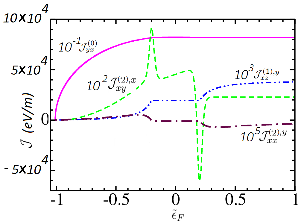
Figure 6: Comparison between the magnitudes of spin currents for different orders in a 2D gapped Rashba system.

IV 3D noncentrosymmetric system

We consider 3D noncentrosymmetric metals such as Li₂(Pd_3-xPt_x)B and B20 compounds having cubic crystal structure. Based on symmetry analysis [62, 61, 60], the Hamiltonian for low-energy conduction electron is given by

$$H=\frac{\hbar^{2}{\bf k}^{2}}{2m^{*}}\sigma_{0}+\alpha\boldsymbol{\sigma}\cdot{\bf k}.$$ (32)

Here ${\bf k}=k(\sin\theta\cos\phi,\sin\theta\sin\phi,\cos\theta)$ is the 3D Bloch wavevector and $\alpha$ is the strength of the linear spin-orbit coupling. Comparing Eq. (32) with Eq. (1), we have $d_{i}=\alpha k_{i}$ with $i=x,y,z$ and the energy spectrum is given by

$$\epsilon_{\lambda}({\bf k})=\frac{\hbar^{2}k^{2}}{2m^{*}}+\lambda\alpha k,$$ (33)

where $\lambda=\pm$ denotes two chiral bands. The band $\epsilon_{-}({\bf k})$ has a minimum energy $\epsilon_{\rm min}=-\epsilon_{\alpha}$ at $k_{\alpha}$. Using the eigenstates given in Eq. (7), the Berry curvature corresponding to $\lambda$ band is given as

$${\boldsymbol{\Omega}}_{\lambda}=-\lambda\frac{{\bf k}}{2k^{3}}.$$ (34)

The spin-momentum locking follows the constraint $\langle{\boldsymbol{\sigma}}\rangle_{\lambda}\cdot{\bf k}=\lambda k$ (or $\langle{\boldsymbol{\sigma}}\rangle_{\lambda}\times{\bf k}=0$), which is completely opposite to the 2D case. Here we would like to mention that in 3D system, a gap in dispersion can’t be created by adding Zeeman term and hence it is neglected in our calculation.

Using the Heisenberg’s equation of motion, the band velocity operator is given by ${\bf\hat{v}}_{b}=\frac{\hbar{\bf k}}{m^{*}}\sigma_{0}+\frac{\alpha}{\hbar}{\boldsymbol{\sigma}}$. The band velocity expression for a given energy $\epsilon\geq 0$, is ${\bf v}_{b}=v_{\alpha}\sqrt{1+\tilde{\epsilon}}\;\hat{\bf k}$ for both the bands $\lambda=\pm$. Here $v_{\alpha}=\hbar k_{\alpha}/m^{*}$, $\tilde{\epsilon}=\epsilon/\epsilon_{\alpha}$ and $\hat{\bf k}={\bf k}/k$ is the unit vector along the vector ${\bf k}$. On contrary, for $\epsilon<0$, the band velocity expression for the two branches $\nu=1,2$ is ${\bf v}_{b}=(-1)^{\nu-1}v_{\alpha}\sqrt{1+\tilde{\epsilon}}\;{\bf\hat{k}}$.

For a given energy $\epsilon\geq 0$, the wavevector corresponding to band $\lambda$ is $k_{\lambda}=k_{\alpha}[-\lambda+\sqrt{1+\tilde{\epsilon}}]$ and the density of states is given by

$$D_{\lambda}(\epsilon)=D_{3}\sqrt{\epsilon_{\alpha}}\Big{[}\frac{2+\tilde{\epsilon}}{\sqrt{1+\tilde{\epsilon}}}-2\lambda\Big{]},$$

where $D_{3}=\frac{1}{4\pi^{2}}(\frac{2m^{*}}{\hbar^{2}})^{3/2}$.

On the other hand, for a given energy $-\epsilon_{\alpha}<\epsilon<0$, the wavevector corresponding to branch $\nu$ is $k_{\nu}=k_{\alpha}[1+(-1)^{\nu+1}\sqrt{1+\tilde{\epsilon}}]$ and the density of states is given by

$$D_{\nu}(\epsilon)=D_{3}\sqrt{\epsilon_{\alpha}}\Big{[}\frac{2+\tilde{\epsilon}}{\sqrt{1+\tilde{\epsilon}}}+2(-1)^{\nu+1}\Big{]}.$$

The energy-dependent relaxation times used for calculating spin currents in 3D non-centrosymmetric metals have the following forms [63]

$$\tau_{\lambda} = \frac{u_{0}}{2D_{3}}\Big{[}\frac{\sqrt{1+\tilde{\epsilon}}}{\sqrt{\epsilon_{\alpha}}(2+\tilde{\epsilon})}\Big{]}\Big{[}1-\lambda\frac{\sqrt{1+\tilde{\epsilon}}}{2+\tilde{\epsilon}}\Big{]},\;\epsilon\geq 0$$ (35)

$$\tau_{\nu} = \frac{u_{0}}{2D_{3}}\Big{[}\frac{\sqrt{1+\tilde{\epsilon}}}{\sqrt{\epsilon_{\alpha}}(2+\tilde{\epsilon})}\Big{]}\Big{[}1+(-1)^{\nu-1}\lambda\frac{\sqrt{1+\tilde{\epsilon}}}{2+\tilde{\epsilon}}\Big{]},\;\epsilon<0,$$

where $1/u_{0}=\pi n_{\rm imp}V_{0}^{2}/\hbar$ with $n_{\rm imp}$ being the impurity density.

IV.1 Background spin current

For a 3D Rashba system, the equilibrium background spin current $\mathcal{J}_{ii}^{(0)}$ with $i=x,y,z$ is obtained as

$$\mathcal{J}_{ii}^{(0)}=\frac{\hbar^{2}k_{\alpha}^{4}}{3\pi^{2}m^{*}}\sqrt{1+\tilde{\epsilon}_{F}},\;\forall\;\epsilon_{F}.$$ (36)

Thus, the background spin current and its derivative are continuous across the BTP. On the other hand, we find all other components are zero i.e. $\mathcal{J}_{ij}^{(0)}=0$ with $i\neq j$. The nature of background spin current in 3D is completely different from that of 2D Rashba system. For $\tilde{\epsilon}_{F}\gg 1$, $\mathcal{J}_{xx}^{(0)}\sim\alpha^{3}$, but $\mathcal{J}_{xx}^{(0)}\sim\alpha^{4}$ when $\tilde{\epsilon}_{F}\ll 1$.

IV.2 Spin Hall current

Using symmetry analysis, the linear spin current due to the band velocity becomes zero. On the other hand, the anomalous velocity gives rise to linear spin current which propagates transverse to the external electric field. The spin Hall current expression is obtained as $\mathcal{J}_{ij}^{(1),\nu}=\sigma_{\rm s}\epsilon_{ij\nu}E_{\nu}$, where the spin Hall conductivity $\sigma_{\rm s}$ is given by

$$\sigma_{\rm s}=-\frac{e}{12\pi^{2}}k_{\alpha}\sqrt{1+\tilde{\epsilon}_{F}},\;\forall\;\epsilon_{F}.$$ (37)

Here $\epsilon_{ij\nu}$ is the fully antisymmetric Levi-Civita tensor. The same expression of $\sigma_{\rm s}$ can be obtained using the Kubo formula (see Appendix B). For $\tilde{\epsilon}_{F}\gg 1$, $\sigma_{\rm s}\simeq(-e/12\pi^{2})\sqrt{2m^{*}\epsilon_{F}^{0}/\hbar^{2}}$ with $\epsilon_{F}^{0}$ being the Fermi energy for conventional 3D metals. On the other hand, $\sigma_{\rm s}\sim k_{\alpha}$ at the band touching point ${\bf k}=0$.

IV.3 Nonlinear Spin current

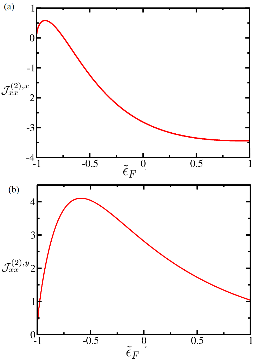
Figure 7: Spin current (a) $\mathcal{J}_{xx}^{(2),x}$, and (b) $\mathcal{J}_{xx}^{(2),y}$ in units of $\mathcal{J}_{3}$ as a function of $\tilde{\epsilon}_{F}$.

Here we present the results of nonlinear spin currents for 3D Rashba system. The off diagonal spin current $\mathcal{J}_{ij}^{(2),\eta}$ with $i\neq j$ from both band and anomalous component of spin velocity are zero, whereas the diagonal spin currents $\mathcal{J}_{ii,b}^{(2),\eta}$ arising from band component have non zero values. The anomalous component of diagonal spin current, i.e, $\mathcal{J}_{ii,a}^{(2),\eta}$ is also zero. Thus, unlike the 2D case (with Zemman term) there is no nonlinear current in 3D due to the anomalous component because of the time reversal symmetry.

Results for $\mathcal{J}_{xx}^{(2),\eta}$: As already mentioned for 3D Rashba system, the nonlinear spin current arises solely from the band component. The spin current $\mathcal{J}_{xx}^{(2),x}$ for a 3D system is obtained as

$$\mathcal{J}_{xx}^{(2),x} = -\mathcal{J}_{3}\frac{\sqrt{1+\tilde{\epsilon}_{F}}}{(2+\tilde{\epsilon}_{F})^{5}}\Big{[}90+239\tilde{\epsilon}_{F}$$

$$+ 199\tilde{\epsilon}_{F}^{2}+58\tilde{\epsilon}_{F}^{3}+5\tilde{\epsilon}_{F}^{4}\Big{]},\;\forall\;\epsilon_{F},$$

where $\mathcal{J}_{3}=(\hbar^{2}eu_{0}E_{0}\pi)^{2}/(30m^{*3})$.

Expression (IV.3) depicts a smooth variation of quadratic spin current across $\epsilon_{F}=0$ (band touching point) in 3D Rashba, which ensures continuity of the first derivative of spin current, unlike its 2D counterpart. This is because the forms of DOS are different for $\epsilon>0$ and $\epsilon<0$ in 2D Rashba, while for 3D case, they are same. The spin current, $\mathcal{J}_{xx}^{(2),x}$ (in units of $\mathcal{J}_{3}$) as a function of $\tilde{\epsilon}_{F}$ is shown in Fig. 7(a) which depicts an increasing trend of spin currents (considering absolute value) with $\tilde{\epsilon}_{F}$, except in the region $-0.9<\tilde{\epsilon}_{F}<-0.75$. The spin current changes sign at $\tilde{\epsilon}_{F}\sim 0.75$.

Now we consider the electric field in $\hat{y}$ direction. Similar to previous case (electric field in $\hat{x}$ direction), here also the spin current arises from band component only. The spin current $\mathcal{J}_{xx}^{(2),y}$ for a 3D system is obtained as

$$\mathcal{J}_{xx}^{(2),y} = \mathcal{J}_{3}\frac{\sqrt{1+\tilde{\epsilon}_{F}}}{(2+\tilde{\epsilon}_{F})^{5}}\Big{[}90+97\tilde{\epsilon}_{F}$$

$$+ 2\tilde{\epsilon}_{F}^{2}-11\tilde{\epsilon}_{F}^{3}\Big{]},\;\forall\;\epsilon_{F}.$$

The plot for $\mathcal{J}_{xx}^{(2),y}$ as a function of $\tilde{\epsilon}_{F}$ is shown in Fig. 7(b). The figure shows that the spin current $\mathcal{J}_{xx}^{(2),y}$ is zero at $\tilde{\epsilon}_{F}=-1$ and then it starts to increase, attends maxima at $\tilde{\epsilon}_{F}\sim-0.6$ and then again decreases. There is no sign change for the considered range of $\tilde{\epsilon}_{F}$.

Similarly, the spin currents $\mathcal{J}_{xx}^{(2),z}$ is obtained, where we find $\mathcal{J}_{xx}^{(2),z}=\mathcal{J}_{xx}^{(2),y}$.

Results for $\mathcal{J}_{yy}^{(2),\eta}$ and $\mathcal{J}_{zz}^{(2)\eta}$: Here we find $\mathcal{J}_{yy}^{(2),x}=\mathcal{J}_{yy}^{(2),z}=\mathcal{J}_{zz}^{(2),x}=\mathcal{J}_{zz}^{(2),y}=\mathcal{J}_{xx}^{(2),y}=\mathcal{J}_{xx}^{(2),z}$. Similarly, we obtain $\mathcal{J}_{yy}^{(2),y}=\mathcal{J}_{zz}^{(2),z}=\mathcal{J}_{xx}^{(2),x}$.

Fig. 8 depicts the comparison of the magnitudes of different orders of spin currents for a 3D Rashba system with $E_{0}=10^{3}$ V/m, $\tau_{0}=u_{0}/(2D_{3}\sqrt{\epsilon_{\alpha}})=2.5$ ps, $m^{*}=0.3m_{e}$ ($m_{e}$: electronic mass), and $\alpha=0.1$ eV-nm.

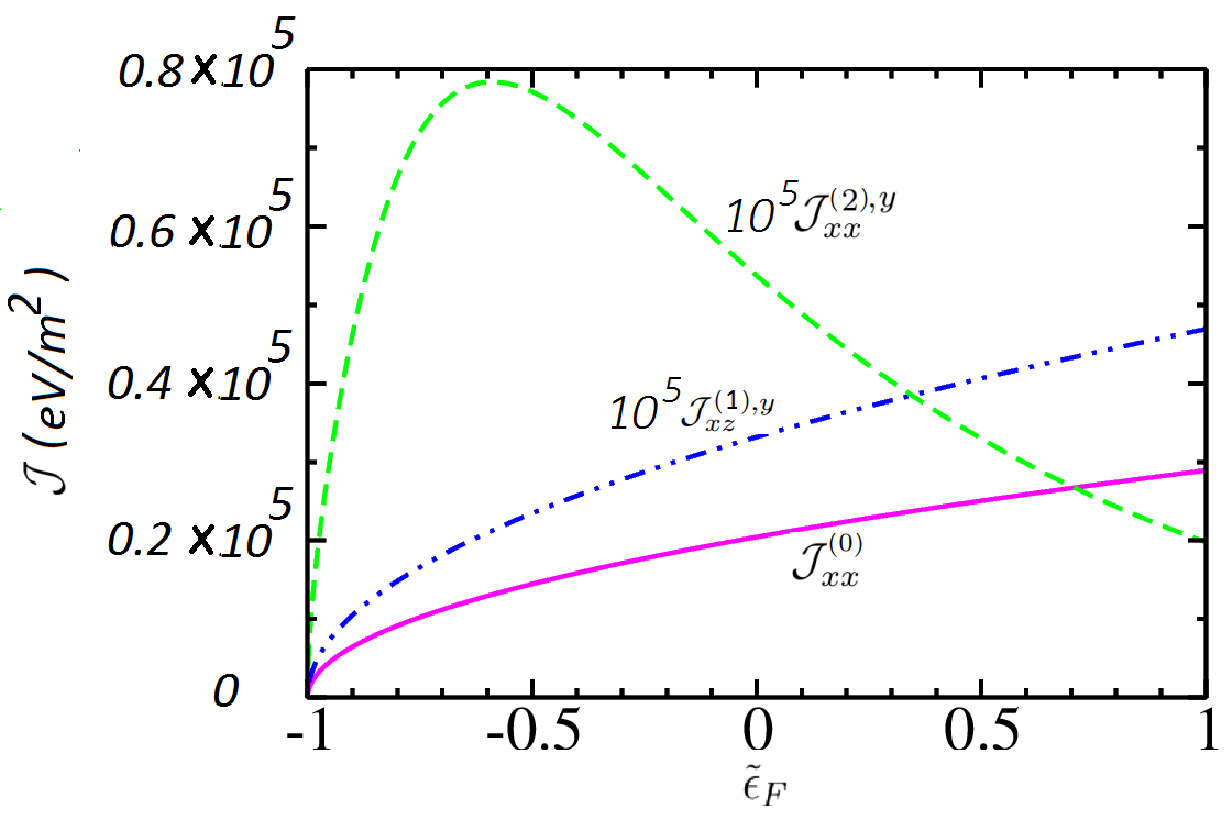
Figure 8: Comparison between the magnitudes of spin currents for different orders in a 3D Rashba system.

The results of spin currents in 3D noncentrosymmetric system are concisely summarized in Table. II.

Spin current	${\bf E}=0$	$\eta=x$ (B)	$\eta=x$ (A)	$\eta=y$ (B)	$\eta=y$ (A)	$\eta=z$ (B)	$\eta=z$ (A)
$\mathcal{J}_{xx}^{(0)}$	Finite	NA	NA	NA	NA	NA	NA
$\mathcal{J}_{xy}^{(0)}$	0	NA	NA	NA	NA	NA	NA
$\mathcal{J}_{xz}^{(0)}$	0	NA	NA	NA	NA	NA	NA
$\mathcal{J}_{xx}^{(1),\eta}$	NA	0	0	0	0	0	0
$\mathcal{J}_{xy}^{(1),\eta}$	NA	0	0	0	0	0	Finite
$\mathcal{J}_{xz}^{(1),\eta}$	NA	0	0	0	Finite	0	0
$\mathcal{J}_{xx}^{(2),\eta}$	NA	Finite	0	Finite	0	Finite	0
$\mathcal{J}_{xy}^{(2),\eta}$	NA	0	0	0	0	0	0
$\mathcal{J}_{xz}^{(2),\eta}$	NA	0	0	0	0	0	0

*NA: Not Applicable, *B: Band component contribution, *A: Anomalous component contribution

Table 2: Nature of spin currents in 3D noncentrosymmetric system for different orientations of electric field ${\bf E}$.

Here we would like to emphasize on the differences of the 2D and 3D results. In case of 2D Rashba system, the spin currents arising from band component always have the polarization and propagation direction perpendicular to each other, whereas in 3D system, the propagation and polarization directions are same. This may be attributed to fact that for 2D case, Rashba spin-orbit interaction ($\alpha\boldsymbol{\sigma}\cdot({\bf k}\times{\bf\hat{z}}$)) locks the spin orientation perpendicular to the momentum and thereby yields no contribution for the spin currents having same propagation and polarization directions. For 3D case, Rashba spin-orbit interaction ($\alpha\boldsymbol{\sigma}\cdot{\bf k}$) locks the spin orientation parallel to the momentum and hence the spin currents having the propagation and polarization directions perpendicular to each other become zero. For 3D case, the expressions for the spin currents depicts a smooth variation across $\epsilon_{F}=0$, unlike the 2D case. This is because of the different forms of DOS for $\epsilon_{F}>0$ and $\epsilon_{F}<0$ in 2D Rashba, while for 3D case, they are same. For 2D gapped Rashba system, the Berry curvature induces pure nonlinear spin current, whereas in 3D system, there is no anomalous nonlinear spin current because of the time reversal symmetry.

V Conclusion

We have studied the background, linear and nonlinear spin currents in 2D Rashba spin-orbit coupled systems with Zeeman coupling and in 3D non-centrosymmetric metals. We have incorporated the correction due to Berry curvature induced anomalous velocity in the semiclassical equations of motion, which contributes to spin currents transverse to the applied field. We have considered energy dependent relaxation time obtained by solving the Boltzmann transport equations self consistently with (i) interband and intraband scattering for $\epsilon>M$, (ii) intrabanch scattering for $-M\leq\epsilon\leq M$ and (iii) interbranch and intrabranch scattering for $\epsilon<-M$ in presence of the short-range impurity.

For 2D Rashba systems, the background spin current has only an in-plane component with spin polarization perpendicular to direction of propagation. It increases with $\epsilon_{F}$ and attains a fixed value (independent of the Zeeman coupling) when Fermi energy is above the ‘Zeeman’ gap. The linear spin current has only a transverse component due to anomalous velocity of carriers. The spin Hall conductivity rises with $\epsilon_{F}$, exhibits a plateau at the Zeeman gap (similar to the Hall plateau) and saturates to the intrinsic value $e/(8\pi)$ at higher $\epsilon_{F}$, which is independent of the Zeeman gap. This linear current has out-of-plane spin polarization. The nonlinear spin current (arising from band component) has both longitudinal and transverse components in general and are polarized in-plane. When $\epsilon_{F}$ is above the gap, the longitudinal part is constant in $\epsilon_{F}$ while the transverse one vanishes. Both the nonlinear components are sharply peaked at the gap edges with opposite spin polarizations at the upper and lower edges. The magnitudes of peak values get enhanced with the strength of the Zeeman coupling. We get pure anomalous nonlinear spin current with polarization along the direction of propagation with extrema near the gap edges.

In 3D noncentrosymmetric metals, the background spin current has spin polarization along the direction of propagation and is an increasing function of $\epsilon_{F}$. The linear spin current has its directions of propagation, spin polarization and applied electric field mutually orthogonal to one another and increases as a function of $\epsilon_{F}$. For very high $\epsilon_{F}$, the linear spin Hall conductance is nearly independent of Rashba coupling strength and varies as $\sqrt{\epsilon_{F}^{0}}$. Both the transverse and longitudinal components of nonlinear spin current have their spin polarization aligned parallel or anti-parallel to the direction of propagation.

Thus, gapped 2D Rashba systems and 3D noncentrosymmetric metals are valuable assets to explore the Berry curvature induced spin currents. The correction due to Berry curvature in the spin velocity operator results in an ‘extrinsic’ spin Hall current and gives an additional $xx$ (or $yy$) component of nonlinear spin current. The magnitudes of these currents in gapped Rashba systems can be controlled by tuning the external magnetic field, which makes it suitable for experimental studies. The plateau of linear spin current and the sharp peaks of nonlinear spin currents may act as probe for detection of Zeeman coupling from magnetic impurities and its corresponding strength in 2D Rashba systems. In 3D noncentrosymmetric metals, the Berry curvature results in linear spin Hall current but does not affect the nonlinear ones.

VI Acknowledgments

P. Kapri thanks Department of Physics, IIT Kanpur, India for financial support.

Appendix A Derivation of Relaxation time for a 2D gapped Rashba system

Here we present the derivation of relaxation time of a gapped 2D Rashba system with spin-independent short-range scatterer using the semiclassical BTE self-consistently. Following Refs. [63, 64], the coupled equations for the relaxation time $\tau_{\zeta}(\epsilon)$ are given by

$$\frac{1}{\tau_{\zeta}(\epsilon)}=\frac{1}{2\pi}\sum_{\zeta^{\prime}}\int d\epsilon_{\zeta^{\prime}}d\phi^{\prime}D_{\zeta^{\prime}}(\epsilon_{\zeta^{\prime}})W_{\zeta^{\prime}\zeta}(\epsilon_{\zeta},\epsilon_{\zeta^{\prime}})\Big{[}1-\cos(\phi^{\prime}-\phi)\frac{v_{b}^{\zeta^{\prime}}\tau_{\zeta^{\prime}}}{v_{b}^{\zeta}\tau_{\zeta}}\Big{]}.$$ (40)

Here $\zeta\equiv(\lambda,{\bf k})$ and $\zeta\equiv(\nu,{\bf k})$ is the eigenstate index for the regime $\epsilon>M$ and $\epsilon_{\rm min}^{-}<\epsilon<-M$ respectively and the transition rate between the states $\zeta$ and $\zeta^{\prime}$ is

$$W_{\zeta^{\prime},\zeta} =\frac{2\pi}{\hbar}\Big{|}\langle\zeta^{\prime}|V({\bf r})|\zeta\rangle\Big{|}^{2}\delta(\epsilon_{\zeta}-\epsilon_{\zeta^{\prime}}),$$

where $V({\bf r})=V_{0}\sum_{i}\delta({\bf r}-{\bf R}_{i})$ with a constant strength $V_{0}$.

After performing the integral and summation of Eq. (40), for the regime $\epsilon>M$, it reduces to

$$\frac{1}{\tau_{\lambda}}=\frac{D_{\lambda}A_{\lambda}}{4\tau_{0}D_{0}}+\frac{D_{\lambda^{\prime}}(B_{\lambda}+(P_{\lambda}\tau_{\lambda^{\prime}})/\tau_{\lambda})}{4\tau_{0}D_{0}},$$ (41)

where $A_{\lambda}=1+3c_{k_{\lambda}}^{2}$, $B_{\lambda}=2(1-c_{k_{\lambda}}c_{k_{\lambda^{\prime}}})=B_{\lambda^{\prime}}$, and $P_{\lambda}=s_{k_{\lambda}}s_{k_{\lambda^{\prime}}}v_{b}^{\lambda^{\prime}}/v_{b}^{\lambda}$. Also, $\tau_{0}=2\pi n_{\rm im}V_{0}^{2}D_{0}/\hbar$ with $n_{\rm im}$ being the impurity concentration and $D_{0}=m^{*}/(2\pi\hbar^{2})$. Solving the coupled equations for $1/\tau_{+}$ and $1/\tau_{-}$, the relaxation times of the two bands for $\epsilon>M$ are obtained as

$$\tau_{+}=\frac{4\tau_{0}D_{0}}{A_{+}D_{+}+(B_{+}+P_{+}/R)D_{-}}\hskip 7.22743pt;\hskip 7.22743pt\tau_{-}=\frac{4\tau_{0}D_{0}}{A_{-}D_{-}+(B_{-}+P_{-}R)D_{+}},$$ (42)

with $R=\frac{D_{-}(A_{-}-P_{+})+D_{+}B_{-}}{D_{+}(A_{+}-P_{-})+D_{-}B_{+}}$.

Similarly, for the regime $\epsilon_{\rm min}^{-}<\epsilon<-M$, the coupled equations for the relaxation time $\tau_{\nu}(\epsilon)$ are

$$\frac{1}{\tau_{\nu}}=\frac{D_{\nu}A_{\nu}}{4\tau_{0}D_{0}}+\frac{D_{\nu^{\prime}}(B_{\nu}-(P_{\nu}\tau_{\nu^{\prime}})/\tau_{\nu})}{4\tau_{0}D_{0}}.$$ (43)

Here $A_{\nu}=1+3c_{k_{\nu}}^{2}$, $B_{\nu}=2(1+c_{k_{\nu}}c_{k_{\nu^{\prime}}})=B_{\nu^{\prime}}$, and $P_{\nu}=s_{k_{\nu}}s_{k_{\nu^{\prime}}}v_{b}^{\nu^{\prime}}/v_{b}^{\nu}$. Solving the Eq. 43, the relaxation times of the two branches for $\epsilon_{\rm min}^{-}<\epsilon<-M$ are obtained as

$$\tau_{1}=\frac{4\tau_{0}D_{0}}{A_{1}D_{1}+(B_{1}-P_{1}/R)D_{2}}\hskip 7.22743pt;\hskip 7.22743pt\tau_{2}=\frac{4\tau_{0}D_{0}}{A_{2}D_{2}+(B_{2}-P_{2}R)D_{1}},$$ (44)

where $R=\frac{D_{2}(A_{2}+P_{1})+D_{1}B_{2}}{D_{1}(A_{1}+P_{2})+D_{2}B_{1}}$.

Appendix B Spin Hall current in 3D noncentrosymmetric system from Kubo formalism

The spin Hall conductivity in a clean 3D Rashba system using Kubo formula [56] is obtained as

$$\sigma_{\rm s} = \frac{e\hbar^{2}}{2}\sum_{\lambda\neq\lambda^{\prime}}\int\frac{d^{3}\bf{k}}{(2\pi)^{3}}(f_{k_{\lambda^{\prime}}}-f_{k_{\lambda}})Im\frac{\langle k,\lambda^{\prime}|\hat{v}_{xz}|k,\lambda\rangle\langle k,\lambda^{\prime}|\hat{v}_{y}|k,\lambda\rangle}{(\epsilon_{k_{\lambda}}-\epsilon_{k_{\lambda^{\prime}}})^{2}}$$

$$= \frac{e\hbar^{2}}{4m^{*}\alpha}\int\frac{d^{3}\bf{k}}{(2\pi)^{3}}(f_{-}-f_{+})\frac{\sin^{2}\theta\cos^{2}\phi}{k}=\frac{ek_{\alpha}}{12\pi^{2}}\sqrt{1+\tilde{\epsilon}_{F}}.$$

References

- [1] S. A. Wolf, D. D. Awschalom, R. A. Buhrman, J. M. Daughton, S. von Molnar, M. L. Roukes, A. Y. Chtchelkanova, D. M. Treger, Science 294, 1488 (2001).
- [2] I. Zutic, J. Fabian, and S. Das Sarma, Rev. Mod. Phys. 76, 323 (2004).
- [3] S. D. Bader and S. S. P. Parkin, Annu. Rev. Condens. Matter Phys 1, 71 (2010).
- [4] J. Schliemann, Rev. Mod. Phys. 89, 011001 (2017).
- [5] S. Datta and B. Das, App. Phys. Lett. 56, 665 (1990).
- [6] S. Gardelis, C. G. Smith, C. H. W. Barnes, E. H. Linfield, and D. A. Ritchie, Phys. Rev. B 60, 7764 (1999).
- [7] G. Schmidt, D. Ferrand, L. W. Molenkamp, A. T. Filip, and B. J. van Wees, Phys. Rev. B 62, R4790 (2000).
- [8] C. M. Hu, J. Nitta, A. Jensen, J. B. Hansen, and H. Takayanagi, Phys. Rev. B 63, 125333 (2001).
- [9] N. Tombros, C. Jozsa, M. Popinciuc, H. T. Jonkman, and B. J. v. Wees, Nature (London) 448, 571 (2007).
- [10] J. Xiao, G. E. W. Bauer, K. Uchida, E. Saitoh, and S. Maekawa, Phys. Rev. B 81, 214418 (2010).
- [11] E. Saitoh, M. Ueda, H. Miyajima, and G. Tatara, App. Phys. Lett. 88, 182509 (2006).
- [12] K. Ando, S. Takahashi, J. Ieda, H. Kurebayashi, T. Trypiniotis, C. H. W. Barnes, S. Maekawa, and E. Saitoh, Nat. Mat. 10, 655 (2011).
- [13] S. Dushenko, H. Ago, K. Kawahara, T. Tsuda, S. Kuwabata, T. Takenobu, T. Shinjo, Y. Ando, and M. Shiraishi, Phys. Rev. Lett. 116, 166102 (2016).
- [14] E. Lesne, Y. Fu, S. Oyarzun, J. C. Rojas-Sanchez, D. C. Vaz, H. Naganuma, G. Sicoli, J.-P. Attane, M. Jamet, E. Jacquet, J.-M. George, A. Barthélémy, H. Jaffres, A. Fert, M. Bibes, and L. Vila, Nat. Mat. 15, 1261 (2016).
- [15] K. Kondou, R. Yoshimi, A. Tsukazaki, Y. Fukuma, J. Matsuno, K. S. Takahashi, M. Kawasaki, Y. Tokura, and Y. Otani, Nat. Phys. 12, 1027 (2016).
- [16] S. D. Ganichev, E. L. Ivchenko, V. V. Bel’kov, S. A. Tarasenko, M. Sollinger, D. Weiss, W. Wegscheider, and W. Prettl, Nature (London) 417, 153 (2002).
- [17] M. J. Stevens, A. L. Smirl, R. D. R. Bhat, A. Najmaie, J. E. Sipe, and H. M. van Driel, Phys. Rev. Lett. 90, 136603 (2003).
- [18] E. I. Rashba, Sov. Phys. Solid State 2, 1109 (1960).
- [19] Y. A. Bychkov and E. I. Rashba, J. Phys. C 17, 6039 (1984).
- [20] J. Nitta, T. Akazaki, H. Takayanagi, and T. Enoki, Phys. Rev. Lett. 78, 1335 (1997).
- [21] G. Engels, J. Lange, T. Schapers, and H. Luth, Phys. Rev. B 55, 1958 (1997).
- [22] E. I. Rashba, Phys. Rev. B 68, 241315 (2003).
- [23] E. I. Rashba, Phys. Rev. B 70, 161201(R) (2004).
- [24] J. Shi, P. Zhang, D. Xiao, and Q. Niu, Phys. Rev. Lett. 96, 076604 (2006).
- [25] Q.-F. Sun and X. C. Xie, Phys. Rev. B 72, 245305 (2005).
- [26] Y. Wang, K. Xia, Z.-B. Su, and Z. Ma, Phys. Rev. Lett. 96, 066601 (2006).
- [27] J. Wang, B. Wang, W. Ren, and H. Guo, Phys. Rev. B 74, 155307 (2006).
- [28] Q. Sun, X. C. Xie, and J. Wang, Phys. Rev. B 77, 035327 (2008).
- [29] D. Loss, P. Goldbart, and A. V. Balatsky, Phys. Rev. Lett. 65, 1655 (1990).
- [30] J. Splettstoesser, M. Governale, and U. Zülicke, Phys. Rev. B 68, 165341 (2003).
- [31] F. Schutz, M. Kollar, and P. Kopietz, Phys. Rev. Lett. 91, 017205 (2003).
- [32] Usaj and C. A. Balseiro, Europhys. Lett. 72, 631 (2005).
- [33] F. Dolcini and F. Rossi, Phys. Rev. B 98, 045436 (2018).
- [34] L. Rossi, F. Dolcini, and F. Rossi, Phys. Rev. B 101, 195421 (2020).
- [35] Q. -F. Sun, H. Guo, and J. Wang, Phys. Rev. B 69, 054409 (2004).
- [36] E. B. Sonin, Phys. Rev. Lett. 99, 266602 (2007).
- [37] D. G. Newman, M. Dabrowski, and P. S. Keatley, Q. Li, M. Yang, S. R. Marmion, B. J. Hickey, Z.-Q. Qiu, R. J. Hicken, IEEE Transactions on Magnetics 57, 1 (2021).
- [38] S. Murakami, N. Nagaosa, and S. C. Zhang, Science 301, 1348 (2003).
- [39] S. Murakami, N. Nagaosa, and S. C. Zhang, Phys. Rev. B 69, 235206 (2004).
- [40] J. Sinova, D. Culcer, Q. Niu, N. A. Sinitsyn, T. Jungwirth, and A. H. MacDonald, Phys. Rev. Lett. 92, 126603 (2004).
- [41] J. Wunderlich, B. Kaestner, J. Sinova, and T. Jungwirth, Phys. Rev. Lett. 94, 047204 (2005).
- [42] B. Paul and T. K. Ghosh, Phys. Lett. A 379, 728 (2015).
- [43] J. E. Hirsch, Phys. Rev. Lett. 83, 1834 (1999).
- [44] S. Zhang, Phys. Rev. Lett. 85, 393 (2000).
- [45] Y. K. Kato, R. C. Myers, A. C. Gossard, and D. D. Awschalom, Science 306, 1910 (2004).
- [46] C. Day, Phys. Today 58, 17 (2005).
- [47] K. Hamamoto, M. Ezawa, K. W. Kim, T. Morimoto, and N. Nagaosa, Phys. Rev. B 95, 224430 (2017).
- [48] H. Yu, Y. Wu, G. Liu, X. Xu, and W. Yao, Phys. Rev. Lett. 113, 156603 (2014).
- [49] A. Pan and D. C. Marinescu, Phys. Rev. B 99, 245204 (2019).
- [50] Y. Gao, S. A. Yang, and Q. Niu, Phys. Rev. B 95, 165135 (2017).
- [51] M.-C Chang and Qian Niu, Phys. Rev. Lett. 75, 1348 (1995).
- [52] G. Sundaram and Q. Niu, Phys. Rev. B 59, 14915 (1999).
- [53] I. Sodemann and L. Fu, Phys. Rev. Lett. 115, 216806 (2015).
- [54] D. Culcer, A. MacDonald, and Q. Niu, Phys. Rev. B 68, 045327 (2003).
- [55] T. Ojanen and T. Kitagawa, Phys. Rev. B 85, 161202(R) (2012).
- [56] C. P. Moca and D. C. Marinescu, New J. Phys. 9, 343 (2007).
- [57] E. G. Mishchenko, A. V. Shytov, and B. I. Halperin, Phys. Rev. Lett. 93, 226602 (2004).
- [58] O. V. Dimitrova, Phys. Rev. B 71, 245327 (2005).
- [59] S. Nandy and I. Sodemann, Phys. Rev. B 100, 195117 (2019).
- [60] K.-W. Lee and W. E. Pickett, Phys. Rev. B 72, 174505 (2005).
- [61] K. V. Samokhin, Phys. Rev. B 78, 144511 (2008).
- [62] J. Kang and J. Zang, Phys. Rev. B 91, 134401 (2015).
- [63] S. Verma, T. Biswas, and T. K. Ghosh, Phys. Rev. B 100, 045201 (2019).
- [64] C. Xiao, D. L, and Z. Ma, Phys. Rev. B 93, 075150 (2016).