The Effects of Three-dimensional Radiative Transfer
on the Resonance Polarization of the Ca i 4227 $\mathrm{\AA}$ line

Abstract

The sizable linear polarization signals produced by the scattering of anisotropic radiation in the core of the Ca i 4227 Å line constitute an important observable for probing the inhomogeneous and dynamic plasma of the lower solar chromosphere. Here we show the results of a three-dimensional (3D) radiative transfer complete frequency redistribution (CRD) investigation of the line’s scattering polarization in a magneto-hydrodynamical 3D model of the solar atmosphere. We take into account not only the Hanle effect produced by the model’s magnetic field, but also the symmetry breaking caused by the horizontal inhomogeneities and macroscopic velocity gradients. The spatial gradients of the horizontal components of the macroscopic velocities produce very significant forward scattering polarization signals without the need of magnetic fields, while the Hanle effect tends to depolarize them at the locations where the model’s magnetic field is stronger than about 5 G. The standard 1.5D approximation is found to be unsuitable for understanding the line’s scattering polarization, but we introduce a novel improvement to this approximation that produces results in qualitative agreement with the full 3D results. The instrumental degradation of the calculated polarization signals is also investigated, showing what can we expect to observe with the Visible Spectro-Polarimeter at the upcoming Daniel K. Inouye Solar Telescope.

1 Introduction

In order to probe the thermal and magnetic properties of the solar chromospheric plasma we rely on the observation and interpretation of the intensity and polarization spectra of strong resonance lines. Of particular interest is the chromospheric line of Ca i at 4227 $\mathrm{\AA}$ (see Alsina Ballester et al., 2018, and references therein). This resonance line shows the largest scattering polarization amplitude of the solar visible spectrum (e.g., Gandorfer, 2002) and its line-center signals are sensitive to the presence of magnetic fields in the low solar chromosphere via the Hanle effect. Since the critical magnetic field for the onset of the Hanle effect in the Ca i 4227 Å line is $B_{\rm H}=25$ G, the linear polarization at the line-center is sensitive to magnetic fields with strengths between 5 and 125 G.

The new generation of solar telescopes will hopefully allow us to measure, with unprecedented spatio-temporal resolution, the linear polarization that the scattering of anisotropic radiation in the solar atmosphere introduces in the emergent spectral line radiation. In particular, with new telescopes like the 4-m Daniel K. Inouye Solar Telescope (DKIST; Rimmele et al., 2020) it should be possible to measure the scattering polarization of the Ca i 4227 Å line with a spatial resolution of the order of 0$\farcs$1 and a temporal resolution of the order of 10 seconds. The planning and interpretation of such spectro-polarimetric observations requires a good theoretical understanding of the physical mechanisms that produce polarization in the Ca i 4227 Å line.

The radiative transfer investigations that have been carried out so far used the one-dimensional (1D) approximation, either because they are based on calculations in plane-parallel semi-empirical models of the solar atmosphere (e.g. Faurobert-Scholl, 1992; Anusha et al., 2011; Supriya et al., 2014; Alsina Ballester et al., 2018) or because the effects of horizontal radiative transfer were neglected when using three-dimensional dynamical models (e.g. Leenaarts et al., 2013a, b; Pereira et al., 2013; Carlin & Bianda, 2017). Such theoretical investigations, based on the 1D radiative transfer approximation, have been very important to understand that partial frequency redistribution (PRD) produces very significant signals in the wings of the scattering polarization $Q/I$ profiles (e.g., Dumont et al., 1973; Auer et al., 1980; Rees & Saliba, 1982; Faurobert, 1988), that the magneto-optical terms that couple Stokes $Q$ and $U$ produce an interesting magnetic sensitivity in the wings of the $Q/I$ and $U/I$ profiles Alsina Ballester et al. (2018), that the approximation of complete frequency redistribution (CRD) is suitable to estimate the line-center signals (e.g., Sampoorna et al., 2010; Anusha et al., 2011), and that the spatial gradients of the model’s vertical macroscopic velocities can enhance and distort the scattering polarization profiles Carlin et al. (2012, 2013); Sampoorna & Nagendra (2015); Megha et al. (2019).

In 1D models of the solar atmosphere, either static or with only vertical velocities, the radiation field illuminating each point within the medium has axial symmetry around the local vertical. Therefore, due to the ensuing axial symmetry, in the absence of any inclined magnetic field there is no scattering polarization when calculating the emergent spectral line radiation at the solar disk-center (i.e., there is no forward scattering polarization). Under such circumstances the only way to generate forward scattering polarization is via the Hanle effect produced by an inclined magnetic field (e.g., Trujillo Bueno, 2001; Trujillo Bueno et al., 2002). However, the solar atmosphere is highly inhomogeneous and dynamic. The horizontal inhomogeneities (e.g., in the plasma temperature and density) break the axial symmetry of the incident radiation field; therefore, in principle, we expect forward scattering polarization without the need of an inclined magnetic field (e.g., Manso Sainz & Trujillo Bueno, 2011). Moreover, the Doppler shifts resulting from spatial gradients in the plasma macroscopic velocity can also break the axial symmetry of the incident spectral line radiation Štěpán & Trujillo Bueno (2016); del Pino Alemán et al. (2018). Clearly, it is important to carefully study the effect on the scattering line polarization signals of such non-magnetic symmetry breaking.

The aim of this paper is to investigate this complex three-dimensional (3D) radiative transfer problem for the resonance line of Ca i at 4227 Å, focusing on the emergent spectral line radiation at the solar disk-center (i.e., line of sight with $\mu=\cos{\theta}=1$, $\theta$ being the heliocentric angle). The intensity and polarization of this strong resonance line with angular momentum $J_{l}=0$ and $J_{u}=1$ for the lower and upper levels, respectively, can be approximately modeled using a two-level model atom, once the number density of neutral calcium has been calculated by solving the standard non-LTE radiative transfer problem for a realistic multilevel model atom for Ca i + Ca ii. Our calculations assume CRD, which is suitable for estimating the scattering polarization at the center of the Ca i 4227 Å line where the Hanle effect operates. Both, the two-level model and the CRD approximations make feasible to carry out many numerical experiments applying the 3D radiative transfer code PORTA of Štěpán & Trujillo Bueno (2013), which takes into account all the above-mentioned symmetry breaking effects.

After formulating the problem in §2, in §3 we carry out a basic radiative transfer investigation based on 1D models to clarify the symmetry breaking effects produced by the spatial gradients of the horizontal components of the macroscopic velocities. The following sections focus on a number of radiative transfer calculations in a 3D snapshot model of the solar atmosphere resulting from a radiation magneto-hydrodynamic simulation of an enhanced network region; such carefully planned numerical experiments allow us to show and understand the impact of the various competing symmetry breaking effects. In particular, in §4 we compare the full 3D results with those obtained using the so-called 1.5D strategy, both considering the three components of the velocity field and only the vertical component. In §5 we highlight the importance of the symmetry breaking produced by the spatial gradients of the horizontal components of the plasma macroscopic velocity, showing that it produces measurable forward scattering polarization signals without the need of magnetic fields. The impact of the Hanle effect caused by the model’s magnetic field is discussed in §6, showing that it tends to produce depolarization at the most magnetized locations. In §7 we study the instrumental degradation of the theoretical polarization signals, illustrating what we may observe with new instruments like the Visible Spectro-Polarimeter (ViSP) attached to the DKIST. Finally, a summary with our conclusions can be found in §8.

2 Formulation of the problem

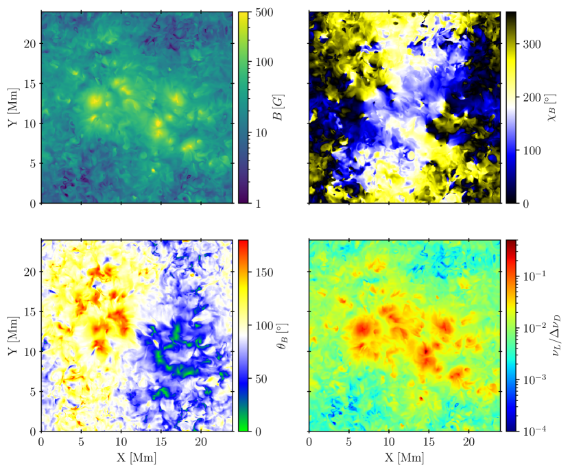
Figure 1: Top left: magnetic field strength. Top right: magnetic field azimuth. Bottom left: magnetic field inclination. Bottom right: ratio of the Larmor frequency over the thermal width of the line. All quantities are taken at the corrugated surface within the 3D model where the optical depth at the Ca i 4227 Å line-center is unity along the vertical line of sight.

The linear polarization of the Ca i 4227 Å line-center outside active regions is dominated by scattering processes and the Hanle effect. In this paper, we focus on theoretically investigating such spectral line polarization taking into account the effects of 3D radiative transfer. To this end, we consider a 3D model of an enhanced network region resulting from a radiation magneto-hydrodynamic simulation (see Carlsson et al., 2016) and calculate the Stokes profiles of the emergent radiation by applying the 3D radiative transfer code PORTA (Štěpán & Trujillo Bueno, 2013).

PORTA solves the non-LTE problem of the generation and transfer of spectral line polarization neglecting frequency correlations between the incoming and outgoing photons in the scattering events (see the relevant equations in section 7.2 of Landi Degl’Innocenti & Landolfi 2004). This complete frequency redistribution limit is suitable for estimating the scattering polarization at the line-center (e.g., Sampoorna et al., 2010) where the Hanle effect operates.

The upper-left panel in Figure 1 shows the magnetic field strength of the 3D snapshot model atmosphere at the heights where the line-center optical depth along the $\mu=1$ line of sight (LOS) is unity. The bottom left panel, showing the magnetic field inclination with respect to the local vertical, indicates that the 3D model presents two patches of opposite magnetic polarity separated by about 8 Mm, where the magnetic field strength reaches values larger than 200 G (see the upper left panel). The model’s magnetic field lines joining such two patches have a dominant azimuth (see the blue color in the upper right panel) and they reach chromospheric and coronal heights. Even at the relatively strong field locations of such patches the Zeeman splitting of the line’s upper level, as quantified by the Larmor frequency $\nu_{L}$, is smaller than the line’s Doppler width (see the lower right panel).

The dimensions of the 3D snapshot model atmosphere are $24\times 24\times 16.8\,\rm{Mm}^{3}$, going from $2.4\,\rm{Mm}$ below the average height of continuum optical depth unity to $14.4\,\rm{Mm}$ above. We point out that the atmospheric heights where the line-center optical depth of the Ca i 4227 Å line is unity lie several hundreds of kilometers below the model’s chromosphere-corona transition region. Accordingly, for the solution of the corresponding radiative transfer problem it was more than sufficient to restrict the vertical extension of the model from $0.1\,\rm{Mm}$ below the model’s visible surface to $2.5\,\rm{Mm}$ above.

Once the number density of Ca i is known at each spatial grid point, the Stokes profiles of the Ca i 4227 Å resonance line are calculated with PORTA using the two-level model atom approximation. This approximation is suitable because the level ${}^{1}{\rm P}_{1}^{\circ}$ of the Ca i atom, the upper level of the 4227 $\mathrm{\AA}$ line, is not radiatively coupled to any other lower level besides the ground level ${}^{1}{\rm S}_{0}$, the line’s lower level. The Einstein coefficient for spontaneous emission from the line’s upper level (angular momentum $J_{u}=1$ and Landé factor $g_{u}=1$) to the line’s lower level (angular momentum $J_{\ell}=0$) is $A_{ul}=2.18{\times}10^{8}\,\rm{s^{-1}}$. The rate of inelastic collisions with electrons from the upper level to the lower level ($C_{u\ell}$) was calculated following Seaton (1962) and the damping parameter was computed including the collisional broadening and the quadratic Stark effect Barklem et al. (1998). All these parameters, the background continuum quantities (opacity and emissivity) and the number density of Ca i atoms at each spatial grid point were computed with the RH code Uitenbroek (2001) using a more realistic atomic model with 20 Ca i levels and the ground level of Ca ii.

The critical magnetic field $B_{H}$ for the onset of the Hanle effect is 25 G ($B_{H}\approx 1.137\times 10^{-7}/(t_{\rm{life}}\,g_{u})$; $t_{\mathrm{life}}$ and $g_{u}$ being the lifetime of the upper level in seconds and its Landé factor, respectively). Because collisional depolarization is not significant for the core of this line, there is no collisional quenching (e.g., Alsina Ballester et al., 2018). Since the lower level has $J_{\ell}=0$, the scattering polarization in this line is solely due to the radiatively-induced atomic polarization of the upper level (i.e., to the population imbalances and quantum coherence between the magnetic sublevels of the line’s upper level with $J_{u}=1$).

3 Symmetry breaking by horizontal macroscopic velocities

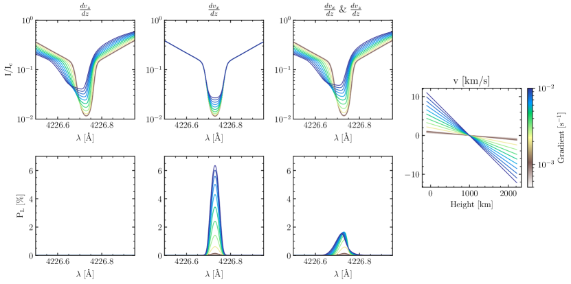
Figure 2: Emergent intensity (top row) and $P_{L}$ (bottom row) in the Ca i 4227 $\mathrm{\AA}$ line calculated in the FAL-C semi-empirical model for the disk-center LOS. First column: considering vertical gradients in the vertical velocity. Second column: vertical gradients in the horizontal velocity component (along the X axis). Third column: vertical gradients in both components. Each velocity component is defined by a linear $v_{x,z}(z)$ function decreasing with height with slopes between $5\cdot 10^{-4}$ and $10^{-2}~{}\rm{s^{-1}}$, fulfilling $v_{x,z}(1000)=0$ (right panel). Positive vertical velocities indicates that the plasma is moving towards the observer.

When the polarization of the spectral line radiation is ignored and one considers only the Stokes $I$ parameter, the relevant statistical equilibrium equations are those for the overall atomic level populations (e.g., Mihalas, 1978) and the radiation field is fully characterized by the mean intensity:

$$\bar{J^{0}_{0}}=\int d{\nu}\oint\frac{d\vec{\Omega}}{4\pi}{\phi\left(\nu\left[1-\frac{\vec{v}\cdot\vec{\Omega}}{c}\right]\right)}\,I_{\nu\vec{\Omega}}~{},$$ (1)

where $\phi$ is the Voigt absorption profile, $\nu$ the frequency, $\vec{v}$ the macroscopic plasma velocity and $\vec{\Omega}$ the propagation direction of the radiation beam. This direction is characterized by $\mu=\cos\theta$ (with $\theta$ the inclination of the ray with respect to the local vertical) and the azimuth $\chi$.

When scattering polarization is accounted for, the relevant statistical equilibrium equations are those for the density matrix elements $\rho^{K}_{Q}(J)$ for each atomic level with angular momentum $J$ (see Landi Degl’Innocenti & Landolfi, 2004, section 7.2). The mean intensity is no longer enough to characterize the radiation field, requiring the definition of the radiation field tensor $\bar{J}^{K}_{Q}$ with components:

$$\bar{J}^{2}_{0} =\frac{1}{2\sqrt{2}}\int d\nu\oint\frac{d\vec{\Omega}}{4\pi}{\phi\left(\nu\left[1-\frac{\vec{v}\cdot\vec{\Omega}}{c}\right]\right)}\Big{[}(3\mu^{2}-1)I_{\nu\vec{\Omega}}+3(\mu^{2}-1)Q_{\nu\vec{\Omega}}\Big{]},$$ (2a)

$${\rm Re}[{\bar{J}}^{2}_{1}] =\frac{\sqrt{3}}{2}\int d\nu\oint\frac{d\vec{\Omega}}{4\pi}{\phi\left(\nu\left[1-\frac{\vec{v}\cdot\vec{\Omega}}{c}\right]\right)}\sqrt{1-\mu^{2}}\Big{[}-\mu\cos\chi(I_{\nu\vec{\Omega}}+Q_{\nu\vec{\Omega}})+\sin\chi U_{\nu\vec{\Omega}}\Big{]},$$ (2b)

$${\rm Im}[{\bar{J}}^{2}_{1}] =\frac{\sqrt{3}}{2}\int d\nu\oint\frac{d\vec{\Omega}}{4\pi}{\phi\left(\nu\left[1-\frac{\vec{v}\cdot\vec{\Omega}}{c}\right]\right)}\sqrt{1-\mu^{2}}\Big{[}-\mu\sin\chi(I_{\nu\vec{\Omega}}+Q_{\nu\vec{\Omega}})-\cos\chi U_{\nu\vec{\Omega}}\Big{]},$$ (2c)

$${\rm Re}[{\bar{J}}^{2}_{2}] =\frac{\sqrt{3}}{4}\int d\nu\oint\frac{d\vec{\Omega}}{4\pi}\,{\phi\left(\nu\left[1-\frac{\vec{v}\cdot\vec{\Omega}}{c}\right]\right)}\bigg{[}\cos(2\chi)\Big{[}(1-\mu^{2})I_{\nu\vec{\Omega}}-(1+\mu^{2})Q_{\nu\vec{\Omega}}\Big{]}+2\sin(2\chi)\mu U_{\nu\vec{\Omega}}\bigg{]},$$ (2d)

$${\rm Im}[{\bar{J}}^{2}_{2}] =\frac{\sqrt{3}}{4}\int d\nu\oint\frac{d\vec{\Omega}}{4\pi}\,{\phi\left(\nu\left[1-\frac{\vec{v}\cdot\vec{\Omega}}{c}\right]\right)}\bigg{[}\sin(2\chi)\Big{[}(1-\mu^{2})I_{\nu\vec{\Omega}}-(1+\mu^{2})Q_{\nu\vec{\Omega}}\Big{]}-2\cos(2\chi)\mu U_{\nu\vec{\Omega}}\bigg{]},$$ (2e)

where $I_{\nu\vec{\Omega}}$, $Q_{\nu\vec{\Omega}}$, and $U_{\nu\vec{\Omega}}$ are the Stokes parameters for the given frequency ($\nu$) and direction ($\vec{\Omega}$). In these expressions the reference direction for positive $Q_{\nu\vec{\Omega}}$ is in the plane formed by $\vec{\Omega}$ and the local vertical. The $\bar{J}^{2}_{0}$ component quantifies the anisotropy of the incident radiation. The real and imaginary parts of the ${\bar{J}}^{2}_{1}$ and ${\bar{J}}^{2}_{2}$ components quantify the breaking of the axial symmetry of the incident radiation field with respect to the local vertical.

It is known that the spatial gradients of the vertical component of the macroscopic velocity can modify the values of the $\bar{J}^{2}_{0}$ anisotropy tensor and, therefore, the amplitude and shape of the scattering polarization profiles (see Carlin et al., 2012, 2013). Even more important is to note that the spatial gradients in the horizontal components of the macroscopic velocity break the axial symmetry of the incident radiation field Štěpán & Trujillo Bueno (2016); del Pino Alemán et al. (2018), even in an unmagnetized 1D model atmosphere. The ensuing non-zero values for the ${\bar{J}}^{2}_{1}$ and ${\bar{J}}^{2}_{2}$ tensors dramatically impact the $Q/I$ and $U/I$ signals, giving rise to forward scattering polarization without the need of inclined magnetic fields. In order to illustrate this, in Figure 2 we show the intensity and the total fractional linear polarization ($P_{L}=\sqrt{Q^{2}+U^{2}}/I$) profiles of the Ca i 4227 Å line for the disk-center LOS calculated in the semi-empirical model C of Fontenla et al. (1993), which is unmagnetized (hereafter, FAL-C model). We included macroscopic velocity fields with constant gradients in the vertical and horizontal components. Note that in a plane-parallel model atmosphere the only possible gradients are along the vertical direction. The right panel of Figure 2 shows the different macroscopic velocity gradients we have considered in the FAL-C model. Such academic velocity fields have zero velocity at the height where the optical depth is unity at the center of the Ca i 4227 Å line. We have opted for this curious choice to more easily emphasize the impact of the spatial gradients in the macroscopic velocity. When we only allow for the vertical component of the macroscopic velocity (first column), the intensity profiles are deformed due to different Doppler shifts at different atmospheric heights, and because the gradient is negative such deformation is more prominent in the blue part of the Stokes-$I$ profile. Clearly, the linear polarization at the solar disk center is zero, because the Doppler shifts caused by the vertical velocities are axially symmetric. However, there is a significant amount of forward-scattering polarization when we only consider the horizontal velocity component (second column). As expected, due to the azimuthally non-symmetric Doppler shifts, the stronger the gradient the larger the polarization signal. The line-center intensity becomes larger and flatter because of the broadening produced by the gradients in the horizontal velocity. When the gradients in both velocity components are included, the signal is much smaller and the shapes of the profiles are modified due to the impact of the Doppler shifts on the intensity profiles (third column).

4 An improved 1.5D approximation

The so-called 1.5D approximation for simplifying the numerical solution of non-LTE radiative transfer problems in 3D models of stellar atmospheres consists in neglecting the impact of horizontal radiative transfer on the excitation state of the atomic system. In other words, for each vertical column of the 3D model under consideration one solves the non-LTE radiative transfer problem as if such column was an independent 1D plane-parallel atmosphere.

To the best of our knowledge, the 1.5D approximation has always been applied neglecting the horizontal components of the model’s macroscopic velocity at each iterative step in the non-LTE radiative transfer calculation (e.g., Leenaarts et al., 2013a, b; Pereira et al., 2013; Carlin & Asensio Ramos, 2015; Carlin & Bianda, 2017). Under such circumstances, only the presence of magnetic fields inclined with respect to the local vertical can break the axial symmetry of the incident radiation field at each point within the model atmosphere. Consequently, only the Hanle effect due to the inclined magnetic fields can produce $Q/I$ and $U/I$ forward scattering (disk center) polarization signals. In other words, under such assumptions, the detection of scattering polarization at the solar disk-center implies the presence of an inclined magnetic field. While this is a valid conclusion when the radiation field that pumps the atomic system has axial symmetry around the local vertical (e.g., quiescent coronal filaments observed in the He i 10830 $\mathrm{\AA}$ multiplet, see Trujillo Bueno et al. 2002), it is not for spectral lines that originate within the inhomogeneous and dynamic plasma of the solar atmosphere itself.

The 1.5D approximation can never take into account the breaking of the axial symmetry of the pumping radiation field that results from the horizontal thermal and density inhomogeneities in the 3D model. Although this can only be accounted for via full 3D radiative transfer calculations, such as those reported below, the spatial gradients of the horizontal velocity components are an additional source of non-magnetic symmetry breaking that can be considered in the 1.5D approximation (the Doppler shift of these velocity components modify the symmetry properties of the incident radiation field; e.g., Figure 11 in del Pino Alemán et al. 2018, which shows the forward scattering polarization in the Sr i 4607 $\mathrm{\AA}$ line). By taking into account the horizontal components of the macroscopic velocity at each height for each individual column of the 3D model atmosphere we obtain forward scattering signals without the need of a magnetic field; i.e., we are able to account for the symmetry breaking that results from the vertical gradients of the horizontal component of the model’s macroscopic velocity.

To facilitate the identification of each particular radiative transfer solution we use the notation {$D$, $V_{h}$, $V_{z}$, $B$} where, for example, {1, 1, 1, 1} indicates the most realistic case of a full 3D solution ($D=1$) that takes into account the impact of the horizontal ($V_{h}=1$) and vertical ($V_{z}=1$) macroscopic velocities, and the Hanle effect produced by the model’s magnetic field ($B=1$), while {0, 0, 0, 0} refers to the 1.5D solution ($D=0$) ignoring the model’s horizontal ($V_{h}=0$) and vertical ($V_{z}=0$) macroscopic velocities and its magnetic field ($B=0$).

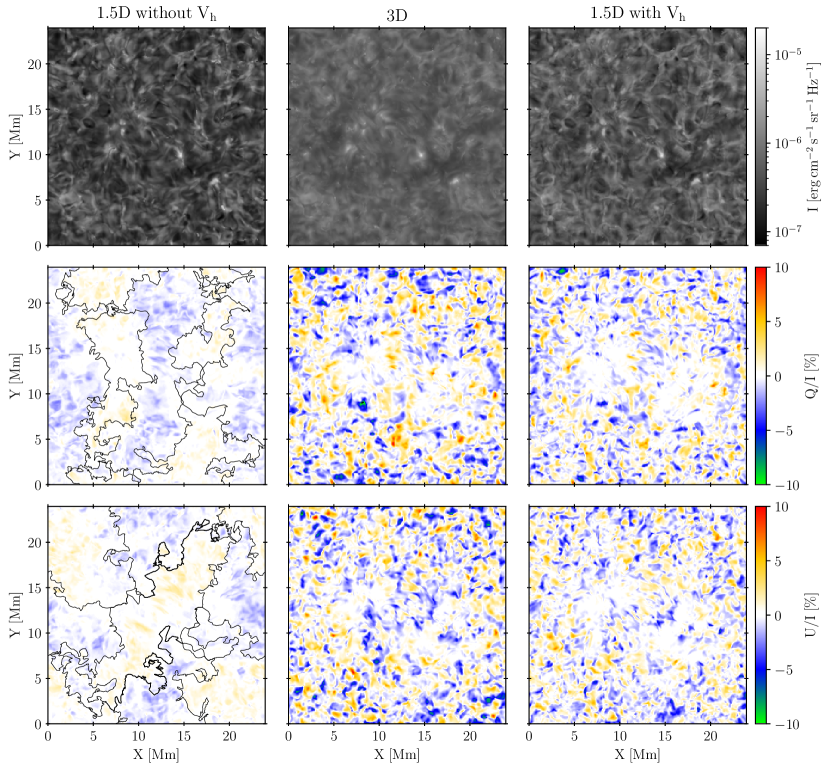
Figure 3: Values of the emergent Stokes $I$ (top row), $Q/I$ (middle row) and $U/I$ (bottom row) disk-center signals for the {0, 0, 1, 1} (left column), {1, 1, 1, 1} (middle column), and {0, 1, 1, 1} (right column) cases (see main text). The black contours show the positions where the model’s magnetic field azimuth has any of the following specific values at the heights where $\tau(\lambda_{P_{L}})=1$ (we recall that $\lambda_{P_{L}}$ is the wavelength at which $P_{L}$ has its maximum value). In the $Q/I$ panel such specific values are $\chi_{B}=45^{\circ}$, $135^{\circ}$, $225^{\circ}$, and $315^{\circ}$, while in the $U/I$ panel they are $\chi_{B}=0^{\circ}$, $90^{\circ}$, $180^{\circ}$, and $270^{\circ}$. We point out that for improving the visualization we have retained only the large-scale contours. The positive reference direction for Stokes $Q$ is along the Y-axis of the figures. The scale is saturated at $7\cdot 10^{-7}$ and $2\cdot 10^{-5}$ cgs for the intensity and at $\pm 10\%$ for $Q/I$ and $U/I$.

For each point of the field of view (FOV), Figure 3 shows the emergent Stokes $I$, $Q/I$, and $U/I$ disk-center signals at the wavelength $\lambda_{P_{L}}$ where the total linear polarization $P_{L}$ is maximum (hereafter, the $I$, $Q/I$, $U/I$ and $P_{L}$ signals). The various panels of the figure show such signals for (a) the 1.5D approximation neglecting the horizontal components of the macroscopic velocity (left column), (b) the full 3D solution (middle column), and (c) the 1.5D approximation taking into account the horizontal components of the velocity (right column). The self-consistent solutions have been obtained applying PORTA till reaching a maximum relative change smaller than $10^{-4}$ in the $\rho^{0}_{0}(J)$ density matrix elements. The emergent Stokes profiles have been calculated taking into account the Doppler shifts produced by the model’s macroscopic velocities along the LOS. Therefore, discrepancies in the calculated fractional polarization signals are solely due to the differences in the iteratively computed density matrix components $\rho^{K}_{Q}(J)$.

The left column of Figure 3 shows the $I$, $Q/I$, and $U/I$ signals for {0, 0, 1, 1}. The resulting $Q/I$ and $U/I$ disk-center signals are fully due to the Hanle effect caused by the model’s magnetic field, as there is no forward scattering polarization in the non-magnetic 1.5D case when the horizontal components of the macroscopic velocities are neglected (see the second panel of Figure 2). We see a $Q/I$ ($U/I$) pattern where the sign of $Q/I$ ($U/I$) is different inside and outside the contours indicated in the $Q/I$ ($U/I$) left panel of the figure. These contours in this $Q/I$ ($U/I$) panel indicate the points of the FOV where the model’s magnetic field azimuth (see Figure 1) is such that ${\rm cos}{2\chi_{B}}=0$ (${\rm sin}{2\chi_{B}}=0$), which is a factor appearing in an approximate equation for $Q/I$ ($U/I$) valid only for spectral lines in the saturation regime of the Hanle effect and whenever an inclined magnetic field is the only possible cause of symmetry breaking (e.g., Casini & Landi Degl’Innocenti, 2008; Trujillo Bueno, 2010; Carlin & Asensio Ramos, 2015).

The middle column of Figure 3 shows the emergent Stokes $I$, $Q/I$, and $U/I$ signals for the {1, 1, 1, 1} 3D solution, which accounts for all possible causes of symmetry breaking (magnetic and non-magnetic). In addition to the smoothing effect of horizontal radiative transfer, clearly seen in the intensity (top panel), the $Q/I$ and $U/I$ polarization patterns show more structure, with positive and negative signals covering relatively small patches all over the FOV, in contrast with the larger scale pattern of the {0, 0, 1, 1} solution (left column).

The right column of Figure 3 shows the emergent Stokes $I$, $Q/I$, and $U/I$ signals for the improved {0, 1, 1, 1} 1.5D solution, which includes the symmetry breaking caused by the vertical gradients of the horizontal components of the macroscopic plasma velocity. Interestingly, despite being a 1.5D solution, accounting for such non-magnetic symmetry breaking effects is sufficient to produce forward scattering polarization patterns qualitatively similar to those corresponding to the full {1, 1, 1, 1} 3D solution. However, there are some significant quantitative differences; e.g., while the spatially-averaged total linear polarization signal is $\langle P_{L}\rangle=2.3~{}\%$ in {1, 1, 1, 1}, it is $\langle P_{L}\rangle=1.8~{}\%$ in {0, 1, 1, 1}. This difference is due to the fact that only the full 3D solution can account for the symmetry breaking produced by the model’s horizontal inhomogeneities.

Figure 4: Pixel by pixel differences between the total linear polarization $P_{L}$ signal calculated without and with the model’s magnetic field, $P_{L}(B=0)-P_{L}$. Left panel: 1.5D approximation without $V_{h}$. Middle panel: full 3D calculation. Right panel: 1.5D approximation with $V_{h}$. The scale is saturated at $\pm 4$%.

Figure 4 quantifies the modification of the total linear polarization signals due to the Hanle effect –that is, it shows the differences in the $P_{L}$ signals when ignoring and taking into account the model’s magnetic field. The left panel shows the 1.5D approximation without horizontal velocities ({0, 0, 1, 0} vs {0, 0, 1, 1}), the middle panel the full 3D calculation ({1, 1, 1, 0} vs {1, 1, 1, 1}), and the right panel the 1.5D approximation with horizontal velocities ({0, 1, 1, 0} vs {0, 1, 1, 1}). As expected, the standard 1.5D approximation can only lead to the (generally wrong) conclusion that the Hanle effect produces forward scattering polarization (negative signs in the figure). However, the full 3D calculation shows that the Hanle effect tends to depolarize its non-magnetic forward scattering signals in the region where the model’s magnetic loops are concentrated (namely, the top-left bottom-right diagonal). A similar conclusion can be extracted from the right panel corresponding to the 1.5D calculation that includes the horizontal components of the velocity, although the Hanle depolarization is not as significant as in the correct 3D solution. Outside the region of the 3D model where the magnetic field is the strongest, it is equally likely to find pixels where the Hanle effect enhances or reduces the forward scattering polarization, in both the 3D and 1.5D solutions with horizontal velocities included. The impact of the Hanle effect on the linear scattering polarization depends on the spectral line under consideration (e.g., the review by Štěpán, 2015).

5 The impact of macroscopic velocity gradients on the scattering line polarization

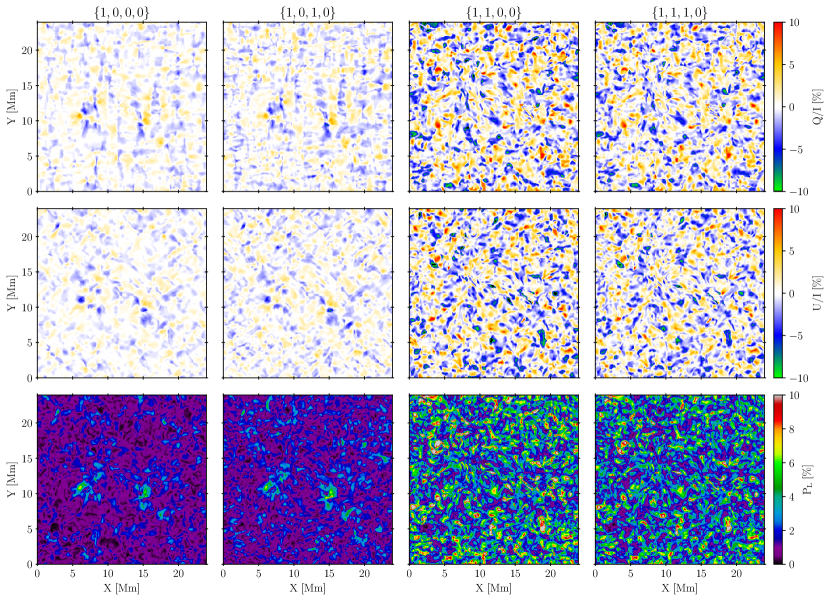
Figure 5: Non-magnetic $Q/I$ (top row), $U/I$ (middle row), and $P_{L}$ (bottom row) disk-center signals of the Ca i 4227 $\mathrm{\AA}$ line calculated by solving the 3D radiative transfer problem for the following cases: {1, 0, 0, 0} (first column), {1, 0, 1, 0} (second column), {1, 1, 0, 0} (third column), and {1, 1, 1, 0} (fourth column). The scales are saturated at $\pm 10~{}\%$. The positive reference direction for Stokes $Q$ is along the Y-axis of the figures.

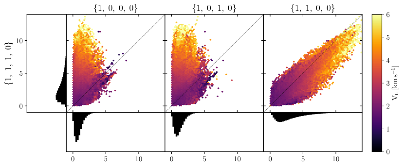
Figure 6: The $P_{L}$ signals (given in %) of the {1, 1, 1, 0} case versus those corresponding to the {1, 0, 0, 0} (left panel), {1, 0, 1, 0} (middle panel), and {1, 1, 0, 0} (right panel) solutions. The color scale indicates the modulus of the horizontal component of the model’s macroscopic velocities $V_{h}$ at the atmospheric heights where $\tau(\lambda_{P_{L}})=1$ in {1, 1, 1, 0}. In bins with more than one point the averaged $V_{h}$ is used. The diagonal dotted lines indicate where the points should be located in the case of a perfect correlation between the cases being compared. The black-colored areas at the left and at the bottom of the figure are 1D normalized histograms showing the distribution of $P_{L}$ values for each of the considered 3D non-magnetic solutions.

By means of full 3D radiative transfer calculations, in this section we study the impact of the gradients in the vertical and horizontal components of the model’s macroscopic velocities on the forward scattering polarization signals. Since we take into account the effects of horizontal radiative transfer, we are automatically accounting for the breaking of the axial symmetry of the pumping radiation field, with respect to the local vertical, produced by the horizontal thermal and density inhomogeneities in the 3D model atmosphere. In the 3D numerical experiments shown in this section we neglect the Hanle effect in order to isolate the non-magnetic sources of symmetry breaking. Every emergent Stokes signal shown in this section has been computed taking into account the Doppler shifts along the LOS and, therefore, any difference between the various cases is purely due to the impact of the velocity gradients on the density matrix elements $\rho^{K}_{Q}(J)$, and not due to LOS Doppler shifts.

To study the impact of the spatial gradients in the vertical component of the model’s macroscopic velocities we first compare the {1, 0, 0, 0} and {1, 0, 1, 0} cases. The axial symmetry breaking in the former is due solely to the model’s horizontal thermal and density inhomogeneities. In the latter, the gradients of the vertical component of the macroscopic velocity modify the {1, 0, 0, 0} forward scattering signals. Secondly, we consider the {1, 1, 0, 0} solution in order to reveal the dramatic impact caused by the spatial gradients of the horizontal component of the macroscopic velocities on the scattering polarization of the emergent spectral line radiation. Finally, we consider the general non-magnetic case (i.e., {1, 1, 1, 0}).

Figure 5 shows the $Q/I$, $U/I$, and $P_{L}$ signals for the above-mentioned cases, from left to right: {1, 0, 0, 0}, {1, 0, 1, 0}, {1, 1, 0, 0}, and {1, 1, 1, 0}. The first and second columns show very similar polarization patterns, thus indicating that the gradients of the vertical component of the macroscopic velocities slightly modify the forward scattering polarization signals ($\langle P_{L}\rangle\approx 1.0~{}\%$ in {1, 0, 0, 0} and $\langle P_{L}\rangle\approx 1.3~{}\%$ in {1, 0, 1, 0}). Both, the pattern and values of the polarization signals dramatically change when the gradients of the horizontal component of the macroscopic velocity are accounted for ({1, 1, 0, 0}, third column). In this case, the whole FOV is covered by small-scale sign-changing $Q/I$ and $U/I$ forward scattering signals, with $\langle P_{L}\rangle\approx 3.4~{}\%$. The full {1, 1, 1, 0} non-magnetic 3D solution (forth column) is qualitatively similar to the {1, 1, 0, 0} case (third column). The combined action of the vertical and horizontal velocity components gives a smaller average polarization, $\langle P_{L}\rangle\approx 3.0~{}\%$, compared with the {1, 1, 0, 0} case.

In order to relate the forward scattering signals with the plasma properties of the 3D model, we show in Figure 6 scatter plots comparing pixel-by-pixel the $P_{L}$ signals of the {1, 1, 1, 0} solution with the other three cases in Figure 5. The color table indicates the absolute value of the macroscopic horizontal velocities, $V_{h}=(v_{x}^{2}+v_{y}^{2})^{1/2}$, at $\tau_{\mu=1}=1$ and $\lambda_{P_{L}}$. Obviously, if the agreement (correlation) between two solutions were perfect, the points in the scatter plot would be located on the diagonal. From the left and middle panels, we see that the {1, 0, 0, 0} and {1, 0, 1, 0} clearly underestimate both the $P_{L}$ signals and range of variability ($P_{L}\lesssim 10\%$ in {1, 1, 1, 0} while $P_{L}\lesssim 5\%$ in {1, 0, 0, 0} and {1, 0, 1, 0}). The right panel, comparing {1, 1, 1, 0} and {1, 1, 0, 0}, shows a significant degree of correlation. This correlation means that we obtain similar $P_{L}$ signals from both solutions in the same pixels of the FOV. Interestingly, the vertical components of the macroscopic velocities slightly reduce the forward scattering signals generated by the axial symmetry breaking caused by the horizontal components of the macroscopic velocities. Furthermore, a careful attention to the color table of Figure 6 reveals that there is a correlation between horizontal velocities and the total linear polarization signals. Especially in the pixels of the FOV where there are large horizontal velocities we have strong linear polarization signals. We point out that the mere presence of horizontal velocities do not imply forward scattering signals, because spatial gradients are needed to break the axial symmetry. However, a 3D medium is highly complex and a correlation between $V_{h}$ and $P_{L}$ may occur because thermal, density and velocity field spatial distributions may be different in regions of the plasma with different levels of dynamical activity.

6 The impact of the Hanle effect

In §4 we already advanced some results regarding the impact of the Hanle effect on the scattering polarization at the center of the Ca i 4227$\mathrm{\AA}$ line while comparing the 1.5D and 3D approximations (see Figure 4). In this section we study in more detail the impact of the Hanle effect on the fractional linear polarization $Q/I$, $U/I$, and $P_{L}$ taking into account the effects of 3D radiative transfer.

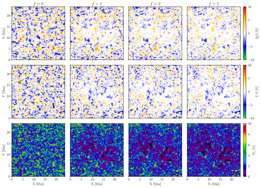
Figure 7: $Q/I$ (top row), $U/I$ (middle row), and $P_{L}$ (bottom row) signals of the emergent radiation in the Ca i 4227$\mathrm{\AA}$ line for the full 3D radiative transfer solutions. The different columns correspond to $f=0$ (first column), $f=1$ (second column), $f=2$ (third column), and $f=5$ (fourth column), with $f$ the scaling factor of the model’s magnetic field strength. The positive reference direction for Stokes $Q$ is along the Y-axis of the figures.

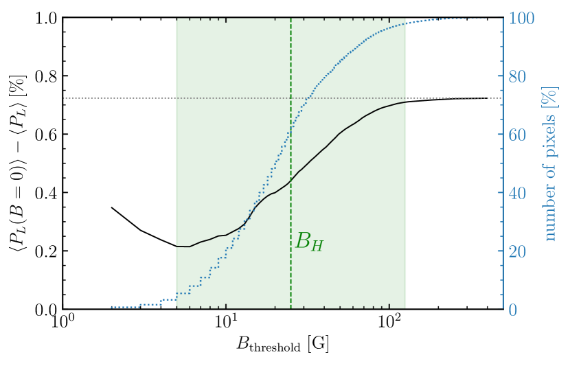
Figure 8: Black curve: average of the indicated $P_{L}$ signal differences considering the pixels where the magnetic field strength $B$ at the heigths where $\tau(\lambda_{P_{L}})=1$ is lower than $B_{\mathrm{threshold}}$. Blue curve: percentage of pixels in the FOV that fulfill the condition $B<B_{\mathrm{threshold}}$. The dashed vertical green line labelled $B_{H}$ indicates the critical Hanle field for the Ca i 4227$\mathrm{\AA}$ line. The shaded region goes from $0.2B_{H}$ to $5B_{H}$. The dotted horizontal black line shows the difference between the two averages considering all the pixels (i.e., the full FOV).

To this end, we solve the radiative transfer problem in the 3D model atmosphere, but multiplying the model’s magnetic field strength by a constant scaling factor $f$, namely, 0 (unmagnetized), 1 (true model’s magnetic field), 2, and 5 (Figure 7). We clearly appreciate that the Hanle effect tends to strongly depolarize the zero-field forward scattering signals in the region of the FOV with the largest magnetic field strengths (i.e., the region between the two opposite polarities in Figure 1). The average of the total linear polarization for the non-magnetic case is $\langle P_{L}(B=0)\rangle\approx 3.0\,\%$, while for the magnetic case ($f=1$) is $\langle P_{L}\rangle\approx 2.3\,\%$. However, outside such magnetic regions the role of the Hanle effect is less obvious. Considering only the $P_{L}$ signals in the pixels where $B<10$ G at the heights where $\tau(\lambda_{P_{L}})=1$ in the {1, 1, 1, 1} solution we obtain $\langle P_{L}(B=0)\rangle\approx 3.1\,\%$ and $\langle P_{L}\rangle\approx 2.8\,\%$. The $P_{L}$ signals of the emergent radiation are closer between the non-magnetic and magnetic solutions in the regions where the magnetic field is relatively weak. In order to study how the magnetic field strength modifies the linear polarization, we average the $P_{L}$ signals considering only the pixels in the FOV where $B<B_{\mathrm{threshold}}$ at the heights where $\tau(\lambda_{P_{L}})_{\mu=1}=1$ in {1, 1, 1, 1}. Figure 8 shows the difference $\langle P_{L}(B=0)\rangle-\langle P_{L}\rangle$ for several magnetic field thresholds. The difference starts to increase from $B_{\mathrm{threshold}}=5$ G and keep increasing with $B_{\mathrm{threshold}}$ up to $B_{\mathrm{threshold}}=125$ G. Note that, via the Hanle effect, the linear polarization is sensitive to magnetic field strengths between $0.2B_{H}$ and $5B_{H}$, which for the Ca i 4227 $\mathrm{\AA}$ line correspond to $5$ G and $125$ G, respectively. Therefore, we can conclude that most of the forward scattering polarization signals in the magnetic case are depolarized in regions where the line is sensitive to the Hanle effect.

On the other hand, the averaged $P_{L}$ signals for the $f=2$ and $f=5$ cases are $\langle P_{L}\rangle\approx 1.9\,\%$ and $\langle P_{L}\rangle\approx 1.7\,\%$, respectively. In these cases, the values are much more similar because for $f\geq 2$ the Ca i 4227 $\mathrm{\AA}$ line is practically in the Hanle saturation regime.

7 The impact of instrumental effects

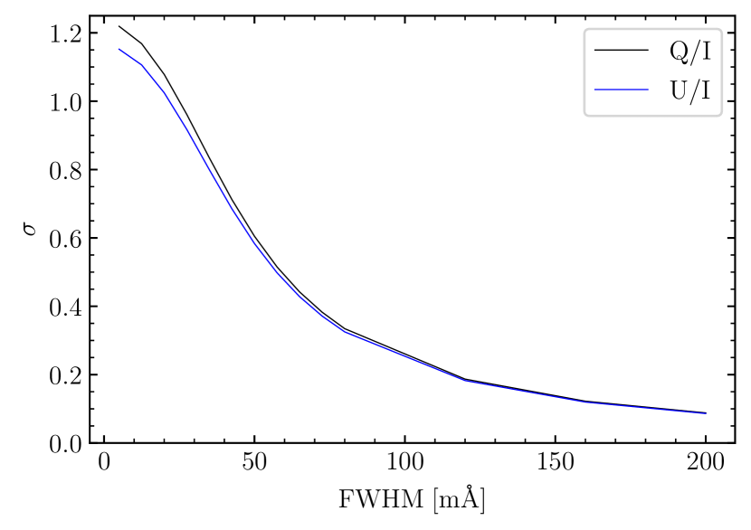
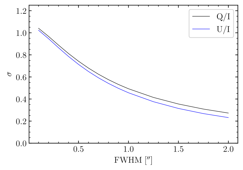
Figure 9: Left panel: sensitivity of the standard deviation of the $Q/I$ and $U/I$ spatial variations to the spectral resolution, assuming a seeing of 0$\farcs$5. Right panel: sensitivity of the standard deviation of the $Q/I$ and $U/I$ spatial variations to the seeing, assuming a spectral resolution of $\Delta\lambda=40\,\rm{m\AA}$.

One of the many scientific opportunities that the new generation of solar telescopes will provide is to measure, with unprecedented resolution, the polarization of chromospheric lines produced by anisotropic radiation pumping and the Hanle and Zeeman effects. In this respect, of particular interest are simulations showing what we may expect to detect using the ViSP instrument at DKIST. To this end, we have calculated the Stokes profiles of the Ca i 4227$\mathrm{\AA}$ line at the model’s disk-center taking into account the combined action of scattering processes and the Hanle and Zeeman effects, using the atomic density matrix elements iteratively computed with PORTA neglecting the Zeeman splittings.

The previous sections showed the Stokes signals of the Ca i 4227$\mathrm{\AA}$ line radiation calculated without accounting for any spatial and spectral degradation. In this section we show the impact that the finite spatial and spectral resolutions typical of real observations have on the synthetic Stokes profiles. To this end, we have applied a code developed by del Pino Alemán et al. (2018), which accounts for the following contributions:

1. The primary mirror diffraction and the atmospheric seeing, modeled applying the long-exposure approximation (see Fried & Cloud, 1966).

2. Diffraction in the spectral dimension, modeled by means of a convolution with a gaussian having full width at half maximum ${\rm FWHM}=\lambda_{0}/R$, where $R$ is the resolution power of the spectrograph and $\lambda_{0}$ the observed wavelength.

3. Finite width of the spectrograph slit. For each position of the FOV covered by the slit, the emergent Stokes profiles for all the points across its width are added together.

4. Finite pixel size. The Stokes profiles of the emergent radiation for all the points in the surface of the 3D model inside the projection of each CCD pixel over the surface are added together.

5. We add some noise by adding random values to $Q$, $U$ and $V$ following a gaussian distribution with a given standard deviation $\sigma_{Q}$, $\sigma_{U}$, and $\sigma_{V}$, respectively.

The left panel of Figure 9 shows the change of the standard deviation of the $Q/I$ and $U/I$ forward scattering signals for different spectral resolutions at a fixed 0$\farcs$5 spatial resolution. The standard deviation of the $Q/I$ and $U/I$ spatial variations is reduced by a factor two for a spectral resolution of 50 m$\mathrm{\AA}$. Clearly, a spectral resolution significantly better than 100 $\rm{m\AA}$ is needed to detect the spatial fluctuations of the polarization signals.

Complementary information is provided in the right panel of Figure 9, which shows the standard deviation of the $Q/I$ and $U/I$ disk-center signals for different spatial resolutions at a fixed 40 $\rm{m\AA}$ spectral resolution. The panel shows that for a seeing of $1\arcsec$ the standard deviation of the $Q/I$ and $U/I$ spatial variations is reduced by a factor two. A spatial resolution better than $2\arcsec$ is essential to detect spatial variations in the $Q/I$ and $U/I$ disk-center signals.

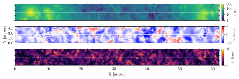
Figure 10: Magnetic field strength (top panel), vertical velocity $V_{z}$ (middle panel), and horizontal velocity $\sqrt{V_{x}^{2}+V_{y}^{2}}$ (bottom panel) at the corrugated surface within the 3D model where $\tau(\lambda_{P_{L}})=1$. Each panel shows the region around the spectrograph slit indicated with the white line.

The white line in Figure 10 visualizes the spectrograph’s slit covering $62\arcsec$ on the surface of the 3D model. As seen in the figure, we have oriented the slit so as to cross a few patches of magnetic flux concentrations having field strengths exceeding $100\,\rm{G}$ (see the upper panel in Figure 10). We can also find significant (several km/s) macroscopic velocities, both vertical and horizontal, along the spatial direction of the spectrograph’s slit at the chromospheric heights where the optical depth at the wavelength $\lambda_{P_{L}}$ is unity (see middle and bottom panels in Figure 10).

Figure 11: Simulation of slit spectropolarimetric observations with ViSP at DKIST. Top: for an exposure time of $5\,\rm{s}$, which implies a noise PDF of $\sigma=10^{-4}$. Bottom: for an exposure time of $490\,\rm{s}$, which implies a noise PDF of $\sigma=10^{-5}$. In each pair of panels (for $Q/I$, $U/I$ or $V/I$) the right one shows the non-magnetic case, while the left one includes the impact of the model’s magnetic field through the Hanle and Zeeman effects. The reference direction for $Q>0$ is along the spatial direction of the slit. The color tables are saturated at $\pm 1\%$.

The ViSP instrument offers several configurations. We have selected the second arm with a spatial sampling of $0\farcs 0242$ and the $0\farcs 2142$ wide slit, with a spectral sampling of $8.4\,\rm{m\AA}$. With this set-up the resolution power is $R=70\,000$. We characterize the noise in the polarization quantities with the standard deviation ($\sigma_{QUV}$) of a gaussian probability distribution function (PDF) given in units of the continuum intensity. The width of the noise distribution depends on the exposure time; thus, we have chosen the following two: $t=5\,\rm{s}$ ($\sigma_{QUV}=4.5\cdot 10^{-4}$) and $t=490\,\rm{s}$ ($\sigma=4.5\cdot 10^{-5}$).

The spatial resolution is typically limited by the atmospheric seeing, which we assume to be $0\farcs 5$. Since the pixel size is below the spatial resolution, we bin 10 pixels along the slit increasing the signal to noise ratio (SNR). Consequently, our simulated observations have a spatial and spectral resolution of $0\farcs 5$ and $60\,\rm{m\AA}$, respectively, and the noise PDF turns out to be $\sigma_{QUV}=10^{-4}$ for $t=5\,\rm{s}$ and $\sigma_{QUV}=10^{-5}$ for $t=490\,\rm{s}$.

Figure 11 shows the $Q/I$, $U/I$ and $V/I$ profiles, at each point along the slit, corresponding to the above-mentioned ViSP instrumental setup and for $t=5\,\rm{s}$ (top panel) and $t=490\,\rm{s}$ (bottom panel) exposure times. Each panel in the figure shows three pairs of plots, one for each fractional Stokes parameter, and with each pair showing the cases where we take into account (left) or neglect (right) the model’s magnetic field. As expected, the $V/I$ Zeeman signals are very significant where we have the largest longitudinal magnetic field strengths, showing signals above 1% (see the left side of the right column in Figure 11). In such regions the Hanle effect tends to depolarize the non-magnetic linear polarization signals (see left and middle columns in Figure 11). Outside such “strong field” patches the model’s magnetic field is too weak so as to produce a very clear impact on the $Q/I$ and $U/I$ signals, neither through the Hanle nor the Zeeman effects. We find that the linear scattering polarization signals are dominated by the breaking of the axial symmetry produced by the spatial gradients of the horizontal components of the model’s macroscopic velocities. Moreover, in the pixels where the magnetic field strength is around the critical Hanle field ($B_{\rm H}={25\,\mathrm{G}}$) the Hanle effect significantly modifies the scattering polarization signals. For example, at position $42\arcsec$ along the slit we see a non-magnetic positive $Q/I$ signal of about 1% (left side in left panel). This is considerably reduced by a $\sim 75$ G magnetic field (right side in left panel), which is not sufficient to generate significant circular polarization via the Zeeman effect.

With its 4 meter mirror the collecting surface of DKIST is significantly larger than in the previous generation of solar telescopes, such as the 1.5 meter mirror of the GREGOR telescope operating at the Observatorio del Teide (Canary Islands, Spain). The Zürich Imaging Polarimeter (ZIMPOL) attached to GREGOR could be used for doing spectropolarimetric observations of the Ca i 4227 Å line with a spatial and spectral sampling of $0\farcs 33$ and $7.9\,\rm{m\AA}$, respectively, giving a spectral resolution power of $200\,000$ with the $0\farcs 3$ slit. We can expect a noise PDF of about $\sigma_{QUV}=10^{-4}$ for $15\,\rm{min}$ exposure time. Reaching $\sigma_{QUV}=4\cdot 10^{-5}$ with ZIMPOL at GREGOR would require 2 hours of exposure time. Clearly, the large collecting area of DKIST is a big advantage, although it remains to be seen if such a high polarimetric sensitivity can be reached without the very fast polarization modulation that is possible with the ZIMPOL instrument.

Figure 12: Simulation of slit spectropolarimetric observations with ViSP at the diffraction limit of the DKIST telescope. The spatial resolution is $0\farcs 0398$ and the spectral resolution $14.6\,\rm{m\AA}$. The reference direction for $Q>0$ is along the spatial direction of the slit.

When observing at the diffraction limit of a telescope the SNR is independent of its aperture (e.g., Landi Degl’Innocenti, 2013). It is of interest to consider now the case of spectropolarimetric observations with ViSP at the spatial resolution limit of DKIST ($0\farcs 026$). Obviously, matching this resolution is only possible if the adaptive optics (AO) system can correct at this precision during the whole integration time. The minimum spatial sampling can be achieved with arm 3, $0\farcs 0199$ covering $51\,\rm{arcsec}$ along the slit, giving a resolution of $0\farcs 0398$. With the narrowest slit ($0\farcs 0284$), we get a spectral sampling of $7.3\,\rm{m\AA}$ and a spectral resolution of $\Delta\lambda=14.6\,\rm{m\AA}$. The top panels of Figure 12 show the simulated observation corresponding to this configuration, with an exposure time of $7$ second resulting in a noise PDF with $\sigma_{QUV}=10^{-3}$. The bottom panels show the case for an exposure time of $2.7\,\mathrm{min}$ resulting in a noise PDF with $\sigma_{QUV}=2\cdot 10^{-4}$. Clearly, achieving a high enough SNR is important for a clear detection and quantification of the weakest polarization signals, along with their spatial variability. We point out that the temporal evolution of the chromospheric plasma has not been considered here, because full 3D radiative transfer calculations are computationally costly; the signals and spatial variations shown in the figure would decrease as the exposure time of the simulated observation increases.

8 Summary and conclusions

We have carried out a detailed 3D radiative transfer investigation of the linear polarization signals produced by forward scattering processes in the core of the Ca i 4227 Å line, sensitive to chromospheric magnetic fields via the Hanle effect. To this end, we have applied PORTA, a 3D radiative transfer code for modeling the intensity and polarization of spectral lines with massively parallel computers (Štěpán & Trujillo Bueno, 2013). The solar model atmosphere used is a 3D snapshot model resulting from a radiation magneto-hydrodynamic simulation by Carlsson et al. (2016), which is representative of an enhanced-network region.

We show that the line’s Doppler shifts resulting from the spatial gradients of the horizontal components of the plasma macroscopic velocities break the axial symmetry of the radiation field that illuminates each point within the model chromosphere, to the extent that they produce sizable forward scattering polarization in the core of the Ca i 4227 Å line without the need of any magnetic field (see Figure 5). The spatial gradients of the vertical components of the macroscopic velocities must also be taken into account because the ensuing line’s Doppler shifts modify the radiation field anisotropy and the scattering polarization signals. Interestingly, the correlation between $V_{h}$ and $P_{L}$ seen in Figure 6 suggests that regions of the solar chromosphere showing large horizontal velocities may also show strong forward-scattering polarization signals in the Ca i 4227 Å line.

The Hanle effect caused by the model’s magnetic field tends to depolarize the $Q/I$ and $U/I$ disk-center signals at the locations of the field of view where $5$ G $<B<125$ G in the lower chromosphere (see Figures 7 and 8). However, in the regions where the magnetic field is weaker, the Hanle effect just modifies the emergent linear polarization without a dominant tendency. The Ca i 4227 $\mathrm{\AA}$ line is in the Hanle saturation regime for $B>125$ G. In such regime, the linear polarization is no longer sensitive to the magnetic field strength, but only to its orientation.

The 1.5D approximation, when applied retaining only the vertical components of the plasma macroscopic velocities, is unsuitable for modeling the forward scattering polarization of this line, because it leads to the wrong conclusion that detection of polarization implies the presence of inclined magnetic fields. We have accounted for the symmetry breaking produced by the horizontal components of the plasma macroscopic velocities in the 1.5D approximation, which provides results in qualitative agreement with the full 3D calculations (see Figure 3). Full 3D radiative transfer is however needed for an accurate quantification of the scattering polarization signals.

Finally, our simulations of the scattering polarization signals of the Ca i 4227 Å line taking into account the degradation of instrumental effects show that a spectral resolution and a spatial resolution better than 100 m$\mathrm{\AA}$ and 2$\arcsec$ are essential to detect spatial variations of the disk-center polarization signals (see Figure 9). The Visible Spectro-Polarimeter (ViSP) at the DKIST achieves such requirements with a very high SNR in few seconds. We have simulated spectropolarimetric observations with the ViSP with a spatial resolution limited by seeing (see Figure 11). Considering an integration time of 5 seconds, we are able to detect the spatial variations of the strongest scattering polarization signals. As we increase the exposure time, the SNR is larger and we can then appreciate much better the rich spatial variability on the forward-scattering polarization signals. To observe at the spatial resolution limit of the telescope (see Figure 12) we would need at least 2 minutes of exposure time to detect the spatial variations with sufficient SNR. Finally, it is important to note that we have not considered the temporal evolution of the chromospheric plasma; therefore, as we increase the exposure time the signals would decrease due to signal cancellations and the spatial variations would be more difficult to detect.

Clearly, a reliable modeling of the linear polarization produced by scattering processes in the Ca i 4227 Å chromospheric line requires taking into account all the causes that may break the axial symmetry of the pumping radiation field, both magnetic and non-magnetic. In this paper we have taken all such symmetry breaking causes into account showing how the line’s scattering polarization is sensitive to the magnetic, thermal and dynamic structure of the lower solar atmosphere. The radiative transfer tools (see the public repository of PORTA at https://gitlab.com/polmag/PORTA) needed for this type of modeling are at the disposal of the astrophysical community for validating or refuting the 3D models of the solar chromosphere, by means of contrasting the calculated Stokes profiles with the unprecedented spectropolarimetric observations that the new generation of solar telescopes will hopefully provide.

References

- Alsina Ballester et al. (2018) Alsina Ballester, E., Belluzzi, L., & Trujillo Bueno, J. 2018, ApJ, 854, 150, doi: 10.3847/1538-4357/aa978a
- Anusha et al. (2011) Anusha, L. S., Nagendra, K. N., Bianda, M., et al. 2011, ApJ, 737, 95, doi: 10.1088/0004-637X/737/2/95
- Auer et al. (1980) Auer, L. H., Rees, D. E., & Stenflo, J. O. 1980, A&A, 88, 302
- Barklem et al. (1998) Barklem, P. S., Anstee, S. D., & O’Mara, B. J. 1998, Publications of the Astronomical Society of Australia, 15, 336, doi: 10.1071/AS98336
- Bommier & Landi Degl’Innocenti (1996) Bommier, V., & Landi Degl’Innocenti, E. 1996, Sol. Phys., 164, 117, doi: 10.1007/BF00146628
- Carlin & Asensio Ramos (2015) Carlin, E. S., & Asensio Ramos, A. 2015, ApJ, 801, 16, doi: 10.1088/0004-637X/801/1/16
- Carlin et al. (2013) Carlin, E. S., Asensio Ramos, A., & Trujillo Bueno, J. 2013, ApJ, 764, 40, doi: 10.1088/0004-637X/764/1/40
- Carlin & Bianda (2017) Carlin, E. S., & Bianda, M. 2017, ApJ, 843, 64, doi: 10.3847/1538-4357/aa7800
- Carlin et al. (2012) Carlin, E. S., Manso Sainz, R., Asensio Ramos, A., & Trujillo Bueno, J. 2012, ApJ, 751, 5, doi: 10.1088/0004-637X/751/1/5
- Carlsson et al. (2016) Carlsson, M., Hansteen, V. H., Gudiksen, B. V., Leenaarts, J., & De Pontieu, B. 2016, A&A, 585, A4, doi: 10.1051/0004-6361/201527226
- Casini & Landi Degl’Innocenti (2008) Casini, R., & Landi Degl’Innocenti, E. 2008, Astrophysical Plasmas, ed. T. Fujimoto & A. Iwamae, Vol. 44, 247, doi: 10.1007/978-3-540-73587-8_12
- del Pino Alemán et al. (2018) del Pino Alemán, T., Trujillo Bueno, J., Štěpán, J., & Shchukina, N. 2018, ApJ, 863, 164, doi: 10.3847/1538-4357/aaceab
- Dumont et al. (1973) Dumont, S., Pecker, J.-C., & Omont, A. 1973, Sol. Phys., 28, 271, doi: 10.1007/BF00152298
- Faurobert (1988) Faurobert, M. 1988, A&A, 194, 268
- Faurobert-Scholl (1992) Faurobert-Scholl, M. 1992, A&A, 258, 521
- Fontenla et al. (1993) Fontenla, J. M., Avrett, E. H., & Loeser, R. 1993, ApJ, 406, 319, doi: 10.1086/172443
- Fried & Cloud (1966) Fried, D. L., & Cloud, J. D. 1966, Journal of the Optical Society of America (1917-1983), 56, 1667
- Gandorfer (2002) Gandorfer, A. 2002, The Second Solar Spectrum: A high spectral resolution polarimetric survey of scattering polarization at the solar limb in graphical representation. Volume II: 3910 Å to 4630 Å
- Landi Degl’Innocenti (2013) Landi Degl’Innocenti, E. 2013, Memorie della Societa Astronomica Italiana, 84, 391
- Landi Degl’Innocenti & Landolfi (2004) Landi Degl’Innocenti, E., & Landolfi, M., eds. 2004, Astrophysics and Space Science Library, Vol. 307, Polarization in Spectral Lines, doi: 10.1007/1-4020-2415-0
- Leenaarts et al. (2013a) Leenaarts, J., Pereira, T. M. D., Carlsson, M., Uitenbroek, H., & De Pontieu, B. 2013a, ApJ, 772, 90, doi: 10.1088/0004-637X/772/2/90
- Leenaarts et al. (2013b) —. 2013b, ApJ, 772, 89, doi: 10.1088/0004-637X/772/2/89
- Manso Sainz & Trujillo Bueno (2011) Manso Sainz, R., & Trujillo Bueno, J. 2011, ApJ, 743, 12, doi: 10.1088/0004-637X/743/1/12
- Megha et al. (2019) Megha, A., Sampoorna, M., Nagendra, K. N., Anusha, L. S., & Sankarasubramanian, K. 2019, ApJ, 879, 48, doi: 10.3847/1538-4357/ab24cc
- Mihalas (1978) Mihalas, D. 1978, Stellar atmospheres
- Pereira et al. (2013) Pereira, T. M. D., Leenaarts, J., De Pontieu, B., Carlsson, M., & Uitenbroek, H. 2013, ApJ, 778, 143, doi: 10.1088/0004-637X/778/2/143
- Rees & Saliba (1982) Rees, D. E., & Saliba, G. J. 1982, A&A, 115, 1
- Rimmele et al. (2020) Rimmele, T. R., et al. 2020, Solar Physics, in press
- Sampoorna & Nagendra (2015) Sampoorna, M., & Nagendra, K. N. 2015, ApJ, 812, 28, doi: 10.1088/0004-637X/812/1/28
- Sampoorna et al. (2010) Sampoorna, M., Trujillo Bueno, J., & Landi Degl’Innocenti, E. 2010, ApJ, 722, 1269, doi: 10.1088/0004-637X/722/2/1269
- Seaton (1962) Seaton, M. J. 1962, The Observatory, 82, 111
- Supriya et al. (2014) Supriya, H. D., Smitha, H. N., Nagendra, K. N., et al. 2014, ApJ, 793, 42, doi: 10.1088/0004-637X/793/1/42
- Trujillo Bueno (2001) Trujillo Bueno, J. 2001, in Astronomical Society of the Pacific Conference Series, Vol. 236, Advanced Solar Polarimetry – Theory, Observation, and Instrumentation, ed. M. Sigwarth, 161. https://arxiv.org/abs/astro-ph/0202328
- Trujillo Bueno (2010) Trujillo Bueno, J. 2010, Astrophysics and Space Science Proceedings, 19, 118, doi: 10.1007/978-3-642-02859-5_9
- Trujillo Bueno et al. (2002) Trujillo Bueno, J., Landi Degl’Innocenti, E., Collados, M., Merenda, L., & Manso Sainz, R. 2002, Nature, 415, 403. https://arxiv.org/abs/astro-ph/0201409
- Uitenbroek (2001) Uitenbroek, H. 2001, ApJ, 557, 389, doi: 10.1086/321659
- Štěpán (2015) Štěpán, J. 2015, in IAU Symposium, Vol. 305, Polarimetry, ed. K. N. Nagendra, S. Bagnulo, R. Centeno, & M. Jesús Martínez González, 360–367, doi: 10.1017/S1743921315005050
- Štěpán & Trujillo Bueno (2013) Štěpán, J., & Trujillo Bueno, J. 2013, A&A, 557, A143, doi: 10.1051/0004-6361/201321742
- Štěpán & Trujillo Bueno (2016) —. 2016, ApJ, 826, L10, doi: 10.347/2041-8205/826/1/L10