Trace Ratio Optimization with an Application to Multi-view Learning

Abstract.

A trace ratio optimization problem over the Stiefel manifold is investigated from the perspectives of both theory and numerical computations. At least three special cases of the problem have arisen from Fisher’s linear discriminant analysis, canonical correlation analysis, and unbalanced Procrustes problem, respectively. Necessary conditions in the form of nonlinear eigenvalue problem with eigenvector dependency are established and a numerical method based on the self-consistent field (SCF) iteration is designed and proved to be always convergent. As an application to multi-view subspace learning, a new framework and its instantiated concrete models are proposed and demonstrated on real world data sets. Numerical results show that the efficiency of the proposed numerical methods and effectiveness of the new multi-view subspace learning models.

1. Introduction

We are concerned with the following trace ratio maximization problem

(1.1a) $$\max_{X^{\operatorname{T}}X=I_{k}}f_{\theta}(X),$$

where $$1\leq k<n I_{k} k\times k$$, is the identity matrix, and

(1.1b) $$f_{\theta}(X)=\frac{\operatorname{trace}(X^{\operatorname{T}}AX+X^{\operatorname{T}}D)}{[\operatorname{trace}(X^{\operatorname{T}}BX)]^{\theta}},$$

$A,\,B\in\mathbb{R}^{n\times n}$ are symmetric and $B$ is positive semi-definite with $\operatorname{rank}(B)>n-k$, $D\in\mathbb{R}^{n\times k}$, matrix variable $X\in\mathbb{R}^{n\times k}$, and parameter $0\leq\theta\leq 1$. The condition that $\operatorname{rank}(B)>n-k$ ensures the denominator of $f_{\theta}(X)$ is always positive for any $X$ such that $X^{\operatorname{T}}X=I_{k}$.

Problem (1.1) is a maximization problem on the Stiefel manifold [1]:

$$\mathbb{O}^{n\times k}=\{X\in\mathbb{R}^{n\times k}\,:\,X^{\operatorname{T}}X=I_{k}\}.$$

A seemingly more general case than (1.1) is to maximize

(1.2) $$\frac{\operatorname{trace}(X^{\operatorname{T}}AX+X^{\operatorname{T}}D)+c}{[\operatorname{trace}(X^{\operatorname{T}}BX)]^{\theta}}=\frac{\operatorname{trace}(X^{\operatorname{T}}[A+c/k)I_{n}]X+X^{\operatorname{T}}D)}{[\operatorname{trace}(X^{\operatorname{T}}BX)]^{\theta}}$$

over $X\in\mathbb{O}^{n\times k}$, but it is actually a special case of (1.1) due to the reformulation on the right-hand side of (1.2), where $c\in\mathbb{R}$ is a scalar constant.

1.1. Previous Work

There are three special cases arising from data science that have been fairly well studied in the last decades.

The first special case is with $D=0$ and $\theta=1$:

(1.3) $$\max_{X\in\mathbb{O}^{n\times k}}\frac{\operatorname{trace}(X^{\operatorname{T}}AX)}{\operatorname{trace}(X^{\operatorname{T}}BX)}$$

arising from Fisher’s linear discriminant analysis [31, 46, 47] in the setting of supervised learning. In [31], (1.3) is converted into a zero-finding problem

$$\mbox{solve}\,\,\eta(\rho)=0\quad\mbox{with}\quad\eta(\rho):=\max_{X\in\mathbb{O}^{n\times k}}\operatorname{trace}(X^{\operatorname{T}}(A-\rho B)X).$$

It is proved there that $\eta(\rho)$ is a non-increasing function of $\rho$ and has a unique zero in the generic case, and the Newton method is applied to find the zero [31]. This idea of such conversion can be traced back to [10] in 1967 for fractional programming. In [46, 47], however, (1.3) is treated as a maximization problem on the Stiefel manifold $\mathbb{O}^{n\times k}$. Their major results are as follows. The KKT condition of (1.3) with respect to the Stiefel manifold is a nonlinear eigenvalue problem with eigenvector dependency (NEPv) [5]:

(1.4) $$H(X)X=X\Lambda,$$

where $H(X)\in\mathbb{R}^{n\times n}$ is a matrix-valued function of $X\in\mathbb{O}^{n\times k}$ and symmetric, and $\Lambda\in\mathbb{R}^{k\times k}$ is not really an unknown since it can be expressed as $\Lambda=X^{\operatorname{T}}H(X)X\in\mathbb{R}^{k\times k}$. NEPv (1.4) is then solved by the so-called self-consistent field (SCF) iteration

(1.5) iterate $$H(X_{i-1})X_{i}=X_{i}\Lambda_{i-1} X_{0}$$, given

where $X_{i}$ is an orthonormal basis matrix associated with the $k$ largest eigenvalues of $H(X_{i-1})$. It is noted that SCF has been widely used in electronic structure calculations for decades [28, 36]. Remarkably, it is proved in [46, 47] that (i) problem (1.3) has no local maximizer but global ones, (ii) the SCF iteration is monotonically convergent in terms of the objective value, and the iterates $X_{i}$ globally converge to a maximizer in the metric on the Grassmann manifold $\mathscr{G}_{k}(\mathbb{R}^{n})$ (the collection of all $k$-dimensional subspaces of $\mathbb{R}^{n}$), and (iii) the convergence is locally quadratic in the generic case. A shorter proof of the local quadratic convergence can be found in [5].

The second special case is with $A=0$ and $\theta=1/2$:

(1.6) $$\max_{X\in\mathbb{O}^{n\times k}}\frac{\operatorname{trace}(X^{\operatorname{T}}D)}{\sqrt{\operatorname{trace}(X^{\operatorname{T}}BX)}},$$

arising from orthogonal canonical correlation analysis (OCCA) [45] as the kernel of an alternating iterative scheme. The major results established in [45] for (1.6) can be summarized as follows. The KKT condition of (1.6) with respect to the Stiefel manifold $\mathbb{O}^{n\times k}$ does not exactly take the form of an NEPv but can be equivalently converted into one like (1.4). The latter can again be solved by SCF iteration (1.5) followed by a post-processing on $X_{i}$. The method is monotonically convergent in the objective value and the iterates $X_{i}$ globally converge to a critical point that satisfies an established necessary condition for a global minimizer.

The third special case is with $B=I_{n}$ and $\theta=0$:

(1.7) $$\max_{X\in\mathbb{O}^{n\times k}}{\operatorname{trace}(X^{\operatorname{T}}AX+X^{\operatorname{T}}D)}.$$

This is a rather fundamental problem in numerical linear algebra, optimization, and applied statistics, among others, and is commonly referred to as the unbalanced Procrustes problem [7, 12, 13, 16, 18, 48, 49]. In particular, the following least-squared minimization

(1.8) $$\min_{X\in{\mathbb{O}}^{n\times k}}\|CX-B\|_{\operatorname{F}}^{2}$$

can be reformulated into (1.7) with $A=-C^{\operatorname{T}}C$ and $D=C^{\operatorname{T}}B/2$. Both (1.7) and (1.8) can be found in many real world applications including the orthogonal least squares regression (OLSR) for feature extraction [50, 32], the multidimensional similarity structure analysis (SSA) [4, Chapter 19], and the MAXBET problem [14, 27] in the canonical correlation analysis. A recent work [48] turns (1.8) into an equivalent NEPv that is solved by an SCF iteration in the form (1.5), among others.

There are some fundamental differences among these special cases (1.3), (1.6), and (1.7), and their associated NEPv [46, 47, 45, 48]. Three major differences are as follows.

• If $X_{\operatorname*{opt}}$ is a maximizer of (1.3) then so is $X_{\operatorname*{opt}}Q$ for any $Q\in\mathbb{O}^{k\times k}$. In this sense any maximizer of (1.3) is a representative of a class of maximizers. But that is not the case for (1.6), namely for a maximizer $X_{\operatorname*{opt}}$ of (1.6), $X_{\operatorname*{opt}}Q$ for a generic $Q\in\mathbb{R}^{k\times k}$ is most likely not another maximizer.

• Problem (1.3) has no local maximizer but global ones, whereas (1.6) and (1.7) are numerically demonstrated to have local maximizers.

• NEPv (1.4) for (1.3) admits an orthogonal-invariance property: $H(XQ)=H(X)$ for any $Q\in\mathbb{O}^{k\times k}$, while the ones associated with (1.6) and (1.7) do not have this property.

1.2. Contributions and the Organization of This Paper

In this paper, our goal is to thoroughly investigate problem (1.1) as a maximization problem on the Stiefel manifold $\mathbb{O}^{n\times k}$ in both theory and numerical computation. Our major contributions are as follows: 1) We turn the KKT condition of (1.1) with respect to the Stiefel manifold equivalently into an NEPv; 2) We establish crucial necessary conditions, beyond the KKT condition, of local and global maximizers in terms of the extreme eigenvalues of the NEPv; 3) We completely characterize the role of $D$ in how precisely it determines maximizers, which is important because when $D=0$, any maximizer represents a class of many associated with an element of the Grassmann manifold $\mathscr{G}_{k}(\mathbb{R}^{n})$; 4) A numerical method based on SCF for the NEPv and a post-processing are proposed to efficiently solve (1.1) as a consequence of our theoretical results, and the method is always convergent; 5) As an application, we establish a new orthogonal multi-view subspace learning framework and solve it alternatingly with our method for (1.1) serving as the computational horse. The framework generalizes the MAXBET problem.

The rest of this paper is organized as follows. In section 2, we derive the KKT condition, its associated NEPv, and important theoretical issues to lay the foundation for the rest of the paper. In section 3, we investigate the role of $D$ in pining down the maximizers. In section 4, we propose our SCF method for problem (1.1) and conduct a detailed convergence analysis of the method. An application to multi-view subspace learning is carried out in section 5. Results of numerical experiments are reported in section 6. Finally, we draw our conclusions in section 7.

Notation. $\mathbb{R}^{m\times n}$ is the set of $m\times n$ real matrices and $\mathbb{R}^{n}=\mathbb{R}^{n\times 1}$. $I_{n}\in\mathbb{R}^{n\times n}$ is the identity matrix, and $\boldsymbol{1}_{n}\in\mathbb{R}^{n}$ is the vector of all ones. $\|\boldsymbol{x}\|_{2}$ is the 2-norm of vector $\boldsymbol{x}\in\mathbb{R}^{n}$. For $B\in\mathbb{R}^{m\times n}$, $\mathcal{R}(B)$ is the column subspace and its singular values are denoted by $\sigma_{i}(B)$ for $i=1,\ldots,\min(m,n)$ arranged in the nonincreasing order, and

$$\|B\|_{2}=\sigma_{1}(B),\,\,\|B\|_{\operatorname{F}}=\sqrt{\sum_{i=1}^{{\rm rank}(B)}[\sigma_{i}(B)]^{2}},\,\,\|B\|_{\operatorname{trace}}=\sum_{i=1}^{{\rm rank}(B)}\sigma_{i}(B)$$

are the spectral norm and the Frobenius norm, and the trace norm (also known as the nuclear norm) of $B$, respectively. For a symmetric $B\in\mathbb{R}^{n\times n}$, $\operatorname{eig}(B)=\{\lambda_{i}(B)\}_{i=1}^{n}$ denotes the set of its eigenvalues (counted by multiplicities) arranged in the nonincreasing order; $B\succ 0~{}(\succeq 0)$ means that $B$ is positive definite (semi-definite). MATLAB-like notation is used to access the entries of a matrix or vector: $X_{(i:j,k:l)}$ to denote the submatrix of a matrix $X$, consisting of the intersections of rows $i$ to $j$ and columns $k$ to $l$, and when $i:j$ is replaced by $:$, it means all rows, similarly for columns; $v_{(k)}$ refers the $k$th entry of a vector $v$ and $v_{(i:j)}$ is the subvector of $v$ consisting of the $i$th to $j$th entries inclusive.

2. KKT Condition and Associated NEPv

For convenience, write $f_{\theta}(X)=g_{\theta}(X)+h_{\theta}(X)$, where

$$g_{\theta}(X)=\frac{\operatorname{trace}(X^{\operatorname{T}}AX)}{[\operatorname{trace}(X^{\operatorname{T}}BX)]^{\theta}},\quad h_{\theta}(X)=\frac{\operatorname{trace}(X^{\operatorname{T}}D)}{[\operatorname{trace}(X^{\operatorname{T}}BX)]^{\theta}}.$$

To find the KKT condition of problem (1.1) on the Stiefel manifold $\mathbb{O}^{n\times k}$, first we will need to find the gradient of $f_{\theta}$ on the manifold. We have

$$\frac{\partial f_{\theta}(X)}{\partial X} =\frac{2}{[\operatorname{trace}(X^{\operatorname{T}}BX)]^{\theta}}\Big{[}\,A-\theta g_{1}(X)B\Big{]}\,X+\frac{1}{[\operatorname{trace}(X^{\operatorname{T}}BX)]^{\theta}}\Big{[}\,D-2\theta h_{1}(X)BX\Big{]}.$$

Let $\Pi_{X}(Z):=Z-X\operatorname{sym}(X^{\operatorname{T}}Z)$, where $\operatorname{sym}(X^{\operatorname{T}}Z)=(X^{\operatorname{T}}Z+Z^{\operatorname{T}}X)/2$. The gradient of $f_{\theta}$ on the manifold at $X$ is then given by [1, (3.35)], [7, Corollary 1]

$$\operatorname{grad}f_{\theta|{{\mathbb{O}}^{n\times k}}}(X) =\Pi_{X}\left(\frac{\partial f_{\theta}(X)}{\partial X}\right)=\frac{\partial f_{\theta}(X)}{\partial X}-X\operatorname{sym}\left(X^{\operatorname{T}}\frac{\partial f_{\theta}(X)}{\partial X}\right)$$

$$=\frac{2}{[\operatorname{trace}(X^{\operatorname{T}}BX)]^{\theta}}\left[AX-\theta g_{1}(X)BX\right]-X\Lambda_{1}$$

$$\quad+\frac{1}{[\operatorname{trace}(X^{\operatorname{T}}BX)]^{\theta}}\left[D-2\theta h_{1}(X)BX\right]-X\Lambda_{2},$$

where $\Lambda_{i}\in\mathbb{R}^{k\times k}$ for $i=1,2$ are symmetric and their explicit forms, although can be written out, are not important to us. Finally, the KKT condition, also known as the first order optimality condition, is given by $\operatorname{grad}f_{\theta|{{\mathbb{O}}^{n\times k}}}(X)=0$, or equivalently,

(2.1a) $$\frac{2}{[\operatorname{trace}(X^{\operatorname{T}}BX)]^{\theta}}\left[AX+\frac{D}{2}-\theta f_{1}(X)BX\right]=X\widehat{\Lambda},\,$$

(2.1b) $$X\in\mathbb{O}^{n\times k},\,\,\widehat{\Lambda}^{\operatorname{T}}=\widehat{\Lambda}\in\mathbb{R}^{k\times k}.$$

An explicit expression for $\widehat{\Lambda}$ can be obtained by pre-multiplying equation (2.1a) by $X^{\operatorname{T}}$, and again it is not important to us. Equation (2.1a) bears some similarity to NEPv (1.4), but not quite the same because of the isolated term $D$. Next, we introduce

(2.2) $$E(X) =\frac{2}{[\operatorname{trace}(X^{\operatorname{T}}BX)]^{\theta}}\left[A+\frac{DX^{\operatorname{T}}+XD^{\operatorname{T}}}{2}-\theta f_{1}(X)B\right]$$

and consider the following NEPv

(2.3) $$E(X)X=X\Lambda,\,X\in\mathbb{O}^{n\times k}.$$

Pre-multiply (2.3) by $X^{\operatorname{T}}$ to get $\Lambda=X^{\operatorname{T}}E(X)X$, always symmetric.

As far as the solution $X$ to NEPv (2.3) is concerned, the scalar factor $2[\operatorname{trace}(X^{\operatorname{T}}BX)]^{-\theta}$ in (2.2) can be merged into $\Lambda$ to give an equivalent NEPv

$$\left[A+\frac{DX^{\operatorname{T}}+XD^{\operatorname{T}}}{2}-\theta f_{1}(X)B\right]X=X\Lambda,\,X\in\mathbb{O}^{n\times k}.$$

It is interesting to notice that the power $\theta$ in $f_{\theta}$ shows up as a scalar multiplier, dictating how much $f_{1}(X)B$ is subtracted.

Our first theorem establishes an equivalency relation between the KKT condition (2.1) and NEPv (2.3).

Theorem 2.1.

$X\in\mathbb{O}^{n\times k}$ is a KKT point, i.e., it satisfies (2.1), if and only if it is an orthonormal basis matrix of a $k$-dimensional invariant subspace of $E(X)$ and $X^{\operatorname{T}}D$ is symmetric.

Proof.

Suppose that $X$ satisfies (2.1). Pre-multiply (2.1a) by $X^{\operatorname{T}}$ and then solve for $X^{\operatorname{T}}D$ to conclude that $X^{\operatorname{T}}D$ is symmetric. Next, upon using $X^{\operatorname{T}}X=I_{k}$, we have

$$E(X)X=X\widehat{\Lambda}+\frac{1}{[\operatorname{trace}(X^{\operatorname{T}}BX)]^{\theta}}XD^{\operatorname{T}}X=X\left(\widehat{\Lambda}+\frac{D^{\operatorname{T}}X}{[\operatorname{trace}(X^{\operatorname{T}}BX)]^{\theta}}\right)=:X\Lambda,$$

which gives (2.3). On the other hand, suppose that (2.3) holds and $X^{\operatorname{T}}D$ is symmetric. We expand (2.3) and rearrange the terms to get

LHS of (2.1a) $$=-\frac{1}{[\operatorname{trace}(X^{\operatorname{T}}BX)]^{\theta}}XD^{\operatorname{T}}X+X\Lambda=X\left(\Lambda-\frac{D^{\operatorname{T}}X}{[\operatorname{trace}(X^{\operatorname{T}}BX)]^{\theta}}\right)$$

$$=:X\widehat{\Lambda},$$

which gives (2.1a) and also $\widehat{\Lambda}$ is symmetric because $\Lambda$ and $D^{\operatorname{T}}X$ are symmetric. ∎

Remark 2.1.

Theorem 2.1 says $\mathcal{R}(X)$ is a $k$-dimensional eigenspace of $E(X)$ if $X$ is a KKT point. In general when $D\neq 0$, we may not be able to make the columns of $X$ to be eigenvectors of $E(X)$ due to the requirement that $X^{\operatorname{T}}D$ has also to be symmetric. However, for the case $D=0$, if $X$ is a KKT point, then we can pick an orthogonal matrix $Q\in\mathbb{R}^{k\times k}$ such that the columns of $XQ$ are the eigenvectors of $E(X)=E(XQ)$ and at the same time $E(XQ)XQ=XQ(Q^{\operatorname{T}}\Lambda Q)$, implying $XQ$ is also a KKT point.

The following lemma gives a crucial estimate for our analysis later in this paper.

Lemma 2.1.

For $X,\widetilde{X}\in\mathbb{O}^{n\times k}$, let

$$\alpha=\operatorname{trace}(X^{\operatorname{T}}AX),\,\,\delta=\operatorname{trace}(X^{\operatorname{T}}D),\,\,\beta=\operatorname{trace}(X^{\operatorname{T}}BX),\,\,\widetilde{\beta}=\operatorname{trace}(\widetilde{X}^{\operatorname{T}}B\widetilde{X}).$$

If

(2.4) $$\operatorname{trace}(\widetilde{X}^{\operatorname{T}}E(X)\widetilde{X})\geq\operatorname{trace}(X^{\operatorname{T}}E(X)X),$$

then

(2.5) $$f_{\theta}(X)+\gamma\leq g_{\theta}(\widetilde{X})+\frac{\operatorname{trace}(\widetilde{X}^{\operatorname{T}}DX^{\operatorname{T}}\widetilde{X})}{[\operatorname{trace}(\widetilde{X}^{\operatorname{T}}B\widetilde{X})]^{\theta}},$$

where

(2.6) $$\gamma=\frac{\alpha+\delta}{\widetilde{\beta}^{\theta}\beta}\Big{[}(1-\theta)\beta+\theta\widetilde{\beta}-\beta^{1-\theta}\widetilde{\beta}^{\theta}\Big{]}.$$

Furthermore, if inequality (2.4) is strict, then so is inequality (2.5).

As the first consequence of Lemma 2.1, we have the next three theorems. These theorems lay the foundation of our SCF iteration for NEPv (2.3) in section 4, which iterates the current approximation $X$ to the next one $\widetilde{X}Q_{\operatorname*{opt}}$, where $Q_{\operatorname*{opt}}$ is as specified in Theorem 2.3, while the objective value is increased.

Theorem 2.2.

For $X,\widetilde{X}\in\mathbb{O}^{n\times k}$, suppose either $\theta\in\{0,1\}$ or $\operatorname{trace}(X^{\operatorname{T}}AX+X^{\operatorname{T}}D)\geq 0$. If (2.4) holds, then

(2.7) $$f_{\theta}(X)\leq g_{\theta}(\widetilde{X})+\frac{\operatorname{trace}(\widetilde{X}^{\operatorname{T}}DX^{\operatorname{T}}\widetilde{X})}{[\operatorname{trace}(\widetilde{X}^{\operatorname{T}}B\widetilde{X})]^{\theta}}\leq g_{\theta}(\widetilde{X})+\frac{\|\widetilde{X}^{\operatorname{T}}D\|_{\operatorname{trace}}}{[\operatorname{trace}(\widetilde{X}^{\operatorname{T}}B\widetilde{X})]^{\theta}}.$$

Furthermore, if inequality (2.4) is strict, then so is the first inequality in (2.7).

Proof.

In Lemma 2.1, we note $\gamma\equiv 0$ in the case $\theta\in\{0,1\}$, and $\gamma\geq 0$ in the case $\alpha+\delta=\operatorname{trace}(X^{\operatorname{T}}AX+X^{\operatorname{T}}D)\geq 0$. Hence the first inequality in (2.7) holds. To prove the second inequality in (2.7), we note, by von Neumann’s trace inequality [30] (see also [17, p.182], [37, 6.81]), that

$$\operatorname{trace}(\widetilde{X}^{\operatorname{T}}DX^{\operatorname{T}}\widetilde{X})\leq\sum_{i=1}^{k}\sigma_{i}(\widetilde{X}^{\operatorname{T}}D)\sigma_{i}(X^{\operatorname{T}}\widetilde{X})\leq\sum_{i=1}^{k}\sigma_{i}(\widetilde{X}^{\operatorname{T}}D)=\|\widetilde{X}^{\operatorname{T}}D\|_{\operatorname{trace}},$$

yielding the second inequality in (2.7). ∎

Theorem 2.3.

Given $\widetilde{X}\in\mathbb{O}^{n\times k}$, we have

$$\max_{Q\in\mathbb{O}^{k\times k}}f_{\theta}(\widetilde{X}Q)=g_{\theta}(\widetilde{X})+\frac{\|\widetilde{X}^{\operatorname{T}}D\|_{\operatorname{trace}}}{[\operatorname{trace}(\widetilde{X}^{\operatorname{T}}B\widetilde{X})]^{\theta}},$$

and $Q_{\operatorname*{opt}}=UV^{\operatorname{T}}$ is a global maximizer, where $U,\,V\in\mathbb{O}^{k\times k}$ are from the SVD $\widetilde{X}^{\operatorname{T}}D=U\Sigma V$ [15].

Proof.

Since $\operatorname{trace}([\widetilde{X}Q]^{\operatorname{T}}H[\widetilde{X}Q])\equiv\operatorname{trace}(\widetilde{X}^{\operatorname{T}}H\widetilde{X})$ for $H\in\{A,B\}$, we have

$$\max_{Q\in\mathbb{O}^{k\times k}}f_{\theta}(\widetilde{X}Q)=g_{\theta}(\widetilde{X})+\frac{\max_{Q\in\mathbb{O}^{k\times k}}\operatorname{trace}([\widetilde{X}Q]^{\operatorname{T}}D)}{[\operatorname{trace}(\widetilde{X}^{\operatorname{T}}B\widetilde{X})]^{\theta}}.$$

By von Neumann’s trace inequality [30], we have $\operatorname{trace}([\widetilde{X}Q]^{\operatorname{T}}D)\leq\|\widetilde{X}^{\operatorname{T}}D\|_{\operatorname{trace}}$ for any $Q\in\mathbb{O}^{k\times k}$ and the equality is attained for $Q=UV$ because $\operatorname{trace}([\widetilde{X}UV^{\operatorname{T}}]^{\operatorname{T}}D)=\operatorname{trace}(V^{\operatorname{T}}\Sigma V)=\|\widetilde{X}^{\operatorname{T}}D\|_{\operatorname{trace}}$. ∎

Remark 2.2.

Throughout this paper, we limit $\theta\in[0,1]$. We remark here about some of the implications for $\theta$ outside this range. Right before we stated Theorem 2.2, we emphasized the importance of Theorems 2.2 and 2.3 to our SCF algorithm in producing the next approximation from the current one $X$, while the objective value of (1.1) is increased. The key is to make $\gamma\geq 0$ in (2.6). For that, we require the condition of Theorem 2.2: $\theta\in\{0,1\}$ or $\operatorname{trace}(X^{\operatorname{T}}AX+X^{\operatorname{T}}D)\geq 0$. Now if $\theta<0$ or $\theta>1$, then $(1-\theta)\beta+\theta\widetilde{\beta}-\beta^{1-\theta}\widetilde{\beta}^{\theta}<0$ unless $\beta=\widetilde{\beta}$. Hence to still have $\gamma\geq 0$, we will need to assume $\operatorname{trace}(X^{\operatorname{T}}AX+X^{\operatorname{T}}D)=\alpha+\delta\leq 0$. This observation is actually quite interesting. In fact, if $\operatorname{trace}(X^{\operatorname{T}}AX+X^{\operatorname{T}}D)\leq 0$ for any $X\in\mathbb{O}^{n\times k}$, the rest of the developments in this paper are still valid with minor changes, namely removing the conditions imposed on initial guess in Algorithms 1 and 1.

Lemma 2.2 ([45, Lemma 3]).

Let $H\in\mathbb{R}^{k\times k}$. Then $|\operatorname{trace}(H)|\leq\sum_{i=1}^{k}\sigma_{i}(H).$ If $|\operatorname{trace}(H)|=\sum_{i=1}^{k}\sigma_{i}(H),$ then $H$ is symmetric and is either positive semidefinite when $\operatorname{trace}(H)\geq 0$, or negative semi-definite when $\operatorname{trace}(H)\leq 0$.

The next theorem presents necessary conditions for local or global maximizers of (1.1).

Theorem 2.4.

Let $X_{\operatorname*{opt}}\in\mathbb{O}^{n\times k}$ be a local or global maximizer of (1.1).

1. If $X_{\operatorname*{opt}}\in\mathbb{O}^{n\times k}$ is a global maximizer, then $X_{\operatorname*{opt}}^{\operatorname{T}}D\succeq 0$;

2. If $X_{\operatorname*{opt}}^{\operatorname{T}}D\succeq 0$ and if $\operatorname{trace}(X_{\operatorname*{opt}}^{\operatorname{T}}AX_{\operatorname*{opt}}+X_{\operatorname*{opt}}^{\operatorname{T}}D)\geq 0$, then $X_{\operatorname*{opt}}$ is an orthonormal basis matrix of the invariant subspace associated with the $k$ largest eigenvalues of $E(X_{\operatorname*{opt}})$.

Theorem 2.4 presents necessary conditions for a local/global maximizer. Unfortunately, it is not clear if they are sufficient, except in the case $D=0$ and $\theta\in\{0,1\}$ for which item (a) is trivially true and item (b) is sufficient. In fact, the case for $D=0$ and $\theta=0$ corresponds to the standard symmetric eigenvalue problem, and the case for $D=0$ and $\theta=1$ corresponds to LDA (1.3) [46, 47]. The next theorem sheds lights on why Theorem 2.4 gives necessary conditions for $D\neq 0$ or $\theta\in\{0,1\}$ but not sufficient ones.

Theorem 2.5.

If $X\in\mathbb{O}^{n\times k}$ is an orthonormal basis matrix of the invariant subspace associated with the $k$ largest eigenvalues of $E(X)$, then for any $\widetilde{X}\in\mathbb{O}^{n\times k}$ we have

(2.8) $$g_{\theta}(\widetilde{X})+\frac{\operatorname{trace}(\widetilde{X}^{\operatorname{T}}DX^{\operatorname{T}}\widetilde{X})}{[\operatorname{trace}(\widetilde{X}^{\operatorname{T}}B\widetilde{X})]^{\theta}}\leq f_{\theta}(X)+\gamma,$$

where $\gamma$ is defined as in (2.6). In particular, for $D=0$ and $\theta\in\{0,1\}$ we have $f_{\theta}(\widetilde{X})\leq f_{\theta}(X)$, implying that $X$ is a global maximizer.

Proof.

Some minor modifications of the proof of Lemma 2.1 yield a proof of (2.8). If $\theta\in\{0,1\}$, then $\gamma\equiv 0$. If also $D=0$, then $f_{\theta}(\widetilde{X})\geq f_{\theta}(X)$. ∎

There are two reasons why Theorem 2.4(b) may not be sufficient, as can be seen from inequality (2.8). First, $\gamma\geq 0$, and second, $\operatorname{trace}(\widetilde{X}^{\operatorname{T}}DX^{\operatorname{T}}\widetilde{X})\leq\|\widetilde{X}^{\operatorname{T}}D\|_{\operatorname{trace}}$. Thus in general (2.8) doesn’t yield $f_{\theta}(\widetilde{X})\leq f_{\theta}(X)$.

3. The Role of $D$

When $D=0$, $f_{\theta}(XQ)\equiv f_{\theta}(X)$ for any $X\in\mathbb{O}^{n\times k}$ and $Q\in\mathbb{O}^{k\times k}$, as in the LDA case for which $\theta=1$ as well. In such a case, $f_{\theta}$ is actually a function on the Grassmann manifold $\mathscr{G}_{k}(\mathbb{R}^{n})$, the collection of all $k$-dimensional subspaces in $\mathbb{R}^{n}$. Any global maximizer $X_{\operatorname*{opt}}$ of (1.1) is a representative of a class $\{X_{\operatorname*{opt}}Q\,:\,Q\in\mathbb{O}^{k\times k}\}$ of maximizers. As a result, maximizers are not unique. Fortunately, often any maximizer is just as good as another in practice such as in LDA.

In general if $D\neq 0$, then $f_{\theta}(XQ)\not\equiv f_{\theta}(X)$. The global maximizers of (1.1) cannot be characterized as simple as we just did for the case $D=0$. Our goal in this section is to characterize the maximizers of (1.1) for a general $D$. In particular, our main result imply that if $X_{\operatorname*{opt}}$ is a global maximizer and if $\operatorname{rank}(X_{\operatorname*{opt}}^{\operatorname{T}}D)=k$, then $X_{\operatorname*{opt}}$ is the unique maximizer within $\{X_{\operatorname*{opt}}Q\,:\,Q\in\mathbb{O}^{k\times k}\}$ in the sense that

$$f_{\theta}(X)<f_{\theta}(X_{\operatorname*{opt}})\,\,\mbox{for any $X\in\{X_{\operatorname*{opt}}Q\,:\,Q\in\mathbb{O}^{k\times k}\}$, $X\neq X_{\operatorname*{opt}}$}.$$

To achieve our goal, we will investigate, for a given $\mathcal{X}_{*}\in\mathscr{G}_{k}(\mathbb{R}^{n})$,

(3.1) $$\max_{X\in\mathbb{O}^{n\times k},\,\mathcal{R}(X)=\mathcal{X}_{*}}\,f_{\theta}(X).$$

Lemma 3.1.

Given $\mathcal{X}\in\mathscr{G}_{k}(\mathbb{R}^{n})$, the singular values of $X^{\operatorname{T}}D$ are independent of the choice of $X\in\mathbb{O}^{n\times k}$ subject to $\mathcal{R}(X)=\mathcal{X}$, and as a result, $\operatorname{rank}(X^{\operatorname{T}}D)$ is a constant.

Proof.

Pick a particular $X_{0}\in\mathbb{O}^{n\times k}$ such that $\mathcal{R}(X_{0})=\mathcal{X}$. Any $X\in\mathbb{O}^{n\times k}$ satisfying $\mathcal{R}(X)=\mathcal{X}$ takes the form $X_{0}Q$ for some $Q\in\mathbb{O}^{k\times k}$. The conclusion is a simple consequence of $[(X_{0}Q)^{\operatorname{T}}D]^{\operatorname{T}}[(X_{0}Q)^{\operatorname{T}}D]=[X_{0}^{\operatorname{T}}D]^{\operatorname{T}}[X_{0}^{\operatorname{T}}D]$, which has nothing to do with $Q$. ∎

Owing to this lemma, we define the rank of $\mathcal{X}\in\mathscr{G}_{k}(\mathbb{R}^{n})$ with respect to $D\in\mathbb{R}^{n\times k}$ by

$$\operatorname{rank}_{D}(\mathcal{X}_{*})=\operatorname{rank}(X^{\operatorname{T}}D),$$

where $X\in\mathbb{O}^{n\times k}$ satisfying $\mathcal{R}(X)=\mathcal{X}$. Our main result in this section is the next theorem. Later we will make it more concrete in Theorem 3.2.

Theorem 3.1.

Given $\mathcal{X}_{*}\in\mathscr{G}_{k}(\mathbb{R}^{n})$, the maximizer $X_{\operatorname*{opt}}$ of (3.1) admits the decomposition

(3.2) $$X_{\operatorname*{opt}}=X_{\mathcal{X}_{*}}+Y_{\mathcal{X}_{*}},$$

where $X_{\mathcal{X}_{*}}$ depends on $\mathcal{X}_{*}$ only and $Y_{\mathcal{X}_{*}}$ has a freedom of $\mathbb{O}^{(k-r)\times(k-r)}$, and $r=\operatorname{rank}_{D}(\mathcal{X}_{*})$. Moreover $\operatorname{rank}(X_{\mathcal{X}_{*}})=r$ and $\operatorname{rank}(Y_{\mathcal{X}_{*}})=k-r$.

Next we work to make Theorem 3.1 concrete by constructing $X_{\mathcal{X}_{*}}$ and $Y_{\mathcal{X}_{*}}$ in (3.2) explicitly. To that end, we pick a $X_{*}\in\mathbb{O}^{n\times k}$ such that $\mathcal{R}(X_{*})=\mathcal{X}_{*}$ and keep it fixed. Then any $X\in\mathbb{O}^{n\times k}$ satisfying $\mathcal{R}(X)=\mathcal{X}_{*}$ takes the form $X=X_{*}Q$ for some $Q\in\mathbb{O}^{k\times k}$ and vice versa. With this $X_{*}$, (3.3) can be equivalently reformulated as

(3.3) $$\max_{Q\in\mathbb{O}^{k\times k}}\,f_{\theta}(X_{*}Q).$$

Lemma 3.2.

Let $S\in\mathbb{R}^{k\times k}$ with SVD $S=U\Sigma V^{\operatorname{T}}$, where $U,\,V\in\mathbb{O}^{k\times k}$ and

(3.4a) $$\Sigma=\operatorname{diag}(\mu_{1}I_{k_{1}},\ldots,\mu_{t-1}I_{k_{t-1}},\mu_{t}I_{k_{t}})\quad\mbox{with}\,\,$$

(3.4b) $$\mu_{1}>\ldots>\mu_{t-1}>\mu_{t}\geq 0,\,\,\sum_{i=1}^{t}k_{i}=k.$$

Let $r=\operatorname{rank}(T)$, which is $k$ if $\mu_{t}>0$ or $k-k_{t}$ if $\mu_{t}=0$. The maximizers of

$$\max_{Q\in\mathbb{O}^{k\times k}}\operatorname{trace}(Q^{\operatorname{T}}S)$$

are given by

(3.5) $$Q_{\operatorname*{opt}}=U_{(:,1:r)}V_{(:,1:r)}^{\operatorname{T}}+U_{(:,r+1:k)}WV_{(:,r+1:k)}^{\operatorname{T}},$$

where $W\in\mathbb{O}^{(k-r)\times(k-r)}$ is arbitrary (by convention, if $r=k$ then $W$ is a null matrix and the second term in (3.5) disappears altogether).

Remark 3.1.

The decomposition of $Q_{\operatorname*{opt}}$ as the sum of two terms in (3.5) is constructed in terms of the SVD of $S$ as specified in the lemma. As they appear, both terms are SVD-dependent! However, they are not. In fact, the first term $U_{(:,1:r)}V_{(:,1:r)}^{\operatorname{T}}$ is the subunitary factor of the polar decomposition of $S$ and the factor is unique [23, 24, 26]. The second term represents a set of matrices of the form $U_{\bot}WV_{\bot}^{\operatorname{T}}$, where $W\in\mathbb{O}^{(k-r)\times(k-r)}$ is arbitrary, and $U_{\bot},\,V_{\bot}\in\mathbb{O}^{k\times(k-r)}$ are any orthonormal basis matrix of the subspaces $\mathcal{R}(S)^{\bot}$, $\mathcal{R}(S^{\operatorname{T}})^{\bot}$, respectively.

With the help of Lemma 3.2, we present a concrete version of Theorem 3.1 in Theorem 3.2 below.

Theorem 3.2.

Given $X_{*}\in\mathbb{O}^{n\times k}$, let $X_{*}^{\operatorname{T}}D=U\Sigma V^{\operatorname{T}}$ be the SVD of $X_{*}^{\operatorname{T}}D$, where $U,\,V\in\mathbb{O}^{k\times k}$ and $\Sigma$ as in (3.4). Let $r=\operatorname{rank}(X_{*}^{\operatorname{T}}D)$. For any maximizer $Q_{\operatorname*{opt}}$ of (3.3),

(3.6) $$X_{*}Q_{\operatorname*{opt}}=X_{*}U_{(:,1:r)}V_{(:,1:r)}^{\operatorname{T}}+X_{*}U_{(:,r+1:k)}WV_{(:,r+1:k)}^{\operatorname{T}},$$

for which the first term $X_{*}U_{(:,1:r)}V_{(:,1:r)}^{\operatorname{T}}$ has rank $r$ and the second term has rank $k-r$ and a freedom in $W\in\mathbb{O}^{(k-r)\times(k-r)}$. Moreover,

$$[X_{*}Q_{\operatorname*{opt}}]^{\operatorname{T}}D=V\Sigma V^{\operatorname{T}}\succ 0,\,\,\operatorname{trace}([X_{*}Q_{\operatorname*{opt}}]^{\operatorname{T}}D)=\|X_{*}^{\operatorname{T}}D\|_{\operatorname{trace}}.$$

Proof.

It is not hard to see that

$$\max_{Q\in\mathbb{O}^{k\times k}}\,f_{\theta}(X_{*}Q)=g_{\theta}(X_{*})+\frac{\operatorname{trace}([X_{*}Q]^{\operatorname{T}}D)}{[\operatorname{trace}(X_{*}^{\operatorname{T}}BX_{*})]^{\theta}}.$$

Hence the optimizers of (3.3) are the same as those of

$$\max_{Q\in\mathbb{O}^{k\times k}}\operatorname{trace}([X_{*}Q]^{\operatorname{T}}D)=\max_{Q\in\mathbb{O}^{k\times k}}\operatorname{trace}(Q^{\operatorname{T}}X_{*}^{\operatorname{T}}D).$$

Hence $Q_{\operatorname*{opt}}$ takes the form of (3.5), yielding (3.6) by Lemma 3.2 with $S=X_{*}^{\operatorname{T}}D$. The rest of claims of the theorem are simple consequences. ∎

Now we are ready to prove Theorem 3.1.

Proof of Theorem 3.1.

For any particularly chosen $X_{*}\in\mathbb{O}^{n\times k}$ satisfying $\mathcal{R}(X_{*})=X_{*}$, adopting the notation of Theorem 3.1, we find $X_{\operatorname*{opt}}=X_{*}Q_{\operatorname*{opt}}$ as given by (3.6). We claim that the first term $X_{*}U_{(:,1:r)}V_{(:,1:r)}^{\operatorname{T}}$ there depends on $\mathcal{X}_{*}$ only, i.e., it stays the same for any different choice of $X_{*}$, although it is constructed by a particularly chosen $X_{*}$. First we note $r=\operatorname{rank}(X_{*}^{\operatorname{T}}D)$ depends on $\mathcal{X}_{*}$ only by Lemma 3.1. Second, the product $U_{(:,1:r)}V_{(:,1:r)}^{\operatorname{T}}$ does not change with the inherent variations in SVD, as we argued in Remark 3.1. Third, suppose a different $\widetilde{X}_{*}\in\mathbb{O}^{n\times k}$ satisfying $\mathcal{R}(\widetilde{X}_{*})=X_{*}$ is chosen. Then $\widetilde{X}_{*}=X_{*}\widetilde{Q}$ for some $\widetilde{Q}\in\mathbb{O}^{k\times k}$. We have

$$\widetilde{X}_{*}^{\operatorname{T}}D=(X_{*}\widetilde{Q})^{\operatorname{T}}D=\widetilde{Q}^{\operatorname{T}}X_{*}^{\operatorname{T}}D=(\widetilde{Q}^{\operatorname{T}}U)\Sigma V^{\operatorname{T}}.$$

As we just argued that the product “$U_{(:,1:r)}V_{(:,1:r)}^{\operatorname{T}}$ does not change with the inherent variations in SVD”, we conclude that the first term in (3.6) corresponding to $\widetilde{X}_{*}$ is given by

$$\widetilde{X}_{*}(\widetilde{Q}^{\operatorname{T}}U)_{(:,1:r)}V_{(:,1:r)}^{\operatorname{T}}=(X_{*}\widetilde{Q})({\widetilde{Q}}^{\operatorname{T}}U_{(:,1:r)})V_{(:,1:r)}^{\operatorname{T}}=X_{*}U_{(:,1:r)}V_{(:,1:r)}^{\operatorname{T}},$$

having nothing to do with $\widetilde{Q}$, as expected. ∎

The second terms in (3.2) and its concrete version in (3.6) disappear altogether if $r:=\operatorname{rank}_{D}(\mathcal{X}_{*})=k$. Hence we have the following corollary.

Corollary 3.1.

Problem (3.1) has a unique maximizer if $\operatorname{rank}_{D}(\mathcal{X}_{*})=k$.

4. Self-Consistent Field Iteration

In what follows we will limit problem (1.1) to the case that

(4.1) there exists $$X\in\mathbb{O}^{n\times k} \operatorname{trace}(X^{\operatorname{T}}AX+X^{\operatorname{T}}D)\geq 0$$ such that .

This assumption ensures that, at optimality, the objective value is nonnegative. It evidently holds if $A\succeq 0$, because $\operatorname{trace}(X^{\operatorname{T}}AX+X^{\operatorname{T}}D)\geq 0$ for $X=UV^{\operatorname{T}}$ where $U,\,V$ are from the SVD of $D=U\Sigma V^{\operatorname{T}}$.

Assumption (4.1) is not really needed for our main results to hold in the case when $\theta\in\{0,1\}$, however. But we argue that having (4.1) doesn’t lose any generality, either, even for $\theta\in\{0,1\}$. In fact, it can be verified that for $X\in\mathbb{O}^{n\times k}$

$$f_{0}(X) =\operatorname{trace}(X^{\operatorname{T}}[A+\alpha I_{n}]X+X^{\operatorname{T}}D)-k\alpha,$$

$$f_{1}(X) =\frac{\operatorname{trace}(X^{\operatorname{T}}[A+\alpha B]X+X^{\operatorname{T}}D)}{\operatorname{trace}(X^{\operatorname{T}}BX)}-\alpha.$$

By choosing a sufficiently large $\alpha>0$, we can make $\operatorname{trace}(X^{\operatorname{T}}[A+\alpha I_{n}]X+X^{\operatorname{T}}D)\geq 0$ and $\operatorname{trace}(X^{\operatorname{T}}[A+\alpha B]X+X^{\operatorname{T}}D)\geq 0$, equivalently reducing problem (1.1) for $\theta\in\{0,1\}$ to the case of it satisfying assumption (4.1).

4.1. SCF

Based on the KKT condition in Theorem 2.1, Theorems 2.2 and 2.3, and the necessary conditions in Theorem 2.4 for a local/global maximizer, an SCF iteration as outlined in Algorithm 1 is rather natural.

Algorithm 1 SCF iteration for problem (1.1) satisfying (4.1)

0:  $X_{0}\in\mathbb{O}^{n\times k}$ such that $\operatorname{trace}(X_{0}^{\operatorname{T}}AX_{0}+X_{0}^{\operatorname{T}}D)\geq 0$ if $0<\theta<1$, otherwise not required;

0:  a maximizer of (1.1).

1:  for $i=1,2,\ldots$ until convergence do

2:     construct $E_{i}=E(X_{i-1})$ as in (2.2);

3:     compute the partial eigen-decomposition $E_{i}\widehat{X}_{i}=\widehat{X}_{i}\Lambda_{i-1}$ for the $k$ largest eigenvalues of $E_{i}$ and their associated eigenvectors, or simply some $\widehat{X}_{i}\in\mathbb{O}^{n\times k}$ such that $\operatorname{trace}(\widehat{X}_{i}^{\operatorname{T}}E_{i}\widehat{X}_{i})>\operatorname{trace}(X_{i-1}^{\operatorname{T}}E_{i}X_{i-1})$;

4:     compute SVD: $\widehat{X}_{i}^{\operatorname{T}}D=U_{i}\Sigma_{i}V_{i}^{\operatorname{T}}$;

5:     $X_{i}=\widehat{X}_{i}U_{i}V_{i}^{\operatorname{T}}$;

6:  end for

7:  return  the last $X_{i}$ as a maximizer of (1.1).

A few comments are in order for Algorithm 1.

1. It is required initially $\operatorname{trace}(X_{0}^{\operatorname{T}}AX_{0}+X_{0}^{\operatorname{T}}D)\geq 0$ if $0<\theta<1$ but otherwise not necessary for $\theta\in\{0,1\}$, in order to ensure that $\{f_{\theta}(X_{i})\}$ is monotonically increasing (see Theorem 4.2 in the next subsection). An immediate question arises as to what to do if we don’t have such an initial $X_{0}$ in the case $0<\theta<1$. Our suggestion is to set $\theta=0$ or $1$ and iterate until some $X_{i}$ with $\operatorname{trace}(X_{i}^{\operatorname{T}}AX_{i}+X_{i}^{\operatorname{T}}D)\geq 0$ and then switch back to the original $\theta$.

2. At line 3, we offer two options to obtain $\widehat{X}_{i}$. Evidently, $\widehat{X}_{i}$ associated with the $k$ largest eigenvalues of $E_{i}$ maximizes $\operatorname{trace}(\widehat{X}_{i}^{\operatorname{T}}E_{i}\widehat{X}_{i})$. But as we will show later in Theorem 4.2 that the objective value will still increase as long as $\operatorname{trace}(\widehat{X}_{i}^{\operatorname{T}}E_{i}\widehat{X}_{i})>\operatorname{trace}(X_{i-1}^{\operatorname{T}}E_{i}X_{i-1})$. This is an important observation, especially for large scale cases where an iterative method has to be used to compute the partial eigen-decomposition of $E_{i}$ and the convergence to a very accurate partial eigen-decomposition is rather slow. When that is the case, we can afford to compute partial eigen-decompositions with gradually increased accuracy as the for-loop progresses, namely, use less accurate partial eigen-decompositions at the beginning many for-loops to save work and more and more accurate partial eigen-decompositions as $X_{i}$ comes closer and closer to the target. Such an adaptive strategy is a delicate issue and often the best strategy is problem-dependent. Further study on this is out of the scope of this paper and should be pursued elsewhere.

3. Lines 4 and 5 execute $\max_{Q}f(\widehat{X}_{i}Q)$ yielding $X_{i}$ according to Theorem 3.2 (with $W=I$ in (3.5) always if needed). $X_{i}$ is not uniquely defined if $\operatorname{rank}(\widehat{X}_{i}^{\operatorname{T}}D)<k$. But that non-uniqueness doesn’t affect the corresponding objective value.

4. A natural stopping criterion to end the for-loop is to use the normalized residual of NEPv (2.3):

   (4.2) $$\frac{[\operatorname{trace}(X_{i}^{\operatorname{T}}BX_{i})]^{\theta}}{2\sqrt{k}}\cdot\frac{\|E(X_{i})X_{i}-X_{i}(X_{i}^{\operatorname{T}}E(X_{i})X_{i})\|_{\operatorname{F}}}{\|A\|_{2}+\theta\,|f_{1}(X_{i})|\,\|B\|_{2}+\|D\|_{2}}\leq{\tt tol},$$

   where ${\tt tol}$ is a preset tolerance. For computational convenience, it will be just fine to replace the spectral norms $\|A\|_{2}$, $\|B\|_{2}$, and $\|D\|_{2}$ by their corresponding $1$-norm.

Theorem 4.1 presents two properties about each approximation $X_{i}$.

Theorem 4.1.

Let $\{X_{i}\}_{i=0}^{\infty}$ be generated by Algorithm 1.

1. $X_{i}^{\operatorname{T}}D$ is symmetric and positive semi-definite, and $\operatorname{trace}(X_{i}^{\operatorname{T}}D)=\|X_{i}^{\operatorname{T}}D\|_{\operatorname{trace}}$.

2. If the eigenvalue gap

   $$\lambda_{k}(E(X_{i-1}))-\lambda_{k+1}(E(X_{i-1}))>0,$$

   then any two orthonormal eigenbasis matrices $\widehat{X}_{i}$ and $\widehat{Y}_{i}$ associated with $k$ largest eigenvalues of $E(X_{i-1})$ satisfy $\widehat{Y}_{i}=\widehat{X}_{i}Q$ for some $Q\in\mathbb{O}^{k\times k}$. Furthermore, if, additionally, $\operatorname{rank}(D^{\operatorname{T}}{\widehat{X}_{i}})=k$ (which is independent of $Q$), then the next approximation $X_{i}$ from line 4 of Algorithm 1 is uniquely determined regardless of any inherent freedom in the SVD.

Proof.

The conclusions in item (a) follows from $X_{i}^{\operatorname{T}}D=V_{i}\Sigma_{i}V_{i}^{\operatorname{T}}$.

Consider item (b). Since the eigenvalue gap is positive, the eigenspace associated with the $k$ largest eigenvalues of $E(X_{i-1})$ is unique [39, p. 244], and thus the first claim $\widehat{Y}_{i}=\widehat{X}_{i}Q$ follows. The second claim is a consequence of Theorem 3.2. ∎

4.2. Convergence Analysis

Much of our analysis is similar to [45] which is for the case $A=0$ and $\theta=1/2$. Notably, the complete characterization on what the limits of $X_{i}$ may look like in the rank-deficient situation $\operatorname{rank}(X_{*}^{\operatorname{T}}D)$ in Theorem 4.3 is new even for the special case.

We start by presenting a few basic convergence properties of our SCF iteration (Algorithm 1) for solving (1.1).

Theorem 4.2.

Let the sequence $\{X_{i}\}_{i=0}^{\infty}$ be generated by the SCF iteration (Algorithm 1). The following statements hold.

1. The sequence $\{f_{\theta}(X_{i})\}$ is monotonically increasing and convergent;

2. If

   (4.3) $$\operatorname{trace}(\widehat{X}_{i}^{\operatorname{T}}E(X_{i-1})\widehat{X}_{i})<\operatorname{trace}(X_{i-1}^{\operatorname{T}}E(X_{i-1})X_{i-1}),$$

   then $f_{\theta}(X_{i-1})<f_{\theta}(X_{i})$;

3. $\{X_{i}\}_{i=0}^{\infty}$ has a convergent subsequence $\{X_{i}\}_{i\in\mathcal{I}}$, where $\mathcal{I}$ is subset of $\{0,1,2,\ldots\}$, and

   $$\lim_{i\to\infty,~{}i\in\mathcal{I}}f_{\theta}(X_{i})=\lim_{i\to\infty}f_{\theta}(X_{i}),$$

   i.e., along any convergent subsequence, the limit of the objective value is the same.

4. Let $\{X_{i}\}_{i\in\mathcal{I}}$ be any convergent subsequence of $\{X_{i}\}_{i=0}^{\infty}$ with an accumulation point $X_{*}$ satisfying

   (4.4) $$\zeta=\lambda_{k}(E(X_{*}))-\lambda_{k+1}(E(X_{*}))>0.$$

   Then $X_{*}$ satisfies the first order optimality condition in (2.1) and the necessary condition in Theorem 2.4 for a local/global maximizer.

To further analyze the convergence of the sequence $\{X_{i}\}_{i=0}^{\infty}$, we now introduce the distance measure between two subspaces $\mathcal{X}$ and $\mathcal{Y}$ of dimension $k$ [40, p.95]. Let $\mathcal{X}=\mathcal{R}(X)$ and $\mathcal{Y}=\mathcal{R}(Y)$, where $X,\,Y\in\mathbb{R}^{n\times k}$ with $X^{\operatorname{T}}X=Y^{\operatorname{T}}Y=I_{k}$. The canonical angles $\theta_{1}(\mathcal{X},\mathcal{Y})\geq\cdots\geq\theta_{1}(\mathcal{X},\mathcal{Y})$ between $\mathcal{X}$ and $\mathcal{Y}$ are defined by

$$0\leq\theta_{i}(\mathcal{X},\mathcal{Y}):=\arccos\sigma_{i}(X^{\operatorname{T}}Y)\leq\frac{\pi}{2}\quad\mbox{for $1\leq i\leq k$},$$

and accordingly, $\Theta(\mathcal{X},\mathcal{Y})=\operatorname{diag}(\theta_{1}(\mathcal{X},\mathcal{Y}),\dots,\theta_{k}(\mathcal{X},\mathcal{Y})).$ It is known that

(4.5) $$\operatorname{dist}_{2}(\mathcal{X},\mathcal{Y}):=\|\sin\Theta(\mathcal{X},\mathcal{Y})\|_{2}$$

is a unitarily invariant metric [40, p.95] on Grassmann manifold $\mathscr{G}_{k}(\mathbb{R}^{n})$, the collection of all $k$-dimensional subspaces in $\mathbb{R}^{n}$.

The following lemma is an equivalent restatement of [29, Lemma 4.10] (see also [19, Proposition 7]) in the context of Grassmann manifold $\mathscr{G}_{k}(\mathbb{R}^{n})$ (see also the supplementary material of [45]).

Lemma 4.1 ([29, Lemma 4.10]).

Let $\mathcal{X}_{*}\in\mathscr{G}_{k}(\mathbb{R}^{n})$ be an isolated accumulation point of the sequence $\{\mathcal{X}_{i}\in\mathscr{G}_{k}(\mathbb{R}^{n})\}_{i=0}^{\infty}$, in the metric (4.5), such that, for every subsequence $\{\mathcal{X}_{i}\}_{i\in\mathcal{I}}$ converging to $\mathcal{X}_{*}$, there is an infinite subset $\widehat{\mathcal{I}}\subseteq\mathcal{I}$ satisfying $\{\operatorname{dist}_{2}(\mathcal{X}_{i},\mathcal{X}_{i+1})\}_{i\in\widehat{\mathcal{I}}}\rightarrow 0$. Then the entire sequence $\{\mathcal{X}_{i}\}_{i=0}^{\infty}$ converges to $\mathcal{X}_{*}$.

Theorem 4.3.

Let the sequence $\{X_{i}\}_{i=0}^{\infty}$ be generated by the SCF iteration (Algorithm 1), and let $X_{*}$ be an accumulation point of $\{X_{i}\}_{i=0}^{\infty}$. Suppose that $\mathcal{R}(X_{*})$ is an isolated accumulation point in the metric (4.5) of $\{\mathcal{R}(X_{i})\}_{i=0}^{\infty}$, and that the eigenvalue gap assumption (4.4) holds. Let $r:=\operatorname{rank}(X_{*}^{\operatorname{T}}D)$.

1. The entire sequence $\{\mathcal{R}(X_{i})\}_{i=0}^{\infty}$ converges to $\mathcal{R}(X_{*})$.

2. If also $r=k$, then $\{X_{i}\}_{i=0}^{\infty}$ converges to $X_{*}$ (in the standard Euclidean metric).

3. In general if $r<k$, $\{X_{i}\}_{i=0}^{\infty}$ converges to the set, in the notation of Theorem 3.2 ($U=V$ because $X_{*}^{\operatorname{T}}D\succeq 0$),

   (4.6) $$\mathbb{X}_{*}=\left\{X_{*}V_{(:,1:r)}V_{(:,1:r)}^{\operatorname{T}}+X_{*}V_{(:,r+1:k)}WV_{(:,r+1:k)}^{\operatorname{T}}\,:\,W\in\mathbb{O}^{(k-r)\times(k-r)}\right\}$$

   in the sense that

   (4.7) $$\min_{X\in\mathbb{X}_{*}}\|X_{i}-X\|_{2}\to 0\,\,\,\mbox{as $i\to\infty$}.$$

What is remarkable about Theorem 4.3 is that we start with an accumulation point $X_{*}$ which always exists because $\mathbb{O}^{n\times k}$ is a bounded set in $\mathbb{R}^{n\times k}$ and thus is compact, and end up with the conclusions that $\{\mathcal{R}(X_{i})\}_{i=0}^{\infty}$ converges to $\mathcal{R}(X_{*})$ and that $\{X_{i}\}_{i=0}^{\infty}$ converges to $X_{*}$ under the conditions that $\operatorname{rank}(X_{*}^{\operatorname{T}}D)=k$ and $\lambda_{k}(E(X_{*}))>\lambda_{k+1}(E(X_{*}))$. In general, $X_{i}$ falls into $\mathbb{X}_{*}$ of (4.6) as $i\to\infty$.

The set $\mathbb{X}_{*}$ is uniquely determined by $\mathcal{R}(X_{*})$, not dependent of the particular accumulation point $X_{*}$.

A quantitative convergence estimate like [45, ineq. (24)] can be derived, too. But the estimated constant is inevitably too big to be of any use. For that reason, we will simply skip it.

5. Application to Multi-view Learning

Different from classical learning, multi-view learning aims to learn from multiple views of the same object in order to leverage their complementary and redundant information to boost learning performances [3]. For example, in the classification of Internet advertisement on Internet pages [20], the geometry of the image (if available) as well as phrases occuring in the URL, the image’s URL and alt text, the anchor text, and words occurring near the anchor text are considered as different views of a page. Due to the heterogeneity of multiple views, learning from multi-view data is challenging, even though they conceal more information. To narrow the heterogeneity gap [35], multi-view subspace learning is the most popularly studied methodology by learning proper representations of the multiple views in a common subspace. In what follows, we will first briefly introduce the problem formulation of multi-view subspace learning and related works, and then propose our new model and an efficient alternating iterative method based on our earlier SCF iteration Algorithm 1 to the model.

5.1. Problem Formulation and Related Work

Multi-view subspace learning seeks a common latent space via some unknown transformation on each view so that certain learning criteria over the given multi-view dataset is optimized with respect to these transformations. Let $\{(\boldsymbol{z}_{i}^{(1)},\ldots,\boldsymbol{z}_{i}^{(v)},\boldsymbol{y}_{i})\}_{i=1}^{m}$ be a multi-view dataset of $v$ views and $m$ instances, where the $i$th data points $\boldsymbol{z}_{i}^{(s)}\in\mathbb{R}^{n_{s}}$ of all views ($1\leq s\leq v$) share the same class label $\boldsymbol{y}_{i}\in\{0,1\}^{c}$ of $c$ classes, where the $r$th entry $(\boldsymbol{y}_{i})_{(r)}=1$ if the $i$th data points belong to class $r$ and otherwise $(\boldsymbol{y}_{i})_{(r)}=0$. Linear transformations are often used to perform feature extraction. Specifically, we look for projection matrix $P_{s}\in\mathbb{R}^{n_{s}\times k}$ for view $s$ to transform $\boldsymbol{z}_{i}^{(s)}$ from $\mathbb{R}^{n_{s}}$ to $\boldsymbol{u}_{i}^{(s)}=P_{s}^{\operatorname{T}}\boldsymbol{z}_{i}^{(s)}$ in the common space $\mathbb{R}^{k}$. Represent the $m$ data points of view $s$ by $Z_{s}=[\boldsymbol{z}_{1}^{(s)},\ldots,\boldsymbol{z}_{m}^{(s)}]\in\mathbb{R}^{n_{s}\times m}$ and its latent representation by $U_{s}=[\boldsymbol{u}_{1}^{(s)},\ldots,\boldsymbol{u}_{m}^{(s)}]=P_{s}^{\operatorname{T}}Z_{s}\in\mathbb{R}^{k\times m}$.

Several existing methods [6, 41, 38] have explored both the inter-view correlations and the intra-view class separability from the labeled multi-view data. Some important statistical quantities are summarized as follows:

1. the sample cross-covariance matrices $C_{s,t}=\frac{1}{m}Z_{s}H_{m}Z_{t}^{\operatorname{T}}$, and, in particular, the covariance matrices $C_{s,s}=\frac{1}{m}Z_{s}H_{m}Z_{s}^{\operatorname{T}}$,

2. the between-class scatter matrix $S_{\rm b}^{(s)}=Z_{s}(Y^{\operatorname{T}}\Sigma^{-1}Y-\frac{1}{m}\boldsymbol{1}_{m}\boldsymbol{1}_{m}^{\operatorname{T}})$,

3. the within-class scatter matrix $S_{\rm w}^{(s)}=Z_{s}(I_{m}-Y^{\operatorname{T}}\Sigma^{-1}Y)Z_{s}^{\operatorname{T}}$,

4. the class centers scatter matrix across views $M_{s,t}=Z_{s}Y^{\operatorname{T}}\Sigma^{-1}H_{c}\Sigma^{-1}YZ_{t}^{\operatorname{T}}$,

where centering matrix $H_{m}=I_{m}-\frac{1}{m}\boldsymbol{1}_{m}\boldsymbol{1}_{m}^{\operatorname{T}}$, label matrix $Y=[\boldsymbol{y}_{1},\ldots,\boldsymbol{y}_{m}]$, and $\Sigma=YY^{\operatorname{T}}$.

Most existing methods are often formulated as a trace maximization problem

(5.1) $$\max_{P^{\operatorname{T}}BP=I_{k}}\operatorname{trace}(P^{\operatorname{T}}AP)$$

which is equivalent to a generalized eigenvalue problem (GEP) for matrix pencil $A-\lambda B$ [9, 15], where $A=A^{\operatorname{T}}$ and $B=B^{\operatorname{T}}\succ 0$ have the following block structures

(5.2) $$A=\hbox{}\vbox{\kern 0.86108pt\hbox{$\kern 0.0pt\kern 2.5pt\kern-5.0pt\left[\kern 0.0pt\kern-2.5pt\kern-5.55557pt\vbox{\kern-0.86108pt\vbox{\vbox{ \halign{\kern\arraycolsep\hfil\@arstrut$\kbcolstyle#$\hfil\kern\arraycolsep& \kern\arraycolsep\hfil$\@kbrowstyle#$\ifkbalignright\relax\else\hfil\fi\kern\arraycolsep&& \kern\arraycolsep\hfil$\@kbrowstyle#$\ifkbalignright\relax\else\hfil\fi\kern\arraycolsep\cr 5.0pt\hfil\@arstrut$\scriptstyle$\hfil\kern 5.0pt&5.0pt\hfil$\scriptstyle\scriptstyle n_{1}$\hfil\kern 5.0pt&5.0pt\hfil$\scriptstyle\scriptstyle n_{2}$\hfil\kern 5.0pt&5.0pt\hfil$\scriptstyle\scriptstyle\cdots$\hfil\kern 5.0pt&5.0pt\hfil$\scriptstyle\scriptstyle n_{v}\\\scriptstyle n_{1}$\hfil\kern 5.0pt&5.0pt\hfil$\scriptstyle A_{1,1}$\hfil\kern 5.0pt&5.0pt\hfil$\scriptstyle A_{1,2}$\hfil\kern 5.0pt&5.0pt\hfil$\scriptstyle\ldots$\hfil\kern 5.0pt&5.0pt\hfil$\scriptstyle A_{1,n_{v}}\\\scriptstyle n_{2}$\hfil\kern 5.0pt&5.0pt\hfil$\scriptstyle A_{2,1}$\hfil\kern 5.0pt&5.0pt\hfil$\scriptstyle A_{2,2}$\hfil\kern 5.0pt&5.0pt\hfil$\scriptstyle\ldots$\hfil\kern 5.0pt&5.0pt\hfil$\scriptstyle A_{2,n_{v}}\\\scriptstyle\vdots$\hfil\kern 5.0pt&5.0pt\hfil$\scriptstyle\vdots$\hfil\kern 5.0pt&5.0pt\hfil$\scriptstyle\vdots$\hfil\kern 5.0pt&5.0pt\hfil$\scriptstyle$\hfil\kern 5.0pt&5.0pt\hfil$\scriptstyle\vdots\\\scriptstyle n_{v}$\hfil\kern 5.0pt&5.0pt\hfil$\scriptstyle A_{n_{v},1}$\hfil\kern 5.0pt&5.0pt\hfil$\scriptstyle A_{n_{v},2}$\hfil\kern 5.0pt&5.0pt\hfil$\scriptstyle\ldots$\hfil\kern 5.0pt&5.0pt\hfil$\scriptstyle A_{n_{v},n_{v}}$\hfil\kern 5.0pt\crcr}}}}\right]$}},\quad B=\hbox{}\vbox{\kern 0.86108pt\hbox{$\kern 0.0pt\kern 2.5pt\kern-5.0pt\left[\kern 0.0pt\kern-2.5pt\kern-5.55557pt\vbox{\kern-0.86108pt\vbox{\vbox{ \halign{\kern\arraycolsep\hfil\@arstrut$\kbcolstyle#$\hfil\kern\arraycolsep& \kern\arraycolsep\hfil$\@kbrowstyle#$\ifkbalignright\relax\else\hfil\fi\kern\arraycolsep&& \kern\arraycolsep\hfil$\@kbrowstyle#$\ifkbalignright\relax\else\hfil\fi\kern\arraycolsep\cr 5.0pt\hfil\@arstrut$\scriptstyle$\hfil\kern 5.0pt&5.0pt\hfil$\scriptstyle\scriptstyle n_{1}$\hfil\kern 5.0pt&5.0pt\hfil$\scriptstyle\scriptstyle n_{2}$\hfil\kern 5.0pt&5.0pt\hfil$\scriptstyle\scriptstyle\cdots$\hfil\kern 5.0pt&5.0pt\hfil$\scriptstyle\scriptstyle n_{v}\\\scriptstyle n_{1}$\hfil\kern 5.0pt&5.0pt\hfil$\scriptstyle B_{1}$\hfil\kern 5.0pt&5.0pt\hfil$\scriptstyle\\\scriptstyle n_{2}$\hfil\kern 5.0pt&5.0pt\hfil$\scriptstyle$\hfil\kern 5.0pt&5.0pt\hfil$\scriptstyle B_{2}$\hfil\kern 5.0pt&5.0pt\hfil$\scriptstyle\\\scriptstyle\vdots$\hfil\kern 5.0pt&5.0pt\hfil$\scriptstyle$\hfil\kern 5.0pt&5.0pt\hfil$\scriptstyle$\hfil\kern 5.0pt&5.0pt\hfil$\scriptstyle\ddots$\hfil\kern 5.0pt&5.0pt\hfil$\scriptstyle\\\scriptstyle n_{v}$\hfil\kern 5.0pt&5.0pt\hfil$\scriptstyle$\hfil\kern 5.0pt&5.0pt\hfil$\scriptstyle$\hfil\kern 5.0pt&5.0pt\hfil$\scriptstyle$\hfil\kern 5.0pt&5.0pt\hfil$\scriptstyle B_{n_{v}}$\hfil\kern 5.0pt\crcr}}}}\right]$}},$$

with $A_{s,t}$ and $B_{s}$ judiciously taken to be $C_{s,t}$, $M_{s,t}$, $S_{\rm b}^{(s)}$, and $S_{\rm w}^{(s)}$ as we will detail in a moment, and accordingly,

(5.3) $$P=[P_{1}^{\operatorname{T}},P_{2}^{\operatorname{T}},\ldots P_{n_{v}}^{\operatorname{T}}]^{\operatorname{T}},\,\,P_{s}\in\mathbb{R}^{n_{s}\times k}\,\,\mbox{for $1\leq s\leq v$},$$

and $1\leq k\leq\min_{s}n_{s}$. For example,

• multiset canonical correlation analysis (MCCA) [42] is (5.1) with $A_{s,t}=C_{s,t}$ and $B_{s}=C_{s,s},\forall s,t$,

• generalized multi-view analysis (GMA) [38] is (5.1) with $A_{s,t}=\alpha C_{s,t},\forall s\not=t$, $A_{s,s}=S_{\rm b}^{(s)}$, and $B_{s}=S_{\rm w}^{(s)},\forall s$,

• multi-view linear discriminant analysis (MLDA) [41] is (5.1) with $A_{s,t}=\alpha C_{s,t},\forall s\not=t$, $A_{s,s}=S_{\rm b}^{(s)}$, and $B_{s}=C_{s,s},\forall s$, and

• multi-view modular discriminant analysis (MvMDA) [6] is (5.1) with $A_{s,t}=M_{s,t}$ and $B_{s}=S_{\rm w}^{(s)},\forall s,t$,

where $\alpha\geq 0$ is a pre-defined parameter to weigh the importance of class separability. As defined in these methods, only $B\succeq 0$ is guaranteed, and there is a possibility that $B$ may be singular. When that happens, often $B$ is regularized by adding $\gamma I$ with a tiny $\gamma$ to it. In MCCA, $A\succeq 0$ always, but it may be indefinite for the other three. In all methods, the diagonal blocks of $A$ are always positive semi-definite.

5.2. Proposed Model and Alternating Iteration

We propose a new formulation for supervised multi-view subspace learning as

(5.4) $$\max_{P_{s}^{\operatorname{T}}P_{s}=I_{k},\,\forall s=1,2,\ldots,v}\,f_{\theta}(P)\quad\mbox{with}\quad f_{\theta}(P):=\frac{\operatorname{trace}(P^{\operatorname{T}}AP)}{[\operatorname{trace}(P^{\operatorname{T}}BP)]^{\theta}},$$

where $A$ and $B$ generally will have the block structures as in (5.2) with each block taken to be $C_{s,t}$, $M_{s,t}$, $S_{\rm b}^{(s)}$, or $S_{\rm w}^{(s)}$, depending on learning scenarios as the above existing methods, and $0\leq\theta\leq 1$. Function $f_{\theta}(P)$ is well-defined if at least one of the inequalities $\operatorname{rank}(B_{s})>n_{s}-k$ for $1\leq s\leq v$ is valid.

Comparing with (5.1), the new model (5.4) possesses two unique properties:

1. Linear projection matrices $P_{s}$ are orthonormal, $\forall s=1,\ldots,v$. This is a preferred property for metric preservation and data visualization, and has been explored for unsupervised learning in, e.g., [8, 45]. However, orthogonality constraints are incompatible with constraint in (5.1) if both are imposed;

2. Trace ratio formulation (5.4) is a more essential formulation for general feature extraction problem than ratio trace formulation (5.1) [43] since it naturally solves the above-mentioned incompatible issue. The introduced $\theta$ can further adjust the relative importance of $\operatorname{trace}(P^{\operatorname{T}}AP)$ against that of $\operatorname{trace}(P^{\operatorname{T}}BP)$. In our later numerical experiments, we will investigate the impact of $\theta$ in terms of classification accuracy.

Model (5.4) is a maximization problem over the product of $v$ Stiefel manifolds $\mathbb{O}^{n_{s}\times k}$. The KKT conditions can be derived straightforwardly by examining the partial gradients with respect to $P_{s}$ on $\mathbb{O}^{n_{s}\times k}$ along the line of derivations in section 2. In fact, for any fixed $s$, we rewrite the objective of (5.4) as

(5.5a) $$f_{\theta}(\{P_{s}\})=\frac{\operatorname{trace}(P_{s}^{\operatorname{T}}\widehat{A}_{s}P_{s})+\operatorname{trace}(P_{s}^{\operatorname{T}}\widehat{D}_{s})}{[\operatorname{trace}(P_{s}^{\operatorname{T}}\widehat{B}_{s}P_{s})]^{\theta}},$$

where

(5.5b) $$\widehat{A}_{s}=A_{ss}+(\alpha_{s}/k)I_{n_{s}},\quad\widehat{B}_{s}=B_{s}+(\beta_{s}/k)I_{n_{s}},\quad\mbox{with}$$

(5.5c) $$\alpha_{s}=\operatorname{trace}(P_{[s]}^{\operatorname{T}}A_{[s]}P_{[s]}),\,\,\beta_{s}=\sum_{s^{\prime}\neq s}\operatorname{trace}(P_{s^{\prime}}^{\operatorname{T}}B_{s^{\prime}}P_{s^{\prime}}),\,\,\widehat{D}_{s}=2\sum_{s^{\prime}\neq s}A_{s,s^{\prime}}P_{s^{\prime}},$$

$A_{[s]}$ is $A$ after crossing out its $s$ block-row and block-column, and $P_{[s]}$ is $P$ of (5.3) after crossing out its $s$-block. The dependency of $\widehat{A}_{s}$, $\widehat{B}_{s}$, and $\widehat{D}_{s}$ on $P_{s^{\prime}}$ for $s^{\prime}\neq s$ is suppressed for clarity. The KKT conditions of (5.4) can be made to consist of $v$ coupled NEPv like (2.3): for $1\leq s\leq v$

(5.6a) $$E_{s}(P_{s})\,P_{s}=P_{s}\Lambda_{s},\,\,P_{s}\in\mathbb{O}^{n_{s}\times k},$$

where

(5.6b) $$E_{s}(P_{s})=\frac{2}{[\operatorname{trace}(P_{s}^{\operatorname{T}}\widehat{B}_{s}P_{s})]^{\theta}}\left[\widehat{A}_{s}+\frac{\widehat{D}_{s}P_{s}^{\operatorname{T}}+P_{s}\widehat{D}_{s}^{\operatorname{T}}}{2}-\theta f_{1}(\{P_{s^{\prime}}\})\widehat{B}_{s}\right].$$

They are coupled because of the dependency of $\widehat{A}_{s}$, $\widehat{B}_{s}$, and $\widehat{D}_{s}$ on $P_{s^{\prime}}$ for $s^{\prime}\neq s$. Individually, (5.6) is the KKT condition of

(5.7) $$\max_{P_{s}^{\operatorname{T}}P_{s}=I_{k}}\frac{\operatorname{trace}(P_{s}^{\operatorname{T}}\widehat{A}_{s}P_{s})+\operatorname{trace}(P_{s}^{\operatorname{T}}\widehat{D}_{s})}{[\operatorname{trace}(P_{s}^{\operatorname{T}}\widehat{B}_{s}P_{s})]^{\theta}},\quad\mbox{given $P_{s^{\prime}}$ for $s^{\prime}\neq s$}.$$

Along the line of reasoning in section 2, we can get the next theorem, as an extension of Theorem 2.4.

Theorem 5.1.

Let $\{P_{s}^{\operatorname*{opt}}\in\mathbb{O}^{n_{s}\times k}\}_{s=1}^{v}$ be a local or global maximizer of (5.4) and let $\widehat{A}_{s}$, $\widehat{B}_{s}$, and $\widehat{D}_{s}$ in (5.6) be evaluated at $\{P_{s}^{\operatorname*{opt}}\}_{s=1}^{v}$.

1. If $\{P_{s}^{\operatorname*{opt}}\}_{s=1}^{v}$ is a global maximizer, then $\big{(}P_{s}^{\operatorname*{opt}}\big{)}^{\operatorname{T}}\widehat{D}_{s}\succeq 0$ for $1\leq s\leq v$;

2. Suppose $f_{\theta}(\{P_{s}^{\operatorname*{opt}}\}_{s=1}^{v})\geq 0$. If $\big{(}P_{s}^{\operatorname*{opt}}\big{)}^{\operatorname{T}}\widehat{D}_{s}\succeq 0$, then $P_{s}^{\operatorname*{opt}}$ is an orthonormal basis matrix of the invariant subspace associated with the $k$ largest eigenvalues of $E_{s}(P_{s}^{\operatorname*{opt}})$.

Proof.

If $\{P_{s}^{\operatorname*{opt}}\}_{s=1}^{v}$ is a global maximizer, then $P_{s}^{\operatorname*{opt}}$ for a fixed $s$ is a global maximizer of (5.7) with $\widehat{A}_{s}$, $\widehat{B}_{s}$, and $\widehat{D}_{s}$ evaluated at $\{P_{s^{\prime}},\,s^{\prime}\neq s\}$. Item (a) is a consequence of Theorem 2.4(a).

Again with $\widehat{A}_{s}$, $\widehat{B}_{s}$, and $\widehat{D}_{s}$ evaluated at $\{P_{s^{\prime}},\,s^{\prime}\neq s\}$, $f_{\theta}(\{P_{s}^{\operatorname*{opt}}\}_{s=1}^{v})\geq 0$ implies $\operatorname{trace}([P_{s}^{\operatorname*{opt}}]^{\operatorname{T}}\widehat{A}_{s}P_{s}^{\operatorname*{opt}})+\operatorname{trace}([P_{s}^{\operatorname*{opt}}]^{\operatorname{T}}\widehat{D}_{s})\geq 0$. Apply Theorem 2.4(b) to (5.7) to conclude the proof of item (b). ∎

5.3. Alternating Iteration

Although generic optimization methods for optimizing a smooth function over the product of the Stiefel manifolds $\mathbb{O}^{n_{s}\times k}$ are available; for example, classical optimization algorithms such as the steepest descent gradient or the trust-region methods over the Euclidean space have been extended to the general Riemannian manifolds in, for example, [1], they do not make use of the special trace-fractional structure. In what follows, we propose to solve (5.4) by maximizing its objective alternatingly over $\{P_{s}\in\mathbb{O}^{n_{s}\times k}\}_{s=1}^{v}$ in either the Jacobi-style or Gauss-Seidel-style updating scheme as outlined in Algorithm 1, where the SCF iteration in Algorithm 1 serves as the computational engine to solve each subproblem (5.7) over just one $P_{s}$. Problem (5.7) is in the form of (1.1) for which Algorithm 1 is provably convergent, provided it starts with an initial approximation at which the numerator $\operatorname{trace}(P_{s}^{\operatorname{T}}\widehat{A}_{s}P_{s})+\operatorname{trace}(P_{s}^{\operatorname{T}}\widehat{D}_{s})\geq 0$.

Algorithm 1 OMvSL$\theta$: Orthogonal Multi-view Subspace Learning via $\theta$-Trace Ratio

0:  $A$ and $B$ in (5.2), $1\leq k\leq\min_{s}n_{s}$, and a tolerance $\epsilon$;

0:  $\{P_{s}\in\mathbb{O}^{n_{s}\times k}\}$ that approximately solves (5.4).

1:  pick $\{P_{s}^{(0)}\in\mathbb{O}^{n_{s}\times k}\}_{s=1}^{v}$ satisfying $\operatorname{trace}([P^{(0)}]^{\operatorname{T}}AP^{(0)})\geq 0$ if $0<\theta<1$, otherwise not required, where $P^{(0)}=\big{[}(P_{1}^{(0)})^{\operatorname{T}},\ldots,(P_{v}^{(0)})^{\operatorname{T}}\big{]}^{\operatorname{T}}$;

2:  $i=0$, and evaluate the objective of (5.4) at $\{P_{s}^{(0)}\}_{s=1}^{v}$ to $f$;

3:  repeat

4:     $f_{0}=f$, $f=0$;

5:     for $s=1$ to $v$ do

6:        form (5.7) with either $P_{s^{\prime}}=P_{s^{\prime}}^{(i)},\,\,\forall\,s^{\prime}\neq s$ for Jacobi-style updating, or $P_{s^{\prime}}=P_{s^{\prime}}^{(i+1)},\,\,1\leq s^{\prime}<s$ and $P_{s^{\prime}}=P_{s^{\prime}}^{(i)},\,\,s<s^{\prime}\leq v$ for Gauss-Seidel-style updating;

7:        solve (5.7) by Algorithm 1 (with $P_{s}^{(i)}$ as an initial guess) for its maximizer $P_{s}^{(i+1)}$;

8:     end for

9:     $f_{0}=f$, and evaluate the objective of (5.4) at $\{P_{s}^{(i+1)}\}_{s=1}^{v}$ to $f$;

10:     $i=i+1$;

11:  until $|f-f_{0}|\leq\epsilon f$;

12:  return  last $\{P_{s}^{(i)}\in\mathbb{O}^{n_{s}\times k}\}$.

Algorithm 1 requires initially $\operatorname{trace}([P^{(0)}]^{\operatorname{T}}AP^{(0)})\geq 0$. The condition guarantees that the objective (5.4) is monotonically increasing for Gauss-Seidel-style updating if $0<\theta<1$, but it is not necessary if $\theta\in\{0,1\}$, similarly to what we previously remarked for Algorithm 1. In case when we don’t have an initial guess $P^{(0)}$ satisfying $\operatorname{trace}([P^{(0)}]^{\operatorname{T}}AP^{(0)})\geq 0$, we suggest to set $\theta=0$ and $1$ and iterate until some $P^{(i)}$ such that $\operatorname{trace}([P^{(i)}]^{\operatorname{T}}AP^{(i)})\geq 0$ and then switch back to the original $\theta$. Unfortunately, it is not clear if the monotonicity property in the objective holds for Jacobi-style updating even with $\operatorname{trace}([P^{(0)}]^{\operatorname{T}}AP^{(0)})\geq 0$. In all of our numerical experiments in section 6.2, we simply take $P_{s}^{(0)}$ to be the first $k$ columns of $I_{n_{s}}$ and didn’t encounter any convergence issue nonetheless for both Jacobi-style and Gauss-Seidel-style updating.

Next we will discuss the convergence of Algorithm 1. With Jacobi-style updating, Algorithm 1 generates a sequence $\big{\{}\{P_{s}^{(i)}\}_{s=1}^{v}\big{\}}_{i=0}^{\infty}$ and the same can be said for with Gauss-Seidel-style updating. But for the convenience of convergence analysis, we shall expand the sequence by inserting $v-1$ additional intermediate approximations

$$(P_{1}^{(i+1)},\ldots,P_{s}^{(i+1)},P_{s+1}^{(i)},\ldots,P_{v}^{(i)}),\,s=1,2,\ldots,v-1$$

into between $\{P_{s}^{(i)}\}_{s=1}^{v}$ and $\{P_{s}^{(i+1)}\}_{s=1}^{v}$ in the case of Gauss-Seidel-style updating. We then re-index the expanded sequence and still denote it by $\big{\{}\{P_{s}^{(i)}\}_{s=1}^{v}\big{\}}_{i=0}^{\infty}$.

Theorem 5.2.

Let the sequence $\big{\{}\{P_{s}^{(i)}\}_{s=1}^{v}\big{\}}_{i=0}^{\infty}$ be generated by Algorithm 1, and let $\{P_{s}^{(*)}\}_{s=1}^{v}$ be an accumulation point of $\big{\{}\{P_{s}^{(i)}\}_{s=1}^{v}\big{\}}_{i=0}^{\infty}$. Evaluate $\widehat{A}_{s}$, $\widehat{B}_{s}$, and $\widehat{D}_{s}$ in (5.6) at $\{P_{s^{\prime}}^{(*)},\,s^{\prime}\neq s\}$ for each $s$ to $\widehat{A}_{s}^{(*)}$, $\widehat{B}_{s}^{(*)}$, and $\widehat{D}_{s}^{(*)}$, respectively.

1. $(P_{s}^{(*)}\big{)}^{\operatorname{T}}\widehat{D}_{s}^{(*)}\succeq 0$ for $1\leq s\leq v$.

2. $\{f_{\theta}(\{P_{s}^{(i)}\})\}_{i=0}^{\infty}$ is monotonically increasing in the case of Gauss-Seidel-style updating and thus convergent.

Proof.

Item (a) holds because $(P_{s}^{(i)}\big{)}^{\operatorname{T}}\widehat{D}_{s}\succeq 0$ is designed to hold in Algorithm 1 for $\widehat{D}_{s}$ at the time. Because of our expansion in the sequence of approximations in notation for Gauss-Seidel-style updating, $\{P_{s}^{(i)}\}_{s=1}^{v}$ differs from $\{P_{s}^{(i+1)}\}_{s=1}^{v}$ in just one of the $P_{s}^{(i)}$, and that particular $P_{s}^{(i)}$ is updated by Algorithm 1 so that the objective value is increased. Hence item (b) holds. ∎

We introduce a metric for Cartesian products of $k$ dimension subspaces:

(5.8) $$\operatorname{dist}_{2}(\{\mathcal{P}_{s}\},\{\mathcal{Q}_{s}\})=\sum_{s}\|\sin\Theta(\mathcal{P}_{s},\mathcal{Q}_{s})\|_{2}$$

for $(\mathcal{P}_{1},\ldots,\mathcal{P}_{v}),\,(\mathcal{Q}_{1},\ldots,\mathcal{Q}_{v})\in\mathscr{G}_{k}(\mathbb{R}^{n_{1}})\times\cdots\mathscr{G}_{k}(\mathbb{R}^{n_{v}})$. Again the following lemma, similar to Lemma 4.1, is an equivalent restatement of [29, Lemma 4.10] (see also [19, Proposition 7]) in the context of the product of Grassmann manifolds $\mathscr{G}_{k}(\mathbb{R}^{n_{s}})$.

Lemma 5.1 ([29, Lemma 4.10]).

Let $\{\mathcal{P}_{s}^{(*)}\in\mathscr{G}_{k}(\mathbb{R}^{n_{s}})\}_{s=1}^{v}$ be an isolated accumulation point of the sequence $\big{\{}\{\mathcal{P}_{s}^{(i)}\in\mathscr{G}_{k}(\mathbb{R}^{n_{s}})\}_{s=1}^{v}\big{\}}_{i=0}^{\infty}$, in the metric (5.8), such that, for every subsequence $\big{\{}\{\mathcal{P}_{s}^{(i)}\}_{s}\big{\}}_{i\in\mathcal{I}}$ converging to $\{\mathcal{P}_{s}^{(*)}\}_{s=1}^{v}$, there is an infinite subset $\widehat{\mathcal{I}}\subseteq\mathcal{I}$ satisfying $\{\operatorname{dist}_{2}(\{\mathcal{P}_{s}^{(i)}\}_{s},\{\mathcal{P}_{s}^{(i+1)}\}_{s}\}_{i\in\widehat{\mathcal{I}}}\rightarrow 0$. Then the entire sequence $\big{\{}\{\mathcal{P}_{s}^{(i)}\}_{s=1}^{v}\big{\}}_{i=0}^{\infty}$ converges to $\{\mathcal{P}_{s}^{(*)}\}_{s=1}^{v}$.

Theorem 5.3.

To the conditions of Theorem 5.2 add: $\{\mathcal{R}(P_{s}^{(*)})\}_{s=1}^{v}$ is an isolated accumulation point in the metric (5.8) of $\big{\{}\{\mathcal{R}(P_{s}^{(i)})\}_{s=1}^{v}\big{\}}_{i=0}^{\infty}$ and the eigenvalue gaps

$$\lambda_{k}(E_{s}^{(*)}(P_{s}^{(*)}))-\lambda_{k+1}(E_{s}^{(*)}(P_{s}^{(*)}))>0\,\,\mbox{for $1\leq s\leq v$},$$

where each $E_{s}^{(*)}(P_{s}^{(*)})$ is defined as in (5.6b) with $\widehat{A}_{s}^{(*)}$, $\widehat{B}_{s}^{(*)}$, and $\widehat{D}_{s}^{(*)}$. Let $r_{s}:=\operatorname{rank}(\big{(}P_{s}^{(*)}\big{)}^{\operatorname{T}}\widehat{D}_{s}^{(*)})$ for $1\leq s\leq v$. Further, suppose $\{f_{\theta}(\{P_{s}^{(i)}\})\}_{i=0}^{\infty}$ is convergent for Jacobi-style updating.

1. The entire sequence $\big{\{}\{\mathcal{R}(P_{s}^{(i)})\}_{s=1}^{v}\big{\}}_{i=0}^{\infty}$ converges to $\{\mathcal{R}(P_{s}^{(*)})\}_{s=1}^{v}$.

2. If also $r_{s}=k$ for all $1\leq s\leq k$, then $\big{\{}\{P_{s}^{(i)}\}_{s=1}^{v}\big{\}}_{i=0}^{\infty}$ converges to $\{P_{s}^{(*)}\}_{s=1}^{v}$ (in the product of the standard Euclidean metric).

3. In general, let $\big{[}P_{s}^{(*)}\big{]}^{\operatorname{T}}\widehat{D}_{s}^{(*)}=V_{s}\Sigma_{s}V_{s}^{\operatorname{T}}$ be the singular value decomposition such that the first $r_{s}$ diagonal entries are the nonsingular values, and define

   (5.9) $$\mathbb{P}_{s}^{(*)}=\left\{P_{s}^{(*)}(V_{s})_{(:,1:r_{s})}(V_{s})_{(:,1:r_{s})}^{\operatorname{T}}\right.\\ \left.+P_{s}^{(*)}(V_{s})_{(:,r_{s}+1:k)}W_{s}(V_{s})_{(:,r_{s}+1:k)}^{\operatorname{T}}\,:\,W_{s}\in\mathbb{O}^{(k-r_{s})\times(k-r_{s})}\right\}.$$

   Then $\big{\{}\{P_{s}^{(i)}\}_{s=1}^{v}\big{\}}_{i=0}^{\infty}$ converges to the product $\mathbb{P}_{1}^{(*)}\times\cdots\times\mathbb{P}_{v}^{(*)}$ of sets, in the sense that

   $$\min_{P_{s}\in\mathbb{P}_{s}^{(*)}\,\,\forall s}\,\,\sum_{s}\|P_{s}^{(i)}-P_{s}\|_{2}\to 0\,\,\,\mbox{as $i\to\infty$}.$$

6. Numerical Experiments

In this section, we will perform two sets of numerical experiments. The first set demonstrates the basic behavior of our proposed SCF iteration in Algorithm 1 for problem (1.1) on synthetic problems, and the second set demonstrates the effectiveness of our multi-view subspace learning model (5.4) solved by alternating iterations in Algorithm 1 which uses Algorithm 1 as its computational workhorse. We compare ours against the state-of-the-art methods in machine learning for multi-view feature extraction on five real world data sets. All experiments were conducted by on MATLAB (2018a) on an Mac laptop using macOS Mojave with Intel Core i9 CPU (2.9 GHz) and 32 GB memory.

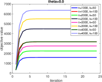
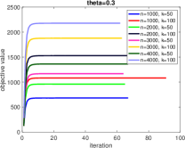
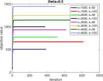
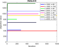
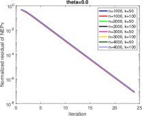
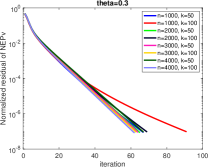
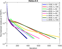
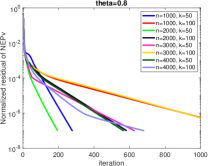
Figure 1. Convergence curves of the objective value and the normalized NEPv residual by Algorithm 1 on 8 synthetic problems for $\theta\in\{0,0.3,0.5,0.8\}$.

6.1. Experiments on Synthetic Problems

We first report numerical results on problem (1.1) solved by our proposed SCF iteration on synthetic problems, where matrices $A,B$ and $D$ are randomly generated with varying $n\in[1000,4000]$ and $k\in\{50,100\}$. Specifically, for a given pair $(n,k)$, matrix $A$ is synthesized by MATLAB as

X = randn(n, n); X = (X+X’)./2; [U,~] = eig(X);
v = rand(n,1) + 1e-6; A = U * diag(v) * U’; D = randn(n, k);

and $B$ is generated similarly to $A$. With an increase of $n$ by $1000$ in the given interval, we generated $8$ synthetic problems in total. Also varying $\theta\in[0,1]$ with an increase by $0.1$, we tested Algorithm 1 on a total of $88$ problems (1.1). The stopping tolerance ${\tt tol}=10^{-7}$ in (4.2) and the maximum number of iterations is set at $10^{3}$. We report convergence curves of both objective function value and the normalized NEPv residual as defined on the left-hand side of (4.2).

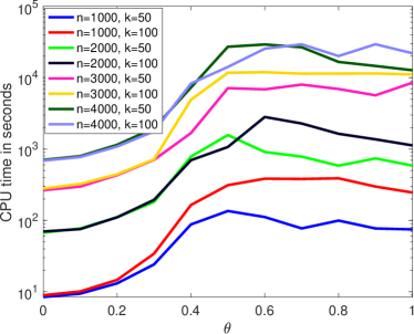
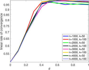
Figure 2. CPU time and the estimated linear convergence rate by Algorithm 1 on 8 synthetic problems for $\theta\in[0,1]$.

Figure 1 displays the convergence behaviors of Algorithm 1 on $8$ synthetic problems for selected $\theta\in\{0,0.3,0.5,0.8\}$. As can be observed, most of the curves of the normalized NEPv residual reach the preset tolerance ${\tt tol}=10^{-7}$ much earlier than the maximum number of iterations. For these synthetic problems, fewer numbers of iterations are required for smaller $\theta$ than larger ones. We point out that the tolerance $10^{-7}$ is often too tiny in machine learning applications. Observe that in Figure 1 all objective value curves are very much flat in fewer than 50 SCF iterations.

Figure 2 plots the CPU times by applying Algorithm 1 on $8$ synthetic problems as $\theta$ varies. These times are well correlated with the size $n$. The larger $n$ is, the more CPU time is consumed. For $\theta<0.2$, the CPU times are comparable for all problems. As $\theta$ becomes large, more CPU times are consumed for the same $(n,k)$. This observation is consistent with our estimated rates of linear convergence, which are always under $1$ (demonstrating always convergence) but increase as $\theta$ does for those synthetic problems (demonstrating more iterations are needed for a larger $\theta$ than a smaller one). We caution the reader that in general, the rate of linear convergence by Algorithm 1 is unlikely an increasing function of $\theta$ for given $A$, $B$, and $D$.

6.2. Experiments on Multi-view Data for Feature Extraction

We will specialize the blocks of $A$ and $B$ in (5.2) according to supervised multi-view subspace learning models including GMA [38], MLDA [41] and MvMDA [6] as detailed in section 5.1. The resulting concrete models under the formulation (5.4) solved by either Jacobi-style or Gauss-Seidel-style updating scheme outlined in Algorithm 1 will be named with a suffix “-J” or “-G” and a prefix “O” for “Orthogonal” (as previously in OCCA [45]). For example, OGMA-J and OGMA-G are (5.4) with $A$ and $B$ the same as the choices in GMA and solved by Algorithm 1 with Jacobi-style and Gauss-Seidel-style updating schemes, respectively.

We evaluate the model (5.4) for multi-view feature extraction in machine learning. Five datasets in Table 1 are used to evaluate the performance of the proposed six concrete models: OGMA-G, OGMA-J, OMLDA-G, OMLDA-J, OMvMDA-G, and OMvMDA-J, in terms of multi-view feature extraction by comparing them with their baseline counterparts: GMA, MLDA and MvMDA. We apply various feature descriptors to extract features of views, including CENTRIST [44], GIST [34], LBP [33], histogram of oriented gradient (HOG), color histogram (CH), and SIFT-SPM [21], from image datasets: Caltech101 [22] and Scene15 [21]. Multiple Features (mfeat) and Internet Advertisements (Ads) are publicly available from the UCI machine learning repository [11]. Dataset mfeat contains handwritten numeral data with six views including profile correlations (fac), Fourier coefficients of the character shapes (fou), Karhunen-Love coefficients (kar), morphological features (mor), pixel averages in $2\times 3$ windows (pix), and Zernike moments (zer). Ads is used to predict whether or not a given hyperlink (associated with an image) is an advertisement and has three views: features based on the terms in the images URL, caption, and alt text (url+alt+caption), features based on the terms in the URL of the current site (origurl), and features based on the terms in the anchor URL (ancurl).

Except for MvMDA and its new variants: OMvMDA-G and OMvMDA-J, all other methods share the same trade-off parameter $\alpha$ to balance the pairwise correlations and supervised information. In our experiments, we tune $\alpha\in\{0.01,0.1,1,10,100\}$ for proper balancing in supervised setting. To prevent possible singularity in matrix $B$, we add a small value, e.g., $10^{-8}$, to the diagonals of $B_{s}\,\forall s$. For our proposed methods, an additional parameter $\theta$ is varied from $0$ to $1$ with an increase of $0.1$. We also set the maximum number of iterations to $50$ for both the SCF iteration of Algorithm 1 and the Jacobi-style or Gauss-Seidel-style updating of Algorithm 1. It is more of an empirical threshhold observed as a good enough setting for multi-view feature extraction.

Table 1. Real world data sets, where the number of features for each view is shown inside the bracket and ‘-’ for views not applicable.

	mfeat	Caltech101-7	Caltech101-20	Scene15	Ads
samples	2000	1474	2386	4310	3279
classes	10	7	20	15	2
view 1	fac(216)	CENTRIST(254)	CENTRIST(254)	CENTRIST(254)	url+alt+caption(588)
view 2	fou(76)	GIST(512)	GIST(512)	GIST(512)	origurl(495)
view 3	kar(64)	LBP(1180)	LBP(1180)	LBP(531)	ancurl(472)
view 4	mor(6)	HOG(1008)	HOG(1008)	HOG(360)	-
view 5	pix(240)	CH(64)	CH(64)	SIFT-SPM(1000)	-
view 6	zer(47)	SIFT-SPM(1000)	SIFT-SPM(1000)	-	-

To evaluate the classification performance of compared methods, the 1-nearest neighbor classifier as the base classifier is employed. We run each method to learn projection matrices by varying the dimension of the common subspace $k\in\{2,3,5:5:30\}$ for all datasets except $k\in\{2,3,4,5,6\}$ for mfeat due to its smallest view mor having only $6$ features. We split each dataset into training and testing with ratio 10/90. The learned projection matrices are used to transform both training and testing data into the latent common space, and then the classifier is trained and tested in this space. Following [45], the serial feature fusion strategy is employed by concatenating projected features from all views. Classification accuracy is used to measure learning performance. Experimental results are reported in terms of the average and standard deviation over 10 randomly drawn splits.

Table 2. Classification accuracy ($\pm$ standard deviation) of multi-view feature extraction on five real world data sets with 10% training and 90% testing over 10 random splits. The best $\theta$ is shown in the bracket.

methods	mfeat	Caltech101-7	Caltech101-20	Scene15	Ads
GMA	93.99 $\pm$ 0.87	93.25 $\pm$ 1.04	81.16 $\pm$ 0.94	61.41 $\pm$ 1.30	92.59 $\pm$ 1.76
OGMA-J	96.81 $\pm$ 0.46(0.4)	95.14 $\pm$ 0.59(0.4)	86.48 $\pm$ 1.02(0.6)	79.90 $\pm$ 0.80(1.0)	94.69 $\pm$ 0.75(0.8)
OGMA-G	96.80 $\pm$ 0.44(0.4)	95.07 $\pm$ 0.56(0.5)	86.60 $\pm$ 1.11(0.5)	79.90 $\pm$ 1.02(1.0)	94.91 $\pm$ 0.67(0.8)
MLDA	92.01 $\pm$ 1.74	92.18 $\pm$ 0.95	77.79 $\pm$ 1.01	59.02 $\pm$ 0.94	92.50 $\pm$ 2.06
OMLDA-J	96.74 $\pm$ 0.40(0.8)	94.68 $\pm$ 0.48(0.8)	86.23 $\pm$ 1.16(0.9)	81.42 $\pm$ 1.07(1.0)	94.79 $\pm$ 0.65(0.8)
OMLDA-G	96.82 $\pm$ 0.38(0.8)	94.59 $\pm$ 0.62(0.3)	86.09 $\pm$ 1.22(0.9)	80.68 $\pm$ 0.88(1.0)	94.76 $\pm$ 0.74(0.8)
MvMDA	93.78 $\pm$ 0.91	92.14 $\pm$ 0.68	79.27 $\pm$ 1.71	57.33 $\pm$ 1.18	78.51 $\pm$ 2.96
OMvMDA-J	96.62 $\pm$ 0.31(0.5)	95.11 $\pm$ 0.72(0.4)	85.69 $\pm$ 0.87(0.4)	77.98 $\pm$ 1.24(0.9)	94.02 $\pm$ 1.54(0.6)
OMvMDA-G	96.63 $\pm$ 0.37(0.4)	94.95 $\pm$ 0.56(0.5)	85.76 $\pm$ 1.00(0.4)	78.07 $\pm$ 0.83(0.9)	93.52 $\pm$ 0.59(0.0)

Table 2 shows the classification accuracies and standard deviations of $9$ multi-view feature extraction methods on five real data sets over 10 random splits with 10% training and 90% testing. We have observed the following:

1. Our proposed methods consistently outperform their counterparts on all five data sets. The least improvement by about 2% on Ads is observed, while the largest improvement occurs on Scene15 for about 20%.

2. The Jacobi-style and Gauss-Seidel-style updating schemes on the same model achieve similar classification accuracies with differences falling within 0.8%.

3. MvMDA on Ads fails to produce a proper latent representation since its accuracy is 14% less than those of GMA and MLDA. However, OMvMDA-J and OMvMDA-G perform very well on the same data set.

4. Accuracies by all 6 proposed models are comparable and very good. This may be due to our trace ratio formulation with its orthogonal projection matrices for noisy robustness [45] as well as the varying $\theta$ for weighting.

	Caltech101-7	Scene15	Ads
varying $\theta$
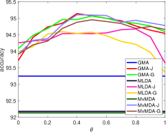
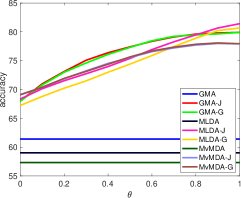
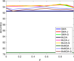
varying $k$

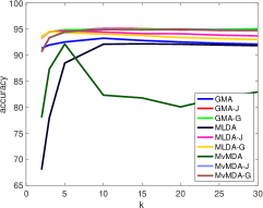
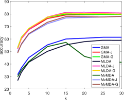
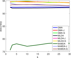
Figure 3. Accuracies of compared methods on three data sets by varying $k\in[2,6]$ and $\theta\in[0,1]$.

In Figure 3 (the 1st row), we also report the classification accuracy of $9$ methods with varying $\theta\in[0,1]$. On Caltech101-7, Caltech101-20 and mfeat, the best results of our proposed methods are roughly around $\theta=0.5$. However, different behaviors are found on Scene15 and Ads. $\theta$ does not show significantly impact on Ads, but it produces better accuracy on Scene15 as $\theta$ increases. For almost all $\theta$, our proposed methods consistently outperform baselines. This implies that $\theta$ introduced in (5.4) can be useful to find better projection matrices for multi-view feature extraction. We further show the trend of classification accuracy of compared methods by varying the dimension of latent common space $k$ in Figure 3 (the 2nd row). For any fixed $k$, our proposed methods outperform their counterparts. Importantly, our proposed methods nearly reach their best performances all for fairly small $k$, while baseline methods have to use larger $k$ to match that. This can be plausibly explained, namely, orthonormal bases retain less redundant information than non-orthonormal ones. We also observed that MvMDA behaves unstably for large $k$ on Caltech101-7 and Scene15 since the accuracy drops too significantly but this does not happen to OMvMDA-G and OMvMDA-J. In summary, our proposed models not only demonstrate superior performances to baseline methods but also are more robust to data noise and can achieve the same or better performance at smaller $k$. Small $k$ implies fast computations if an iterative eigen-solver [2, 15, 25] is used in Algorithm 1 and that is extremely useful for large scale real world applications, such as cross-modal retrieval [6], for a fast response time due to less computation costs of pairwise distances in a lower dimensional space.

7. Conclusions

We have completed a thorough investigation, both in theory and numerical solutions, of the trace ratio maximization problem

$$\max_{X^{\operatorname{T}}X=I_{k}}\frac{\operatorname{trace}(X^{\operatorname{T}}AX+X^{\operatorname{T}}D)}{[\operatorname{trace}(X^{\operatorname{T}}BX)]^{\theta}}.$$

At least three special cases of it have been well studied in the past decades because of their immediate applications to data science. Our main results include an NEPv (nonlinear eigenvalue problem with eigenvector dependency, a term coined in [5]) formulation of its KKT condition, necessary conditions for its local and global maximizers, a complete picture of the role played by $D$ on the maximizers, a guaranteed convergent numerical method and its full convergent analysis. As an application of these results, we propose a new orthogonal multi-view subspace framework and experiment on its 6 instantiated models in either supervised or unsupervised setting. Numerical results demonstrate the new models often outperform existing baselines.

Although we have been limiting our discussion on real matrices, the developments in this paper can be straightforwardly extended to complex matrices with minor modifications, namely, replace all $\mathbb{R}$ by $\mathbb{C}$ (complex numbers) and all transposes $\operatorname{T}$ by complex conjugate transpose $\operatorname{H}$.

References

- [1] Absil, P.A., Mahony, R., Sepulchre, R.: Optimization Algorithms On Matrix Manifolds. Princeton University Press (2008)
- [2] Bai, Z., Demmel, J., Dongarra, J., Ruhe, A., van der Vorst (editors), H.: Templates for the solution of Algebraic Eigenvalue Problems: A Practical Guide. SIAM, Philadelphia (2000)
- [3] Baltrušaitis, T., Ahuja, C., Morency, L.P.: Multimodal machine learning: A survey and taxonomy. IEEE Trans. Pattern Anal. Mach. Intell. 41(2), 423–443 (2018)
- [4] Borg, I., Lingoes, J.: Multidimensional Similarity Structure Analysis. Springer-Verlag, New York (1987)
- [5] Cai, Y., Zhang, L.H., Bai, Z., Li, R.C.: On an eigenvector-dependent nonlinear eigenvalue problem. SIAM J. Matrix Anal. Appl. 39(3), 1360–1382 (2018)
- [6] Cao, G., Iosifidis, A., Chen, K., Gabbouj, M.: Generalized multi-view embedding for visual recognition and cross-modal retrieval. IEEE Trans. Cybernetics 48(9), 2542–2555 (2018)
- [7] Chu, M.T., Trendafilov, N.T.: The orthogonally constrained regression revisited. J. Comput. Graph. Stat. 10(4), 746–771 (2001)
- [8] Cunningham, J.P., Ghahramani, Z.: Linear dimensionality reduction: Survey, insights, and generalizations. J. Mach. Learning Res. 16, 2859–2900 (2015)
- [9] Demmel, J.: Applied Numerical Linear Algebra. SIAM, Philadelphia, PA (1997)
- [10] Dinkelbach, W.: On nonlinear fractional programming. Management Science 13(7), 492–498 (1967)
- [11] Dua, D., Graff, C.: UCI machine learning repository (2017). http://archive.ics.uci.edu/ml
- [12] Edelman, A., Arias, T.A., Smith, S.T.: The geometry of algorithms with orthogonality constraints. SIAM J. Matrix Anal. Appl. 20(2), 303–353 (1999)
- [13] Eldén, L., Park, H.: A procrustes problem on the Stiefel manifold. Numer. Math. 82, 599–619 (1999)
- [14] de Geer, J.P.V.: Linear relations among sets of variables. Psychometrika 49, 70–94 (1984)
- [15] Golub, G.H., Van Loan, C.F.: Matrix Computations, 4th edn. Johns Hopkins University Press, Baltimore, Maryland (2013)
- [16] Gower, J.C., Dijksterhuis, G.B.: Procrustes Problems. Oxford University Press, New York (2004)
- [17] Horn, R.A., Johnson, C.R.: Topics in Matrix Analysis. Cambridge University Press, Cambridge (1991)
- [18] Hurley, J.R., Cattell, R.B.: The Procrustes program: producing direct rotation to test a hypothesized factor structure. Beh. Sci. 7, 258–262 (1962)
- [19] Kanzow, C., Qi, H.D.: A QP-free constrained Newton-type method for variational inequality problems. Math. Program. 85, 81–106 (1999)
- [20] Kushmerick, N.: Learning to remove internet advertisements. In: Proceedings of the third annual conference on Autonomous Agents, pp. 175–181 (1999)
- [21] Lazebnik, S., Schmid, C., Ponce, J.: Beyond bags of features: Spatial pyramid matching for recognizing natural scene categories. In: 2006 IEEE Computer Society Conference on Computer Vision and Pattern Recognition (CVPR’06), vol. 2, pp. 2169–2178. IEEE (2006)
- [22] Li, F.F., Fergus, R., Perona, P.: Learning generative visual models from few training examples: An incremental bayesian approach tested on 101 object categories. Computer Vision and Image Understanding 106(1), 59–70 (2007)
- [23] Li, R.C.: A perturbation bound for the generalized polar decomposition. BIT 33, 304–308 (1993)
- [24] Li, R.C.: New perturbation bounds for the unitary polar factor. SIAM J. Matrix Anal. Appl. 16, 327–332 (1995)
- [25] Li, R.C.: Rayleigh quotient based optimization methods for eigenvalue problems. In: Z. Bai, W. Gao, Y. Su (eds.) Matrix Functions and Matrix Equations, Series in Contemporary Applied Mathematics, vol. 19, pp. 76–108. World Scientific, Singapore (2015). Lecture summary for 2013 Gene Golub SIAM Summer School
- [26] Li, W., Sun, W.: Perturbation bounds for unitary and subunitary polar factors. SIAM J. Matrix Anal. Appl. 23, 1183–1193 (2002)
- [27] Liu, X.G., Wang, X.F., Wang, W.G.: Maximization of matrix trace function of product Stiefel manifolds. SIAM J. Matrix Anal. Appl. 36(4), 1489–1506 (2015)
- [28] Martin, R.M.: Electronic Structure: Basic Theory and Practical Methods. Cambridge University Press, Cambridge, UK (2004)
- [29] Moré, J.J., Sorensen, D.C.: Computing a trust region step. SIAM J. Sci. Statist. Comput. 4(3), 553–572 (1983)
- [30] von Neumann, J.: Some matrix-inequalities and metrization of matrix-space. Tomck. Univ. Rev. 1, 286–300 (1937)
- [31] Ngo, T., Bellalij, M., Saad, Y.: The trace ratio optimization problem for dimensionality reduction. SIAM J. Matrix Anal. Appl. 31(5), 2950–2971 (2010)
- [32] Nie, F., Zhang, R., X.Li: A generalized power iteration method for solving quadratic problem on the Stiefel manifold. SCIENCE CHINA Info. Sci. 60, 112101:1–112101:10 (2017)
- [33] Ojala, T., Pietikäinen, M., Mäenpää, T.: Multiresolution gray-scale and rotation invariant texture classification with local binary patterns. IEEE Trans. Pattern Anal. Mach. Intell. 24(7), 971–987 (2002)
- [34] Oliva, A., Torralba, A.: Modeling the shape of the scene: A holistic representation of the spatial envelope. International Journal of Computer Vision 42(3), 145–175 (2001)
- [35] Peng, Y., Qi, J.: CM-GANs: Cross-modal generative adversarial networks for common representation learning. ACM Transactions on Multimedia Computing, Communications, and Applications (TOMM) 15(1), 1–24 (2019)
- [36] Saad, Y., Chelikowsky, J.R., Shontz, S.M.: Numerical methods for electronic structure calculations of materials. SIAM Rev. 52(1), 3–54 (2010)
- [37] Seber, G.A.F.: A Matrix Handbook for Statisticians. Wiley, New Jersey (2007)
- [38] Sharma, A., Kumar, A., Daume, H., Jacobs, D.W.: Generalized multiview analysis: A discriminative latent space. In: 2012 IEEE Conference on Computer Vision and Pattern Recognition, pp. 2160–2167. IEEE (2012)
- [39] Stewart, G.W.: Matrix Algorithms, Vol. II: Eigensystems. SIAM, Philadelphia (2001)
- [40] Sun, J.G.: Matrix Perturbation Analysis. Academic Press, Beijing (1987). In Chinese.
- [41] Sun, S., Xie, X., Yang, M.: Multiview uncorrelated discriminant analysis. IEEE Trans. Cybernetics 46(12), 3272–3284 (2016)
- [42] Vía, J., Santamaría, I., Pérez, J.: A learning algorithm for adaptive canonical correlation analysis of several data sets. Neural Networks 20(1), 139–152 (2007)
- [43] Wang, H., Yan, S., Xu, D., Tang, X., Huang, T.: Trace ratio vs. ratio trace for dimensionality reduction. In: 2007 IEEE Conference on Computer Vision and Pattern Recognition, pp. 1–8. IEEE (2007)
- [44] Wu, J., Rehg, J.M.: Where am i: Place instance and category recognition using spatial pact. In: 2008 IEEE Conference on Computer Vision and Pattern Recognition, pp. 1–8. IEEE (2008)
- [45] Zhang, L., Wang, L., Bai, Z., Li, R.C.: A self-consistent-field iteration for orthogonal canonical correlation analysis. IEEE Trans. Pattern Anal. Mach. Intell. (2020). doi10.1109/TPAMI.2020.3012541
- [46] Zhang, L.H., Liao, L.Z., Ng, M.K.: Fast algorithms for the generalized Foley-Sammon discriminant analysis. SIAM J. Matrix Anal. Appl. 31(4), 1584–1605 (2010)
- [47] Zhang, L.H., Liao, L.Z., Ng, M.K.: Superlinear convergence of a general algorithm for the generalized Foley-Sammon discriminant analysis. J. Optim. Theory Appl. 157(3), 853–865 (2013)
- [48] Zhang, L.H., Yang, W.H., Shen, C., Ying, J.: An eigenvalue-based method for the unbalanced Procrustes problem. SIAM J. Matrix Anal. Appl. 41(3), 957–983 (2020)
- [49] Zhang, Z.Y., Du, K.Q.: Successive projection method for solving the unbalanced procrustes problem. SCIENCE CHINA Math. 49(7), 971–986 (2006)
- [50] Zhao, H., Wang, Z., Nie, F.: Orthogonal least squares regression for feature extraction. Neurocomputing 216, 200–207 (2016)