Solving Common-Payoff Games with Approximate Policy Iteration

Abstract

For artificially intelligent learning systems to have widespread applicability in real-world settings, it is important that they be able to operate decentrally. Unfortunately, decentralized control is difficult—computing even an epsilon-optimal joint policy is a NEXP complete problem. Nevertheless, a recently rediscovered insight—that a team of agents can coordinate via common knowledge—has given rise to algorithms capable of finding optimal joint policies in small common-payoff games. The Bayesian action decoder (BAD) leverages this insight and deep reinforcement learning to scale to games as large as two-player Hanabi. However, the approximations it uses to do so prevent it from discovering optimal joint policies even in games small enough to brute force optimal solutions. This work proposes CAPI, a novel algorithm which, like BAD, combines common knowledge with deep reinforcement learning. However, unlike BAD, CAPI prioritizes the propensity to discover optimal joint policies over scalability. While this choice precludes CAPI from scaling to games as large as Hanabi, empirical results demonstrate that, on the games to which CAPI does scale, it is capable of discovering optimal joint policies even when other modern multi-agent reinforcement learning algorithms are unable to do so.

Introduction

In reinforcement learning (Sutton and Barto 2018), an agent seeks to learn a policy that extracts a large return from an environment, making it an algorithmic formulation of choice for many control problems. However, the standard reinforcement learning framework assumes that decision making is centralized. In general, a control problem may require multiple decision makers to act in a setting that bars complete information sharing, often in practice because decision makers are spatially separated. This problem is known as decentralized control and has been studied by a number of different communities using varying formalisms (Yu-Chi Ho 1980; Oliehoek and Amato 2016; Littman 1994), which we collectively refer to as common-payoff games (Leyton-Brown and Shoham 2008).

Despite involving multiple agents, the decentralized control problem bears relatively little similarity to general game-theoretic settings (Powers and Shoham 2004), in which agents possess adversarial incentives and there is not a generally agreed upon notion of optimality. It is also distinct from other problem settings operating under common-payoff game formalisms, such as ad-hoc coordination (Stone et al. 2010), in which some of the agents are externally specified, or emergent communication (Lazaridou, Peysakhovich, and Baroni 2017), in which coordination must arise naturally (not from precoordinated learning procedures). Instead, in the decentralized control problem, the entity seeking to maximize return specifies all agents, including possibly precoordinated learning procedures.

While the decentralized control problem bears resemblance to the classical reinforcement problem in that both involve maximizing expected return, decentralized control presents challenges that do not arise in classical reinforcement learning. Most notably, dynamic programming is not directly applicable to agents in decentralized control problems because the value of an agent’s information state depends on the policies of its teammates. One way to circumvent this issue is by alternating maximization (Nair et al. 2003). Each agent maximizes its policy in turn, holding the policies of its teammates fixed. This procedure guarantees convergence to a Nash equilibrium, but can be arbitrarily far away from an optimal joint policy, as measured by expected return. Independent reinforcement learning (IRL) (Tan 1997), a paradigm in which all agents concurrently execute reinforcement learning algorithms, is another approach to dealing with decentralized control problems that has been the subject of attention in the deep multi-agent reinforcement learning community. However, the convergence guarantees of IRL are less well-understood than those of alternating maximization and those that do exist show convergence only to local optima (Bono et al. 2018; Claus and Boutilier 1998).

Arguably the most exciting line of research over the last decade in the pursuit of optimal joint policies for common-payoff games stems from the seminal insight of Nayyar, Mahajan, and Teneketzis (Nayyar, Mahajan, and Teneketzis 2013). In their work, they show that, by conditioning on common knowledge, a team of decentralized agents can effectively act as a single agent, allowing for the direct application dynamic programming and resolving the difficulty of joint exploration. But conditioning on common knowledge is not a panacea. Finding an optimal, or even $\epsilon$-optimal, joint policy for a Dec-POMDP (Oliehoek and Amato 2016), the standard formalism for common-payoff games, is a NEXP-complete problem (Bernstein et al. 2000; Rabinovich, Goldman, and Rosenschein 2003). While Nayyar, Mahajan, and Teneketzis’s insights lead to solution methods for toy games, they are not immediately applicable to larger games, as conditioning on common knowledge is an exponential reduction. And while there has significant progress in scaling similar ideas in the Dec-POMDP community (Dibangoye et al. 2016; Dibangoye and Buffet 2018), resulting algorithms have largely been restricted to games having hundreds of states and fewer than ten actions.

At the time of writing, the Bayesian action decoder (BAD) (Foerster et al. 2019) is the only attempt that has been made to scale Nayyar, Mahajan, and Teneketzis’s common knowledge approach to very large settings. BAD is a policy-based approach relying on deep learning and independence assumptions. When combined with population based training, BAD achieves good performance in two-player Hanabi. However, while BAD achieves its intent of scalability, the approximations it requires to do so are so compromising that it struggles to solve games small enough to brute force an optimal solution.

Ideally there would an exist a common-knowledge approach matching or exceeding BAD’s performance on large games that was also capable of solving small and medium-sized games. This work takes a first step toward this goal by introducing cooperative approximate policy iteration (CAPI), a novel deep approximate policy iteration algorithm for common-payoff imperfect information games. Like BAD, CAPI seeks to scale Nayyar, Mahajan, and Teneketzis’s insights. But unlike BAD, CAPI prioritizes recovering the optimal joint policy over scalability. To demonstrate the efficacy of CAPI, we consider two common-payoff games from OpenSpiel. Having as many as tens of thousands of states and as many as hundreds of actions, these games are two orders of magnitudes larger than the common-payoff games that are often considered in Dec-POMDP literature (Dibangoye et al. 2016). We show that CAPI is able to achieve strong performance, solving (discovering an optimal policy of) both games a majority of the time.

Background

Public and Common Knowledge

Common knowledge has long been a subject of investigation in philosophy (Vanderschraaf and Sillari 2013; Lewis 1969), multi-agent systems (Halpern and Moses 2000), and (epistemic) game theory (Aumann 1976; Pacuit and Roy 2015; Perea 2012). Let $K_{1}^{G}$ be the set of information known to all agents in group $G$. Let $K_{i+1}^{G}$ be the subset of $K_{i}^{G}$ that is known by all agents to be in $K_{i}^{G}$. Then

$$K_{\mbox{common}}^{G}\coloneqq\cap_{i=1}^{\infty}K_{i}^{G}$$

is common knowledge among $G$. The significance of common knowledge is that the inclusion status of any proposition is known by every member of the group. In general, the same cannot be said for the set $K_{i}^{G}$ for any $i\in\mathbb{N}$. This distinction has important implications regarding the abilities of groups of agents to coordinate their actions.

Unfortunately, while common knowledge appears to be essential for coordination in many settings, the infinite regress that defines it can make it expensive to compute (Schroeder de Witt, Foerster et al. 2019; Kovarík et al. 2019; Šustr, Kovařík, and Lisý 2019; Clark and Marshall 1981; Halpern and Moses 2000). In imperfect information games, a recent effort to circumvent this issue focuses attention on public knowledge, a special subset of common knowledge that is easily computable (Kovarík et al. 2019). Specifically, public knowledge is the subset $K_{\mbox{public}}^{G}\subset K_{\mbox{common}}^{G}$ of common knowledge that is publicly announced as such.

Factored Observation Stochastic Games

This work adopts finite common-payoff factored-observation stochastic game (FOSG) formalism (Kovarík et al. 2019). Finite common-payoff FOSGs have sufficient expressive power to represent finite Dec-POMDPs, the standard formalism for common-payoff games, and handle public knowledge in a principled manner. A common-payoff FOSG is a tuple $G=\langle\mathcal{N},\mathcal{W},w^{0},\mathcal{A},\mathcal{T},\mathcal{R},\mathcal{O}\rangle$ where

• $\mathcal{N}=\{1,\dots,N\}$ is the player set.

• $\mathcal{W}$ is the set of world states and $w^{0}$ is a designated initial state.

• $\mathcal{A}=\mathcal{A}_{1}\times\cdots\times\mathcal{A}_{N}$ is the space of joint actions.

• $\mathcal{T}$ is the transition function mapping $\mathcal{W}\times\mathcal{A}\to\Delta(\mathcal{W})$.

• $\mathcal{R}{=}(\mathcal{R}_{1},\dots,\mathcal{R}_{N})$ and $\mathcal{R}_{1}{=}\cdots{=}\mathcal{R}_{N}\colon\mathcal{W}\times\mathcal{A}\to\mathbb{R}$ is the reward function.

• $\mathcal{O}=(\mathcal{O}_{\mbox{priv}(1)},\dots,\mathcal{O}_{\mbox{priv}(N)},\mathcal{O}_{\mbox{pub}})$ is the observation function where

  • $\mathcal{O}_{\mbox{priv}(i)}\colon\mathcal{W}\times\mathcal{A}\times\mathcal{W}\to\mathbb{O}_{\mbox{priv}(i)}$ specifies the private observation that player $i$ receives.

  • $\mathcal{O}_{\mbox{pub}}\colon\mathcal{W}\times\mathcal{A}\times\mathcal{W}\to\mathbb{O}_{\mbox{pub}}$ specifies the public observation that all players receive.

  • $O_{i}{=}\mathcal{O}_{i}(w,a,w^{\prime}){=}(\mathcal{O}_{\mbox{priv}(i)}(w,a,w^{\prime}),\mathcal{O}_{\mbox{pub}}(w,a,w^{\prime}))$ is player $i$’s observation.

Note that actions need not be observable in FOSGs.

There are also a number of important derived objects in FOSGs.

• A history is a finite sequence $h=(w^{0},a^{0},\dots,w^{t})$. We write $g\sqsubseteq h$ when $g$ is a prefix of $h$.

• The set of histories is denoted by $\mathcal{H}$.

• The information state for player $i$ at $h=(w^{0},a^{0},\dots,w^{t})$ is $s_{i}(h)\coloneqq(O_{i}^{0},a_{i}^{0},\dots,O_{i}^{t})$.

• The information state space for player $i$ is
  $\mathcal{S}_{i}\coloneqq\{s_{i}(h)\mid h\in\mathcal{H}\}$.

• The legal actions for player $i$ at $s_{i}$ is denoted $\mathcal{A}_{i}(s_{i})$.

• A joint policy is a tuple $\pi=(\pi_{1},\dots,\pi_{N})$, where policy $\pi_{i}$ maps $\mathcal{S}_{i}\to\Delta(\mathcal{A}_{i})$.

• The public state at $h$ is the sequence
  $s_{\mbox{pub}}(h)\coloneqq s_{\mbox{pub}}(s_{i}(h))\coloneqq(O_{\mbox{pub}}^{0},\dots,O_{\mbox{pub}}^{t})$.

• The public tree $\mathcal{S}_{\mbox{pub}}$ is the space of public states.

• The public set for $s\in\mathcal{S}_{\mbox{pub}}$ is $I_{\mbox{pub}}(s){\coloneqq}\{h\mid s_{\mbox{pub}}(h)=s\}$.

• The information state set for player $i$ at $s\in\mathcal{S}_{\mbox{pub}}$ is $\mathcal{S}_{i}(s)\coloneqq\{s_{i}\in\mathcal{S}_{i}\mid s_{\mbox{pub}}(s_{i})=s\}$.

• The reach probability of $h$ under $\pi$ is
  $P^{\pi}(h)=P_{\mathcal{T}}(h)\prod_{i\in\mathcal{N}}P_{i}^{\pi}(h)$ where

  • Chance’s contribution is
    $P_{\mathcal{T}}(h)\coloneqq\prod_{h^{\prime}aw\sqsubseteq h}\mathcal{T}(h^{\prime},a,w)$.

  • Player $i$’s contribution is
    $P^{\pi}_{i}(h)\coloneqq P^{\pi}_{i}(s_{i}(h))\coloneqq\prod_{s_{i}^{\prime}a\sqsubseteq s_{i}(h)}\pi_{i}(s_{i}^{\prime},a)$.

Public Knowledge in Common-Payoff Games

Nayyar, Mahajan, and Teneketzis (Nayyar, Mahajan, and Teneketzis 2013) were the first to formalize the general importance of public knowledge for coordinating teams of agents in common-payoff games. They introduce the partial history sharing information structure, a model for decentralized stochastic control resembling common-payoff FOSGs in that it explicitly acknowledges public observations. Nayyar, Mahajan, and Teneketzis show that this structure can be converted into a POMDP, which we refer to as the public POMDP. Given a common-payoff FOSG $\langle\mathcal{N},\mathcal{W},w^{0},\mathcal{A},\mathcal{T},\mathcal{R},\mathcal{O}\rangle$, we can construct a public POMDP $\langle\tilde{\mathcal{W}},\tilde{w}^{0},\tilde{\mathcal{A}},\tilde{\mathcal{T}},\tilde{\mathcal{R}},\tilde{\mathcal{O}}\rangle$ as follows.

• The world states of the public POMDP $\tilde{\mathcal{W}}$ are the histories $\mathcal{H}$ of the common-payoff FOSG.

• The initial world state of the public POMDP $\tilde{w}^{0}$ is the one tuple $(w^{0})$.

• The actions of the public POMDP are called prescription vectors. A prescription vector is denoted by $\Gamma$ and has $N$ components. The $i$th component of a prescription vector $\Gamma_{i}$ is the prescription for player $i$. A prescription $\Gamma_{i}$ maps $s_{i}$ to an element of $\mathcal{A}_{i}(s_{i})$ for each $s_{i}\in\mathcal{S}_{i}(s_{\mbox{pub}}(h))$. In words, a prescription instructs a player in the common-payoff FOSG how to act as a function of its private information. An example is shown in Figure 1.

• Given $\tilde{w}\equiv h$ and $\Gamma$, the transition distribution $\tilde{\mathcal{T}}(\tilde{w},\Gamma)$ is induced by $\mathcal{T}(h,a)$, where

  $$a\equiv\Gamma(h)\coloneqq\left(\Gamma_{1}(s_{1}(h)),\dots,\Gamma_{N}(s_{N}(h))\right).$$

• Given $\tilde{w}\equiv h$ and $\tilde{w}^{\prime}\equiv h^{\prime}$, the reward $\tilde{\mathcal{R}}(\tilde{w},\Gamma,\tilde{w}^{\prime})\equiv\mathcal{R}_{1}(h,\Gamma(h),h^{\prime})=\cdots=\mathcal{R}_{N}(h,\Gamma(h),h^{\prime})$.

• Given $\tilde{w}\equiv h$ and $\tilde{w}^{\prime}\equiv h^{\prime}$, the observation $\tilde{\mathcal{O}}(\tilde{w},\Gamma,\tilde{w}^{\prime})\equiv\mathcal{O}_{\mbox{pub}}(h,\Gamma(h),h^{\prime})$.

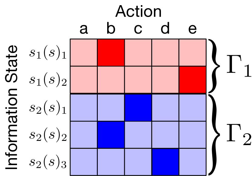
Figure 1: An example prescription vector. There are two players, with five actions each. Player one (red) has two possible information states while player two (blue) has three. The prescription vector decides each player’s action as a function of its information state, as shown by the darkened squares.

In summary, the public POMDP can be informally described as involving a coordinator who only observes public observations and instructs the players how to act based on these observations. One can imagine that this formulation could be executed at test time in a decentralized fashion by having each player carry around an identical copy of the central coordinator. Since each player feeds its copy of the coordinator the same public observations, each copy of the coordinator produces the same prescription vector and it is as if a single coordinator were acting in the public POMDP.

As with any with POMDP, the public POMDP can also be considered as a belief MDP, as is exampled in Figure 2. We follow the precedent set by Foerster et al., who refer to this perspective as the public belief MDP (PuB-MDP).

The public POMDP and PuB-MDP have proven highly valuable and have been applied extensively in control literature (Gagrani and Nayyar 2018; Afshari and Mahajan 2018; Vasconcelos and Martins 2016; Arabneydi and Mahajan 2014; Gagrani and Nayyar 2017; Ouyang, Asghari, and Nayyar 2018; Lessard and Nayyar 2013; Tavafoghi, Ouyang, and Teneketzis 2018, 2016; Ouyang, Tavafoghi, and Teneketzis 2015; Zhang, Miehling, and Başar 2019; Nayyar et al. 2014; Gupta 2020) and, to a lesser extent, reinforcement learning (Foerster et al. 2019; Hadfield-Menell et al. 2016; Arabneydi and Mahajan 2015) literature. Unfortunately, the public POMDP is so massive (there are roughly $|\mathcal{A}_{i}|^{N\cdot|\mathcal{S}_{i}|}$ actions at each decision point) that it is infeasible to apply POMDP solution methods (Hausknecht and Stone 2015; Silver and Veness 2010; Somani et al. 2013; Smith and Simmons 2012; Pineau, Gordon, and Thrun 2006; Ross et al. 2008; Spaan and Vlassis 2005; Shani, Pineau, and Kaplow 2013), out-of-the-box, to common-payoff games of non-trivial size.

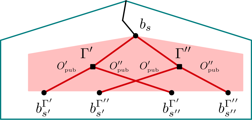
Figure 2: A visualization of a decision point in the PuB-MDP. The game begins in state $b_{s}$, a distribution over the public set $I_{\mbox{pub}}(s)$. The coordinator is given a choice between two possible prescriptions $\Gamma^{\prime}$ and $\Gamma^{\prime\prime}$. Both choices generate observations $O_{\mbox{pub}}^{\prime}$ and $O_{\mbox{pub}}^{\prime\prime}$ with positive probabilities (inducing public states $s^{\prime}$ and $s^{\prime\prime}$ respectively). Accordingly, there are four possible belief states for the next time step.

The Tiny Hanabi Suite

To emphasize the contrast in guarantees between algorithms running in the PuB-MDP and independent learning algorithms, we display results from the Tiny Hanabi Suite—a collection of six very small Dec-POMDPs detailed in the appendix. We compare independent Q-learning (IQL), hysteretic Q-learning (HQL) (Matignon, Laurent, and Le Fort-Piat 2007), independent advantage actor centralized critic (IA2C2) (Lowe et al. 2017; Foerster et al. 2017), value decomposition networks (VDN) (Sunehag, Lever et al. 2017), simplified action decoding (SAD) (Hu and Foerster 2020), and Q-learning in the PuB-MDP. All algorithms were implemented tabularly and tuned across nine hyperparameter settings. The results shown in Figure 3 are averages over 32 runs. Code for the Tiny Hanabi Suite is available at https://github.com/ssokota/tiny-hanabi.

Despite tuning, reinforcement learning algorithms perform poorly. HQL, VDN and SAD solve only four of the six games, IQL solves only three, and IA2C2 solves only one. In contrast, Q-learning in the PuB-MDP solves all six games. There results reaffirm that the differences in guarantees between algorithms that operate in the PuB-MDP and algorithms that operate within the independent reinforcement learning paradigm are not just theoretical—they also manifest in practice, even for modern multi-agent reinforcement learning algorithms.

Cooperative Approximate Policy Iteration

In this section, we introduce CAPI, a novel instance of approximate policy iteration operating within the PuB-MDP. At a high level, at each decision point, CAPI generates a large number of prescription vectors using a policy and evaluates each of these prescription vectors according to its expected reward and the expected estimated value of the next belief state, selecting the most highly assessed prescription vector as its action. We provide pseudocode for CAPI in Algorithm 1. Each step is explained in greater detail below.

1. At each decision point, CAPI takes a belief state $b$ and a number of rollouts $K$ as argument.

2. CAPI produces its policy $\pi(b)$ (over prescription vectors) as a function of the belief state. CAPI can either keep a separate tabular policy for each public state in the game or produce it by passing the belief state through a neural network.

3. CAPI acquires $K$ prescription vectors as a function of the policy $\pi(b)$. Acquisition can be done either by sampling or taking the $K$-most-likely.

4. CAPI evaluates each of the $K$ prescription vectors. For each prescription vector $\Gamma^{(k)}$, this involves

   1. Computing expected reward $r^{(k)}$ for $\Gamma^{(k)}$ given $b$.

   2. Computing the next belief state $b^{(k,O_{\mbox{pub}})}$ for each $O_{\mbox{pub}}$.

   3. Estimating the value $v^{(k,O_{\mbox{pub}})}$ of $b^{(k,O_{\mbox{pub}})}$ using the value network.

   4. Computing the probability distribution $p^{(k)}$ over public observations given $b$ and $\Gamma^{(k)}$.

   The assessed value is the expected reward plus the expected estimated value of the next belief state

   $$q^{(k)}\leftarrow r^{(k)}+\underset{O_{\mbox{pub}}\sim p^{(k)}}{\mathbb{E}}v^{(k,O_{\mbox{pub}})}.$$

5. CAPI trains the policy to more closely resemble the most highly assessed prescription vector $\Gamma^{(k^{\ast})}$ and the value network to more closely resemble the corresponding value $q^{(k^{\ast})}$.

6. CAPI returns a random prescription vector among those it assessed if it is exploring. Otherwise it returns the most highly assessed prescription vector.

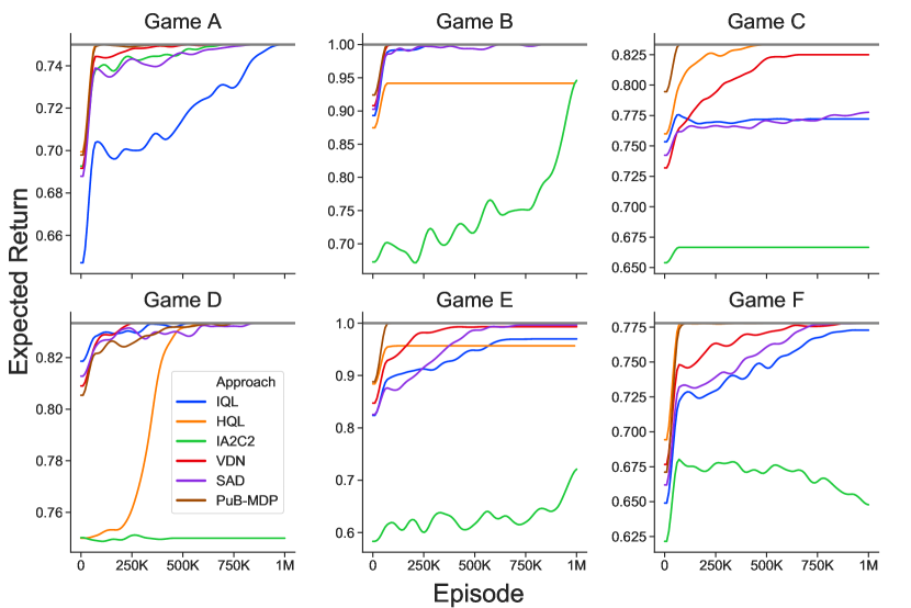
Figure 3: Performance comparison in the Tiny Hanabi Suite. Q-learning in the PuB-MDP consistently solves every game. In contrast, the algorithms operating within the independent reinforcement learning paradigm (IQL, HQL, IA2C2, VDN, SAD) are unable to do so.

Algorithm 1 CAPI

procedure act($b$, $K$)

     $[\Gamma^{(k)}]\leftarrow\mbox{prescription\_vectors}(\pi(b),K)$

     $[r^{(k)}]\leftarrow\mbox{expected\_rewards}(b,[\Gamma^{(k)}])$

     $[b^{(k,O_{\mbox{pub}})}]\leftarrow\mbox{next\_beliefs}(b,[\Gamma^{(k)}])$

     $[v^{(k,O_{\mbox{pub}})}]\leftarrow\mbox{estimate\_values}([b^{(k,O_{\mbox{pub}})}])$

     $[p^{(k)}]\leftarrow\mbox{pub\_observation\_probabilities}(b,[\Gamma^{(k)}])$

     $[q^{(k)}]\leftarrow[r^{(k)}]+\mbox{pub\_expectation}([p^{(k)}],[v^{(k,O_{\mbox{pub}})}])$

     $k^{\ast}\leftarrow\mbox{argmax}([q^{(k)}])$

     $\mbox{add\_to\_buffer}(b,\Gamma^{(k^{\ast})},q^{(k^{\ast})})$

     if explore then

         return $\mbox{random}([\Gamma^{(k)}])$      

     return $\Gamma^{(k^{\ast})}$

We run CAPI without sampling transitions, meaning that the episode is played out for every transition (i.e., every branch of the public tree) that occurs with positive probability, rather than sampling each transition. After each episode, we train the value network and policy and wipe the buffer.

As of yet, we have left two important details unexplained. First, how can CAPI pass a belief state over an exponential number of histories into a network? To do so, CAPI adopts a trick from DeepStack (Moravčík, Schmid et al. 2017; Kovarík and Lisý 2019), and instead passes the public state $s$ and each player’s contribution to the reach probability

$$\left[P^{\pi}_{i}|_{\mathcal{S}_{i}(s)}(\cdot\mid s)\right]_{i\in\mathcal{N}}$$

as input, where $P^{\pi}_{i}$ denotes player $i$’s contribution to the reach probability and $f\mid_{X}$ denotes the function $f$ restricted to the domain $X$. This information is a sufficient statistic for the belief state, but is more compact (albeit still exponential in the general case). An explanation of sufficiency is offered in the appendix and can also be found in Kovarík and Lisý.

Second, how can CAPI maintain a policy over an exponentially large space? To do so, CAPI adopts a trick from BAD (Foerster et al. 2019) and uses a distribution over prescription vectors that factors across information states

$$P(\Gamma\mid b)=\prod_{i\in\mathcal{N}}\prod_{s_{i}\in\mathcal{S}_{i}(b)}\pi(\Gamma(s_{i})\mid b).$$

This parameterization reduces the space required to store the distribution from $|\mathcal{A}_{i}|^{N\cdot|\mathcal{S}_{i}|}$ to $|\mathcal{A}_{i}|\cdot N\cdot|\mathcal{S}_{i}|$, making it explicitly manageable in the games we consider. While this parameterization is constraining in that direct optimization by gradient ascent will only guarantee a local optima, search gives CAPI the opportunity to escape these local optima. CAPI can optionally exploit this parameterization to add structured exploration by randomly setting rows of the policy to uniform random.

Experiments

Problem Domains

We consider two common-payoff games from OpenSpiel (Lanctot, Lockhart et al. 2019) to demonstrate the efficacy of CAPI.

Trade Comm

The first is a communication game based on trading called Trade Comm. The game proceeds as follows.

1. Each player is independently dealt one of num_items with uniform chance.

2. Player 1 makes one of num_utterances utterances, which is observed by player 2.

3. Player 2 makes one of num_utterances utterances, which is observed by player 1.

4. Both players privately request one of the $\texttt{num\_items}*\texttt{num\_items}$ possible trades.

The trade is successful if and only if both player 1 asks to trade its item for player 2’s item and player 2 asks to trade its item for player 1’s item. Both players receive a reward of one if the trade is successful and zero otherwise. In our experiment, we use $\texttt{num\_items}=\texttt{num\_utterances}=12$. This means that there is exactly enough bandwidth for the players to losslessly communicate their items and an optimal policy receives an expected reward of one.

This deceivingly easy-sounding game nicely illustrates the difficulty of common-payoff games. It is too large to be tackled directly by using a public POMDP transformation and POMDP solution methods (the combination of which have been applied to games having fewer than 10 actions, whereas Trade Comm has 100s). But simultaneously, as is shown in the appendix, independent deep reinforcement learning (Mnih, Kavukcuoglu et al. 2015; Mnih et al. 2016) catastrophically fails to learn a good policy.

The code used to generate the results for CAPI is available at https://github.com/ssokota/capi.

Abstracted Tiny Bridge

For our second game, we consider Abstracted Tiny Bridge, which is a small common-payoff version of contract bridge retaining some interesting strategic elements. In the game, each player is dealt one of 12 hands as a private observation. The two players then bid to choose the contract. The common payoff is determined by the chosen contract, the hand of the player who chose the contract, and the hand of player who did not chose the contract. The challenge of the game is that the players must use their bids (actions) both to signal their hands and to select the contract, for which there are increasingly limited options as more bids are made. The exact rules are detailed on OpenSpiel.

Despite its name, Abstracted Tiny Bridge is much larger than games traditionally considered in Dec-POMDP literature, having over 50,000 nonterminal Markov states. For reference, Mars Rover (Amato and Zilberstein 2009), the largest game considered by many Dec-POMDP papers, has only 256.

Baselines

We again use tabular IQL, HQL, IA2C2, VDN, and SAD as baselines. In our preliminary experiments the tabular implementations of these algorithms outperformed the respective deep variants.

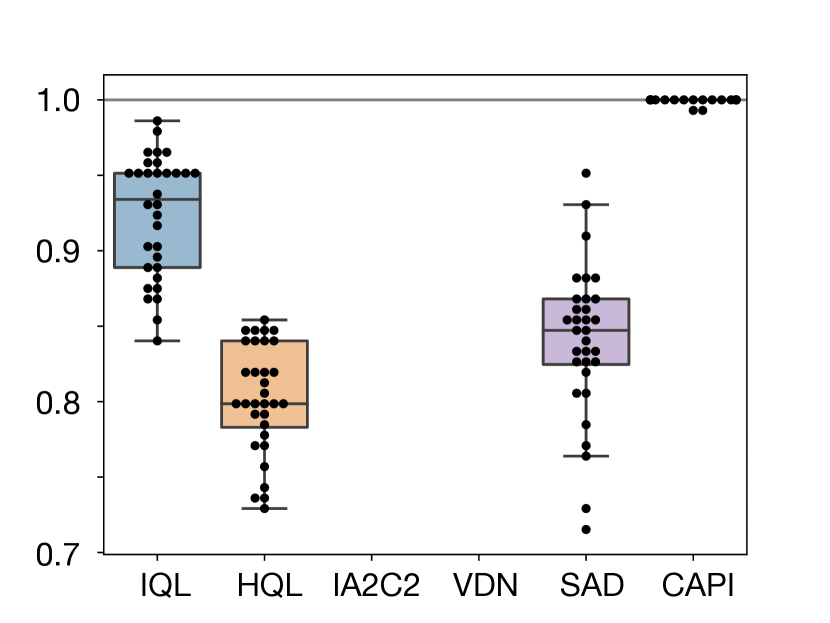
Figure 4: Performance comparison in Trade Comm. CAPI consistently solves the game (30/32), whereas none of IQL, HQL, IA2C2, VDN, or SAD found an optimal policy on any of the 32 runs. Results for IA2C2 and VDN are below the bottom cutoff of the graph. Reported results are for best joint policy discovered.

Results

Below, we describe the high level takeaways of our experiments. Implementation details can be found in the appendix.

Trade Comm

In Figure 4, we show results for IQL, HQL, IA2C2, VDN, and SAD after 24 hours (as many as 100 million episodes) and results for CAPI after 2,000 episodes. To give context to the scores on the graph, the optimal return is one (gray line) and the best joint policies that do not require coordination achieve an expected return of only 1/144. IA2C2 and VDN (below bottom cutoff of graph) barely outperformed the best no-coordination joint policy. The poor performance for IA2C2 may be attributable to the stochasticity of its policies, which are not well suited to Trade Comm’s sparse rewards. For VDN, the poor performance may be caused by its assumption that the joint value function decomposes additively, which provides a bad inductive bias for Trade Comm’s non-monotonic value landscape. In contrast to IA2C2 and VDN, HQL, IQL, SAD, and CAPI significantly outperform the best no-coordination joint policies. Among the three, CAPI does the best, solving the game in 30 out of the 32 runs and nearly solving it on the remaining 2. In contrast, none of IQL, HQL, and SAD solve Trade Comm on any of their respective 32 runs.

Abtracted Tiny Bridge

In Figure 5, we show results for IQL, HQL, IA2C2, VDN, and SAD after 10 million episodes and results for CAPI after 100 thousand episodes. To give context to the scores on the graph, the optimal return is the gray line and the best joint policy that we are aware of that does not require coordination achieves an expected return of 20.32. IA2C2 arguably performed the worst, having both the lowest scoring minimum, median and maximum. IQL and VDN performed comparably, with VDN performing slightly worse. HQL and SAD arguably performed the best among the independent reinforcement learning algorithms, consistently discovering policies that outperform the others on average. CAPI shows the strongest performance, solving the game on 18 of its 32 runs, contrasting the independent reinforcement learning algorithms, which do not solve the game on any of their runs and perform significantly worse on average.

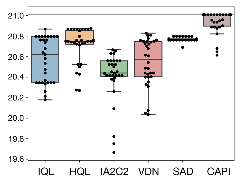
Figure 5: Performance comparison in Abstracted Tiny Bridge. CAPI solves the game on 18 of the 32 runs. None of IQL, HQL, IA2C2, VDN, or SAD solve the game on any of their respective runs. Reported results are for best joint policy discovered.

Related Work

From Dec-POMDP Literature

Independently from Nayyar, Mahajan, and Teneketzis, Dibangoye et al. (Dibangoye et al. 2016) show that a common-payoff game can be converted into a non-observable MDP (NOMDP) (Oliehoek and Amato 2014), a special kind of POMDP in which the agent (in this case the coordinator) receives no observations. Dibangoye et al. call the corresponding belief MDP the occupancy state MDP. Dibangoye et al. also introduce feature-based heuristic search value iteration (FB-HSVI), a novel planning algorithm with asymptotic optimality guarantees. In a large-scale study, Dibangoye et al. show that combining the occupancy state, FB-HSVI, and equivalence relations over information states is able to solve games with hundreds of states and outperforms contemporaneously existing methods.

MacDermed and Isbell build on the occupancy state MDP approach, showing that it can be extended to infinite horizon problems when beliefs are bounded. They also show how belief compression can be combined with point-based value iteration (Spaan and Vlassis 2005) to achieve good empirical results. There is also recent work that extends the occupancy state MDP approach to the reinforcement learning problem setting (Dibangoye and Buffet 2018) and to special cases involving asymmetric observability (Xie, Dibangoye, and Buffet 2020).

Compared to the games investigated in these works, the games investigated in this work are larger. However, the scalability that is gained by leveraging deep learning and CAPI’s policy parameterization precludes CAPI from having the same guarantees as these algorithms.

From Cooperative MARL Literature

Outside of this work, there has also been work by the multi-agent reinforcement learning community to apply the PuB-MDP at scale. BAD (Foerster et al. 2019) scales a policy-based approach to the PuB-MDP by using an independence assumption across private features to analytically approximate belief states and an independence assumption to parameterize the distribution over prescription vectors. Foerster et al. also introduce a belief update correction procedure resembling expectation propagation (Minka 2001) and use population-based training to show how BAD can be scaled to two-player Hanabi.

Compared to BAD, CAPI is significantly less scalable—two-player Hanabi is much larger than the games considered in this work. However, the cost of this scalability is that BAD cannot solve games even as small as game E of the Tiny Hanabi Suite. In contrast, our results demonstrate that CAPI is capable of discovering optimal policies.

There has also been work applying decision-time search at scale in common-payoff games. SPARTA (Lerer et al. 2020) runs a one-ply search over the next action in the game at each public belief state, using an externally specified policy as a blueprint according to which the rest of the rollout is played. Lerer et al. show that in the limit in the number of rollouts, SPARTA produces a policy no worse than its blueprint. In practice, empirical results on Hanabi suggest that SPARTA’s policy tends to significantly outperform its blueprint.

Similarly to SPARTA, CAPI performs decision-time planning in the PuB-MDP. Unlike SPARTA, CAPI is a self-contained learning algorithm and does not require an externally specified blueprint. It is also unlike SPARTA in that its design principles are geared toward solving games, whereas SPARTA is designed for scalability and has failure cases even in small games.

From Adversarial Game Literature

Public belief states have also played an important role in recent successes in adversarial games. In poker, DeepStack (Moravčík, Schmid et al. 2017), Libratus (Brown and Sandholm 2018), and Pluribus (Brown and Sandholm 2019) combine public belief states (Brown and Sandholm 2017; Šustr, Kovařík, and Lisý 2019) with equilibrium computation methods and precomputed value functions (Kovarík and Lisý 2019). More recently, Brown et al. proposed ReBeL (Brown et al. 2020), which is similar to CAPI in that both learn policies and value functions over public belief states from self-play and use decision-time planning.

From Mixed-Motive Game Literature

Recent work on the game Diplomacy is similar to CAPI in how it handles a combinatorial action space (Anthony, Eccles et al. 2020; Gray, Lerer et al. 2020). The sampled best response algorithm Anthony, Eccles et al. propose is especially similar in that it also performs a one-ply search using a variant of policy iteration with sampled actions. The equilibrium search algorithm Gray, Lerer et al. propose is also similar in that it performs a one-ply search over the $K$-most-likely actions.

Conclusion and Future Work

In this work, inspired by BAD (Foerster et al. 2019) and the seminal work of Nayyar, Mahajan, and Teneketzis, we propose CAPI, a novel approximate policy iteration algorithm for common-payoff imperfect information games. In many ways, CAPI is similar to BAD, but differs notably in that it is more correct and less scalable. Empirically, we demonstrate the efficacy of CAPI by showing that it is able to solve games on which modern multi-agent reinforcement learning algorithms struggle.

The direction for future work that we are most interested in is the construction of a single public knowledge approach inheriting CAPI’s performance (or better) on small games and BAD’s performance (or better) on large games. The existence of such an algorithm would be an exciting and unifying discovery. It may require effective mechanisms for learning or approximating public belief states and for working with compressed or implicit representations of prescription vectors. Both of these mechanisms would also be of significance for two-player zero-sum games, where the intractability of public belief states and prescription vectors is a limiting factor for applying decision-time planning approaches to larger problems.

Compact Belief Factorization

In general, the size of the public set grows exponentially in time. Even assuming that the public set is small enough to keep a posterior over, this posterior may still be too unwieldy for practical use as input to a value or policy network. By exploiting playerwise factorization, we can produce a sufficient statistic that, while still growing exponentially, is much smaller than the posterior over histories (Moravčík, Schmid et al. 2017; Kovarík and Lisý 2019). Observe that the publicly conditioned probability of any history can be expanded as

$$P^{\pi}(h\mid s)=\frac{P_{\mathcal{T}}(h)\prod_{i=1}^{N}P^{\pi}_{i}(s_{i}(h))}{\sum_{h^{\prime}\in I_{\mbox{pub}}(s)}P_{\mathcal{T}}(h^{\prime})\prod_{i=1}^{N}P^{\pi}_{i}(s_{i}(h^{\prime}))}.$$

It follows that the publicly conditioned posterior over histories can be losslessly reconstructed from the public state and each player’s contribution function by a mapping of the form

$$\left[s,P^{\pi}_{1}|_{\mathcal{S}_{1}(s)}(\cdot\mid s),\dots,P^{\pi}_{N}|_{\mathcal{S}_{N}(s)}(\cdot\mid s)\right]\longmapsto P^{\pi}|_{I_{\mbox{pub}}(s)}(\cdot\mid s)$$

that is independent of the historical policy profile. Therefore, the input of this mapping is a sufficient to estimate the public belief state value. While this statistic still grows exponentially in the length of the game, it is a much smaller dimensionality than the posterior over histories and it grows only linearly in the number players.

Independent Deep Reinforcement Learning for Trade Comm

To emphasize the difficulty of Trade Comm, we ran a hyperparameter sweep for independent DQN and A2C. The DQN agents were trained with all combinations of following parameters: learning rate $[2e-1,1e-1,1e-2,1e-3,1e-4]$, decaying exploration starting at $[1.,0.8,0.5,0.2]$, hidden layer size of {’64’, ’128’, ’32, 32’, ’64, 64’} and replay buffer capacity of $[50,100,1000,10000]$. The A2C agents were trained with all combinations of following parameters: critic learning rate $[1e-2,1e-3]$, actor learning rate $[1e-3,1e-4,1e-5]$, number of critic updates before every actor update $[4,8,16]$ and hidden-layer size of {’32’, ’64’, ’128’, ’32, 32’, ’64, 64’}. Both the independent DQN agents and the independent A2C agents were trained for $5e{+}6$ steps. We ran 3 runs at each parameter setting. In total the parameter sweep took 45 hours and 14 minutes.

We trained both the independent DQN agents and the independent A2C agents to play a version of Trade Comm with 10 items and 10 utterances. The best DQN agents achieved an expected return of around 0.12. No A2C agents achieved an expected return of more than 0.01.

Implementation Details

IQL, HQL, IA2C2, VDN, SAD

We used a linearly decaying epsilon and a linearly decaying learning rate for both games.

Trade Comm

For Trade Comm, the rate of decay was set such that both the epsilon value and the learning rate value would reach zero after 100 million episodes. To determine the initial values, we did a grid search over the values $[0.1,0.2,0.3,0.4,0.5]$ for the initial epsilon and $[0.1,0.2,0.3,0.4,0.5]$ for the initial learning rate.

Abstracted Tiny Bridge

For Abstracted Tiny Bridge, the rate of decay was set such that both the epsilon value and the learning rate value would reach zero after 10 million episodes. We did a grid search over the values $[0.1,0.2,0.3]$ for the initial epsilon and $[0.05,0.1,0.2]$ for the initial learning rate.

CAPI

In both games we used 3 layer neural network with 256 units per hidden layer and the Adam optimizer for the value function.

Trade Comm

For Trade Comm we used a two-headed network to produce the value and policy, randomly sampled 10,000 prescription vectors from the policy, and used $\epsilon$-greedy exploration with $\epsilon=0.1$. We used a learning rate of $1e-4$, a weight of 1/100 for the loss of the policy head and a weight of 1 for that of the value head. We used mean squared error for the value head and cross entropy loss for the policy head.

Abstracted Tiny Bridge

For Abstracted Tiny Bridge we maintained a tabular policy for each public state, added structured exploration by overwriting a random row of the policy to be uniformly random during training, generated the 10,000 most likely prescription vectors from the policy, and played an exploratory prescription vector once an episode.

For the policy we used a learning rate of $1e{-}6$ and a floor of 0.01. We explored once every episode. We also added structured exploration by setting a row of the prescription vector to uniform random at each decision point. We squashed the output of the value network to be between -1 and 1 by applying sigmoid to the output. We used a mean squared error loss for the value network.

The Tiny Hanabi Suite

The Tiny Hanabi Suite is a collection of six toy common-payoff games created by Neil Burch and Nolan Bard. Each game is structured in three steps.

1. A dealer samples two cards from separate piles of num_cards cards with uniform probability and gives the first card to player one and the second player two.

2. Player one chooses one of num_actions actions. Player two observes player one’s action.

3. Player two chooses one of num_actions actions.

After player two’s action, the game ends and the common payoff is determined as a function of the cards dealt and the actions taken.

Although the tiny Hanabi games are most naturally thought of as temporally-extended, the payoff functions can be succinctly described as payoff tables, as is shown in Figure 6, Figure 7, Figure 8, Figure 9, Figure 10, and Figure 11.

• The uppercase numerals in the leftmost column represent the card dealt to player one.

• The lowercase numerals in the uppermost column represent the card dealt to player two.

• The uppercase letters represent player one’s action.

• The lowercase letters represent player two’s action.

• The integer corresponding to a particular quadruplet is the payoff to that trajectory.

In games A, B, C, and D, num_cards$=2$ and num_actions$=2$. In game E, num_cards$=2$ and num_actions$=3$. In game F, num_cards$=3$ and num_actions$=2$.

Game A

Card		i		ii
	Action	a	b	a	b
I	A	0	1	0	1
	B	0	0	3	2
II	A	3	3	2	0
	B	3	2	3	3

Figure 6: Game A of the Tiny Hanabi Suite.

Game B

Card		i		ii
	Action	a	b	a	b
I	A	1	0	0	1
	B	1	0	0	1
II	A	0	1	1	0
	B	0	0	1	0

Figure 7: Game B of the Tiny Hanabi Suite.

Game C

Card		i		ii
	Action	a	b	a	b
I	A	3	0	2	0
	B	0	3	3	3
II	A	2	2	0	1
	B	3	0	0	2

Figure 8: Game C of the Tiny Hanabi Suite.

Game D

Card		i		ii
	Action	a	b	a	b
I	A	3	0	3	0
	B	1	3	3	0
II	A	3	2	0	1
	B	0	2	0	0

Figure 9: Game D of the Tiny Hanabi Suite.

Game E

Card		i			ii
	Action	a	b	c	a	b	c
I	A	10	0	0	0	0	10
	B	4	8	4	4	8	4
	C	10	0	0	0	0	10
II	A	0	0	10	10	0	0
	B	4	8	4	4	8	4
	C	0	0	0	10	0	0

Figure 10: Game E of the Tiny Hanabi Suite.

Game F

Card		i		ii		iii
	Action	a	b	a	b	a	b
I	A	0	3	0	0	3	1
	B	3	2	0	1	2	1
II	A	0	2	1	2	0	1
	B	0	1	1	2	0	3
III	A	1	3	0	3	3	1
	B	1	2	2	2	3	0

Figure 11: Game F of the Tiny Hanabi Suite.

References

- Afshari and Mahajan (2018) Afshari, M.; and Mahajan, A. 2018. Team Optimal Decentralized State Estimation. 2018 IEEE Conference on Decision and Control (CDC) 5044–5050.
- Amato and Zilberstein (2009) Amato, C.; and Zilberstein, S. 2009. Achieving Goals in Decentralized POMDPs. In Proceedings of The 8th International Conference on Autonomous Agents and Multiagent Systems - Volume 1, AAMAS ’09. International Foundation for Autonomous Agents and Multiagent Systems.
- Anthony, Eccles et al. (2020) Anthony, T.; Eccles, T.; et al. 2020. Learning to Play No-Press Diplomacy with Best Response Policy Iteration.
- Arabneydi and Mahajan (2014) Arabneydi, J.; and Mahajan, A. 2014. Team optimal control of coupled subsystems with mean-field sharing. In 53rd IEEE Conference on Decision and Control, 1669–1674.
- Arabneydi and Mahajan (2015) Arabneydi, J.; and Mahajan, A. 2015. Reinforcement learning in decentralized stochastic control systems with partial history sharing. In 2015 American Control Conference (ACC), 5449–5456. doi:10.1109/ACC.2015.7172192.
- Aumann (1976) Aumann, R. 1976. Agreeing to disagree. The Annals of Statistics 4(6): 1236–1239.
- Bernstein et al. (2000) Bernstein, D. S.; Givan, R.; Immerman, N.; and Zilberstein, S. 2000. The Complexity of Decentralized Control of Markov Decision Processes. Math. Oper. Res. 27: 819–840.
- Bono et al. (2018) Bono, G.; Dibangoye, J. S.; Matignon, L.; Pereyron, F.; and Simonin, O. 2018. Cooperative Multi-agent Policy Gradient. In ECML/PKDD (1).
- Brown et al. (2020) Brown, N.; Bakhtin, A.; Lerer, A.; and Gong, Q. 2020. Combining Deep Reinforcement Learning and Search for Imperfect-Information Games.
- Brown and Sandholm (2017) Brown, N.; and Sandholm, T. 2017. Safe and Nested Subgame Solving for Imperfect-Information Games. In Advances in Neural Information Processing Systems 30.
- Brown and Sandholm (2018) Brown, N.; and Sandholm, T. 2018. Superhuman AI for heads-up no-limit poker: Libratus beats top professionals. Science 359: 418–424.
- Brown and Sandholm (2019) Brown, N.; and Sandholm, T. 2019. Superhuman AI for multiplayer poker. Science .
- Clark and Marshall (1981) Clark, H. H.; and Marshall, C. R. 1981. Definite Knowledge and Mutual Knowledge. In Elements of Discourse Understanding.
- Claus and Boutilier (1998) Claus, C.; and Boutilier, C. 1998. The Dynamics of Reinforcement Learning in Cooperative Multiagent Systems. In Proceedings of the Fifteenth National/Tenth Conference on Artificial Intelligence/Innovative Applications of Artificial Intelligence. American Association for Artificial Intelligence.
- Dibangoye et al. (2016) Dibangoye, J. S.; Amato, C.; Buffet, O.; and Charpillet, F. 2016. Optimally Solving Dec-POMDPs As Continuous-state MDPs. J. Artif. Int. Res. 55(1): 443–497.
- Dibangoye and Buffet (2018) Dibangoye, J. S.; and Buffet, O. 2018. Learning to Act in Decentralized Partially Observable MDPs. In Dy, J. G.; and Krause, A., eds., Proceedings of the 35th International Conference on Machine Learning, ICML 2018.
- Foerster et al. (2017) Foerster, J.; Farquhar, G.; Afouras, T.; Nardelli, N.; and Whiteson, S. 2017. Counterfactual Multi-Agent Policy Gradients.
- Foerster et al. (2019) Foerster, J.; Song, F.; Hughes, E.; et al. 2019. Bayesian Action Decoder for Deep Multi-Agent Reinforcement Learning. In Proceedings of the 36th International Conference on Machine Learning, Proceedings of Machine Learning Research, 1942–1951. Long Beach, California, USA: PMLR.
- Gagrani and Nayyar (2017) Gagrani, M.; and Nayyar, A. 2017. Decentralized minimax control problems with partial history sharing. In 2017 American Control Conference (ACC), 3373–3379.
- Gagrani and Nayyar (2018) Gagrani, M.; and Nayyar, A. 2018. Thompson Sampling for some decentralized control problems. 2018 IEEE Conference on Decision and Control (CDC) 1053–1058.
- Gray, Lerer et al. (2020) Gray, J.; Lerer, A.; et al. 2020. Human-Level Performance in No-Press Diplomacy via Equilibrium Search.
- Gupta (2020) Gupta, A. 2020. Existence of Team-Optimal Strategies in Teams with Countable Observation Spaces. IEEE Transactions on Automatic Control 1–1.
- Hadfield-Menell et al. (2016) Hadfield-Menell, D.; Russell, S. J.; Abbeel, P.; and Dragan, A. 2016. Cooperative Inverse Reinforcement Learning. In Advances in Neural Information Processing Systems 29.
- Halpern and Moses (2000) Halpern, J. Y.; and Moses, Y. 2000. Knowledge and common knowledge in a distributed environment. CoRR cs.DC/0006009. URL http://arxiv.org/abs/cs.DC/0006009.
- Hausknecht and Stone (2015) Hausknecht, M. J.; and Stone, P. 2015. Deep Recurrent Q-Learning for Partially Observable MDPs. In AAAI Fall Symposia.
- Hu and Foerster (2020) Hu, H.; and Foerster, J. N. 2020. Simplified Action Decoder for Deep Multi-Agent Reinforcement Learning. In International Conference on Learning Representations.
- Kovarík and Lisý (2019) Kovarík, V.; and Lisý, V. 2019. Value Functions for Depth-Limited Solving in Zero-Sum Imperfect-Information Games. CoRR abs/1906.06412.
- Kovarík et al. (2019) Kovarík, V.; Schmid, M.; Burch, N.; Bowling, M.; and Lisý, V. 2019. Rethinking Formal Models of Partially Observable Multiagent Decision Making. CoRR abs/1906.11110.
- Lanctot, Lockhart et al. (2019) Lanctot, M.; Lockhart, E.; et al. 2019. OpenSpiel: A Framework for Reinforcement Learning in Games.
- Lazaridou, Peysakhovich, and Baroni (2017) Lazaridou, A.; Peysakhovich, A.; and Baroni, M. 2017. Multi-Agent Cooperation and the Emergence of (Natural) Language. ArXiv abs/1612.07182.
- Lerer et al. (2020) Lerer, A.; Hu, H.; Foerster, J. N.; and Brown, N. 2020. Improving Policies via Search in Cooperative Partially Observable Games. In AAAI.
- Lessard and Nayyar (2013) Lessard, L.; and Nayyar, A. 2013. Structural results and explicit solution for two-player LQG systems on a finite time horizon. In 52nd IEEE Conference on Decision and Control.
- Lewis (1969) Lewis, D. K. 1969. Convention: A Philosophical Study. Wiley-Blackwell.
- Leyton-Brown and Shoham (2008) Leyton-Brown, K.; and Shoham, Y. 2008. Essentials of Game Theory: A Concise, Multidisciplinary Introduction. Morgan and Claypool Publishers, 1st edition.
- Littman (1994) Littman, M. L. 1994. Markov Games as a Framework for Multi-Agent Reinforcement Learning. In ICML.
- Lowe et al. (2017) Lowe, R.; Wu, Y.; Tamar, A.; Harb, J.; Abbeel, P.; and Mordatch, I. 2017. Multi-Agent Actor-Critic for Mixed Cooperative-Competitive Environments.
- MacDermed and Isbell (2013) MacDermed, L. C.; and Isbell, C. L. 2013. Point Based Value Iteration with Optimal Belief Compression for Dec-POMDPs. In Advances in Neural Information Processing Systems 26.
- Matignon, Laurent, and Le Fort-Piat (2007) Matignon, L.; Laurent, G. J.; and Le Fort-Piat, N. 2007. Hysteretic Q-learning : an algorithm for Decentralized Reinforcement Learning in Cooperative Multi-Agent Teams. In 2007 IEEE/RSJ International Conference on Intelligent Robots and Systems, 64–69.
- Minka (2001) Minka, T. P. 2001. Expectation Propagation for Approximate Bayesian Inference. In Proceedings of the Seventeenth Conference on Uncertainty in Artificial Intelligence.
- Mnih, Kavukcuoglu et al. (2015) Mnih, V.; Kavukcuoglu, K.; et al. 2015. Human-level control through deep reinforcement learning. Nature 518(7540): 529–533. ISSN 00280836.
- Mnih et al. (2016) Mnih, V.; et al. 2016. Asynchronous Methods for Deep Reinforcement Learning. In Proceedings of The 33rd International Conference on Machine Learning, Proceedings of Machine Learning Research, 1928–1937. PMLR.
- Moravčík, Schmid et al. (2017) Moravčík, M.; Schmid, M.; et al. 2017. DeepStack: Expert-level artificial intelligence in heads-up no-limit poker. Science 356(6337): 508–513.
- Nair et al. (2003) Nair, R.; et al. 2003. Taming Decentralized POMDPs: Towards Efficient Policy Computation for Multiagent Settings. In Proceedings of the 18th International Joint Conference on Artificial Intelligence, IJCAI’03, 705–711.
- Nayyar et al. (2014) Nayyar, A.; Gupta, A.; Langbort, C.; and Başar, T. 2014. Common Information Based Markov Perfect Equilibria for Stochastic Games With Asymmetric Information: Finite Games. IEEE Transactions on Automatic Control .