Abstract

We obtain global, non-asymptotic convergence guarantees for independent learning algorithms in competitive reinforcement learning settings with two agents (i.e., zero-sum stochastic games). We consider an episodic setting where in each episode, each player independently selects a policy and observes only their own actions and rewards, along with the state. We show that if both players run policy gradient methods in tandem, their policies will converge to a min-max equilibrium of the game, as long as their learning rates follow a two-timescale rule (which is necessary). To the best of our knowledge, this constitutes the first finite-sample convergence result for independent policy gradient methods in competitive RL; prior work has largely focused on centralized, coordinated procedures for equilibrium computation.

1 Introduction

Reinforcement learning (RL)—in which an agent must learn to maximize reward in an unknown dynamic environment—is an important frontier for artificial intelligence research, and has shown great promise in application domains ranging from robotics (Kober et al., 2013; Lillicrap et al., 2015; Levine et al., 2016) to games such as Atari, Go, and Starcraft (Mnih et al., 2015; Silver et al., 2017; Vinyals et al., 2019). Many of the most exciting recent applications of RL are game-theoretic in nature, with multiple agents competing for shared resources or cooperating to solve a common task in stateful environments where agents’ actions influence both the state and other agents’ rewards (Silver et al., 2017; OpenAI, 2018; Vinyals et al., 2019). Algorithms for such multi-agent reinforcement learning (MARL) settings must be capable of accounting for other learning agents in their environment, and must choose their actions in anticipation of the behavior of these agents. Developing efficient, reliable techniques for MARL is a crucial step toward building autonomous and robust learning agents.

While single-player (or, non-competitive RL has seen much recent theoretical activity, including development of efficient algorithms with provable, non-asymptotic guarantees (Dann and Brunskill, 2015; Azar et al., 2017; Jin et al., 2018; Dean et al., 2019; Agarwal et al., 2020), provable guarantees for MARL have been comparatively sparse. Existing algorithms for MARL can be classified into centralized/coordinated algorithms and independent/decoupled algorithms (Zhang et al., 2019a). Centralized algorithms such as self-play assume the existence of a centralized controller that joinly optimizes with respect to all agents’ policies. These algorithms are typically employed in settings where the number of players and the type of interaction (competitive, cooperative, etc.) are both known a-priori. On the other hand, in independent reinforcement learning, agents behave myopically and optimize their own policy while treating the environment as fixed. They observe only local information, such as their own actions, rewards, and the part of the state that is available to them. As such, independent learning algorithms are generally more versatile, as they can be applied even in uncertain environments where the type of interaction and number of other agents are not known to the individual learners.

Both centralized (Silver et al., 2017; OpenAI, 2018; Vinyals et al., 2019) and independent (Matignon et al., 2012; Foerster et al., 2017) algorithms have enjoyed practical success across different domains. However, while centralized algorithms have experienced recent theoretical development, including provable finite-sample guarantees (Wei et al., 2017; Bai and Jin, 2020; Xie et al., 2020), theoretical guarantees for independent reinforcement learning have remained elusive. In fact, it is known that independent algorithms may fail to converge even in simple multi-agent tasks (Condon, 1990; Tan, 1993; Claus and Boutilier, 1998): When agents update their policies independently, they induce distribution shift, which can break assumptions made by classical single-player algorithms. Understanding when these algorithms work, and how to stabilize their performance and tackle distribution shift, is recognized as a major challenge in multi-agent RL (Matignon et al., 2012; Hernandez-Leal et al., 2017).

In this paper, we focus on understanding the convergence properties of independent reinforcement learning with policy gradient methods (Williams, 1992; Sutton et al., 2000). Policy gradient methods form the foundation for modern applications of multi-agent reinforcement learning, with state-of-the-art performance across many domains (Schulman et al., 2015, 2017). Policy gradient methods are especially relevant for continuous reinforcement learning and control tasks, since they readily scale to large action spaces, and are often more stable than value-based methods, particularly with function approximation (Konda and Tsitsiklis, 2000). Independent reinforcement learning with policy gradient methods is poorly understood, and attaining global convergence results is considered an important open problem (Zhang et al., 2019a, Section 6).

We analyze the behavior of independent policy gradient methods in Shapley’s stochastic game framework (Shapley, 1953). We focus on two-player zero-sum stochastic games with discrete state and action spaces, wherein players observe the entire joint state, take simultaneous actions, and observe rewards simultaneously, with one player trying to maximize the reward and the other trying to minimize it. To capture the challenge of independent learning, we assume that each player observes the state, reward, and their own action, but not the action chosen by the other player. We assume that the dynamics and reward distribution are unknown, so that players must optimize their policies using only realized trajectories consisting of the states, rewards, and actions. For this setting, we show that—while independent policy gradient methods may not converge in general—policy gradient methods following a two-timescale rule converge to a Nash equilibrium. We also show that moving beyond two-timescale rules by incorporating optimization techniques from matrix games such as optimism (Daskalakis et al., 2017) or extragradient updates (Korpelevich, 1976) is likely to require new analysis techniques.

At a technical level, our result is a special case of a more general theorem, which shows that (stochastic) two-timescale updates converge to Nash equilibria for a class of nonconvex minimax problems satisfying a certain two-sided gradient dominance property. Our results here expand the class of nonconvex minimax problems with provable algorithms beyond the scope of prior work (Yang et al., 2020), and may be of independent interest.

2 Preliminaries

We investigate the behavior of independent learning in two-player zero-sum stochastic games (or, Markov games), a simple competitive reinforcement learning setting (Shapley, 1953; Littman, 1994). In these games, two players—a min-player and a max-player—repeatedly select actions simultaneously in a shared Markov decision process in order to minimize and maximize, respectively, a given objective function. Formally, a two-player zero-sum stochastic game is specified by a tuple $\mathcal{G}=(\mathcal{S},\mathcal{A},\mathcal{B},P,R,\zeta,\rho)$:

• $\mathcal{S}$ is a finite state space of size $S=|\mathcal{S}|$.

• $\mathcal{A}$ and $\mathcal{B}$ are finite action spaces for the min- and max-players, of sizes $A=|\mathcal{A}|$ and $B=|\mathcal{B}|$.

• $P$ is the transition probability function, for which $P(s^{\prime}\mid s,a,b)$ denotes the probability of transitioning to state $s^{\prime}$ when the current state is $s$ and the players take actions $a$ and $b$. In general we will have $\zeta_{s,a,b}\vcentcolon={}1-\sum_{s^{\prime}\in\mathcal{S}}P(s^{\prime}\mid s,a,b)>0$; this quantity represents the probability that $\mathcal{G}$ stops at state $s$ if actions $a,b$ are played.

• $R:\mathcal{S}\times\mathcal{A}\times\mathcal{B}\rightarrow[-1,1]$ is the reward function; $R(s,a,b)$ gives the immediate reward when the players take actions $a,b$ in state $s$. The min-player seeks to minimize $R$ and the max-player seeks to maximize it.

• $\zeta:=\min_{s,a,b}\{\zeta_{s,a,b}\}$ is a lower bound on the probability that the game stops at any state $s$ and choices of actions $a,b$. We assume that $\zeta>0$ throughout this paper.

• $\rho\in\Delta(\mathcal{S})$ is the initial distribution of the state at time $t=0$.

At each time step $t\geq 0$, both players observe a state $s_{t}\in\mathcal{S}$, pick actions $a_{t}\in\mathcal{A}$ and $b_{t}\in\mathcal{B}$, receive reward $r_{t}\vcentcolon={}R(s_{t},a_{t},b_{t})$, and transition to the next state $s_{t+1}\sim P(\cdot\mid s_{t},a_{t},b_{t})$. With probability $\zeta_{s_{t},a_{t},b_{t}}$, the game stops at time $t$; since $\zeta>0$, the game stops eventually with probability $1$.

A pair of (randomized) policies $\pi_{1}:\mathcal{S}\to\Delta(\mathcal{A})$, $\pi_{2}:\mathcal{S}\to\Delta(\mathcal{B})$ induces a distribution $\operatorname{Pr}^{\pi_{1},\pi_{2}}$ of trajectories $(s_{t},a_{t},b_{t},r_{t})_{0\leq t\leq T}$, where $s_{0}\sim\rho$, $a_{t}\sim\pi_{1}(\cdot\mid s_{t}),b_{t}\sim\pi_{2}(\cdot\mid s_{t})$, $r_{t}=R(s_{t},a_{t},b_{t})$, and $T$ is the last time step before the game stops (which is a random variable). The value function $V_{s}(\pi_{1},\pi_{2})$ gives the expected reward when $s_{0}=s$ and the plays follow $\pi_{1}$ and $\pi_{2}$:

$$V_{s}(\pi_{1},\pi_{2}):=\mathbb{E}_{\pi_{1},\pi_{2}}\left[\sum_{t=0}^{T}R(s_{t},a_{t},b_{t})\mid{}s_{0}=s\right],$$

where $\mathbb{E}_{\pi_{1},\pi_{2}}\left[\cdot\right]$ denotes expectation under the trajectory distribution given induced by $\pi_{1}$ and $\pi_{2}$. We set $V_{\rho}(\pi_{1},\pi_{2}):=\mathbb{E}_{s\sim\rho}[V_{s}(x,y)]$.

Minimax value.

Shapley (1953) showed that stochastic games satisfy a minimax theorem: For any game $\mathcal{G}$, there exists a Nash equilibrium $(\pi^{\star}_{1},\pi^{\star}_{2})$ such that

$$V_{\rho}(\pi^{\star}_{1},\pi_{2})\leq V_{\rho}(\pi^{\star}_{1},\pi^{\star}_{2})\leq V_{\rho}(\pi_{1},\pi^{\star}_{2}),\quad\text{for all $\pi_{1},\pi_{2}$,}$$ (1)

and in particular $V^{\star}_{\rho}\vcentcolon={}\min_{\pi_{1}}\max_{\pi_{2}}V_{\rho}(\pi_{1},\pi_{2})=\max_{\pi_{2}}\min_{\pi_{1}}V_{\rho}(\pi_{1},\pi_{2})$. Our goal in this setting is to develop algorithms to find $\varepsilon$-approximate Nash equilibria, i.e. to find $\pi_{1}$ such that

$$\max_{\pi_{2}}V_{\rho}(\pi_{1},\pi_{2})\leq V_{\rho}(\pi^{\star}_{1},\pi^{\star}_{2})+\varepsilon,$$ (2)

and likewise for the max-player.

Visitation distributions.

For policies $\pi_{1},\pi_{2}$ and an initial state $s_{0}$, define the discounted state visitation distribution $d_{s_{0}}^{\pi_{1},\pi_{2}}\in\Delta(\mathcal{S})$ by

$$d_{s_{0}}^{\pi_{1},\pi_{2}}(s)\propto\sum_{t\geq 0}\operatorname{Pr}^{\pi_{1},\pi_{2}}(s_{t}=s|s_{0}),$$

where $\operatorname{Pr}^{\pi_{1},\pi_{2}}(s_{t}=s|s_{0})$ is the probability that the game has not stopped at time $t$ and the $t$th state is $s$, given that we start at $s_{0}$. We define $d_{\rho}^{\pi_{1},\pi_{2}}(s):=\mathbb{E}_{s_{0}\sim\rho}[d_{s_{0}}^{\pi_{1},\pi_{2}}(s)]$.

Additional notation.

For a vector $x\in\mathbb{R}^{d}$, we let $\|x\|$ denote the Euclidean norm. For a finite set $\mathcal{X}$, $\Delta(\mathcal{X})$ denotes the set of all distributions over $\mathcal{X}$. We adopt non-asymptotic big-oh notation: For functions $f,g:\mathcal{X}\to\mathbb{R}_{+}$, we write $f=\mathcal{O}(g)$ if there exists a universal constant $C>0$ that does not depend on problem parameters, such that $f(x)\leq{}Cg(x)$ for all $x\in\mathcal{X}$.

3 Independent Learning

Independent learning protocol.

We analyze independent reinforcement learning algorithms for stochastic games in an episodic setting in which both players repeatedly execute arbitrary policies for a fixed number of episodes with the goal of producing an (approximate) Nash equilibrium.

We formalize the notion of independent RL via the following protocol: At each episode $i$, the min-player proposes a policy $\pi_{1}^{{\scriptscriptstyle(i)}}:\mathcal{S}\to\Delta(\mathcal{A})$ and the max-player proposes a policy $\pi_{2}^{{\scriptscriptstyle(i)}}:\mathcal{S}\to\Delta(\mathcal{B})$ independently. These policies are executed in the game $\mathcal{G}$ to sample a trajectory. The min-player observes only its own trajectory $(s_{1}^{{\scriptscriptstyle(i)}},a_{1}^{{\scriptscriptstyle(i)}},r_{1}^{{\scriptscriptstyle(i)}}),\ldots,(s_{T}^{{\scriptscriptstyle(i)}},a_{T}^{{\scriptscriptstyle(i)}},r_{T}^{{\scriptscriptstyle(i)}})$, and the max-player likewise observes $(s_{1}^{{\scriptscriptstyle(i)}},b_{1}^{{\scriptscriptstyle(i)}},r_{1}^{{\scriptscriptstyle(i)}})$, $\ldots,$ $(s_{T}^{{\scriptscriptstyle(i)}},b_{T}^{{\scriptscriptstyle(i)}},r_{T}^{{\scriptscriptstyle(i)}})$. Importantly, each player is oblivious to the actions selected by the other.

We call a pair of algorithms for the min- and max-players an independent distributed protocol if (1) the players only access the game $\mathcal{G}$ through the oracle model above (independent oracle), and (2) the players can only use private storage, and are limited to storing a constant number of past trajectories and parameter vectors (limited private storage). The restriction on limited private storage aims to rule out strategies that orchestrate the players’ sequences of actions in order for them to both reconstruct a good approximation of entire game $\mathcal{G}$ in their memory, then solve for equilibria locally. We note that making this constraint precise is challenging, and that similar difficulties with formalizing it arise even for two-player matrix games, as discussed in Daskalakis et al. (2011). In any event, the policy gradient methods analyzed in this paper satisfy these formal constraints and are independent in the intuitive sense, with the caveat that the players need a very small amount of a-priori coordination to decide which player operates at a faster timescale when executing two-timescale updates. Because of the necessity of two-timescale updates, our algorithm does not satisfy the requirement of strong independence, which we define to be the setting that disallows any coordination to break symmetry so as to agree on differing “roles” of the players (such as differing step-sizes or exploration probabilities). As discussed further in Section 5.1, we leave the question of developing provable guarantees for strongly independent algorithms of this type as an important open question.

Our question: Convergence of independent policy gradient methods.

Policy gradient methods are widely used in practice (Schulman et al., 2015, 2017), and are appealing in their simplicity: Players adopt continuous policy parameterizations $x\mapsto{}\pi_{x}$, and $y\mapsto\pi_{y}$, where $x\in\mathcal{X}\subseteq\mathbb{R}^{d_{1}}$, $y\in\mathcal{Y}\subseteq\mathbb{R}^{d_{2}}$ are parameter vectors. Each player simply treats $V_{\rho}(x,y)\vcentcolon={}V_{\rho}(\pi_{x},\pi_{y})$ as a continuous optimization objective, and updates their policy using an iterative method for stochastic optimization, using trajectories to form stochastic gradients for $V_{\rho}$.

For example, if both players use the ubiquitous REINFORCE gradient estimator (Williams, 1992), and update their policies with stochastic gradient descent, the updates for episode $i$ take the form

$$x^{{\scriptscriptstyle(i+1)}}\leftarrow{}\mathcal{P}_{\mathcal{X}}(x^{{\scriptscriptstyle(i)}}-\eta_{x}\widehat{\nabla}_{x}^{{\scriptscriptstyle(i)}}),\quad\text{and}\quad{}y^{{\scriptscriptstyle(i+1)}}\leftarrow{}\mathcal{P}_{\mathcal{Y}}(y^{{\scriptscriptstyle(i)}}+\eta_{y}\widehat{\nabla}_{y}^{{\scriptscriptstyle(i)}}),$$ (3)

with

$$\widehat{\nabla}_{x}^{{\scriptscriptstyle(i)}}\vcentcolon={}R_{T}^{{\scriptscriptstyle(i)}}\sum_{t=0}^{T}\nabla\log\pi_{x}(a_{t}^{{\scriptscriptstyle(i)}}\mid{}s_{t}^{{\scriptscriptstyle(i)}}),\quad\text{and}\quad\widehat{\nabla}_{y}^{{\scriptscriptstyle(i)}}\vcentcolon={}R_{T}^{{\scriptscriptstyle(i)}}\sum_{t=0}^{T}\nabla\log\pi_{y}(b_{t}^{{\scriptscriptstyle(i)}}\mid{}s_{t}^{{\scriptscriptstyle(i)}}),$$ (4)

where $R_{T}^{{\scriptscriptstyle(i)}}\vcentcolon=\sum_{t=0}^{T}r_{t}^{{\scriptscriptstyle(i)}}$, and where $x^{{\scriptscriptstyle(0)}},y^{{\scriptscriptstyle(0)}}$ are initialized arbitrarily. This protocol is independent, since each player forms their respective policy gradient using only the data from their own trajectory. This leads to our central question:

When do independent agents following policy gradient updates in a zero-sum stochastic game converge to a Nash equilibrium?

We focus on an $\varepsilon$-greedy variant of the so-called direct parameterization where $\mathcal{X}=\Delta(\mathcal{A})^{\left\lvert\mathcal{S}\right\rvert}$, $\mathcal{Y}=\Delta(\mathcal{B})^{\left\lvert\mathcal{S}\right\rvert}$, $\pi_{x}(a\mid{}s)=(1-\varepsilon_{x})x_{s,a}+\varepsilon_{x}/\left\lvert\mathcal{A}\right\rvert$, and $\pi_{y}(a\mid{}s)=(1-\varepsilon_{y})y_{s,b}+\varepsilon_{y}/\left\lvert\mathcal{B}\right\rvert$, where $\varepsilon_{x}$ and $\varepsilon_{y}$ are exploration parameters. This is a simple model, but we believe it captures the essential difficulty of the independent learning problem.

Challenges of independent learning.

Independent learning is challenging even for simple stochastic games, which are a special type of stochastic game in which only a single player can choose an action in each state, and where there are no rewards except in certain “sink” states. Here, a seminal result of Condon (1990), establishes that even with oracle access to the game $\mathcal{G}$ (e.g., exact $Q$-functions given the opponent’s policy), many naive approaches to independent learning can cycle and fail to approach equilibria, including protocols where (1) both players perform policy iteration independently, and (2) both players compute best responses at each episode. On the positive side, Condon (1990) also shows that if one player performs policy iteration independently while the other computes a best response at each episode, the resulting algorithm converges, which parallels our findings.

Stochastic games also generalize two-player zero-sum matrix games. Here, even with exact gradient access, it is well-known that if players update their strategies independently using online gradient descent/ascent (GDA) with the same learning rate, the resulting dynamics may cycle, leading to poor guarantees unless the entire iterate sequence is averaged (Daskalakis et al., 2017; Mertikopoulos et al., 2018). To make matters worse, when one moves beyond the convex-concave setting, such iterate averaging techniques may fail altogether, as their analysis critically exploits convexity/concavity of the loss function. To give stronger guarantees—either for the last-iterate or for “most” elements of the iterate sequence—more sophisticated techniques based on two-timescale updates or negative momentum are required. However, existing results here rely on the machinery of convex optimization, and stochastic games—even with direct parameterization—are nonconvex-nonconcave, leading to difficulties if one attempts to apply these techniques out of the box.

In light of these challenges, it suffices to say that we are aware of no global convergence results for independent policy gradient methods (or any other independent distributed protocol, for that matter) in general finite state/action zero-sum stochastic games.

4 Main Result

We show that independent policy gradient algorithms following the updates in (3) converge to a Nash equilibrium, so long as their learning rates follow a two-timescale rule. The two-timescale rule is a simple modification of the usual gradient-descent-ascent scheme for minimax optimization in which the min-player uses a much smaller stepsize than the max-player (i.e., $\eta_{x}\ll\eta_{y}$), and hence works on a slower timescale (or vice-versa). Two-timescale rules help to avoid limit cycles in simple minimax optimization settings (Heusel et al., 2017; Lin et al., 2020), and our result shows that their benefits extend to MARL as well.

Assumptions.

Before stating the result, we first introduce some technical conditions that quantify the rate of convergence. First, it is well-known that policy gradient methods can systematically under-explore hard-to-reach states. Our convergence rates depend on an appropriately-defined distribution mismatch coefficient which bounds the difficulty of reaching such states, generalizing results for the single-agent setting (Agarwal et al., 2020). While methods based on sophisticated exploration (e.g., Dann and Brunskill (2015); Jin et al. (2018)) can avoid dependence on mismatch parameters, our goal here—similar to prior work in this direction (Agarwal et al., 2020; Bhandari and Russo, 2019)—is to understand the behavior of standard methods used in practice, so we take the dependence on such parameters as a given.

Given a stochastic game $\mathcal{G}$, we define the minimax mismatch coefficient for $\mathcal{G}$ by:

$$C_{\mathcal{G}}:=\max\left\{\max_{\pi_{2}}\min_{\pi_{1}\in\Pi^{\star}_{1}(\pi_{2})}\left\|\frac{d^{\pi_{1},\pi_{2}}_{\rho}}{\rho}\right\|_{\infty},\max_{\pi_{1}}\min_{\pi_{2}\in\Pi^{\star}_{2}(\pi_{1})}\left\|\frac{d^{\pi_{1},\pi_{2}}_{\rho}}{\rho}\right\|_{\infty}\right\},$$ (5)

where $\Pi^{\star}_{1}(\pi_{2})$ and $\Pi^{\star}_{2}(\pi_{1})$ each denotes the set of best responses for the min- (resp. max-) player when the max- (resp. min-) player plays $\pi_{2}$ (resp. $\pi_{1}$).

Compared to results for the single-agent setting, which typically scale with $\|\nicefrac{{d^{\pi^{\star}}_{\rho}}}{{\rho}}\|_{\infty}$, where $\pi^{\star}$ is an optimal policy (Agarwal et al., 2020), the minimax mismatch coefficient measures the worst-case ratio for each player, given that their adversary best-responds. While the minimax mismatch coefficient in general is larger than its single-agent counterpart, it is still weaker than other notions of mismatch such as concentrability (Munos, 2003; Chen and Jiang, 2019; Fan et al., 2020), which—when specialized to the two-agent setting—require that the ratio is bounded for all pairs of policies. The following proposition makes this observation precise.

Proposition 1.

There exists a stochastic game with five states and initial distribution $\rho$ such that $C_{\mathcal{G}}$ is bounded, but the concentrability coefficient $\max_{\pi_{1},\pi_{2}}\left\|\frac{d_{\rho}^{\pi_{1},\pi_{2}}}{\rho}\right\|_{\infty}$ is infinite.

Next, to ensure the variance of the REINFORCE estimator stays bounded, we require that both players use $\varepsilon$-greedy exploration in conjunction with the basic policy gradient updates (3).

Assumption 1.

Both players follow the direct parameterization with $\varepsilon$-greedy exploration: Policies are parameterized as $\pi_{x}(a\mid{}s)=(1-\varepsilon_{x})x_{s,a}+\varepsilon_{x}/\left\lvert\mathcal{A}\right\rvert$ and $\pi_{y}(a\mid{}s)=(1-\varepsilon_{y})y_{s,b}+\varepsilon_{y}/\left\lvert\mathcal{B}\right\rvert$, where $\varepsilon_{x},\varepsilon_{y}\in[0,1]$ are the exploration parameters.

We can now state our main result.

Theorem 1.

Let $\epsilon>0$ be given. Suppose both players follow the independent policy gradient scheme (3) with the parameterization in Assumption 1. If the learning rates satisfy $\eta_{x}\asymp\epsilon^{10.5}$ and $\eta_{y}\asymp\epsilon^{6}$ and the exploration parameters satisfy $\varepsilon_{x}\asymp\epsilon,\varepsilon_{y}\asymp\epsilon^{2}$, we are guaranteed that

$$\textstyle\operatorname{\mathbb{E}}\left[\frac{1}{N}\sum_{i=1}^{N}\max_{\pi_{2}}V_{\rho}(\pi_{x^{{\scriptscriptstyle(i)}}},\pi_{2})\right]-\min_{\pi_{1}}\max_{\pi_{2}}V_{\rho}(\pi_{1},\pi_{2})\leq{}\epsilon$$ (6)

after $N\leq{}\operatorname{poly}(\epsilon^{-1},C_{\mathcal{G}},S,A,B,\zeta^{-1})$ episodes.

This represents, to our knowledge, the first finite-sample, global convergence guarantee for independent policy gradient updates in stochastic games. Some key features are as follows:

• Since the learning agents only use their own trajectories to make decisions, and only store a single parameter vector in memory, the protocol is indeed independent in the sense of Section 3. However, an important caveat is that since the players use different learning rates, the protocol only succeeds if the rates are coordinated in advance.

• The two-timescale update rule may be thought of as a softened “gradient descent vs. best response” scheme in which the min-player updates their strategy using policy gradient and the max-player updates their policy with a best response to the min-player (since $\eta_{x}\ll\eta_{y}$). This is why the guarantee is asymmetric, in that it only guarantees that the iterates of the min-player are approximate Nash equilibria. We remark that the gradient descent vs. exact best response has recently been analyzed for linear-quadratic games (Zhang et al., 2019b), and it is possible to use the machinery of our proofs to show that it succeeds in our finite state/action stochastic game setting as well.

• Eq. (13) shows that the iterates of the min-player have low error on average, in the sense that the expected error is smaller than $\epsilon$ if we select an iterate from the sequence uniformly at random. Such a guarantee goes beyond what is achieved by gradient-descent-ascent (GDA) with equal learning rates: Even for zero-sum matrix games, the iterates of GDA can reach limit cycles that remain a constant distance from the equilibrium, so that any individual iterate in the sequence will have high error (Mertikopoulos et al., 2018). While averaging the iterates takes care of this issue for matrix games, this technique relies critically on convexity, which is not present in our policy gradient setting. While our guarantees are stronger than GDA, we believe that giving guarantees that hold for individual (in particular, last) iterates rather than on average over iterates is an important open problem. This is discussed further in Section 5.1.

• We have not attempted to optimize the dependence on $\epsilon^{-1}$ or other parameters, and this can almost certainly be improved.

The full proof of Theorem 1—as well as explicit dependence on problem parameters—is deferred to Appendix A. In the remainder of this section we sketch the key techniques.

Overview of techniques.

Our result builds on recent advances that prove that policy gradient methods converge in single-agent reinforcement learning (Agarwal et al. (2020); see also Bhandari and Russo (2019)). These results show that while the reward function $V_{\rho}(\pi_{x})=\operatorname{\mathbb{E}}_{\pi_{x}}[\sum_{t=1}^{T}r_{t}\mid{}s_{0}\sim\rho]$ is not convex—even for the direct parameterization—it satisfies a favorable gradient domination condition whenever a distribution mismatch coefficient is bounded. This allows one to apply standard results for finding first-order stationary points in smooth nonconvex optimization out of the box to derive convergence guarantees. We show that two-player zero-sum stochastic games satisfy an analogous two-sided gradient dominance condition.

Lemma 1.

Suppose that players follow the $\varepsilon$-greedy direct parameterization of Assumption 1 with parameters $\varepsilon_{x}$ and $\varepsilon_{y}$. Then for all $x\in\Delta(\mathcal{A})^{\left\lvert\mathcal{S}\right\rvert}$, $y\in\Delta(\mathcal{B})^{\left\lvert\mathcal{S}\right\rvert}$ we have

$$V_{\rho}(\pi_{x},\pi_{y})-\min_{\pi_{1}}V_{\rho}(\pi_{1},\pi_{y}) \leq{}\min_{\pi_{1}\in\Pi_{1}^{*}(\pi_{y})}\left\|\frac{d_{\rho}^{\pi_{1},\pi_{y}}}{\rho}\right\|_{\infty}\left(\frac{1}{\zeta}\max_{\bar{x}\in\Delta(\mathcal{A})^{\left\lvert\mathcal{S}\right\rvert}}\left\langle\nabla_{x}V_{\rho}(\pi_{x},\pi_{y}),x-\bar{x}\right\rangle+\frac{2\varepsilon_{x}}{\zeta^{3}}\right),$$ (7)

and an analogous upper bound holds for $\max_{\pi_{2}}V_{\rho}(\pi_{y},\pi_{2})-V_{\rho}(\pi_{x},\pi_{y})$.

Informally, the gradient dominance condition posits that for either player to have low regret relative to the best response to the opponent’s policy, it suffices to find a near-stationary point. In particular, while the function $x\mapsto{}V_{\rho}(x,y)$ is nonconvex, the condition (7) implies that if the max-player fixes their strategy, all local minima are global for the min-player.

Unfortunately, compared to the single-agent setting, we are aware of no existing black-box minimax optimization results that can exploit this condition to achieve even asymptotic convergence guarantees. To derive our main results, we develop a new proof that two-timescale updates find Nash equilibria for generic minimax problems that satisfy the two-sided GD condition.

Theorem 2.

Let $\mathcal{X}$ and $\mathcal{Y}$ be convex sets with diameters $D_{\mathcal{X}}$ and $D_{\mathcal{Y}}$. Let $f:\mathcal{X}\times\mathcal{Y}\to\mathbb{R}$ be any, $\ell$-smooth, $L$-Lipschitz function for which there exist constants $\mu_{x},\mu_{y},\varepsilon_{x}$, and $\varepsilon_{y}$ such that for all $x\in\mathcal{X}$ and $y\in\mathcal{Y}$,

$$\max_{\bar{x}\in\mathcal{X},\|\bar{x}-x\|\leq 1}\langle x-\bar{x},\nabla_{x}f(x,y)\rangle\geq\mu_{x}\cdot(f(x,y)-\min_{x^{\prime}\in\mathcal{X}}f(x^{\prime},y))-\varepsilon_{x},$$ (8)

$$\max_{\bar{y}\in\mathcal{Y}:\left\|\bar{y}-y\right\|\leq{}1}\langle\bar{y}-y,\nabla_{y}f(x,y)\rangle\geq\mu_{y}\cdot(\max_{y^{\prime}\in\mathcal{Y}}f(x,y^{\prime})-f(x,y))-\varepsilon_{y}.$$ (9)

Then, given stochastic gradient oracles with variance at most $\sigma^{2}$, two-timescale stochastic gradient descent-ascent (Eq. (25) in Appendix B) with learning rates $\eta_{x}\asymp\epsilon^{8}$ and $\eta_{y}\asymp\epsilon^{4}$ ensures that

$$\textstyle\operatorname{\mathbb{E}}\left[\frac{1}{N}\sum_{i=1}^{N}\max_{y\in\mathcal{Y}}f(x^{{\scriptscriptstyle(i)}},y)\right]-\min_{x\in\mathcal{X}}\max_{y\in\mathcal{Y}}f(x,y)\leq\epsilon$$ (10)

within $N\leq{}\operatorname{poly}(\epsilon^{-1},D_{\mathcal{X}},D_{\mathcal{Y}},L,\ell,\mu_{x}^{-1},\mu_{y}^{-1},\sigma^{2})$ episodes.

A formal statement and proof of Theorem 2 are given in Appendix B. To deduce Theorem 1 from this result, we simply trade off the bias due to exploration with the variance of the REINFORCE estimator.

Our analysis of the two-timescale update rule builds on Lin et al. (2020), who analyzed it for minimax problems $f(x,y)$ where $f$ is nonconvex with respect to $x$ but concave with respect to $y$. Compared to this setting, our nonconvex-nonconcave setup poses additional difficulties. At a high level, our approach is as follows. First, thanks to the gradient dominance condition for the $x$-player, to find an $\epsilon$-suboptimal solution it suffices to ensure that the gradient of $\Phi(x)\vcentcolon={}\max_{y\in\mathcal{Y}}f(x,y)$ is small. However, since $\Phi$ may not differentiable, we instead aim to minimize $\left\|\nabla\Phi_{\lambda}(x)\right\|_{2}$, where $\Phi_{\lambda}$ denotes the Moreau envelope of $\Phi$ (Appendix B.2). If the $y$-player performed a best response at each iteration, a standard analysis of nonconvex stochastic subgradient descent (Davis and Drusvyatskiy, 2018a), would ensure that $\left\|\nabla\Phi_{\lambda}(x^{{\scriptscriptstyle(i)}})\right\|_{2}$ converges at an $\epsilon^{-4}$ rate. The crux of our analysis is to argue that, since the $x$ player operates at a much slower timescale than the $y$-player, the $y$-player approximates a best response in terms of function value. Compared to Lin et al. (2020), which establishes this property using convexity for the $y$-player, we use the gradient dominance condition to bound the $y$-player’s immediate suboptimality in terms of the norm of the gradient of the function $\psi_{t,\lambda}(y)\vcentcolon={}-(-f(x_{t},\cdot))_{\lambda}(y)$, then show that this quantity is small on average using a potential-based argument.

5 Discussion

5.1 Toward Last-Iterate Convergence for Stochastic Games

An important problem left open by our work is to develop independent policy gradient-type updates that enjoy last iterate convergence. This property is most cleanly stated in the noiseless setting, with exact access to gradients: For fixed, constant learning rates $\eta_{x}=\eta_{y}=\eta$, we would like that if both learners independently run the algorithm, their iterates satisfy

$$\lim_{i\to\infty}x^{{\scriptscriptstyle(i)}}\to x^{\star},\quad\text{and}\quad\lim_{i\to\infty}y^{{\scriptscriptstyle(i)}}\to y^{\star}.$$

Algorithms with this property have enjoyed intense recent interest for continuous, zero-sum games (Daskalakis et al., 2017; Daskalakis and Panageas, 2018; Mertikopoulos et al., 2018; Daskalakis and Panageas, 2019; Liang and Stokes, 2019; Gidel et al., 2019b; Mokhtari et al., 2020; Kong and Monteiro, 2019; Gidel et al., 2019a; Abernethy et al., 2019; Azizian et al., 2020; Golowich et al., 2020). These include Korpelevich’s extragradient method (Korpelevich, 1976), Optimistic Mirror Descent (e.g., Daskalakis et al. (2017)), and variants. For a generic minimax problem $f(x,y)$, the updates for the extragradient method take the form

$$x^{{\scriptscriptstyle(i+1)}}\leftarrow{}\mathcal{P}_{\mathcal{X}}\left(x^{{\scriptscriptstyle(i)}}-\eta\nabla_{x}f(x^{{\scriptscriptstyle(i+1/2)}},y^{{\scriptscriptstyle(i+1/2)}})\right),\quad\text{and}\quad y^{{\scriptscriptstyle(i+1)}}\leftarrow{}\mathcal{P}_{\mathcal{Y}}\left(y^{{\scriptscriptstyle(i)}}+\eta\nabla_{y}f(x^{{\scriptscriptstyle(i+1/2)}},y^{{\scriptscriptstyle(i+1/2)}})\right),$$ (EG)

$$\text{where}\quad x^{{\scriptscriptstyle(i+1/2)}}\leftarrow{}\mathcal{P}_{\mathcal{X}}\left(x^{{\scriptscriptstyle(i)}}-\eta\nabla_{x}f(x^{{\scriptscriptstyle(i)}},y^{{\scriptscriptstyle(i)}})\right),\quad\text{and}\quad y^{{\scriptscriptstyle(i+1/2)}}\leftarrow{}\mathcal{P}_{\mathcal{Y}}\left(y^{{\scriptscriptstyle(i)}}+\eta\nabla_{y}f(x^{{\scriptscriptstyle(i)}},y^{{\scriptscriptstyle(i)}})\right).$$

In the remainder of this section we show that while the extragradient method appears to succeed in simple two-player zero-sum stochastic games experimentally, establishing last-iterate convergence formally likely requires new tools. We conclude with an open problem.

As a running example, we consider von Neumann’s ratio game (von Neumann, 1945), a very simple stochastic game given by

$$V(x,y)=\frac{\left\langle x,Ry\right\rangle}{\left\langle x,Sy\right\rangle},$$ (11)

where $x\in\Delta(\mathcal{A})$, $y\in\Delta(\mathcal{B})$, $R\in\mathbb{R}^{A\times{}B}$, and $S\in\mathbb{R}_{+}^{A\times{}B}$, with $\left\langle x,Sy\right\rangle\geq\zeta$ for all $x\in\Delta(\mathcal{A})$, $y\in\Delta(\mathcal{B})$. The expression (11) can be interpreted as the value $V(\pi_{x},\pi_{y})$ for a stochastic game with a single state, where the immediate reward for selecting actions $(a,b)$ is $R_{a,b}$, the probability of stopping in each round is $S_{a,b}$, and both players use the direct parameterization. Even for this simple game, with exact gradients, we know of no algorithms with last iterate guarantees.

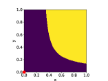
(a) MVI heatmap

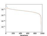
(b) Convergence of EG

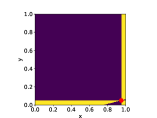
(c) MVI heatmap

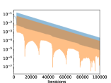
(d) Convergence of EG

Figure 1: Figures (a) and (b) display plots for one ratio game, and Figures (c) and (d) display plots for another; the games’ matrices are specified in Appendix C.1. Figures (a) and (c) plot the quantity ${\rm sign}(\langle F(z),z-z^{*}\rangle)$ for $z\in\Delta^{2}\times\Delta^{2}$, parameterized as $z:=(x,1-x,y,1-y)$; yellow denotes negative and purple denotes positive. The red dot denotes the equilibrium $z^{*}$. Figures (b) and (d) plot convergence of extragradient with learning rate 0.01, initialized at $z_{0}:=(1,0,1,0)$; note that $z_{0}$ is inside the region in which the MVI does not hold for each problem. The blue line plots the primal-dual gap $\max_{y^{\prime}}V(x^{(i)},y^{\prime})-\min_{x^{\prime}}V(x^{\prime},y^{(i)})$ and the orange line plots the primal gap $\max_{y^{\prime}}V(x^{(i)},y^{\prime})-V(x^{*},y^{*})$.

On the MVI condition.

For nonconvex-nonconcave minimax problems, the only general tool we are aware of for establishing last-iterate convergence for the extragradient method and its relatives is the Minty Variational Inequality (MVI) property (Facchinei and Pang, 2007; Lin et al., 2018; Mertikopoulos and Staudigl, 2018; Mertikopoulos et al., 2019; Gidel et al., 2019a). For $z=(x,y)$ and $F(z)\vcentcolon=(\nabla_{x}f(x,y),-\nabla_{y}f(x,y))$, the MVI property requires that there exists a point $z^{\star}\in\mathcal{Z}\vcentcolon=\mathcal{X}\times\mathcal{Y}$ such that

$$\left\langle F(z),z-z^{\star}\right\rangle\geq{}0\quad\forall{}z\in\mathcal{Z}.$$ (MVI)

For general minimax problems, the MVI property is typically applied with $z^{\star}$ as a Nash equilibrium (Mertikopoulos et al., 2019). We show that this condition fails in stochastic games, even for the simple ratio game in (12)

Proposition 2.

Fix $\epsilon,s\in(0,1)$ with $\epsilon<\frac{1-s}{2s}$. Suppose we take

$$R=\left(\begin{matrix}-1&\epsilon\\ -\epsilon&0\end{matrix}\right),\quad\text{and}\quad S=\left(\begin{matrix}s&s\\ 1&1\end{matrix}\right).$$ (12)

Then the ratio game defined by (12) has the following properties: (1) there is a unique Nash equilibrium $z^{*}=(z^{*},y^{*})$ given by $x^{*}=y^{*}=(0,1)$, (2) $\zeta\geq{}s$, (3) there exists $z=(x,y)\in\Delta(\mathcal{A})\times\Delta(\mathcal{B})$ so that $\langle F(z),z-z^{*}\rangle<0$.

Figure 1(a) plots the sign of $\left\langle F(z),z-z^{\star}\right\rangle$ for the game in (12) as a function of the players’ parameters, which changes based on whether they belong to one of two regions, and Figure 1(b) shows that extragradient readily converges to $z^{\star}$ in spite of the failure of MVI. While this example satisfies the MVI property locally around $z^{\star}$, Figure 1(c) shows a randomly generated game (Appendix C.1) for which the MVI property fails to hold even locally. Nonetheless, Figure 1(d) shows that extragradient converges for this example, albeit more slowly, and with oscillations. This leads to our open problem.

Open Problem 1.

Does the extragradient method with constant learning rate have last-iterate convergence for the ratio game (11) for any fixed $\zeta>0$?

Additional experiments with multi-state games generated at random suggest that the extragradient method has last-iterate convergence for general stochastic games with a positive stopping probability. Proving such a convergence result for extragradient or for relatives such as the optimistic gradient method would be of interest not only because it would guarantee last-iterate convergence, but because it would provide an algorithm that is strongly independent in the sense that two-timescale updates are not required.

5.2 Related Work

Issues of independence in MARL have enjoyed extensive investigation. We refer the reader to Zhang et al. (2019a) for a comprehensive overview and discuss some particularly relevant related work below.

Stochastic games.

Beginning with their introduction by Shapley (1953), there is a long line of work developing computationally efficient algorithms for multi-agent RL in stochastic games (Littman, 1994; Hu and Wellman, 2003; Bu et al., 2008). While centralized, coordinated MARL algorithms such as self-play have recently enjoyed some advances in terms of non-asymptotic guarantees Brafman and Tennenholtz (2002); Wei et al. (2017); Bai and Jin (2020); Xie et al. (2020); Zhang et al. (2020), independent RL has seen less development, with a few exceptions we discuss below.

A recent line of work (Srinivasan et al., 2018; Omidshafiei et al., 2019; Lockhart et al., 2019) shows that for zero-sum extensive form games (EFG), independent policy gradient methods can be formulated in the language of counterfactual regret minimization (Zinkevich et al., 2008), and uses this observation to derive convergence guarantees. Unfortunately, for the general zero-sum stochastic games we consider, reducing to an EFG results in exponential blowup in size with respect to horizon.

Arslan and Yüksel (2017) introduce an algorithm for learning stochastic games which can be viewed as a 2-timescale method and show convergence (though without rates) in a somewhat different setting from ours. Perolat et al. (2018) provide asymptotic guarantees for an independent two-timescale actor-critic method in zero-sum stochastic games with a “simultaneous-move multistage” structure in which each state can only be visited once. Our result is somewhat more general since it works for arbitrary infinite-horizon stochastic games, and is non-asymptotic.

Zhang et al. (2019b); Bu et al. (2019) recently gave global convergence results for policy gradient methods in two-player zero-sum linear-quadratic games. These results show that if the min-player follows policy gradient updates and the max-player follows the best response at each timestep, the min-player will converge to a Nash equilibrium. These results do not satisfy the independence property defined in Section 3, since they follow an inner-loop/outer-loop structure and assume exact access to gradients of the value function. Interestingly, Mazumdar et al. (2020) show that for general-sum linear-quadratic games, independent policy gradient methods can fail to converge even locally.

Two concurrent works also develop provable independent learning algorithms for stochastic games. Lee et al. (2020) show that the optimistic gradient algorithm obtains linear rates in the full-information and finite-horizon (undiscounted) setting, where the transition probability function $P$ is known and we have exact access to gradients. Their rate depends on the constant in a certain restricted secant inequality; this constant can be arbitrarily small even in the setting of matrix games (i.e., a single state, $\zeta=1$, and fixed $A,B$), which causes the rate to be arbitrarily slow. In a setting very similar to that of this paper, Bai et al. (2020) propose a model-free upper confidence bound-based algorithm, Nash V-learning, which satisfies the independent learning requirement and has near-optimal sample complexity, achieving superior dependence to Theorem 1 on the parameters $S,A,B,\zeta$, as well as no dependence on $C_{\mathcal{G}}$. However, their work has the limitation of only learning non-Markovian policies, whereas the policies learned by 2-timescale SGDA are Markovian (i.e., only depend on the current state).

Minimax optimization and (non-monotone) variational inequalities.

Since the objective $V_{\rho}(x,y)$ is continuous, a natural approach to minimizing it is to appeal to black-box algorithms for nonconvex-nonconcave minimization, and more broadly non-montone variational inequalities. In particular, the gradient dominance condition implies that all first-order stationary points are Nash equilibria. Unfortunately, compared to the single-player setting, where many algorithms such as gradient descent find first-order stationary points for arbitrary smooth, nonconvex functions, existing algorithms for non-monotone variational inequalities all require additional assumptions that are not satisfied in our setting. Mertikopoulos et al. (2019) give convergence guarantees for non-monotone variational inequalities satisfying the so-called MVI property, which we show fails even for single-state zero-sum stochastic games (Section 5.1). Yang et al. (2020) give an alternating gradient descent algorithm which succeeds for nonconvex-nonconcave games under a two-sided Polyak-Łojasiewicz condition, but this condition (which leads to linear convergence) is also not satisfied in our setting. Another complementary line of work develops algorithms for nonconvex-concave problems (Rafique et al., 2018; Thekumparampil et al., 2019; Lu et al., 2020; Nouiehed et al., 2019; Kong and Monteiro, 2019; Lin et al., 2020).

5.3 Future Directions

We presented the first independent policy gradient algorithms for competitive reinforcement learning in zero-sum stochastic games. We hope our results will serve as a starting point for developing a more complete theory for independent reinforcement learning in competitive RL and multi-agent reinforcement learning. Beyond Open Problem 1, there are a number of questions raised by our work.

Efroni et al. (2020) have recently shown how to improve the convergence rates for policy gradient algorithms in the single-agent setting by incorporating optimism. Finding a way to use similar techniques in the multi-agent setting under the independent learning requirement could be another promising direction for future work.

Many games of interest are not zero-sum, and may involve more than two players or be cooperative in nature. It would be useful to extend our results to these settings, albeit likely for weaker solution concepts, and to derive a tighter understanding of the optimization geometry for these settings.

On the technical side, there are a number of immediate technical extensions of our results which may be useful to pursue, including (1) extending to linear function approximation, (2) extending to other policy parameterizations such as soft-max, and (3) actor-critic and natural policy gradient-based variants (Agarwal et al., 2020).

Appendix A Proofs from Section 4

A.1 Additional Notation

Q-functions and advantage functions.

For policies $\pi_{1},\pi_{2}$, we let $Q^{\pi_{1},\pi_{2}}(s,a,b)$ denote the $Q$-value function:

$$Q^{\pi_{1},\pi_{2}}(s,a,b):=\mathbb{E}_{\pi_{1},\pi_{2}}\left[\sum_{t=0}^{T}R(s_{t},a_{t},b_{t})|s_{0}=s,a_{0}=a,b_{0}=b\right],$$

and we let $A^{\pi_{1},\pi_{2}}(s,a,b)=Q^{\pi_{1},\pi_{2}}(s,a,b)-V_{s}(\pi_{1},\pi_{2})$ denote the advantage function.

Throughout this section we abbreviate $V_{\rho}(x,y)=V_{\rho}(\pi_{x},\pi_{y})$, where $\pi_{x}$ and $\pi_{y}$ use the $\varepsilon$-greedy direct parameterization in Assumption 1.

A.2 Full Version of Theorem 1 and Proof

The full version of Theorem 1 is as follows.

Theorem 1a.

Let $\epsilon>0$ be given. Suppose both players follow the independent policy gradient scheme (3) with the parametrization in Assumption 1. If the learning rates satisfy $\eta_{x}=\Theta\left(\frac{\epsilon_{0}^{10.5}\zeta^{44.5}}{C_{\mathcal{G}}^{15.5}(A\vee B)^{9.75}S^{0.75}}\right)$ and $\eta_{y}=\Theta\left(\frac{\epsilon^{6}\zeta^{27}}{C_{\mathcal{G}}^{9}(A\vee B)^{6}\sqrt{S}}\right)$ and $\varepsilon_{x}=\Theta\left(\frac{\zeta^{3}\cdot\epsilon}{\sqrt{S}\sqrt{A\vee B}C_{\mathcal{G}}}\right)$ and $\varepsilon_{y}=\Theta\left(\frac{\zeta^{8}\epsilon^{2}}{C_{\mathcal{G}}^{3}(A\vee B)\sqrt{S}}\right)$, then we are guaranteed that

$$\textstyle\operatorname{\mathbb{E}}\left[\frac{1}{N}\sum_{i=1}^{N}\max_{\pi_{2}}V_{\rho}(\pi_{x^{{\scriptscriptstyle(i)}}},\pi_{2})\right]-\min_{\pi_{1}}\max_{\pi_{2}}V_{\rho}(\pi_{1},\pi_{2})\leq{}\epsilon$$ (13)

after $N=O\left(\frac{(A\vee B)^{10.75}S^{1.25}C_{\mathcal{G}}^{17.5}}{\epsilon^{12.5}\zeta^{48.5}}\right)$ episodes.

Proof of Theorem 1a.

This result is essentially an immediate consequence of Theorem 2a. As a first step, we observe that $D_{\mathcal{X}},D_{\mathcal{Y}}\leq{}\sqrt{S}$. Next, we observe that from Lemma 4, both players have $\ell\vcentcolon={}\frac{4A\vee{}B}{\zeta^{3}}$-jointly-Lipschitz gradients:

$$\left\|\nabla_{x}V_{\rho}(x,y)-\nabla_{x}V_{\rho}(x^{\prime},y^{\prime})\right\|_{2}\leq\frac{4(1-\zeta)A}{\zeta^{3}}\|(x,y)-(x^{\prime},y^{\prime})\|_{2},$$

$$\left\|\nabla_{y}V_{\rho}(x,y)-\nabla_{y}V_{\rho}(x^{\prime},y^{\prime})\right\|_{2}\leq\frac{4(1-\zeta)B}{\zeta^{3}}\|(x,y)-(x^{\prime},y^{\prime})\|_{2}.$$

Similarly, by Proposition 3, the function value $V_{\rho}(x,y)$ is $L\vcentcolon={}\frac{2\sqrt{A\vee{}B}}{\zeta^{2}}$-Lipschitz:

$$\left\|\nabla{}_{x}V_{\rho}(x,y)\right\|\leq{}\frac{\sqrt{A}}{\zeta^{2}},\quad\text{and}\quad\left\|\nabla{}_{y}V_{\rho}(x,y)\right\|\leq{}\frac{\sqrt{B}}{\zeta^{2}}.$$

Note that $L/\ell\leq 1$ since $A\wedge B\wedge 1/\zeta\geq 1$. Lemma 2 guarantees that both players have bounded variance:

$$\operatorname{\mathbb{E}}_{\pi_{x},\pi_{y}}\left\|\widehat{\nabla}_{x}-\nabla{}_{x}V_{\rho}(x,y)\right\|^{2}\leq{}24\frac{A^{2}}{\varepsilon_{x}\zeta^{4}},\quad\text{and}\quad\operatorname{\mathbb{E}}_{\pi_{x},\pi_{y}}\left\|\widehat{\nabla}_{y}-\nabla{}_{y}V_{\rho}(x,y)\right\|^{2}\leq{}24\frac{B^{2}}{\varepsilon_{y}\zeta^{4}}.$$ (14)

Lemma 1a guarantees that the gradient domination conditions 2 and 3 of Assumption 2 are satisfied with $\mu_{y}=\mu_{x}=\zeta/C_{\mathcal{G}}$, and additive components $\varepsilon_{x},\varepsilon_{y}$ equal to $\frac{2\varepsilon_{x}}{\zeta^{2}}$ and $\frac{2\varepsilon_{y}}{\zeta^{2}}$, respectively:

$$\frac{\zeta}{C_{\mathcal{G}}}\left(V_{\rho}(x,y)-\min_{x^{\prime}}V_{\rho}(x^{\prime},y)\right)-\frac{2\varepsilon_{x}}{\zeta^{2}} \leq{}\max_{\bar{x}\in\Delta(\mathcal{A})^{\left\lvert\mathcal{S}\right\rvert}}\left\langle\nabla_{x}V_{\rho}(x,y),x-\bar{x}\right\rangle,$$

and

$$\frac{\zeta}{C_{\mathcal{G}}}\left(\max_{y^{\prime}}V_{\rho}(x,y^{\prime})-V_{\rho}(x,y)\right)-\frac{2\varepsilon_{y}}{\zeta^{2}} \leq{}\max_{\bar{y}\in\Delta(\mathcal{B})^{\left\lvert\mathcal{S}\right\rvert}}\left\langle\nabla_{y}V_{\rho}(x,y),\bar{y}-y\right\rangle.$$

Note that $L/\ell<1$. By Theorem 2a, for a desired accuracy level $\epsilon>0$, if we set:

$$\eta_{y} =\Theta\left(\frac{\epsilon^{4}\zeta^{15}\varepsilon_{y}}{C_{\mathcal{G}}^{2}(A\vee B)^{5}}\right)=\Theta\left(\frac{\epsilon^{4}(\zeta/C_{\mathcal{G}})^{2}}{((A\vee B)/\zeta^{3})^{3}((A\vee B)/\zeta^{4}+B^{2}/(\varepsilon_{y}\zeta^{4}))}\right),$$ (15)

$$\eta_{x} =\Theta\left(\frac{\epsilon^{8}\zeta^{27}\varepsilon_{y}\sqrt{\varepsilon_{x}}}{C_{\mathcal{G}}^{4}(A\vee B)^{8.5}}\right)$$ (16)

$$=\Theta\left(\frac{\epsilon^{8}(\zeta/C_{\mathcal{G}})^{4}}{((A\vee B)/\zeta^{3})^{5}\frac{\sqrt{A\vee B}}{\zeta^{2}}\cdot((A\vee B)/\zeta^{4}+B^{2}/(\varepsilon_{y}\zeta^{4}))\sqrt{(A\vee B)/\zeta^{4}+A^{2}/(\varepsilon_{x}\zeta^{4})}}\right),$$

$$N \geq\Omega\left(\frac{\sqrt{S}\cdot\frac{A\vee B}{\zeta^{2}}}{\epsilon^{2}\eta_{x}}\right),$$ (17)

we have that

$$\frac{1}{N+1}\sum_{i=0}^{N}\max_{y}V_{\rho}(x^{(i)},y)-\min_{x}\max_{y}V_{\rho}(x,y) \leq O\left(\frac{\epsilon C_{\mathcal{G}}}{\zeta}+\frac{\varepsilon_{x}C_{\mathcal{G}}}{\zeta^{3}}+\frac{\sqrt{(A\vee B)/\zeta^{3}}\sqrt{\varepsilon_{y}/\zeta^{2}}(C_{\mathcal{G}}/\zeta)}{\sqrt{\zeta/C_{\mathcal{G}}}}\right)$$

$$\leq O\left(\frac{\epsilon C_{\mathcal{G}}}{\zeta}+\frac{\varepsilon_{x}C_{\mathcal{G}}}{\zeta^{3}}+\frac{\sqrt{\varepsilon_{y}}C_{\mathcal{G}}^{1.5}\sqrt{A\vee B}}{\zeta^{4}}\right).$$ (18)

Recall that $x\mapsto\pi_{x},y\mapsto\pi_{y}$ denote the $\varepsilon_{x}$- and $\varepsilon_{y}$-greedy parametrizations, respectively (where $\varepsilon_{x},\varepsilon_{y}$ are as in the statement of Theorem 1a). Then for any $\pi_{1}:\mathcal{S}\rightarrow\Delta(\mathcal{A})$ (respectively, $\pi_{2}:\mathcal{S}\rightarrow\Delta(\mathcal{B})$), there is some $x\in\Delta(\mathcal{A})^{S}$ (respectively, $y\in\Delta(\mathcal{B})^{s}$) so that $\|\pi_{1}-\pi_{x}\|\leq 2\sqrt{S}\varepsilon_{x}$ (respectively, $\|\pi_{2}-\pi_{y}\|\leq 2\sqrt{S}\varepsilon_{y}$) for each $s\in\mathcal{S},a\in\mathcal{A}$ (respectively, $b\in\mathcal{B}$). Moreover, recall that Proposition 3 shows that the function $(x,y)\mapsto V_{\rho}(x,y)$ is $L$-Lipschitz for any $\varepsilon$-greedy parametrization, in particular for the one given by $\varepsilon_{x}=\varepsilon_{y}=0$. Thus,

$$\left|\left(\frac{1}{N+1}\sum_{i=0}^{N}\max_{y}V_{\rho}(x^{(i)},y)-\min_{x}\max_{y}V_{\rho}(x,y)\right)-\left(\frac{1}{N+1}\sum_{i=0}^{N}\max_{\pi_{2}}V_{\rho}(\pi_{x^{(i)}},\pi_{2})-\min_{\pi_{1}}\max_{\pi_{2}}V_{\rho}(\pi_{1},\pi_{2})\right)\right|$$

$$\leq O\left(\frac{\sqrt{S}(\varepsilon_{x}\vee\varepsilon_{y})\sqrt{A\vee B}}{\zeta^{2}}\right).$$

From (18) it now follows that

$$\frac{1}{N+1}\sum_{i=0}^{N}\max_{\pi_{2}}V_{\rho}(\pi_{x^{(i)}},\pi_{2})-\min_{\pi_{1}}\max_{\pi_{2}}V_{\rho}(\pi_{1},\pi_{2})\leq O\left(\frac{\epsilon C_{\mathcal{G}}}{\zeta}+\frac{\varepsilon_{x}C_{\mathcal{G}}}{\zeta^{3}}+\frac{\sqrt{\varepsilon_{y}}C_{\mathcal{G}}^{1.5}\sqrt{A\vee B}}{\zeta^{4}}+\frac{\sqrt{S}(\varepsilon_{x}\vee\varepsilon_{y})\sqrt{A\vee B}}{\zeta^{2}}\right).$$

To achieve a desired accuracy level $\epsilon_{0}$, it follows from (15), (16), and (17) that if we set

$$\varepsilon_{x}=\Theta\left(\frac{\zeta^{3}\cdot\epsilon_{0}}{\sqrt{S}\sqrt{A\vee B}C_{\mathcal{G}}}\right),\qquad\varepsilon_{y}=\Theta\left(\frac{\zeta^{8}\epsilon_{0}^{2}}{C_{\mathcal{G}}^{3}(A\vee B)\sqrt{S}}\right),\qquad\epsilon\leq O\left(\frac{\zeta\epsilon_{0}}{C_{\mathcal{G}}}\right),$$

and

$$\eta_{y} =\Theta\left(\frac{\epsilon_{0}^{6}\zeta^{27}}{C_{\mathcal{G}}^{9}(A\vee B)^{6}\sqrt{S}}\right)=\Theta\left(\frac{\left(\zeta\epsilon_{0}/C_{\mathcal{G}}\right)^{4}\zeta^{15}\cdot\frac{\zeta^{8}\epsilon_{0}^{2}}{C_{\mathcal{G}}^{3}(A\vee B)\sqrt{S}}}{C_{\mathcal{G}}^{2}(A\vee B)^{5}}\right),$$

$$\eta_{x} =\Theta\left(\frac{\epsilon_{0}^{10.5}\zeta^{44.5}}{C_{\mathcal{G}}^{15.5}(A\vee B)^{9.75}S^{0.75}}\right)=\Theta\left(\frac{(\zeta\epsilon_{0}/C_{\mathcal{G}})^{8}\zeta^{27}\left(\frac{\zeta^{8}\epsilon_{0}^{2}}{C_{\mathcal{G}}^{3}(A\vee B)\sqrt{S}}\right)\sqrt{\frac{\zeta^{3}\cdot\epsilon_{0}}{\sqrt{S}\sqrt{A\vee B}C_{\mathcal{G}}}}}{C_{\mathcal{G}}^{4}(A\vee B)^{8.5}}\right),$$

$$N =\Omega\left(\frac{(A\vee B)^{10.75}S^{1.25}C_{\mathcal{G}}^{17.5}}{\epsilon_{0}^{12.5}\zeta^{48.5}}\right)\geq\Omega\left(\frac{\sqrt{S}\cdot\frac{A\vee B}{\zeta^{2}}}{(\zeta\epsilon_{0}/C_{\mathcal{G}})^{2}\eta_{x}}\right),$$

then we have

$$\frac{1}{N+1}\sum_{i=0}^{N}\max_{\pi_{2}}V_{\rho}(\pi_{x^{(i)}},\pi_{2})-\min_{\pi_{1}}\max_{\pi_{2}}V_{\rho}(\pi_{1},\pi_{2})\leq\epsilon_{0}.$$

∎

A.3 Proofs for Additional Results

Proof of Proposition 1.

We define the following game $\mathcal{G}$ with state space $\mathcal{S}:=\{1,2,3,4,5\}$, action spaces $\mathcal{A}=\mathcal{B}=\{0,1\}$, and any stopping probability $\zeta>0$.

The transitions and rewards are as follows:

• In state 1, with probability $\zeta$, the game stops. Conditioned on not stopping:

  • If actions $(0,0)$ are taken, the game moves to state 2.

  • If actions $(0,1)$ are taken, the game moves to state 3.

  • If actions $(1,0)$ are taken, the game moves to state 4.

  • If actions $(1,1)$ are taken, the game moves to state 5.

  Both players receive 0 reward in state 1.

• In state $2\leq i\leq 5$, the game stops with probability $\zeta$, and otherwise always moves back to state 1. Furthermore, player 1 receives reward $i-1$ and player 2 receives reward $1-i$ (regardles of their actions).

Let the initial state distribution $\rho=\delta_{1}$ be defined by

$$\rho(1)=\rho(2)=\rho(4)=\rho(5)=1/4,\quad\text{and}\quad\rho(3)=0.$$

Clearly, the value $V_{\rho}({\pi_{1},\pi_{2}})$ of the game depends only on the policies at state 1, i.e., $\pi_{1}(\cdot|1),\pi_{2}(\cdot|1)$. If $\pi_{1}(0|1)=\pi_{2}(1|1)=1$, then certainly $d^{\pi_{1},\pi_{2}}_{\rho}(3)>0$, and therefore $\max_{\pi_{1},\pi_{2}}\left\|\frac{d_{\rho}^{\pi_{1},\pi_{2}}}{\rho}\right\|_{\infty}$ is infinite.

On the other hand, let us now consider the best-response policies:

• For any policy $\pi_{1}$ of the min-player, all policies $\pi_{2}\in\Pi_{2}^{*}(\pi_{1})$ of the max-player satisfy $\pi_{2}(0|1)=1$. This follows since player 2 prefers state 2 to state 3, and state 4 to state 5.

  In particular, for any pair $(\pi_{1},\pi_{2})$ with $\pi_{2}\in\Pi_{2}^{*}(\pi_{1})$, we have that $d_{\rho}^{\pi_{1},\pi_{2}}(3)=0$.

• For any policy $\pi_{2}$ of the max-player, all policies $\pi_{1}\in\Pi_{1}^{*}(\pi_{1})$ of the min-player satisfy $\pi_{1}(1|0)=1$. This follows since player 1 prefers state 4 to state 2, and state 5 to state 3.

  In particular, for any pair $(\pi_{1},\pi_{2})$ with $\pi_{1}\in\Pi_{1}^{*}(\pi_{2})$, we have that $d_{\rho}^{\pi_{1},\pi_{2}}(3)=0$.

It follows that

$$C_{\mathcal{G}}=\max\left\{\max_{\pi_{2}}\min_{\pi_{1}\in\Pi^{\star}_{1}(\pi_{2})}\left\|\frac{d^{\pi_{1},\pi_{2}}_{\rho}}{\rho}\right\|_{\infty},\max_{\pi_{1}}\min_{\pi_{2}\in\Pi^{\star}_{2}(\pi_{1})}\left\|\frac{d^{\pi_{1},\pi_{2}}_{\rho}}{\rho}\right\|_{\infty}\right\}<\infty,$$

which completes the proof of the proposition. ∎

A.4 Supporting Lemmas

Lemma 2.

Suppose that players follow that $\varepsilon$-greedy direct parameterization in Assumption 1 with parameters $\varepsilon_{x}$ and $\varepsilon_{y}$. Given parameters $x\in\Delta(\mathcal{A})^{\left\lvert\mathcal{S}\right\rvert},y\in\Delta(\mathcal{A})^{\left\lvert\mathcal{S}\right\rvert}$ suppose the players estimate their gradients using the REINFORCE estimator:

$$\widehat{\nabla}_{x}\vcentcolon={}R_{T}\sum_{t=0}^{T}\nabla\log\pi_{x}(a_{t}\mid{}s_{t}),\quad\widehat{\nabla}_{y}\vcentcolon={}R_{T}\sum_{t=0}^{T}\nabla\log\pi_{y}(b_{t}\mid{}s_{t}),$$ (19)

under trajectories obtained by following $\pi_{x}$ and $\pi_{y}$. Then we have

$$\mathbb{E}_{\pi_{x},\pi_{y}}\widehat{\nabla}_{x}=\nabla_{x}V_{\rho}(\pi_{x},\pi_{y}),\qquad\mathbb{E}_{\pi_{x},\pi_{y}}\widehat{\nabla}_{y}=\nabla_{y}V_{\rho}(\pi_{x},\pi_{y}),$$ (20)

and

$$\operatorname{\mathbb{E}}_{\pi_{x},\pi_{y}}\left\|\widehat{\nabla}_{x}-\nabla{}_{x}V_{\rho}(x,y)\right\|^{2}\leq{}24\frac{A^{2}}{\varepsilon_{x}\zeta^{4}},\quad\text{and}\quad\operatorname{\mathbb{E}}_{\pi_{x},\pi_{y}}\left\|\widehat{\nabla}_{y}-\nabla{}_{y}V_{\rho}(x,y)\right\|^{2}\leq{}24\frac{B^{2}}{\varepsilon_{y}\zeta^{4}}.$$ (21)

Proof of Lemma 2.

We carry the calculation out for the $x$ player, as the $y$ player follows an identical argument. We start by proving that the gradient estimator is unbiased (i.e., (20)). Let $\mathcal{T}$ denote the (infinite) set of all possible trajectories, and for a trajectory $\tau=(s_{t},a_{t},b_{t},r_{t})_{0\leq t\leq T}$, in $\mathcal{T}$, let $R(\tau):=\sum_{t=0}^{T}r_{t}$ denote the total reward associated with $\tau$, and for policies $\pi_{1},\pi_{2}$, let

$$\operatorname{Pr}^{\pi_{1},\pi_{2}}(\tau):=\prod_{t=0}^{T}\pi_{1}(a_{t}|s_{t})\pi_{2}(b_{t}|s_{t})P(s_{t+1}|s_{t},a_{t},b_{t})$$

be the probability of realizing $\tau$. (Here, we let $s_{T+1}$ denote the event that the game stops at time $T$) Let $T(\tau)$ denote the last time step of trajectory $\tau$. Then

$$\nabla_{x}V_{\rho}(x,y)$$

$$=\nabla_{x}\sum_{\tau\in\mathcal{T}}R(\tau)\operatorname{Pr}^{\pi_{x},\pi_{y}}(\tau)$$

$$=\sum_{\tau\in\mathcal{T}}R(\tau)\nabla_{x}\operatorname{Pr}^{\pi_{x},\pi_{y}}(\tau)$$

$$=\sum_{\tau\in\mathcal{T}}R(\tau)\operatorname{Pr}^{\pi_{x},\pi_{y}}(\tau)\nabla_{x}\log\operatorname{Pr}^{\pi_{x},\pi_{y}}(\tau)$$

$$=\sum_{\tau\in\mathcal{T}}R(\tau)\operatorname{Pr}^{\pi_{x},\pi_{y}}(\tau)\nabla_{x}\left(\sum_{t=0}^{T(\tau)}\log\pi_{x}(a_{t}|s_{t})+\log\pi_{y}(b_{t}|s_{t})\right)$$

$$=\mathbb{E}_{\pi_{x},\pi_{y}}\left[\left(\sum_{t=0}^{T}r_{t}\right)\sum_{t=0}^{T}\nabla_{x}\log\pi_{x}(a_{t}|s_{t})\right]$$

$$=\mathbb{E}_{\pi_{x},\pi_{y}}\left[\widehat{\nabla}_{x}\right].$$

A similar calculation shows that $\mathbb{E}_{\pi_{x},\pi_{y}}\left[\widehat{\nabla}_{y}\right]=\nabla_{y}V_{\rho}(x,y)$.

We proceed to bound the variance of the gradient estimator (i.e., establish (21)). Since the gradient estimator is unbiased, we have

$$\operatorname{\mathbb{E}}_{\pi_{x},\pi_{y}}\left\|\widehat{\nabla}_{x}-\nabla{}_{x}V_{\rho}(x,y)\right\|^{2}\leq{}\operatorname{\mathbb{E}}_{\pi_{x},\pi_{y}}\left\|\widehat{\nabla}_{x}\right\|^{2}\leq{}\operatorname{\mathbb{E}}_{\pi_{x},\pi_{y}}\left\|R_{T}\sum_{t=0}^{T}\nabla\log\pi_{x}(a_{t}\mid{}s_{t})\right\|^{2}.$$

Next, we have

$$\operatorname{\mathbb{E}}_{\pi_{x},\pi_{y}}\left\|R_{T}\sum_{t=0}^{T}\nabla\log\pi_{x}(a_{t}\mid{}s_{t})\right\|^{2} \leq{}\operatorname{\mathbb{E}}_{\pi_{x},\pi_{y}}\left[(T+1)^{2}\left\|\sum_{t=0}^{T}\nabla\log\pi_{x}(a_{t}\mid{}s_{t})\right\|^{2}\right]$$

$$\leq{}\operatorname{\mathbb{E}}_{\pi_{x},\pi_{y}}\left[(T+1)^{3}\sum_{t=0}^{T}\left\|\nabla\log\pi_{x}(a_{t}\mid{}s_{t})\right\|^{2}\right]$$

$$=\operatorname{\mathbb{E}}_{\pi_{x},\pi_{y}}\left[(T+1)^{3}\sum_{t=0}^{T}\sum_{s,a}(1-\varepsilon_{x})^{2}\mathbbm{1}\left\{s=s_{t},a=a_{t}\right\}\frac{1}{\pi_{x}^{2}(a\mid{}s)}\right],$$

$$\leq{}\operatorname{\mathbb{E}}_{\pi_{x},\pi_{y}}\left[(T+1)^{3}\sum_{t=0}^{T}\sum_{s,a}\mathbbm{1}\left\{s=s_{t},a=a_{t}\right\}\frac{1}{\pi_{x}^{2}(a\mid{}s)}\right],$$

where the equality is a consequence of the direct parameterization. We further simplify as

$$\operatorname{\mathbb{E}}_{\pi_{x},\pi_{y}}\left[(T+1)^{3}\sum_{t=0}^{T}\sum_{s,a}\mathbbm{1}\left\{s=s_{t},a=a_{t}\right\}\frac{1}{\pi_{x}^{2}(a\mid{}s)}\right] =\sum_{t=0}^{\infty}\sum_{s,a}\operatorname{\mathbb{E}}_{\pi_{x},\pi_{y}}\left[\mathbbm{1}_{t\leq{}T}\mathbbm{1}\left\{s=s_{t},a=a_{t}\right\}\frac{1}{\pi_{x}^{2}(a\mid{}s)}(T+1)^{3}\right]$$

$$=\sum_{t=0}^{\infty}\sum_{s,a}\operatorname{\mathbb{E}}_{\pi_{x},\pi_{y}}\left[\mathbbm{1}_{t\leq{}T}\mathbbm{1}\left\{s=s_{t},a=a_{t}\right\}\frac{1}{\pi_{x}^{2}(a\mid{}s)}(T+1)^{3}\right]$$

$$=\sum_{t=0}^{\infty}\sum_{s,a}\operatorname{\mathbb{E}}_{\pi_{x},\pi_{y}}\left[\mathbbm{1}_{t\leq{}T}\mathbbm{1}\{s_{t}=s\}\frac{1}{\pi_{x}(a\mid{}s)}(T+1)^{3}\right]$$

$$\leq{}\frac{A}{\varepsilon_{x}}\sum_{t=0}^{\infty}\sum_{s,a}\operatorname{\mathbb{E}}_{\pi_{x},\pi_{y}}\left[\mathbbm{1}_{t\leq{}T}\mathbbm{1}\{s_{t}=s\}(T+1)^{3}\right]$$

$$\leq\frac{A^{2}}{\varepsilon_{x}}\operatorname{\mathbb{E}}_{\pi_{x},\pi_{y}}\left[(T+1)^{4}\right].$$

To conclude, we observe that

$$\operatorname{\mathbb{E}}_{\pi_{x},\pi_{y}}\left[(T+1)^{4}\right]\leq{}\sum_{t=0}^{\infty}(1-\zeta)^{t}\zeta{}(t+1)^{4}\\ =\frac{\zeta}{1-\zeta}\sum_{t=1}^{\infty}(1-\zeta)^{t}t^{4}\\ \leq{}\frac{24}{\zeta^{4}}.$$

∎

Define, for any $s_{0}\in\mathcal{S}$ and policies $\pi_{1},\pi_{2}$,

$$\tilde{d}_{s_{0}}^{\pi_{1},\pi_{2}}(s):=\sum_{t\geq 0}\operatorname{Pr}^{\pi_{1},\pi_{2}}(s_{t}=s|s_{0}),$$

and $\tilde{d}_{\rho}^{\pi_{1},\pi_{2}}(s):=\mathbb{E}_{s_{0}\sim\rho}[\tilde{d}_{s_{0}}^{\pi_{1},\pi_{2}}(s)]$ be the un-normalized state visitation distribution. Also let $\operatorname{Pr}^{\pi_{1},\pi_{2}}(\tau|s_{0})$ (respectively, $\operatorname{Pr}^{\pi_{1},\pi_{2}}(\tau|\rho)$) be the distribution of trajectories $\tau$ given policies $\pi_{1},\pi_{1}$ and initial state $s_{0}$ (respectively, initial state distribution $\rho$).

Proposition 3.

In the direct parameterization with $\varepsilon$-greedy exploration (Assumption 1), we have, for all $s\in\mathcal{S},a\in\mathcal{A},b\in\mathcal{B}$,

$$\frac{\partial V_{\rho}(x,y)}{\partial x_{s,a}} =(1-\varepsilon_{x})\tilde{d}_{\rho}^{\pi_{x},\pi_{y}}(s)\mathbb{E}_{b\sim\pi_{y}(\cdot|s)}\left[Q^{\pi_{x},\pi_{y}}(s,a,b)\right]$$

$$\frac{\partial V_{\rho}(x,y)}{\partial y_{s,b}} =(1-\varepsilon_{y})\tilde{d}_{\rho}^{\pi_{x},\pi_{y}}(s)\mathbb{E}_{a\sim\pi_{x}(\cdot|s)}[Q^{\pi_{x},\pi_{y}}(s,a,b)].$$

and so it follows that for all $\varepsilon_{x},\varepsilon_{y}\geq 0$,

$$\left|\frac{\partial V_{\rho}}{\partial x_{s,a}}(x,y)\right| \leq\frac{1}{\zeta}d_{\rho}^{\pi_{x},\pi_{y}}(s)\left|\mathbb{E}_{b\sim y(\cdot|s)}[Q^{\pi_{x},\pi_{y}}(s,a,b)]\right|$$

$$\left|\frac{\partial V_{\rho}}{\partial y_{s,b}}(x,y)\right| \leq\frac{1}{\zeta}d_{\rho}^{\pi_{x},\pi_{y}}(s)\left|\mathbb{E}_{a\sim x(\cdot|s)}[Q^{\pi_{x},\pi_{y}}(s,a,b)]\right|.$$

As a consequence, $\left\|\nabla{}_{x}V_{\rho}(x,y)\right\|\leq{}\frac{\sqrt{A}}{\zeta^{2}}$ and $\left\|\nabla{}_{y}V_{\rho}(x,y)\right\|\leq{}\frac{\sqrt{B}}{\zeta^{2}}$.

Proof of Proposition 3.

Note that for any $s\in\mathcal{S}$, $\tilde{d}_{\rho}^{\pi_{1},\pi_{2}}(s)\leq\frac{d_{\rho}^{\pi_{1},\pi_{2}}(s)}{\zeta}$.

Fix any initial state $s_{0}\in\mathcal{S}$. Note that

$$\nabla_{x}V_{s_{0}}(x,y)$$

$$=\nabla_{x}\sum_{a_{0}\in\mathcal{A}}\pi_{x}(a_{0}|s_{0})\mathbb{E}_{b_{0}\sim\pi_{y}(\cdot|s_{0})}[Q^{\pi_{x},\pi_{y}}(s_{0},a_{0},b_{0})]$$

$$=\sum_{a_{0}}(\nabla_{x}\pi_{x}(a_{0}|s_{0}))\mathbb{E}_{b_{0}\sim\pi_{y}(\cdot|s_{0})}[Q^{\pi_{x},\pi_{y}}(s_{0},a_{0},b_{0})]+\sum_{a_{0}}\pi_{x}(a_{0}|s_{0})\mathbb{E}_{b_{0}\sim\pi_{y}(\cdot|s_{0})}[\nabla_{x}Q^{\pi_{x},\pi_{y}}(s_{0},a_{0},b_{0})]$$

$$=\sum_{a_{0}}\pi_{x}(a_{0}|s_{0})(\nabla_{x}\log\pi_{x}(a_{0}|s_{0}))\mathbb{E}_{b_{0}\sim\pi_{y}(\cdot|s_{0})}[Q^{\pi_{x},\pi_{y}}(s_{0},a_{0},b_{0})]$$

$$~{}~{}~{}~{}+\sum_{a_{0}}\pi_{x}(a_{0}|s_{0})\mathbb{E}_{b_{0}\sim\pi_{y}(\cdot|s_{0})}\left[\sum_{s_{1}}P(s_{1}|s_{0},a_{0},b_{0})\nabla_{x}V_{s_{1}}(x,y)\right]$$

$$=\mathbb{E}_{\tau\sim\operatorname{Pr}^{\pi_{x},\pi_{y}}(\cdot|s_{0})}\left[(\nabla_{x}\log\pi_{x}(a_{0}|s_{0}))Q^{\pi_{x},\pi_{y}}(s_{0},a_{0},b_{0})\right]$$

$$~{}~{}~{}~{}+\mathbb{E}_{\tau\sim\operatorname{Pr}^{\pi_{x},\pi_{y}}(\cdot|s_{0})}\left[\mathbbm{1}_{T\geq 1}\nabla_{x}V_{s_{1}}(x,y)\right].$$

Note that the above calculation holds also when $s_{0}$ is replaced with any distribution $\rho\in\Delta(\mathcal{S})$. It follows by induction and the fact that $\operatorname{Pr}[T\geq t]\leq(1-\zeta)^{t}$ for any $t\geq 0$ that for any $\rho\in\Delta(\mathcal{S})$,

$$\nabla_{x}V_{\rho}(x,y) =\mathbb{E}_{\tau\sim\operatorname{Pr}^{\pi_{x},\pi_{y}}(\cdot|s_{0})}\left[\sum_{t=0}^{T}(\nabla_{x}\log\pi_{x}(a_{t}|s_{t}))Q^{\pi_{x},\pi_{y}}(s_{t},a_{t},b_{t})\right]$$

$$=\sum_{s\in\mathcal{S}}\mathbb{E}_{a\sim\pi_{x}(\cdot|s)}\mathbb{E}_{b\sim\pi_{y}(\cdot|s)}\left[\tilde{d}_{\rho}^{\pi_{x},\pi_{y}}(s)(\nabla_{x}\log\pi_{x}(a|s))Q^{\pi_{x},\pi_{y}}(s,a,b)\right].$$

Thus, for any $s\in\mathcal{S},a\in\mathcal{A}$, we have

$$\frac{\partial V_{\rho}(x,y)}{\partial x_{s,a}}=(1-\varepsilon_{x})\tilde{d}_{\rho}^{\pi_{x},\pi_{y}}(s)\mathbb{E}_{b\sim\pi_{y}(\cdot|s)}\left[Q^{\pi_{x},\pi_{y}}(s,a,b)\right],$$

and so it follows that

$$\left|\frac{\partial V_{\rho}(x,y)}{\partial x_{s,a}}\right|\leq\frac{d_{\rho}^{\pi_{x},\pi_{y}}(s)}{\zeta}\left|\mathbb{E}_{b\sim\pi_{y}(\cdot|s)}\left[Q^{\pi_{x},\pi_{y}}(s,a,b)\right]\right|.$$

The inequality for the derivative with respect to $y$ follows in a symmetric manner. ∎

Lemma 3 (Performance difference lemma).

For all policies $\pi_{1},\pi_{1}^{\prime},\pi_{2},\pi_{2}^{\prime}$ and distributions $\rho\in\Delta(\mathcal{S})$,

$$V_{\rho}(\pi_{1},\pi_{2})-V_{\rho}(\pi_{1}^{\prime},\pi_{2}) =\sum_{s\in\mathcal{S}}\tilde{d}_{\rho}^{\pi_{1},\pi_{2}}(s)\mathbb{E}_{a\sim\pi_{1}(\cdot|s)}\mathbb{E}_{b\sim\pi_{2}(\cdot|s)}\left[A^{\pi_{1}^{\prime},\pi_{2}}(s,a,b)\right]$$

$$V_{\rho}(\pi_{1},\pi_{2})-V_{\rho}(\pi_{1},\pi_{2}^{\prime}) =\sum_{s\in\mathcal{S}}\tilde{d}_{\rho}^{\pi_{1},\pi_{2}}(s)\mathbb{E}_{a\sim\pi_{1}(\cdot|s)}\mathbb{E}_{b\sim\pi_{2}(\cdot|s)}\left[A^{\pi_{1}^{\prime},\pi_{2}}(s,a,b)\right].$$

Proof of Lemma 3.

Note that, for any $s\in\mathcal{S}$,

$$V_{s}(\pi_{1},\pi_{2})-V_{s}(\pi_{1}^{\prime},\pi_{2})$$

$$=\mathbb{E}_{\tau\sim\operatorname{Pr}^{\pi_{1},\pi_{2}}(\cdot|{s})}\left[\sum_{t=0}^{T}R(s_{t},a_{t},b_{t})\right]-V_{s}(\pi_{1}^{\prime},\pi_{2})$$

$$=\mathbb{E}_{\tau\sim\operatorname{Pr}^{\pi_{1},\pi_{2}}(\cdot|{s})}\left[\sum_{t=0}^{T}R(s_{t},a_{t},b_{t})+V_{s_{t}}(\pi_{1}^{\prime},\pi_{2})-V_{s_{t}}(\pi_{1}^{\prime},\pi_{2})\right]-V_{s}(\pi_{1}^{\prime},\pi_{2})$$

$$=\mathbb{E}_{\tau\sim\operatorname{Pr}^{\pi_{1},\pi_{2}}(\cdot|{s})}\left[\sum_{t=0}^{T}R(s_{t},a_{t},b_{t})+\mathbbm{1}_{t+1\leq T}V_{s_{t+1}}(\pi_{1}^{\prime},\pi_{2})-V_{s_{t}}(\pi_{1}^{\prime},\pi_{2})\right]$$

$$=\mathbb{E}_{\tau\sim\operatorname{Pr}^{\pi_{1},\pi_{2}}(\cdot|{s})}\left[\sum_{t=0}^{T}R(s_{t},a_{t},b_{t})+\mathbb{E}\left[\mathbbm{1}_{t+1\leq T}V_{s_{t+1}}(\pi_{1}^{\prime},\pi_{2})|s_{t},a_{t},b_{t}\right]-V_{s_{t}}(\pi_{1}^{\prime},\pi_{2})\right]$$

$$=\mathbb{E}_{\tau\sim\operatorname{Pr}^{\pi_{1},\pi_{2}}(\cdot|{s})}\left[\sum_{t=0}^{T}A^{\pi_{1}^{\prime},\pi_{2}}(s_{t},a_{t},b_{t})\right]$$

$$=\sum_{s^{\prime}\in\mathcal{S}}\tilde{d}_{s}^{\pi_{1},\pi_{2}}(s^{\prime})\mathbb{E}_{a\sim\pi_{1}(\cdot|s^{\prime})}\mathbb{E}_{b\sim\pi_{2}(\cdot|s^{\prime})}\left[A^{\pi_{1}^{\prime},\pi_{2}}(s^{\prime},a,b)\right].$$

The proof of the second inequality in the lemma is symmetric. ∎

Lemma 1a.

Suppose that players follow the $\varepsilon$-greedy direct parameterization of Assumption 1 with parameters $\varepsilon_{x}$ and $\varepsilon_{y}$. Then for all $x\in\Delta(\mathcal{A})^{\left\lvert\mathcal{S}\right\rvert}$, $y\in\Delta(\mathcal{B})^{\left\lvert\mathcal{S}\right\rvert}$ we have

$$V_{\rho}(x,y)-\min_{x^{\prime}}V_{\rho}(x^{\prime},y) \leq{}\min_{\pi_{1}\in\Pi_{1}^{*}(\pi_{y})}\left\|\frac{d_{\rho}^{\pi_{1},\pi_{y}}}{\rho}\right\|_{\infty}\left(\frac{1}{\zeta}\max_{\bar{x}\in\Delta(\mathcal{A})^{\left\lvert\mathcal{S}\right\rvert}}\left\langle\nabla_{x}V_{\rho}(x,y),x-\bar{x}\right\rangle+\frac{2\varepsilon_{x}}{\zeta^{3}}\right),$$ (22)

and

$$\max_{y^{\prime}}V_{\rho}(x,y^{\prime})-V_{\rho}(x,y) \leq{}\min_{\pi_{2}\in\Pi_{2}^{*}(\pi_{x})}\left\|\frac{d_{\rho}^{\pi_{x},\pi_{2}}}{\rho}\right\|_{\infty}\left(\frac{1}{\zeta}\max_{\bar{y}\in\Delta(\mathcal{B})^{\left\lvert\mathcal{S}\right\rvert}}\left\langle\nabla_{y}V_{\rho}(x,y),\bar{y}-y\right\rangle+\frac{2\varepsilon_{y}}{\zeta^{3}}\right),$$ (23)

Proof of Lemma 1.

We prove the inequality for $x$ player. The inequality for the $y$ player follows by symmetry. For a policy $\pi_{y}$, let $\pi_{1}^{*}(\pi_{y})\in\Pi_{1}^{*}(\pi_{y})$ denote a policy minimizing $\left\|\frac{d_{\rho}^{\pi_{1},\pi_{y}}}{\rho}\right\|_{\infty}$ (whose existence follows from compactness of the space of policies).

Using the performance difference lemma, we have

$$V_{\rho}(x,y)-\min_{x^{\prime}}V_{\rho}(x^{\prime},y)$$

$$\leq{}V_{\rho}(\pi_{x},\pi_{y})-V_{\rho}(\pi_{1}^{*}(\pi_{y}),\pi_{y})$$

$$=\sum_{s,a}\tilde{d}_{\rho}^{\pi^{\star}_{1}(\pi_{y}),\pi_{y}}(s)\pi^{\star}_{1}(\pi_{y})(a\mid{}s)\operatorname{\mathbb{E}}_{b\sim{}\pi_{y}(\cdot\mid{}s)}\left[-A^{\pi_{x},\pi_{y}}(s,a,b)\right]$$

$$\leq{}\sum_{s}\tilde{d}_{\rho}^{\pi^{\star}_{1}(\pi_{y}),\pi_{y}}(s)\max_{a}\operatorname{\mathbb{E}}_{b\sim{}\pi_{y}(\cdot\mid{}s)}\left[-A^{\pi_{x},\pi_{y}}(s,a,b)\right]$$

$$\leq{}\left\|\frac{\tilde{d}_{\rho}^{\pi^{\star}_{1}(\pi_{y}),\pi_{y}}}{\tilde{d}_{\rho}^{\pi_{x},\pi_{y}}(s)}\right\|_{\infty}\sum_{s}\tilde{d}_{\rho}^{\pi_{x},\pi_{y}}(s)\max_{a}\operatorname{\mathbb{E}}_{b\sim{}\pi_{y}(\cdot\mid{}s)}\left[-A^{\pi_{x},\pi_{y}}(s,a,b)\right].$$

We observe that $\left\|\frac{\tilde{d}_{\rho}^{\pi^{\star}_{1}(\pi_{y}),\pi_{y}}}{\tilde{d}_{\rho}^{\pi_{x},\pi_{y}}}\right\|_{\infty}\leq{}\frac{1}{\zeta}\left\|\frac{d_{\rho}^{\pi^{\star}_{1}(\pi_{y}),\pi_{y}}}{\rho}\right\|_{\infty}\leq{}\frac{1}{\zeta}C_{\mathcal{G}}$. Next, we have

$$\sum_{s,a}\tilde{d}_{\rho}^{\pi_{x},\pi_{y}}(s)\max_{a}\operatorname{\mathbb{E}}_{b\sim{}\pi_{y}(\cdot\mid{}s)}\left[-A^{\pi_{x},\pi_{y}}(s,a,b)\right]$$

$$=\max_{\bar{x}\in\Delta(\mathcal{A})^{\left\lvert\mathcal{S}\right\rvert}}\sum_{s,a}\tilde{d}_{\rho}^{\pi_{x},\pi_{y}}(s)\bar{x}_{s,a}\operatorname{\mathbb{E}}_{b\sim{}\pi_{y}(\cdot\mid{}s)}\left[-A^{\pi_{x},\pi_{y}}(s,a,b)\right]$$

$$=\max_{\bar{x}\in\Delta(\mathcal{A})^{\left\lvert\mathcal{S}\right\rvert}}\sum_{s,a}\tilde{d}_{\rho}^{\pi_{x},\pi_{y}}(s)(\pi_{x}(a\mid{}s)-\bar{x}_{s,a})\operatorname{\mathbb{E}}_{b\sim{}\pi_{y}(\cdot\mid{}s)}\left[Q^{\pi_{x},\pi_{y}}(s,a,b)\right]$$

$$=\max_{\bar{x}\in\Delta(\mathcal{A})^{\left\lvert\mathcal{S}\right\rvert}}\sum_{s,a}\tilde{d}_{\rho}^{\pi_{x},\pi_{y}}(s)((1-\varepsilon_{x})x_{s,a}+\varepsilon_{x}A^{-1}-\bar{x}_{s,a})\operatorname{\mathbb{E}}_{b\sim{}\pi_{y}(\cdot\mid{}s)}\left[Q^{\pi_{x},\pi_{y}}(s,a,b)\right],$$

$$\leq{}\max_{\bar{x}\in\Delta(\mathcal{A})^{\left\lvert\mathcal{S}\right\rvert}}\sum_{s,a}\tilde{d}_{\rho}^{\pi_{x},\pi_{y}}(s)((1-\varepsilon_{x})x_{s,a}+\varepsilon_{x}A^{-1}-\varepsilon_{x}\bar{x}_{s,a}-(1-\varepsilon_{x})\bar{x}_{s,a})\operatorname{\mathbb{E}}_{b\sim{}\pi_{y}(\cdot\mid{}s)}\left[Q^{\pi_{x},\pi_{y}}(s,a,b)\right]$$

$$\leq{}(1-\varepsilon_{x})\max_{\bar{x}\in\Delta(\mathcal{A})^{\left\lvert\mathcal{S}\right\rvert}}\sum_{s,a}\tilde{d}_{\rho}^{\pi_{x},\pi_{y}}(s)(x_{s,a}-\bar{x}_{s,a})\operatorname{\mathbb{E}}_{b\sim{}\pi_{y}(\cdot\mid{}s)}\left[Q^{\pi_{x},\pi_{y}}(s,a,b)\right]+\frac{2\varepsilon_{x}}{\zeta^{2}}$$

$$=\max_{\bar{x}\in\Delta(\mathcal{A})^{\left\lvert\mathcal{S}\right\rvert}}\left\langle\nabla_{x}V_{\rho}(x,y),x-\bar{x}\right\rangle+\frac{2\varepsilon_{x}}{\zeta^{2}},$$ (24)

where (24) follows from Proposition 3. Rearranging, this establishes that

$$V_{\rho}(x,y)-V_{\rho}(x^{\star}(y),y) \leq{}\left\|\frac{d_{\rho}^{\pi^{\star}_{1}(\pi_{y}),\pi_{y}}}{\rho}\right\|_{\infty}\left(\frac{1}{\zeta}\max_{\bar{x}\in\Delta(\mathcal{A})^{\left\lvert\mathcal{S}\right\rvert}}\left\langle\nabla_{x}V_{\rho}(x,y),x-\bar{x}\right\rangle+\frac{2\varepsilon_{x}}{\zeta^{3}}\right).$$

∎

The following lemma, which is a consequence of Lemma E.3 of Agarwal et al. (2020), establishes that the direct parameterization leads to Lipschitz gradients.

Lemma 4 (Smoothness).

For all starting states $s_{0}$, and for all policies $x,x^{\prime},y,y^{\prime}$, it holds that

$$\left\|\nabla_{x}V_{s_{0}}(x,y)-\nabla_{x}V_{s_{0}}(x^{\prime},y^{\prime})\right\|_{2}\leq\frac{4(1-\zeta)A}{\zeta^{3}}\|(x,y)-(x^{\prime},y^{\prime})\|_{2},$$

$$\left\|\nabla_{y}V_{s_{0}}(x,y)-\nabla_{y}V_{s_{0}}(x^{\prime},y^{\prime})\right\|_{2}\leq\frac{4(1-\zeta)A}{\zeta^{3}}\|(x,y)-(x^{\prime},y^{\prime})\|_{2}.$$

Appendix B Two-Timescale SGDA

B.1 Algorithm and Main Theorem

Throughout this section we will consider compact and convex subsets $\mathcal{X}\subset\mathbb{R}^{d_{x}},\mathcal{Y}\subset\mathbb{R}^{d_{y}}$ of Euclidean space. Our goal will be to find approximate equilibria for the game

$$\min_{x\in\mathcal{X}}\max_{y\in\mathcal{Y}}f(x,y),$$

where $f:\mathcal{X}\times\mathcal{Y}\rightarrow\mathbb{R}$ is a continuously differentiable function. We assume that we can only access $f$ through a stochastic first-order oracle (Assumption 3), and we analyze a two-timescale version of simultaneous gradient descent-ascent (SGDA) in this model. Before stating the algorithm, we state our regularity assumptions on the function $f$ and the oracle.

Define the max function $\Phi:\mathcal{X}\rightarrow\mathbb{R}$ and the min function $\Psi:\mathcal{Y}\rightarrow\mathbb{R}$ as follows:

$$\Phi(x):=\max_{y\in\mathcal{X}}f(x,y),\qquad\Psi(y):=\min_{x\in\mathcal{X}}f(x,y).$$

Moreover, let $D_{\mathcal{X}}$ denote the diameter of $\mathcal{X}$ and $D_{\mathcal{Y}}$ denote the diameter of $\mathcal{Y}$. We make the following assumptions about $f(x,y)$. To state the assumption, let $y^{\star}(x)\in\operatorname*{arg\,max}_{y\in\mathcal{Y}}f(x,y)$ and $x^{\star}(y)\in\operatorname*{arg\,min}_{x\in\mathcal{X}}f(x,y)$ denote arbitrary best-response functions for the $y$ and $x$ players, respectively.

Assumption 2.

Assume that $\mathcal{X}\subset\mathbb{R}^{d_{x}},\mathcal{Y}\subset\mathbb{R}^{d_{y}}$ are closed and compact subsets of Euclidean space and $f:\mathcal{X}\times\mathcal{Y}\rightarrow\mathbb{R}$. We assume that $f$ satisfies:

1. $f$ is $\ell$-smooth and $L$-Lipschitz.

2. For some constants $\varepsilon_{y}\geq 0,\mu_{y}>0$, for each $x\in\mathcal{X}$, the function $y\mapsto f(x,y)$ satisfies the following gradient domination condition:

   $$\max_{\bar{y}\in\mathcal{Y}:\left\|\bar{y}-y\right\|\leq{}1}\langle\bar{y}-y,\nabla_{y}f(x,y)\rangle\geq\mu_{y}\cdot(f(x,y^{*}(x))-f(x,y))-\varepsilon_{y}.$$

3. For some constants $\varepsilon_{x}\geq 0,\mu_{x}>0$, for each $y\in\mathcal{X}$, the function $x\mapsto f(x,y)$ satisfies the following gradient domination condition:

   $$\max_{\bar{x}\in\mathcal{X},\|\bar{x}-x\|\leq 1}\langle x-\bar{x},\nabla_{x}f(x,y)\rangle\geq\mu_{x}\cdot(f(x,y)-f(x^{*}(y),y))-\varepsilon_{x}.$$

Remark 1 (Empty interior).

If the interior of $\mathcal{X}\times\mathcal{Y}\subset\mathbb{R}^{d_{x}+d_{y}}$, denoted by $(\mathcal{X}\times\mathcal{Y})^{\circ}$, is empty (which is the case for the direct parametrization of policies in Markov games), then in order to ensure that $\nabla f(x,y)$ is well-defined on $\mathcal{X}\times\mathcal{Y}$, we make the technical assumption that $f$ is continuously differentiable on a closed neighborhood $\tilde{\mathcal{X}}\times\tilde{\mathcal{Y}}$, where $\mathcal{X}\subset\subset\tilde{\mathcal{X}},\mathcal{Y}\subset\subset\tilde{\mathcal{Y}}$, which may be assumed without loss of generality to be convex. It is straightforward to check that this assumption holds in our application to Markov games.

Suppose $f$ satisfies Assumption 2. In the event that the interior $(\mathcal{X}\times\mathcal{Y})^{\circ}$ is empty, by compactness of $\mathcal{X}$ and $\mathcal{Y}$, for any $\delta>0$, there are closed convex neighborhoods $\mathcal{X}_{\delta},\mathcal{Y}_{\delta}$ with $\mathcal{X}\subset\subset\mathcal{X}_{\delta},\mathcal{Y}\subset\subset\mathcal{Y}_{\delta}$, so that any point in $\mathcal{X}_{\delta}\times\mathcal{Y}_{\delta}$ is at most distance $\delta$ from a point in $\mathcal{X}\times\mathcal{Y}$, $f$ is $(\ell+\delta)$-smooth and $(L+\delta)$-Lipschitz on $\mathcal{X}_{\delta}\times\mathcal{Y}_{\delta}$, and items 2 and 3 hold for any $x\in\mathcal{X}_{\delta},y\in\mathcal{Y}_{\delta}$ with constants $\varepsilon_{y}+\delta$, $\mu_{y}-\delta$, $\mu_{x}-\delta$, and $\varepsilon_{x}+\delta$. We will use this fact in the proof of Lemma 12.

We formalize the stochastic first-order oracle model our algorithm works in as follows. In this section only, we will denote the iterates of stochastic gradient descent-ascent using $x_{t},y_{t}$ (as opposed to previous sections where we wrote $x^{(i)},y^{(i)}$).

Given a random variable $\xi\in\Xi$ with law $\mathbb{P}$ (for some sample space $\Xi$), a stochastic first-order oracle $G:\mathcal{X}\times\mathcal{Y}\times\Xi\rightarrow\mathbb{R}^{d_{x}+d_{y}}$ satisfies the following properties.

Assumption 3 (Stochastic first-order oracle).

For variance parameters $\sigma_{x},\sigma_{y}>0$, the stochastic oracle $G(x,y,\xi)=(G_{x}(x,y,\xi),G_{y}(x,y,\xi))$ satisfies:

$$\mathbb{E}[G(x,y,\xi)]=\nabla f(x,y),$$

$$\mathbb{E}[\|G_{x}(x,y,\xi)-\nabla_{x}f(x,y,\xi)\|^{2}]\leq\sigma_{x}^{2},$$

$$\mathbb{E}[\|G_{y}(x,y,\xi)-\nabla_{y}f(x,y,\xi)\|^{2}]\leq\sigma_{y}^{2}.$$

Given the stochastic first-order oracle $G=(G_{x},G_{y})$, the two-timescale stochastic simultaneous GDA algorithm (or SGDA) draws a sample $\xi_{t-1}\sim\mathbb{P}$, and performs the updates

$$x_{t} \leftarrow\mathcal{P}_{\mathcal{X}}\left(x_{t-1}-\eta_{x}G_{x}(x_{t-1},y_{t-1},\xi_{t-1})\right),$$ (25)

$$y_{t} \leftarrow\mathcal{P}_{\mathcal{Y}}\left(y_{t-1}+\eta_{y}G_{y}(x_{t-1},y_{t-1},\xi_{t-1}\right).$$ (26)

Main theorem.

Our main theorem for SGDA, Theorem 2a (the full version of Theorem 2), shows that if the learning rate $\eta_{x}$ of two-timescale SGDA is chosen sufficiently small relative to $\eta_{y}$, the iterates $x_{t}$ will approach, on average, the optimal point $x^{*}$.

For simplicity of presentation, we make the following assumptions regarding the various parameters: $\min\{L,\ell,\sigma_{x},\sigma_{y},1/\mu_{x},1/\mu_{y}\}\geq 1$. These assumptions are essentially without loss of generality (at the cost of potentially worse bounds), since $L,\ell,\sigma_{x},\sigma_{y},1/\mu_{x},1/\mu_{y}$ are upper bounds on various properties of the function $f$ and the gradient oracle $G$. Finally, let $\Phi_{1/2\ell}$ denote the Moreau envelope of $\Phi$ with parameter $1/2\ell$ (see Appendix B.2).

Theorem 2a.

Suppose that Assumption 2 and Assumption 3 hold. For any $\epsilon\in(0,1)$, for two-timescale SGDA with $\eta_{y}=\Theta\left(\frac{\epsilon^{4}\mu_{y}^{2}}{\ell^{3}(L^{2}+\sigma_{y}^{2})(L/\ell+1)^{2}}\right),\eta_{x}=\Theta\left(\frac{\epsilon^{8}\mu_{y}^{4}}{\ell^{5}L(L/\ell+1)^{4}(L^{2}+\sigma_{y}^{2})\sqrt{L^{2}+\sigma_{x}^{2}}}\wedge\frac{\epsilon^{2}}{\ell(L^{2}+\sigma_{x}^{2})}\right)$, we have

$$\frac{1}{T+1}\sum_{t=0}^{T}\operatorname{\mathbb{E}}\|\nabla\Phi_{1/2\ell}(x_{t})\|\leq\epsilon+\sqrt{\frac{8\ell\varepsilon_{y}}{\mu_{y}}},$$

and

$$\frac{1}{T+1}\sum_{t=0}^{T}\operatorname{\mathbb{E}}\left[\Phi(x_{t})\right]-\Phi(x^{\star})\leq{}\left(\frac{1}{\mu_{x}}+\frac{L}{2\ell}\right)\cdot{}\left(\epsilon+\sqrt{\frac{8\ell\varepsilon_{y}}{\mu_{y}}}\right)+\frac{\varepsilon_{x}}{\mu_{x}},$$

for $T\geq\Omega\left(\frac{(D_{\mathcal{X}}+D_{\mathcal{Y}})L}{\epsilon^{2}\eta_{x}}\right)$.

To interpret the parameter settings in Theorem 2a, note that if $\varepsilon_{x}=\varepsilon_{y}=0$ and $\sigma_{x},\sigma_{y},L,\ell,\mu_{x},\mu_{y},D_{\mathcal{X}}$, and $D_{\mathcal{Y}}$ are all viewed as constants, then if we set $\eta_{y}\asymp\epsilon^{4},\eta_{x}\asymp\epsilon^{8}$, we are guaranteed to find an $\epsilon$-suboptimal point within $T\asymp\epsilon^{-10}$ iterations.

B.2 Technical Preliminaries for Proof

Non-smooth minimization in the constrained setting.

A function $\varphi:\mathcal{X}\rightarrow\mathbb{R}$ is defined to be $\ell$-weakly convex if $x\mapsto\varphi(x)+\frac{\ell}{2}\|x\|^{2}$ is convex. In such a case, we may extend $\varphi$ to a function $\varphi:\mathbb{R}^{d_{x}}\rightarrow\mathbb{R}\cup\{\infty\}$, by $\varphi(x)=\infty$ for $x\not\in\mathcal{X}$, and the extended function $\varphi$ remains $\ell$-weakly convex. For a $\ell$-weakly convex function $\varphi$ and $x\in\mathbb{R}^{d_{x}}$, the subgradient of $\varphi$ at $x$ may be defined in terms of the subgradient of the convex function $\tilde{\varphi}(x):=\varphi(x)+\frac{\ell}{2}\|x\|^{2}$:

$$\partial\varphi(x):=\partial\tilde{\varphi}(x)-\ell x.$$ (27)

For any $\lambda>0$, the Moreau envelope $\varphi_{\lambda}:\mathbb{R}^{d_{x}}\rightarrow\mathbb{R}$ and proximal map $\operatorname{prox}_{\lambda\varphi}:\mathbb{R}^{d_{x}}\rightarrow\mathcal{X}$ of $\varphi$ are defined, respectively as follows (Davis and Drusvyatskiy, 2018b):

$$\varphi_{\lambda}(x) :=\min_{x^{\prime}\in\mathcal{X}}\left\{\varphi(x^{\prime})+\frac{1}{2\lambda}\|x^{\prime}-x\|^{2}\right\}$$ (28)

$$\operatorname{prox}_{\lambda\varphi}(x) :=\operatorname*{arg\,min}_{x^{\prime}\in\mathcal{X}}\left\{\varphi(x^{\prime})+\frac{1}{2\lambda}\|x^{\prime}-x\|^{2}\right\}.$$ (29)

Let $\Phi(x)=\max_{y\in\mathcal{Y}}f(x,y)$ and $x^{*}\in\arg\min_{x\in\mathcal{X}}\Phi(x)$.

Lemma 5 (Lin et al. (2020)).

Suppose $f:\mathcal{X}\times\mathcal{Y}\rightarrow\mathbb{R}$ is $L$-Lipschitz and $\ell$-smooth. Then:

1. $\Phi(x)$ is $L$-Lipschitz.

2. $\Phi(x)$ is $\ell$-weakly convex.

Lemma 6 (Davis and Drusvyatskiy (2018b)).

Suppose $\varphi:\mathcal{X}\rightarrow\mathbb{R}$ is $\ell$-weakly convex. Then:

1. $\nabla\varphi_{1/2\ell}(x)=2\ell(x-\operatorname{prox}_{\varphi/(2\ell)}(x))$.

2. If $\|\nabla\varphi_{1/2\ell}(x)\|_{2}\leq\epsilon$, then there is $\hat{x}\in\mathcal{X}$ so that $\|x-\hat{x}\|\leq\epsilon/(2\ell)$ and $\min_{\xi\in\partial\varphi(\hat{x})}\|\xi\|\leq\epsilon$.

3. $\nabla\varphi_{1/2\ell}(\cdot)$ is $\ell$-Lipschitz.

The following theorem establishes some fundamental properties of $\Phi(x)$.

Theorem 3 (Danskin’s theorem).

Suppose $\mathcal{X}\subset\mathbb{R}^{d_{x}}$ is an open subset, $\mathcal{Y}\subset\mathbb{R}^{d_{y}}$ is compact, and $f:\mathcal{X}\times\mathcal{Y}\rightarrow\mathbb{R}$ is continuously differentiable and $\ell$-weakly convex. Then $\Phi(x):=\max_{y\in\mathcal{Y}}f(x,y)$ is $\ell$-weakly convex and

$$\partial\Phi(x)=\operatorname{conv}\left\{\nabla_{x}f(x,y):y\in Y(x)\right\},$$

where

$$Y(x)\vcentcolon=\left\{y:f(x,y)=\max_{y^{\prime}\in\mathcal{Y}}f(x,y)\right\}.$$

Descent lemmas for two-timescale SGDA.

Let $(x_{t},y_{t})$ denote the iterates of two-timescale SGDA, as in (25) and (26). Define $\Delta_{t}:=\Phi(x_{t})-f(x_{t},y_{t})$.

The following lemma, whose proof relies on item 1 of Lemma 6 was shown in Lin et al. (2020); technically, the proof there was given for the unconstrained case (namely, $\mathcal{X}=\mathbb{R}^{d_{x}}$) and the case where $y\mapsto f(x,y)$ is concave for each $x$, but the proof holds with minimal modifications to our case. For completeness we give the full proof.

Lemma 7 (Lin et al. (2020), Lemma D.3).

For two-timescale SGDA, we have:

$$\mathbb{E}[\Phi_{1/(2\ell)}(x_{t})]\leq\mathbb{E}[\Phi_{1/(2\ell)}(x_{t-1})]+2\eta_{x}\ell\mathbb{E}[\Delta_{t-1}]-\frac{\eta_{x}}{4}\mathbb{E}\left[\|\nabla\Phi_{1/(2\ell)}(x_{t-1})\|^{2}\right]+\eta_{x}^{2}\ell(L^{2}+\sigma_{x}^{2}).$$

Proof of Lemma 7.

Set $\hat{x}_{t-1}:=\operatorname{prox}_{\Phi/2\ell}(x_{t-1})$, so that

$$\Phi_{1/2\ell}(x_{t})\leq\Phi(\hat{x}_{t-1})+\ell\|\hat{x}_{t-1}-x_{t}\|^{2}\leq\Phi_{1/2\ell}(x_{t-1})+\ell\|\hat{x}_{t-1}-x_{t}\|^{2}-\ell\|\hat{x}_{t-1}-x_{t-1}\|^{2}.$$ (30)

Since $\hat{x}_{t-1}\in\mathcal{X}$ and $x_{t}=\mathcal{P}_{\mathcal{X}}(x_{t-1}-\eta_{x}G_{x}(x_{t-1},y_{t-1},\xi_{t-1}))$, we have

$$\|\hat{x}_{t-1}-x_{t}\|^{2} \leq\left\|\hat{x}_{t-1}-\left(x_{t-1}-\eta_{x}G_{x}(x_{t-1},y_{t-1},\xi_{t-1})\right)\right\|^{2}$$

$$\leq\|\hat{x}_{t-1}-x_{t-1}\|^{2}+\|\eta_{x}G_{x}(x_{t-1},y_{t-1},\xi_{t-1})\|^{2}+2\langle\hat{x}_{t-1}-x_{t-1},\eta_{x}G_{x}(x_{t-1},y_{t-1},\xi_{t-1})\rangle.$$

Taking the expectation of both sides gives

$$\mathbb{E}[\|\hat{x}_{t-1}-x_{t}\|^{2}]$$

$$\leq\mathbb{E}[\|\hat{x}_{t-1}-x_{t-1}\|^{2}]+\eta_{x}^{2}\mathbb{E}[\|G_{x}(x_{t-1},y_{t-1},\xi_{t-1})\|^{2}]+2\langle\hat{x}_{t-1}-x_{t-1},\eta_{x}\nabla_{x}f(x_{t-1},y_{t-1})\rangle$$

$$\leq\mathbb{E}[\|\hat{x}_{t-1}-x_{t-1}\|^{2}]+\eta_{x}^{2}(L^{2}+\sigma^{2})+2\mathbb{E}[\langle\hat{x}_{t-1}-x_{t-1},\eta_{x}\nabla_{x}f(x_{t-1},y_{t-1})\rangle].$$ (31)

Next, we observe that

$$\langle\hat{x}_{t-1}-x_{t-1},\nabla_{x}f(x_{t-1},y_{t-1})\rangle$$

$$\leq f(\hat{x}_{t-1},y_{t-1})-f(x_{t-1},y_{t-1})+\frac{\ell}{2}\|\hat{x}_{t-1}-x_{t-1}\|^{2}$$

$$\leq\Phi(\hat{x}_{t-1})-f(x_{t-1},y_{t-1})+\frac{\ell}{2}\|\hat{x}_{t-1}-x_{t-1}\|^{2}$$

$$=\Phi(\hat{x}_{t-1})+\Delta_{t-1}-\Phi(x_{t-1})+\frac{\ell}{2}\|\hat{x}_{t-1}-x_{t-1}\|^{2}$$

$$\leq\Delta_{t-1}-\frac{\ell}{2}\|\hat{x}_{t-1}-x_{t-1}\|^{2}\leq\Delta_{t-1},$$ (32)

where the first inequality above follows since $f$ is $\ell$-smooth, the second inequality follows since $\Phi(\hat{x}_{t-1})\geq f(\hat{x}_{t-1},y_{t-1})$, and the final inequality (32)) follows since $\Phi(\hat{x}_{t-1})+\ell\|\hat{x}_{t-1}-x_{t-1}\|^{2}\leq\Phi(x_{t-1})$ by definition of $\operatorname{prox}_{\Phi/2\ell}(\cdot)$.

By equations (30), (31), and (32), we get

$$\mathbb{E}[\Phi_{1/2\ell}(x_{t})] \leq\mathbb{E}[\Phi_{1/2\ell}(x_{t-1})]+\ell\eta_{x}^{2}(L^{2}+\sigma^{2})+2\ell\eta_{x}\langle\hat{x}_{t-1}-x_{t-1},\nabla_{x}f(x_{t-1},y_{t-1})\rangle$$

$$\leq\mathbb{E}[\Phi_{1/2\ell}(x_{t-1})]+2\eta_{x}\ell\mathbb{E}[\Delta_{t-1}]-\eta_{x}\ell^{2}\mathbb{E}[\|\hat{x}_{t-1}-x_{t-1}\|^{2}]+\ell\eta_{x}^{2}(L^{2}+\sigma^{2})$$

$$\leq\mathbb{E}[\Phi_{1/2\ell}(x_{t-1})]+2\eta_{x}\ell\mathbb{E}[\Delta_{t-1}]-\frac{\eta_{x}}{4}\mathbb{E}[\|\nabla\Phi_{1/2\ell}(x_{t-1})\|^{2}]+\ell\eta_{x}^{2}(L^{2}+\sigma^{2}).$$

∎

To show that the $y$ player approximately tracks the best response (in terms of value), we make use of a slightly different potential function. To describe the approach, set $\lambda\in(0,1/\ell)$ to be specified later. Letting $(x_{t},y_{t})$ be the iterates of two-timescale SGDA, for each $t\geq 0$, let $\phi_{t-1}:\mathcal{Y}\rightarrow\mathbb{R}$ be the function $\phi_{t-1}(y):=-f(x_{t-1},y)$, and set $\psi_{t,\lambda}(y):=-(\phi_{t-1})_{\lambda}(y)$ to be the negated Moreau envelope of $\phi_{t-1}$ with parameter $\lambda$. Our first lemma states that $\psi_{t,\lambda}$ does not change much from iteration to iteration.

Lemma 8.

For all $t\geq 1$, and $y\in\mathcal{Y}$, we have

$$|\psi_{t,\lambda}(y)-\psi_{t-1,\lambda}(y)|\leq L\cdot\|x_{t-1}-x_{t}\|.$$

Proof of Lemma 8.

Note that for any $y\in\mathcal{Y}$,

$$|\psi_{t,\lambda}(y)-\psi_{t-1,\lambda}(y)| =\left|\min_{y^{\prime}\in\mathcal{Y}}\left\{\frac{1}{2\lambda}\|y-y^{\prime}\|^{2}-f(x_{t},y^{\prime})\right\}-\min_{y^{\prime}\in\mathcal{Y}}\left\{\frac{1}{2\lambda}\|y-y^{\prime}\|^{2}-f(x_{t-1},y^{\prime})\right\}\right|.$$

Since for all $y^{\prime}\in\mathcal{Y}$ we have

$$\left|\frac{1}{2\lambda}\|y-y^{\prime}\|^{2}-f(x_{t},y^{\prime})-\left(\frac{1}{2\lambda}\|y-y^{\prime}\|^{2}-f(x_{t-1},y^{\prime})\right)\right\|\leq L\|x_{t-1}-x_{t}\|,$$

the conclusion follows. ∎

Now let $\Gamma_{t}:=\|\nabla\psi_{t,\lambda}(y_{t})\|$. The following lemma shows that as long as $\Gamma_{t}$ stays large, $\psi_{t,\lambda}$ decreases each iteration (up to an error term controlled by the learning rate of the $x$ player).

Lemma 9.

For two-timescale SGDA, for all $t\geq 0$, as long as $\eta_{y}\leq 1/(2\ell)$ and $\lambda\in(0,1/\ell)$,

$$\mathbb{E}[\psi_{t,\lambda}(y_{t})|\mathcal{F}_{t-1}]\geq\psi_{t-1,\lambda}(y_{t-1})+\eta_{y}\lambda(1/\lambda-\ell)\cdot\Gamma_{t-1}^{2}-L\eta_{x}\sqrt{L^{2}+\sigma_{x}^{2}}-\frac{\eta_{y}^{2}(L^{2}+\sigma_{y}^{2})}{2\lambda}.$$ (33)

Proof of Lemma 9.

Write $g_{t-1}=G_{y}(x_{t-1},y_{t-1},\xi_{t-1})$. Set

$$\hat{y}_{t-1}:=\operatorname{prox}_{\lambda\phi_{t-1}}(y_{t-1})=\operatorname*{arg\,min}_{y^{\prime}\in\mathcal{Y}}\left\{\frac{1}{2\lambda}\|y_{t-1}-y^{\prime}\|^{2}-f(x_{t-1},y^{\prime})\right\}.$$

We next need the following lower bound on $\psi_{t-1,\lambda}(y_{t})$ in terms of $\psi_{t-1,\lambda}(y_{t-1})$; this calculation was carried out in Davis and Drusvyatskiy (2018b, Eqs. (2.4) – (2.6)), but we prove the following self-contained lemma after the conclusion of this proof for completeness.

Lemma 10 (Davis and Drusvyatskiy (2018b)).

For $\lambda\in(0,1/\ell)$, we have

$$\mathbb{E}\left[\psi_{t-1,\lambda}(y_{t})|\mathcal{F}_{t-1}\right]\geq\psi_{t-1,\lambda}(y_{t-1})+\frac{\eta_{y}}{\lambda}\left(f(x_{t-1},\hat{y}_{t-1})-f(x_{t-1},y_{t-1})-\frac{1}{2\lambda}\|y_{t-1}-\hat{y}_{t-1}\|^{2}\right)-\frac{\eta_{y}^{2}(L^{2}+\sigma_{y}^{2})}{2\lambda}.$$

By Lemma 10, we have

$$\mathbb{E}\left[\psi_{t-1,\lambda}(y_{t})|\mathcal{F}_{t-1}\right] \geq\psi_{t-1,\lambda}(y_{t-1})+\frac{\eta_{y}}{\lambda}\left(f(x_{t-1},\hat{y}_{t-1})-f(x_{t-1},y_{t-1})-\frac{1}{2\lambda}\|y_{t-1}-\hat{y}_{t-1}\|^{2}\right)-\frac{\eta_{y}^{2}(L^{2}+\sigma_{y}^{2})}{2\lambda}$$

$$\geq\psi_{t-1,\lambda}(y_{t-1})+\frac{\eta_{y}}{\lambda}\cdot\left(\lambda^{2}(1/\lambda-\ell)\cdot\|\nabla\psi_{t-1,\lambda}(y_{t-1})\|^{2}\right)-\frac{\eta_{y}^{2}(L^{2}+\sigma_{y}^{2})}{2\lambda}$$

$$=\psi_{t-1,\lambda}(y_{t-1})+\eta_{y}\lambda(1/\lambda-\ell)\cdot\Gamma_{t-1}^{2}-\frac{\eta_{y}^{2}(L^{2}+\sigma_{y}^{2})}{2\lambda},$$

where the second inequality above follows by $\ell$-smoothness of $f$. By Lemma 8, we have

$$\mathbb{E}[\psi_{t-1,\lambda}(y_{t})-\psi_{t,\lambda}(y_{t})|\mathcal{F}_{t-1}] \leq L\cdot\mathbb{E}[\|x_{t-1}-x_{t}\||\mathcal{F}_{t-1}]$$

$$\leq L\cdot\mathbb{E}[\eta_{x}\cdot\|G_{x}(x_{t-1},y_{t-1},\xi_{t-1})\||\mathcal{F}_{t-1})]$$

$$\leq L\eta_{x}\cdot\sqrt{L^{2}+\sigma_{x}^{2}}.$$

Combining the above displays gives that

$$\mathbb{E}[\psi_{t,\lambda}(y_{t})|\mathcal{F}_{t-1}]\geq\psi_{t-1,\lambda}(y_{t-1})+\eta_{y}\lambda(1/\lambda-\ell)\cdot\Gamma_{t-1}^{2}-L\eta_{x}\sqrt{L^{2}+\sigma_{x}^{2}}-\frac{\eta_{y}^{2}(L^{2}+\sigma_{y}^{2})}{2\lambda}.$$

∎

Proof of Lemma 10.

The proof is exactly the argument in Davis and Drusvyatskiy (2018b, Eqs. (2.4) – (2.6)) and similar to that used in the proof of Lemma 7, but for completeness we repeat this calculation using our notation. In the setting of Lemma 9, set $\hat{y}_{t-1}:=\operatorname{prox}_{-\lambda\cdot\phi_{t-1}}(y_{t-1})$, and $g_{t-1}=G_{y}(x_{t-1},y_{t-1},\xi_{t-1})$. Then

$$\mathbb{E}\left[-(\phi_{t-1})_{\lambda}(y_{t})|\mathcal{F}_{t-1}\right]$$

$$\leq\mathbb{E}\left[-\phi_{t-1}(\hat{y}_{t-1})+\frac{1}{2\lambda}\|y_{t}-\hat{y}_{t-1}\|^{2}|\mathcal{F}_{t-1}\right]$$ (34)

$$\leq-\phi_{t-1}(\hat{y}_{t-1})+\frac{1}{2\lambda}\mathbb{E}\left[\|y_{t-1}-\eta_{y}g_{t-1}-\hat{y}_{t-1}\|^{2}|\mathcal{F}_{t-1}\right]$$ (35)

$$=-\phi_{t-1}(\hat{y}_{t-1})+\frac{1}{2\lambda}\|y_{t-1}-\hat{y}_{t-1}\|^{2}+\frac{\eta_{y}^{2}}{2\lambda}\mathbb{E}\left[\|g_{t-1}\|^{2}|\mathcal{F}_{t-1}\right]+\frac{\eta_{y}}{2\lambda}\mathbb{E}\left[\langle\hat{y}_{t-1}-y_{t-1},g_{t-1}\rangle|\mathcal{F}_{t-1}\right]$$ (36)

$$\leq-(\phi_{t-1})_{\lambda}(y_{t-1})+\frac{\eta_{y}}{2\lambda}\mathbb{E}\left[\langle\hat{y}_{t-1}-y_{t-1},g_{t-1}\rangle|\mathcal{F}_{t-1}\right]+\frac{\eta_{y}^{2}(L^{2}+\sigma_{y}^{2})}{2\lambda}$$ (37)

$$=-(\phi_{t-1})_{\lambda}(y_{t-1})+\frac{\eta_{y}}{2\lambda}\langle\hat{y}_{t-1}-y_{t-1},\nabla_{y}f(x_{t-1},y_{t-1})\rangle+\frac{\eta_{y}^{2}(L^{2}+\sigma_{y}^{2})}{2\lambda}$$ (38)

$$\leq-(\phi_{t-1})_{\lambda}(y_{t-1})+\frac{\eta_{y}}{2\lambda}\left(-\phi_{t-1}(\hat{y}_{t-1})+\phi_{t-1}(y_{t-1})+\frac{1}{2\lambda}\|y_{t-1}-\hat{y}_{t-1}\|^{2}\right)+\frac{\eta_{y}^{2}(L^{2}+\sigma_{y}^{2})}{2\lambda},$$ (39)

where (34) is by the definition of the prox-mapping, (35) is by the definition of projection onto a convex set, (37) is by the definition of the Moreau envelope, (38) holds because $g_{t-1}$ is an unbiased estimator of the gradient, and (39) follows since $f$ is $\ell$-smooth and $\lambda\leq 1/\ell$. ∎

B.3 Proof of Theorem 2a

Proof of Theorem 2a.

By the fact that $f$ satisfies Assumption 2 and Lemma 11 on the function $y\mapsto\phi_{t}(y)=-f(x_{t},y)$, for any $\lambda\in(0,1/\ell)$ we have

$$\Delta_{t} \vcentcolon={}f(x_{t},y^{*}(x_{t}))-f(x_{t},y_{t})$$

$$\leq\frac{L\lambda+1}{\mu_{y}}\cdot\underbrace{\|\nabla\psi_{t,\lambda}(y_{t})\|}_{=\vcentcolon\Gamma_{t}}+\frac{\varepsilon_{y}}{\mu_{y}}.$$ (40)

We next observe that

$$\mathbb{E}[\Phi_{1/2\ell}(x_{T+1})]$$

$$\leq\mathbb{E}[\Phi_{1/2\ell}(x_{0})]+2\eta_{x}\ell\left(\sum_{t=0}^{T}\mathbb{E}[\Delta_{t}]\right)-\frac{\eta_{x}}{4}\left(\sum_{t=0}^{T}\mathbb{E}\left[\|\nabla\Phi_{1/2\ell}(x_{t})\|^{2}\right]\right)+\eta_{x}^{2}\ell(L^{2}+\sigma_{x}^{2})(T+1)$$

$$\leq\mathbb{E}[\Phi_{1/2\ell}(x_{0})]+2\eta_{x}\ell\left(\sum_{t=0}^{T}\mathbb{E}\left[\frac{L\lambda+1}{\mu_{y}}\|\nabla\psi_{t,\lambda}(y_{t})\|+\frac{\varepsilon_{y}}{\mu_{y}}\right]\right)-\frac{\eta_{x}}{4}\left(\sum_{t=0}^{T}\mathbb{E}\left[\|\nabla\Phi_{1/2\ell}(x_{t})\|^{2}\right]\right)$$

$$~{}~{}~{}~{}+\eta_{x}^{2}\ell(L^{2}+\sigma_{x}^{2})(T+1)$$

$$\leq\mathbb{E}[\Phi_{1/2\ell}(x_{0})]+\frac{2\eta_{x}\ell(L\lambda+1)}{\mu_{y}}\left(\sqrt{\frac{(D_{\mathcal{X}}+D_{\mathcal{Y}})LT}{\eta_{y}(1-\lambda\ell)}}+T\sqrt{\frac{L\sqrt{L^{2}+\sigma_{x}^{2}}\eta_{x}}{\eta_{y}(1-\lambda\ell)}}+T\sqrt{\frac{(L^{2}+\sigma_{y}^{2})\eta_{y}}{2\lambda(1-\lambda\ell)}}\right)$$

$$~{}~{}~{}~{}+\frac{2\eta_{x}\ell(T+1)\varepsilon_{y}}{\mu_{y}}-\frac{\eta_{x}}{4}\left(\sum_{t=0}^{T}\mathbb{E}\left[\|\nabla\Phi_{1/2\ell}(x_{t})\|^{2}\right]\right)+\eta_{x}^{2}\ell(L^{2}+\sigma_{x}^{2})(T+1),$$

where the first inequality follows from summing the guarantee of Lemma 7 for $t=1,2,\ldots,T+1$, the second inequality comes from (40), and the third inequality comes from Lemma 13. Setting $\lambda=1/2\ell$ and rearranging gives, for $\Delta_{\Phi}:=\mathbb{E}[\Phi_{1/2\ell}(x_{0})-\Phi_{1/2\ell}(x_{T+1})]$,

$$\frac{1}{T+1}\sum_{t=0}^{T}\mathbb{E}\left[\|\nabla\Phi_{1/\ell}(x_{t})\|^{2}\right]$$

$$\leq\frac{4\Delta_{\Phi}}{T\eta_{x}}+\frac{8\ell(L/\ell+1)}{\mu_{y}}\sqrt{\frac{2(D_{\mathcal{X}}+D_{\mathcal{Y}})L}{T\eta_{y}}}+\frac{8\ell(L/\ell+1)}{\mu_{y}}\sqrt{\frac{2L\sqrt{L^{2}+\sigma_{x}^{2}}\eta_{x}}{\eta_{y}}}+\frac{8\ell(L/\ell+1)}{\mu_{y}}\sqrt{\ell(L^{2}+\sigma_{y}^{2})\eta_{y}}$$

$$~{}~{}~{}~{}+4\eta_{x}\ell(L^{2}+\sigma_{x}^{2})+\frac{8\ell\varepsilon_{y}}{\mu_{y}}$$

$$\leq\frac{4D_{\mathcal{X}}L}{T\eta_{x}}+\frac{8\ell(L/\ell+1)}{\mu_{y}}\sqrt{\frac{2(D_{\mathcal{X}}+D_{\mathcal{Y}})L}{T\eta_{y}}}+\frac{8\ell(L/\ell+1)}{\mu_{y}}\sqrt{\frac{2L\sqrt{L^{2}+\sigma_{x}^{2}}\eta_{x}}{\eta_{y}}}+\frac{8\ell(L/\ell+1)}{\mu_{y}}\sqrt{\ell(L^{2}+\sigma_{y}^{2})\eta_{y}}$$

$$~{}~{}~{}~{}+4\eta_{x}\ell(L^{2}+\sigma_{x}^{2})+\frac{8\ell\varepsilon_{y}}{\mu_{y}}.$$

Next, for a sufficiently large constant $C>0$ and for any $\epsilon>0$, set

$$\eta_{y} \leq\frac{\epsilon^{4}\mu_{y}^{2}}{C\ell^{3}(L^{2}+\sigma_{y}^{2})(L/\ell+1)^{2}}$$

$$\eta_{x} \leq\frac{\epsilon^{8}\mu_{y}^{4}}{C\ell^{5}L(L/\ell+1)^{4}(L^{2}+\sigma_{y}^{2})\sqrt{L^{2}+\sigma_{x}^{2}}}\wedge\frac{\epsilon^{2}}{C\ell(L^{2}+\sigma_{x}^{2})}.$$

Then as long as

$$T\geq\frac{C(D_{\mathcal{X}}+D_{\mathcal{Y}})L}{\epsilon^{2}\eta_{x}},$$ (41)

as long as $C$ is sufficiently large, we get that

$$\frac{1}{T+1}\sum_{t=0}^{T}\mathbb{E}\left[\|\nabla\Phi_{1/2\ell}(x_{t})\|\right]\leq\epsilon.$$

Here we have used that if $T$ is set as in (41), then

$$\frac{\ell(L/\ell+1)}{\mu_{y}}\sqrt{\frac{(D_{\mathcal{X}}+D_{\mathcal{Y}})L}{T\eta_{y}}}\leq\frac{\ell(L/\ell+1)}{\mu_{y}}\cdot\frac{\epsilon^{3}\mu_{y}}{\sqrt{C}\ell^{3/2}\sqrt{L^{2}+\sigma_{y}^{2}}(L/\ell+1)}\leq\epsilon^{2}.$$

Finally, the guarantee for function value suboptimality follows by applying Lemma 12.

∎

B.4 Supporting Lemmas

Given a convex set $\mathcal{X}\subset\mathbb{R}^{n}$ and a point $x\in\mathcal{X}$, the normal cone of $\mathcal{X}$ at $x$ is the set

$$N_{\mathcal{X}}(x):=\{x^{\prime}\in\mathcal{X}:\langle x^{\prime},y-x\rangle\leq 0\ \forall y\in\mathcal{X}\},$$

and the tangent cone of $\mathcal{X}$ at $x$ is the set

$$T_{\mathcal{X}}(x):={\rm cl}\{a\cdot(y-x):y\in\mathcal{X},a\geq 0\},$$

where ${\rm cl}$ denotes closure. It is well-known (Rockafellar, 1970) that for any $v\in N_{\mathcal{X}}(x)$, for all $u\in T_{\mathcal{X}}(x)$, we have that $\langle v,u\rangle\leq 0$ (in other words, $N_{\mathcal{X}}(x)$ is contained in the polar of $T_{\mathcal{X}}(x)$; in fact, $N_{\mathcal{X}}(x)$ is equal to the polar of $T_{\mathcal{X}}(x)$).

Lemma 11.

Suppose that $\phi:\mathcal{X}\rightarrow\mathbb{R}$ is $\ell$-smooth, $L$-Lipschitz, and satisfies the gradient domination condition

$$\max_{\bar{x}\in\mathcal{X},\|\bar{x}-x\|\leq 1}\langle x-\bar{x},\nabla\phi(x)\rangle\geq\mu\cdot(\phi(x)-\phi(x^{*}))-\varepsilon,$$

for some $\varepsilon\geq 0,\mu>0$. Then for any $\lambda\in(0,1/\ell)$, the Moreau envelope $\phi_{\lambda}(\cdot)$ satisfies

$$\left\|\nabla\phi_{\lambda}(x)\right\|\geq\frac{\mu}{L\lambda+1}\cdot(\phi(x)-\phi(x^{*}))-\frac{\varepsilon}{L\lambda+1}.$$

Proof of Lemma 11.

Fix $x\in\mathcal{X}$. Let

$$\hat{x}:=\operatorname{prox}_{\lambda\phi}(x)=\operatorname*{arg\,min}_{x^{\prime}\in\mathcal{X}}\left\{\phi(x^{\prime})+\frac{1}{2\lambda}\|x-x^{\prime}\|^{2}\right\}.$$ (42)

The first-order optimality conditions to (42) imply that

$$\nabla\phi(\hat{x})\in\frac{1}{\lambda}\cdot(\hat{x}-x)+N_{\mathcal{X}}(\hat{x})\subseteq N_{\mathcal{X}}(\hat{x})+\frac{1}{\lambda}\|\hat{x}-x\|\cdot B_{2}(1),$$

where $N_{\mathcal{X}}(\hat{x})$ denotes the normal cone of $\mathcal{X}$ at $\hat{x}$. Since for any $\bar{x}\in\mathcal{X}$, $\bar{x}-\hat{x}$ is in the tangent cone at $\hat{x}$, it follows that

$$\mu\cdot(\phi(\hat{x})-\phi(x^{*}))\leq\max_{\bar{x}\in\mathcal{X},\|\bar{x}-\hat{x}\|\leq 1}\langle\hat{x}-\bar{x},\nabla\phi(\hat{x})\rangle+\varepsilon\leq\frac{1}{\lambda}\cdot\|\hat{x}-x\|+\varepsilon.$$

Note that $\frac{1}{\lambda}(x-\hat{x})=\nabla\phi_{\lambda}(x)$. Thus, using also that $\phi$ is $L$-Lipschitz, we arrive at

$$\mu\cdot(\phi(x)-\phi(x^{*})) \leq\mu\cdot(\phi(\hat{x})-\phi(x^{*}))+L\cdot\|\hat{x}-x\|$$

$$\leq\left(L+\frac{1}{\lambda}\right)\|\hat{x}-x\|+\varepsilon$$

$$=\left(L\lambda+1\right)\cdot\|\nabla\phi_{\lambda}(x)\|+\varepsilon.$$

∎

The next lemma (Lemma 12) shows how to convert an $\epsilon$-approximate stationary point with respect to the Moreau envelope into an approximate minimizer for functions $f$ satisfying Assumption 2.

Lemma 12.

Suppose that $f$ satisfies the conditions of Assumption 2. Then for all $x\in\mathcal{X}$,

$$\Phi(x)-\Phi(x^{*})\leq\left(\frac{1}{\mu_{x}}+\frac{L}{2\ell}\right)\cdot\|\nabla\Phi_{1/2\ell}(x)\|+\frac{\varepsilon_{x}}{\mu_{x}}.$$ (43)

Proof of Lemma 12.

We first establish the statement of Lemma 12 for points $x\in\mathcal{X}$ for which $\Phi$ is differentiable at $x$. Suppose $x$ is such a point. Since a convex function is differentiable at a point if and only if its subgradient is a singleton at that point (Rockafellar, 1970, Theorem 25.1), it follows from (27) that $\partial\Phi(x)$ is a single vector, which we denote by $\nabla\Phi(x)$.

We first show that $\Phi(x)$ satisfies the following KL-type inequality (see also (Yang et al., 2020, Lemma A.3), which shows a similar statement):

$$\|\nabla\Phi(x)\|\geq\mu_{x}\cdot(\Phi(x)-\Phi(x^{*}))-\varepsilon_{x}.$$ (44)

To prove (44), fix any $y\in Y(x)$ (so that $f(x,y)=\Phi(x)$), and note that by item 3 of Assumption 2, we have that

$$\max_{\bar{x}\in\mathcal{X},\|\bar{x}-x\|\leq 1}\langle x-\bar{x},\nabla_{x}f(x,y)\rangle\geq\mu_{x}\cdot(f(x,y)-f(x^{*}(y),y))-\varepsilon_{x}=\mu_{x}\cdot(\Phi(x)-f(x^{*}(y),y))-\varepsilon_{x}.$$

Note note that since $f(x^{\prime},y)\leq\max_{y^{\prime}\in\mathcal{Y}}f(x^{\prime},y^{\prime})$ for each $x^{\prime}$,

$$f(x^{*}(y),y)=\min_{x^{\prime}\in\mathcal{X}}f(x^{\prime},y)\leq\min_{x^{\prime}\in\mathcal{X}}\left[\max_{y^{\prime}\in\mathcal{Y}}f(x^{\prime},y^{\prime})\right]=\Phi(x^{*}).$$

It follows that

$$\max_{\bar{x}\in\mathcal{X},\|\bar{x}-x\|\leq 1}\langle x-\bar{x},\nabla_{x}f(x,y)\rangle\geq\mu_{x}\cdot(\Phi(x)-f(x^{*}(y),y))-\varepsilon_{x}\geq\mu_{x}\cdot(\Phi(x)-\Phi(x^{*}))-\varepsilon_{x}.$$ (45)

By Danskin’s theorem (Theorem 3) we have that $\{\nabla\Phi(x)\}=\partial\Phi(x)=\operatorname{conv}\{\nabla_{x}f(x,y^{\prime}):y^{\prime}\in Y(x)\}$, so $\nabla_{x}f(x,y)=\nabla\Phi(x)$. From (45) and Cauchy-Schwarz it follows that

$$\|\nabla\Phi(x)\|\geq\max_{\bar{x}\in\mathcal{X},\|\bar{x}-x\|\leq 1}\langle x-\bar{x},\nabla\Phi(x)\rangle=\max_{\bar{x}\in\mathcal{X},\|\bar{x}-x\|\leq 1}\langle x-\bar{x},\nabla_{x}f(x,y)\rangle\geq\mu_{x}\cdot(\Phi(x)-\Phi(x^{*}))-\varepsilon_{x},$$

establishing (44).

We proceed with the proof of (43). Let $\iota=\|\nabla\Phi_{1/2\ell}(x)\|$. By item 2 of Lemma 6, there is some $\hat{x}\in\mathcal{X}$ so that $\|\hat{x}-x\|\leq\iota/(2\ell)$ and $\inf_{v\in\partial\Phi(\hat{x})}\|v\|\leq\iota$. By (44), we have

$$\Phi(\hat{x})-\Phi(x^{*})\leq\frac{\iota+\varepsilon_{x}}{\mu_{x}}.$$

Item 1 of Lemma 5 gives that $\Phi$ is $L$-Lipschitz, and hence

$$\Phi(x)-\Phi(x^{*})\leq\frac{\iota+\varepsilon_{x}}{\mu_{x}}+L\cdot\|\hat{x}-x\|\leq\iota\cdot\left(\frac{1}{\mu_{x}}+\frac{L}{2\ell}\right)+\frac{\varepsilon_{x}}{\mu_{x}}.$$

Next we consider any point $x$ for which $\Phi$ is not differentiable at $x$. In the event that the interior $\mathcal{X}^{\circ}$ is dense in $\mathcal{X}$, we may apply (27) together with (Rockafellar, 1970, Theorem 25.5) to conclude that the set of points at which $\Phi$ is differentiable is dense in $\mathcal{X}^{\circ}$, and thus in $\mathcal{X}$. Let $x_{k}\rightarrow x$ be a convergent sequence of points approaching a point $x\in\mathcal{X}$ at which $\Phi(\cdot)$ is differentiable. Then the above argument establishes that for each $k$,

$$\Phi(x_{k})-\Phi(x^{*})\leq\left(\frac{1}{\mu_{x}}+\frac{L}{2\ell}\right)\cdot\|\nabla\Phi_{1/2\ell}(x_{k})\|+\frac{\varepsilon_{x}}{\mu_{x}}.$$

By continuity of $\Phi$ (Lemma 5, item 1) and of $\nabla\Phi_{1/2\ell}$ (Lemma 5, item 3), it follows that (43) holds at the point $x$.

Finally, we consider the case that $\mathcal{X}^{\circ}$ is not dense in $\mathcal{X}$ (e.g., $\mathcal{X}^{\circ}$ may be empty). In this case we consider the neighborhood $\mathcal{X}_{\delta}\supset\supset\mathcal{X}$ defined in Remark 1, which have dense interior. Using the conclusion of the previous paragraph with $\mathcal{X}$ replaced by $\mathcal{X}_{\delta}$ gives that for all $x\in\mathcal{X}_{\delta}$,

$$\Phi^{\delta}(x)-\Phi^{\delta}(x^{*})\leq\left(\frac{1}{\mu_{x}-\delta}+\frac{L}{2\ell}\right)\cdot\|\nabla\Phi_{1/2\ell}^{\delta}(x)\|+\frac{\varepsilon_{x}+\delta}{\mu_{x}-\delta},$$

where $\Phi^{\delta}:\mathcal{X}_{\delta}\rightarrow\mathbb{R}$ represents the best-response function $\Phi$ defined with respect to the domain $\mathcal{X}_{\delta}$. Taking $\delta\downarrow 0$ and using continuity of $\Phi^{\delta},\nabla\Phi_{1/2\ell}^{\delta}$ in $\mathcal{X}_{\delta}$ as well as continuity of $\nabla\Phi_{1/2\ell}^{\delta}(\cdot)$ with respect to $\delta$ ensures that (43) holds for any $x\in\mathcal{X}$. ∎

Lemma 13.

For the iterates of two-timescale SGDA, we have

$$\sum_{t=0}^{T-1}\mathbb{E}[\Gamma_{t}]\leq\sqrt{\frac{(D_{\mathcal{X}}+D_{\mathcal{Y}})LT}{\eta_{y}(1-\lambda\ell)}}+T\sqrt{\frac{L\sqrt{L^{2}+\sigma_{x}^{2}}\eta_{x}}{\eta_{y}(1-\lambda\ell)}}+T\sqrt{\frac{(L^{2}+\sigma_{y}^{2})\eta_{y}}{2\lambda(1-\lambda\ell)}},$$ (46)

where we recall that $\Gamma_{t}\vcentcolon={}\|\nabla\psi_{t,\lambda}(y_{t})\|$.

Proof of Lemma 13.

Adding the inequality (33) for $t=1,2,\ldots,T$ and using Jensen’s inequality, we have

$$\mathbb{E}[\psi_{T,\lambda}(y_{T})-\psi_{0,\lambda}(y_{0})] \geq\sum_{t=1}^{T}\eta_{y}\lambda(1/\lambda-\ell)\mathbb{E}[\Gamma_{t-1}^{2}]-T\cdot\left(\eta_{x}L\sqrt{L^{2}+\sigma_{x}^{2}}+\frac{\eta_{y}^{2}(L^{2}+\sigma_{y}^{2})}{2\lambda}\right)$$

$$\geq\sum_{t=1}^{T}\eta_{y}\lambda(1/\lambda-\ell)\mathbb{E}[\Gamma_{t-1}]^{2}-T\cdot\left(\eta_{x}L\sqrt{L^{2}+\sigma_{x}^{2}}+\frac{\eta_{y}^{2}(L^{2}+\sigma_{y}^{2})}{2\lambda}\right).$$

For $\lambda\in(0,1/2\ell)$, we have $1/\lambda-\ell\geq\ell$. Noting that $|\mathbb{E}[\psi_{T,\lambda}(y_{T})-\psi_{0,\lambda}(y_{0})]|\leq(D_{\mathcal{X}}+D_{\mathcal{Y}})\cdot L$ since $f:\mathcal{X}\times\mathcal{Y}\rightarrow\mathbb{R}$ is $L$-Lipschitz, it follows that

$$\sqrt{\sum_{t=0}^{T-1}\mathbb{E}[\Gamma_{t}]^{2}}\leq\sqrt{\frac{(D_{\mathcal{X}}+D_{\mathcal{Y}})L+T\cdot\left(\eta_{x}L\sqrt{L^{2}+\sigma_{x}^{2}}+\eta_{y}^{2}(L^{2}+\sigma_{y}^{2})/(2\lambda)\right)}{\eta_{y}(1-\lambda\ell)}}.$$

The conclusion (46) follows by Cauchy-Schwarz and the inequality $\sqrt{x+y}\leq\sqrt{x}+\sqrt{y}$ for $x,y\geq 0$.

∎

Appendix C Proofs from Section 5.1

Below we prove Proposition 2. Recall that $V(x,y)=\frac{\langle x,Ry\rangle}{\langle x,Sy\rangle}$ with $R,S$ given by (12), and for $z=(x,y)$, $F(z)=(\nabla_{x}V(x,y)-\nabla_{y}V(x,y))$.

Proof of Proposition 2.

We first verify that $z^{\star}$ is the unique Nash equilibrium. Note that

$$\Phi(x)= \max_{y}V(x,y)=\max\left\{\frac{-x_{1}-\epsilon x_{2}}{sx_{1}+x_{2}},\frac{\epsilon x_{1}}{sx_{1}+x_{2}}\right\}=\frac{\epsilon x_{1}}{sx_{1}+x_{2}}>0\text{\ \ for $x_{1}>0$}$$

$$\Psi(y)= \min_{x}V(x,y)=\min\left\{\frac{-y_{1}+\epsilon y_{2}}{sy_{1}+sy_{2}},\frac{-\epsilon y_{1}}{y_{1}+y_{2}}\right\}<0\text{\ \ for $y_{1}>0$}.$$

The unique global minimum of $\Phi(\cdot)$ over $\mathcal{X}=\Delta(\mathcal{A})$ is at $(x_{1},x_{2})=(0,1)$, and the unique global maximum of $\Psi(\cdot)$ over $\mathcal{Y}=\Delta(\mathcal{B})$ is at $(y_{1},y_{2})=(0,1)$. This verifies that $z^{\star}$ is the unique global Nash equilibrium. The value of the game is $V(x^{\star},y^{\star})=0$.

Now consider the point $z=(x,y)$, where $x=y=(1,0)$. Then

$$\langle F(z),z-z^{\star}\rangle$$

$$=\frac{1}{(x^{\top}Sy)^{2}}\cdot\left[\langle(x^{\top}Sy)\cdot Ry-(x^{\top}Ry)\cdot Sy,x-x^{\star}\rangle+\langle-(x^{\top}Sy)\cdot(R^{\top}x)+(x^{\top}Ry)\cdot(S^{\top}x),y-y^{\star}\rangle\right]$$

$$=\frac{1}{s^{2}}\cdot\left[-(x^{\top}Sy)((x^{\star})^{\top}Ry)+(x^{\top}Ry)\cdot((x^{\star})^{\top}Sy)+(x^{\top}Sy)\cdot(x^{\top}Ry^{\star})-(x^{\top}Ry)\cdot(x^{\top}Sy^{\star})\right]$$

$$=\frac{1}{s^{2}}\cdot\left[(x^{\top}Ry)\cdot((x^{\star})^{\top}Sy-x^{\top}Sy^{\star})+(x^{\top}Sy)\cdot(x^{\top}Ry^{\star}-(x^{\star})^{\top}Ry)\right]$$

$$=\frac{1}{s^{2}}\cdot\left[-1\cdot(1-s)+s\cdot(\epsilon-(-\epsilon)\right]$$

$$=\frac{1}{s^{2}}\cdot\left(s+2\epsilon s-1\right),$$

which is negative for sufficiently small $\epsilon$ (in particular, for $\epsilon<\frac{1-s}{2s}$).

Finally, we check that the MVI property

$$\langle F(z),z-\hat{z}\rangle\geq 0\quad\forall z\in\mathcal{Z}$$ (47)

fails for all $\hat{z}=(\hat{x},\hat{y})$ which are not a Nash equilibrium. For any $\hat{z}$ which is not a Nash equilibrium, either the min-player or max-player can deviate from their policy in a way that increases their utility; we assume without loss it is the min-player (the case for the max-player is symmetric). In particular, there is some $x\in\mathcal{X}$ so that

$$V(x,\hat{y})=\frac{x^{\top}R\hat{y}}{x^{\top}S\hat{y}}<\frac{\hat{x}^{\top}R\hat{y}}{\hat{x}^{\top}S\hat{y}}=V(\hat{x},\hat{y}).$$

It follows that

$$0 >\langle x,(\hat{x}^{\top}S\hat{y})\cdot R\hat{y}-(\hat{x}^{\top}R\hat{y})\cdot S\hat{y}\rangle$$

$$=\langle x-\hat{x},(\hat{x}^{\top}S\hat{y})\cdot R\hat{y}-(\hat{x}^{\top}R\hat{y})\cdot S\hat{y}\rangle$$

$$=(\hat{x}^{\top}S\hat{y})^{2}\cdot\langle x-\hat{x},\nabla_{x}V(\hat{x},\hat{y})\rangle.$$

It follows that $\langle x-\hat{x},\nabla_{x}V(\hat{x},\hat{y})\rangle<0$. For $\alpha\in[0,1]$, define $x_{\alpha}=(1-\alpha)\hat{x}+\alpha x$. By continuity of the function $\alpha\mapsto\nabla_{x}V(x_{\alpha},\hat{y})$, there must be some $\alpha\in(0,1)$ so that

$$\frac{1}{\alpha}\langle x_{\alpha}-\hat{x},\nabla_{x}V(x_{\alpha},\hat{y})\rangle=\langle x-\hat{x},\nabla_{x}V(x_{\alpha},\hat{y})\rangle<0.$$

Letting $z:=(x_{\alpha},\hat{y})$, we obtain that $\langle z-\hat{z},F(z)\rangle<0$, violating (47). ∎

We remark that an alternative way to verify that $(x^{\star},y^{\star})$ is a Nash equilibrium in the above proof is as follows: we may calculate that

$$\nabla_{x}V(x^{\star},y^{\star})= Ry^{\star}=\left(\begin{matrix}\epsilon\\ 0\end{matrix}\right),$$

$$\nabla_{y}V(x^{\star},y^{\star})= R^{\top}x^{\star}=\left(\begin{matrix}-\epsilon\\ 0\end{matrix}\right),$$

which shows that $x^{\star}$ satisfies the first-order optimality conditions for minimizing $x\mapsto V(x,y^{\star})$, and $y^{\star}$ satisfies the first-order optimality conditions for maximizing $y\mapsto V(x^{\star},y)$. It is then straightforward to check that in fact $x^{\star}$ is a global minimizer of $x\mapsto V(x,y^{\star})$, and $y^{\star}$ is a global minimizer of $y\mapsto V(x^{\star},y)$.

C.1 Experimental Details

Figure 1(a) and Figure 1(b) use the following game, which is the game from Proposition 2 with $\epsilon=0.1,s=0.3$:

$$R=\left(\begin{matrix}-1.0&0.1\\ -0.1&0.0\end{matrix}\right),\qquad S=\left(\begin{matrix}0.3&0.3\\ 1.0&1.0\end{matrix}\right).$$

Figure 1(c) and Figure 1(d) use the following game, which is a rounded version of a game we found via a random search:

$$R=\left(\begin{matrix}-0.6&-0.3\\ 0.6&-0.3\end{matrix}\right),\qquad S=\left(\begin{matrix}0.9&0.5\\ 0.8&0.4\end{matrix}\right).$$

References

- Abernethy et al. (2019) Jacob Abernethy, Kevin A Lai, and Andre Wibisono. Last-iterate convergence rates for min-max optimization. arXiv preprint arXiv:1906.02027, 2019.
- Agarwal et al. (2020) Alekh Agarwal, Sham M Kakade, Jason D Lee, and Gaurav Mahajan. Optimality and approximation with policy gradient methods in markov decision processes. In Proceedings of Thirty Third Conference on Learning Theory, volume 125 of Proceedings of Machine Learning Research, pages 64–66. PMLR, 09–12 Jul 2020.
- Arslan and Yüksel (2017) Gürdal Arslan and Serdar Yüksel. Decentralized q-learning for stochastic teams and games. IEEE Transactions on Automatic Control, 62(4):1545–1558, 2017.
- Azar et al. (2017) Mohammad Gheshlaghi Azar, Ian Osband, and Rémi Munos. Minimax regret bounds for reinforcement learning. In Proceedings of the 34th International Conference on Machine Learning-Volume 70, pages 263–272. JMLR. org, 2017.
- Azizian et al. (2020) Waïss Azizian, Ioannis Mitliagkas, Simon Lacoste-Julien, and Gauthier Gidel. A tight and unified analysis of extragradient for a whole spectrum of differentiable games. In Proceedings of the 23rd International Conference on Artificial Intelligence and Statistics (AISTATS), 2020.
- Bai and Jin (2020) Yu Bai and Chi Jin. Provable self-play algorithms for competitive reinforcement learning. In Proceedings of the 37th International Conference on Machine Learning, volume 119 of Proceedings of Machine Learning Research, pages 551–560, Virtual, 13–18 Jul 2020. PMLR.
- Bai et al. (2020) Yu Bai, Chi Jin, and Tiancheng Yu. Near-optimal reinforcement learning with self-play. In Advances in Neural Information Processing Systems 33: Annual Conference on Neural Information Processing Systems 2020, NeurIPS 2020, December 6-12, 2020, virtual, 2020.
- Bhandari and Russo (2019) Jalaj Bhandari and Daniel Russo. Global optimality guarantees for policy gradient methods. arXiv preprint arXiv:1906.01786, 2019.
- Brafman and Tennenholtz (2002) Ronen I Brafman and Moshe Tennenholtz. R-max–a general polynomial time algorithm for near-optimal reinforcement learning. Journal of Machine Learning Research, 3(Oct):213–231, 2002.
- Bu et al. (2019) Jingjing Bu, Lillian J Ratliff, and Mehran Mesbahi. Global convergence of policy gradient for sequential zero-sum linear quadratic dynamic games. arXiv preprint arXiv:1911.04672, 2019.
- Bu et al. (2008) Lucian Bu, Robert Babu, and Bart De Schutter. A comprehensive survey of multiagent reinforcement learning. IEEE Transactions on Systems, Man, and Cybernetics, Part C (Applications and Reviews), 38(2):156–172, 2008.
- Chen and Jiang (2019) Jinglin Chen and Nan Jiang. Information-theoretic considerations in batch reinforcement learning. In International Conference on Machine Learning, pages 1042–1051, 2019.
- Claus and Boutilier (1998) Caroline Claus and Craig Boutilier. The dynamics of reinforcement learning in cooperative multiagent systems. 1998.
- Condon (1990) Anne Condon. On algorithms for simple stochastic games. In Advances in computational complexity theory, pages 51–72, 1990.
- Dann and Brunskill (2015) Christoph Dann and Emma Brunskill. Sample complexity of episodic fixed-horizon reinforcement learning. In Advances in Neural Information Processing Systems, pages 2818–2826, 2015.
- Daskalakis and Panageas (2018) Constantinos Daskalakis and Ioannis Panageas. The limit points of (optimistic) gradient descent in min-max optimization. In Advances in Neural Information Processing Systems, pages 9236–9246, 2018.
- Daskalakis and Panageas (2019) Constantinos Daskalakis and Ioannis Panageas. Last-iterate convergence: Zero-sum games and constrained min-max optimization. Innovations in Theoretical Computer Science, 2019.
- Daskalakis et al. (2011) Constantinos Daskalakis, Alan Deckelbaum, and Anthony Kim. Near-optimal no-regret algorithms for zero-sum games. In Proceedings of the twenty-second annual ACM-SIAM symposium on Discrete Algorithms, pages 235–254. SIAM, 2011.
- Daskalakis et al. (2017) Constantinos Daskalakis, Andrew Ilyas, Vasilis Syrgkanis, and Haoyang Zeng. Training GANs with optimism. arXiv preprint arXiv:1711.00141, 2017.
- Davis and Drusvyatskiy (2018a) Damek Davis and Dmitriy Drusvyatskiy. Stochastic model-based minimization of weakly convex functions. arXiv:1803.06523 [cs, math], August 2018a. URL http://arxiv.org/abs/1803.06523. arXiv: 1803.06523.
- Davis and Drusvyatskiy (2018b) Damek Davis and Dmitriy Drusvyatskiy. Stochastic subgradient method converges at the rate $O(k^{-1/4})$ on weakly convex functions. arXiv:1802.02988 [cs, math], February 2018b. URL http://arxiv.org/abs/1802.02988. arXiv: 1802.02988.
- Dean et al. (2019) Sarah Dean, Horia Mania, Nikolai Matni, Benjamin Recht, and Stephen Tu. On the sample complexity of the linear quadratic regulator. Foundations of Computational Mathematics, pages 1–47, 2019.
- Efroni et al. (2020) Yonathan Efroni, Lior Shani, Aviv Rosenberg, and Shie Mannor. Optimistic policy optimization with bandit feedback. arXiv preprint arXiv:2002.08243, 2020.
- Facchinei and Pang (2007) Francisco Facchinei and Jong-Shi Pang. Finite-dimensional variational inequalities and complementarity problems. Springer Science & Business Media, 2007.
- Fan et al. (2020) Jianqing Fan, Zhaoran Wang, Yuchen Xie, and Zhuoran Yang. A theoretical analysis of deep q-learning. In Proceedings of the 2nd Conference on Learning for Dynamics and Control, volume 120 of Proceedings of Machine Learning Research, pages 486–489, The Cloud, 10–11 Jun 2020. PMLR.
- Foerster et al. (2017) Jakob Foerster, Nantas Nardelli, Gregory Farquhar, Triantafyllos Afouras, Philip HS Torr, Pushmeet Kohli, and Shimon Whiteson. Stabilising experience replay for deep multi-agent reinforcement learning. In Proceedings of the 34th International Conference on Machine Learning-Volume 70, pages 1146–1155, 2017.
- Gidel et al. (2019a) Gauthier Gidel, Hugo Berard, Gaëtan Vignoud, Pascal Vincent, and Simon Lacoste-Julien. A variational inequality perspective on generative adversarial networks. In ICLR, 2019a.
- Gidel et al. (2019b) Gauthier Gidel, Reyhane Askari Hemmat, Mohammad Pezeshki, Rémi Le Priol, Gabriel Huang, Simon Lacoste-Julien, and Ioannis Mitliagkas. Negative momentum for improved game dynamics. In The 22nd International Conference on Artificial Intelligence and Statistics, pages 1802–1811, 2019b.
- Golowich et al. (2020) Noah Golowich, Sarath Pattathil, Constantinos Daskalakis, and Asuman Ozdaglar. Last iterate is slower than averaged iterate in smooth convex-concave saddle point problems. In Proceedings of Thirty Third Conference on Learning Theory, volume 125 of Proceedings of Machine Learning Research, pages 1758–1784. PMLR, 09–12 Jul 2020.
- Hernandez-Leal et al. (2017) Pablo Hernandez-Leal, Michael Kaisers, Tim Baarslag, and Enrique Munoz de Cote. A survey of learning in multiagent environments: Dealing with non-stationarity. arXiv preprint arXiv:1707.09183, 2017.
- Heusel et al. (2017) Martin Heusel, Hubert Ramsauer, Thomas Unterthiner, Bernhard Nessler, and Sepp Hochreiter. Gans trained by a two time-scale update rule converge to a local Nash equilibrium. In Advances in neural information processing systems, pages 6626–6637, 2017.
- Hu and Wellman (2003) Junling Hu and Michael P Wellman. Nash Q-learning for general-sum stochastic games. Journal of machine learning research, 4(Nov):1039–1069, 2003.
- Jin et al. (2018) Chi Jin, Zeyuan Allen-Zhu, Sebastien Bubeck, and Michael I Jordan. Is Q-learning provably efficient? In Advances in Neural Information Processing Systems, pages 4863–4873, 2018.
- Kober et al. (2013) Jens Kober, J Andrew Bagnell, and Jan Peters. Reinforcement learning in robotics: A survey. The International Journal of Robotics Research, 32(11):1238–1274, 2013.
- Konda and Tsitsiklis (2000) Vijay R Konda and John N Tsitsiklis. Actor-critic algorithms. In Advances in neural information processing systems, pages 1008–1014, 2000.
- Kong and Monteiro (2019) Weiwei Kong and Renato DC Monteiro. An accelerated inexact proximal point method for solving nonconvex-concave min-max problems. arXiv preprint arXiv:1905.13433, 2019.
- Korpelevich (1976) GM Korpelevich. The extragradient method for finding saddle points and other problems. Matecon, 12:747–756, 1976.
- Lee et al. (2020) Chung-Wei Lee, Haipeng Luo, Chen-Yu Wei, and Mengxiao Zhang. Linear last-iterate convergence for matrix games and stochastic games. arXiv preprint arXiv:2006.09517, 2020.
- Levine et al. (2016) Sergey Levine, Chelsea Finn, Trevor Darrell, and Pieter Abbeel. End-to-end training of deep visuomotor policies. The Journal of Machine Learning Research, 17(1):1334–1373, 2016.
- Liang and Stokes (2019) Tengyuan Liang and James Stokes. Interaction matters: A note on non-asymptotic local convergence of generative adversarial networks. In The 22nd International Conference on Artificial Intelligence and Statistics, pages 907–915, 2019.
- Lillicrap et al. (2015) Timothy P Lillicrap, Jonathan J Hunt, Alexander Pritzel, Nicolas Heess, Tom Erez, Yuval Tassa, David Silver, and Daan Wierstra. Continuous control with deep reinforcement learning. arXiv preprint arXiv:1509.02971, 2015.
- Lin et al. (2018) Qihang Lin, Mingrui Liu, Hassan Rafique, and Tianbao Yang. Solving weakly-convex-weakly-concave saddle-point problems as successive strongly monotone variational inequalities. arXiv preprint arXiv:1810.10207, 2018.
- Lin et al. (2020) Tianyi Lin, Chi Jin, and Michael Jordan. On gradient descent ascent for nonconvex-concave minimax problems. In Proceedings of the 37th International Conference on Machine Learning, volume 119 of Proceedings of Machine Learning Research, pages 6083–6093, Virtual, 13–18 Jul 2020. PMLR.
- Littman (1994) Michael L. Littman. Markov games as a framework for multi-agent reinforcement learning. In Machine Learning Proceedings 1994, pages 157–163. Elsevier, 1994. ISBN 978-1-55860-335-6.
- Lockhart et al. (2019) Edward Lockhart, Marc Lanctot, Julien Pérolat, Jean-Baptiste Lespiau, Dustin Morrill, Finbarr Timbers, and Karl Tuyls. Computing approximate equilibria in sequential adversarial games by exploitability descent. arXiv preprint arXiv:1903.05614, 2019.
- Lu et al. (2020) S. Lu, I. Tsaknakis, M. Hong, and Y. Chen. Hybrid block successive approximation for one-sided non-convex min-max problems: Algorithms and applications. IEEE Transactions on Signal Processing, 68:3676–3691, 2020.
- Matignon et al. (2012) Laetitia Matignon, Guillaume J Laurent, and Nadine Le Fort-Piat. Independent reinforcement learners in cooperative Markov games: a survey regarding coordination problems. The Knowledge Engineering Review, 27(1):1–31, 2012.
- Mazumdar et al. (2020) Eric Mazumdar, Lillian J. Ratliff, Michael I. Jordan, and S. Shankar Sastry. Policy-gradient algorithms have no guarantees of convergence in linear quadratic games. In Proceedings of the 19th International Conference on Autonomous Agents and MultiAgent Systems, AAMAS ’20, page 860–868, Richland, SC, 2020. International Foundation for Autonomous Agents and Multiagent Systems.
- Mertikopoulos and Staudigl (2018) Panayotis Mertikopoulos and Mathias Staudigl. Stochastic mirror descent dynamics and their convergence in monotone variational inequalities. Journal of optimization theory and applications, 179(3):838–867, 2018.
- Mertikopoulos et al. (2018) Panayotis Mertikopoulos, Christos Papadimitriou, and Georgios Piliouras. Cycles in adversarial regularized learning. In Proceedings of the Twenty-Ninth Annual ACM-SIAM Symposium on Discrete Algorithms, pages 2703–2717. SIAM, 2018.
- Mertikopoulos et al. (2019) Panayotis Mertikopoulos, Houssam Zenati, Bruno Lecouat, Chuan-Sheng Foo, Vijay Chandrasekhar, and Georgios Piliouras. Optimistic mirror descent in saddle-point problems: Going the extra (gradient) mile. In International Conference on Learning Representations (ICLR), pages 1–23, 2019.
- Mnih et al. (2015) Volodymyr Mnih, Koray Kavukcuoglu, David Silver, Andrei A Rusu, Joel Veness, Marc G Bellemare, Alex Graves, Martin Riedmiller, Andreas K Fidjeland, Georg Ostrovski, et al. Human-level control through deep reinforcement learning. Nature, 518(7540):529, 2015.
- Mokhtari et al. (2020) Aryan Mokhtari, Asuman Ozdaglar, and Sarath Pattathil. A unified analysis of extra-gradient and optimistic gradient methods for saddle point problems: Proximal point approach. In Proceedings of the Twenty Third International Conference on Artificial Intelligence and Statistics, volume 108 of Proceedings of Machine Learning Research, pages 1497–1507, Online, 26–28 Aug 2020. PMLR.
- Munos (2003) Rémi Munos. Error bounds for approximate policy iteration. In Proceedings of the Twentieth International Conference on International Conference on Machine Learning, pages 560–567, 2003.
- Nouiehed et al. (2019) Maher Nouiehed, Maziar Sanjabi, Tianjian Huang, Jason D Lee, and Meisam Razaviyayn. Solving a class of non-convex min-max games using iterative first order methods. In Advances in Neural Information Processing Systems, pages 14905–14916, 2019.
- Omidshafiei et al. (2019) Shayegan Omidshafiei, Daniel Hennes, Dustin Morrill, Remi Munos, Julien Perolat, Marc Lanctot, Audrunas Gruslys, Jean-Baptiste Lespiau, and Karl Tuyls. Neural replicator dynamics. arXiv preprint arXiv:1906.00190, 2019.
- OpenAI (2018) OpenAI. Openai five, 2018. URL https://blog. openai. com/openai-five, 2018.
- Perolat et al. (2018) Julien Perolat, Bilal Piot, and Olivier Pietquin. Actor-critic fictitious play in simultaneous move multistage games. In International Conference on Artificial Intelligence and Statistics, pages 919–928, 2018.
- Rafique et al. (2018) Hassan Rafique, Mingrui Liu, Qihang Lin, and Tianbao Yang. Non-convex min-max optimization: Provable algorithms and applications in machine learning. arXiv preprint arXiv:1810.02060, 2018.
- Rockafellar (1970) R Tyrrell Rockafellar. Convex analysis. Number 28. Princeton university press, 1970.
- Schulman et al. (2015) John Schulman, Sergey Levine, Pieter Abbeel, Michael Jordan, and Philipp Moritz. Trust region policy optimization. In International Conference on Machine Learning, pages 1889–1897, 2015.
- Schulman et al. (2017) John Schulman, Filip Wolski, Prafulla Dhariwal, Alec Radford, and Oleg Klimov. Proximal policy optimization algorithms. arXiv preprint arXiv:1707.06347, 2017.
- Shapley (1953) Lloyd Shapley. Stochastic Games. PNAS, 1953.
- Silver et al. (2017) David Silver, Julian Schrittwieser, Karen Simonyan, Ioannis Antonoglou, Aja Huang, Arthur Guez, Thomas Hubert, Lucas Baker, Matthew Lai, Adrian Bolton, et al. Mastering the game of go without human knowledge. Nature, 550(7676):354, 2017.
- Srinivasan et al. (2018) Sriram Srinivasan, Marc Lanctot, Vinicius Zambaldi, Julien Pérolat, Karl Tuyls, Rémi Munos, and Michael Bowling. Actor-critic policy optimization in partially observable multiagent environments. In Advances in neural information processing systems, pages 3422–3435, 2018.
- Sutton et al. (2000) Richard S Sutton, David A McAllester, Satinder P Singh, and Yishay Mansour. Policy gradient methods for reinforcement learning with function approximation. In Advances in neural information processing systems, pages 1057–1063, 2000.
- Tan (1993) Ming Tan. Multi-agent reinforcement learning: Independent vs. cooperative agents. In Proc. of the 10th International Conference on Machine Learning, pages 330–337, 1993.
- Thekumparampil et al. (2019) Kiran K Thekumparampil, Prateek Jain, Praneeth Netrapalli, and Sewoong Oh. Efficient algorithms for smooth minimax optimization. In Advances in Neural Information Processing Systems, pages 12659–12670, 2019.
- Vinyals et al. (2019) Oriol Vinyals, Igor Babuschkin, Wojciech M Czarnecki, Michaël Mathieu, Andrew Dudzik, Junyoung Chung, David H Choi, Richard Powell, Timo Ewalds, Petko Georgiev, et al. Grandmaster level in StarCraft II using multi-agent reinforcement learning. Nature, 575(7782):350–354, 2019.
- von Neumann (1945) John von Neumann. A model of general economic equilibrium. Review of Economic Studies, 13(1):1–9, 1945.
- Wei et al. (2017) Chen-Yu Wei, Yi-Te Hong, and Chi-Jen Lu. Online reinforcement learning in stochastic games. In Advances in Neural Information Processing Systems, pages 4987–4997, 2017.
- Williams (1992) Ronald J Williams. Simple statistical gradient-following algorithms for connectionist reinforcement learning. Machine learning, 8(3-4):229–256, 1992.
- Xie et al. (2020) Qiaomin Xie, Yudong Chen, Zhaoran Wang, and Zhuoran Yang. Learning zero-sum simultaneous-move Markov games using function approximation and correlated equilibrium. volume 125 of Proceedings of Machine Learning Research, pages 3674–3682. PMLR, 2020.
- Yang et al. (2020) Junchi Yang, Negar Kiyavash, and Niao He. Global convergence and variance reduction for a class of nonconvex-nonconcave minimax problems. In Advances in Neural Information Processing Systems 33: Annual Conference on Neural Information Processing Systems 2020, NeurIPS 2020, December 6-12, 2020, virtual, 2020.
- Zhang et al. (2019a) Kaiqing Zhang, Zhuoran Yang, and Tamer Başar. Multi-agent reinforcement learning: A selective overview of theories and algorithms. arXiv preprint arXiv:1911.10635, 2019a.
- Zhang et al. (2019b) Kaiqing Zhang, Zhuoran Yang, and Tamer Basar. Policy optimization provably converges to Nash equilibria in zero-sum linear quadratic games. In Advances in Neural Information Processing Systems, pages 11598–11610, 2019b.
- Zhang et al. (2020) Kaiqing Zhang, Sham M. Kakade, Tamer Basar, and Lin F. Yang. Model-based multi-agent RL in zero-sum markov games with near-optimal sample complexity. In Advances in Neural Information Processing Systems 33: Annual Conference on Neural Information Processing Systems 2020, NeurIPS 2020, December 6-12, 2020, virtual, 2020.
- Zinkevich et al. (2008) Martin Zinkevich, Michael Johanson, Michael Bowling, and Carmelo Piccione. Regret minimization in games with incomplete information. In Advances in neural information processing systems, pages 1729–1736, 2008.