Decomposition of the SU(2) gauge field in the Maximal Abelian gauge

Abstract

We study decomposition of $SU(2)$ gauge field into monopole and monopoleless components. After fixing the Maximal Abelian gauge in $SU(2)$ lattice gauge theory with Wilson action we decompose the nonabelian gauge field into the Abelian field created by monopoles and the modified nonabelian field with monopoles removed. We then calculate respective static potentials in the fundamental and adjoint representations and confirm earlier findings that the sum of these potentials approximates the nonabelian static potential with good precision at all distances considered. Repeating these computations at three lattice spacings we find that in both representations the approximation becomes better with decreasing lattice spacing. Our results thus suggest that this approximation becomes exact in the continuum limit. We further find the same relation (for one lattice spacing) to be valid also in the cases of improved lattice action and in the theory with quarks.

I Introduction

We study numerically the lattice $SU(2)$ gluodynamics in the Maximal Abelian gauge (MAG) and consider decomposition of the lattice gauge field $U_{\mu}(x)$

$$U_{\mu}(x)=U_{\mu}^{mod}(x)U_{\mu}^{mon}(x)$$ (1)

where $U_{\mu}^{mon}(x)$ is the monopole component and $U_{\mu}^{mod}(x)$ is respectively the monopoleless component which we also will call a modified gauge field. By modification we understand removal of monopoles.

It is well known suzuki1 ; suzuki2 ; bbms ; bm ; Sakumichi:2014xpa that after performing the Abelian projection in the MAG Kronfeld:1987ri ; thooft2 , the Abelian string tension calculated from the Abelian static potential is very close to the nonabelian string tension and the corresponding coefficient of the Coulomb term is about 1/3 of that in the nonabelian static potential. The former observation, like many others, supports the concept of Abelian dominance (for a review see e.g. review ). It was further discovered suzuki3 ; stack ; bbms that the monopole static potential also has string tension close to the nonabelian one and small coefficient of the Coulomb term. These observations are in agreement with conjecture that monopole degrees of freedom are responsible for confinement thooft . It is then interesting to see what kind of static potential one obtains if the monopole contribution into the gauge field switches off, that is, if only off-diagonal gluons and the so called photon part of the Abelian gluon field are left interacting with static quarks.

Previously computations of this kind were made in miyamura ; Kitahara:1998sj , where it was shown that the topological charge, chiral condensate and effects of chiral symmetry breaking in quenched light hadron spectrum disappear after removal of the monopole contribution from the relevant operators. Similar computations were made within the scope of the $Z_{2}$ projection studies deforcrand . It was shown that modified gauge field with removed projected center vortices (P-vortices) produces Wilson loops without area law, i.e. devoid of the confinement property. We do a similar removal with monopoles. We consider three types of the static potential: $V_{mod}(r)$ obtained from the Wilson loops of the modified gauge field $U_{\mu}^{mod}(x)$, $V_{mon}(r)$ obtained from the Wilson loops of the monopole gauge field $U_{\mu}^{mon}(x)$ and the sum of these two static potentials.

The decomposition (1) was first considered in Bornyakov:2005hf . It was demonstrated for one value of the lattice spacing that $V_{mod}(r)$ could be well fitted by purely Coulomb fit function and the sum $V_{mod}(r)+V_{mon}(r)$ was a good approximation of the original nonabelian static potential, $V(r)$, at all distances.

Here we study this phenomenon at three lattice spacings using the Wilson lattice gauge field action and thus we can make conclusions about the continuum limit. We also present the results for one lattice spacing obtained with the improved lattice field action thus checking the universality. Furthermore, we present results for the $SU(2)$ theory with dynamical quarks, i.e. for QC₂D.

The paper is organized as follows. In the next section we introduce relevant definitions and describe details of our computations. In section 3 results for the static potential are presented. Section 4 is devoted to discussion and conclusions.

II Definitions and simulation details

We consider the $SU(2)$ lattice gauge theory after fixing MAG. The Abelian projection means coset decomposition of the nonabelian lattice gauge field $U_{\mu}(x)$ into the Abelian field $u_{\mu}(x)$ and the coset field $C_{\mu}(x)$ :

$$U_{\mu}(x)=C_{\mu}(x)u_{\mu}(x)\quad,$$ (2)

The Abelian gauge field can be further decomposed into the monopole (singular) part $u^{mon}_{\mu}(x)$ and the photon (regular) part $u^{ph}_{\mu}(x)$ svs :

$$u_{\mu}(x)=u^{mon}_{\mu}(x)u^{ph}_{\mu}(x)\ .$$ (3)

In terms of the corresponding angles it has the form

$$\theta_{\mu}(x)=\theta^{mon}_{\mu}(x)+\theta^{ph}_{\mu}(x)\,,$$ (4)

where $\theta_{\mu}(x)\in(-\pi,\pi]$ is defined by $u_{\mu}(x)=e^{i\theta_{\mu}(x)}$, and $\theta^{mon,ph}_{\mu}(x)$ are defined analogously. $\theta^{mon}_{\mu}(x)$ can be presented as follows:

$$\theta^{mon}_{\mu}(x)=-2\pi\sum_{y}D(x-y)\partial_{\nu}^{{}^{\prime}}m_{\nu\mu}(y)\,,$$ (5)

where $D(x)$ is lattice inverse Laplacian, $\partial_{\nu}^{{}^{\prime}}$ is lattice backward derivative, $m_{\nu\mu}(x)$ are Dirac plaquettes. This solution satisfies the Lorenz gauge condition $\partial^{\prime}_{\mu}\theta_{mon}(s,\mu)=0$. We calculate the usual Wilson loops

$$W(C)=\frac{1}{2}\mbox{Tr}{\cal{W}}(C)\,,\quad{\cal{W}}(C)=\left(\prod_{l\in C}U(l)\right)\quad,$$ (6)

the monopole Wilson loops

$$W_{mon}(C)=\frac{1}{2}\mbox{Tr}\left(\prod_{l\in C}u^{mon}(l)\right)\quad,$$ (7)

and the nonabelian Wilson loops with removed monopole contribution

$$W_{mod}(C)=\frac{1}{2}\mbox{Tr}{\cal{W}}_{mod}(C)\,,\quad{\cal{W}}_{mod}(C)=\left(\prod_{l\in C}\tilde{U}(l)\right)\quad,$$ (8)

where the modified nonabelian gauge field $\tilde{U}_{\mu}(x)$ is defined as

$$\tilde{U}_{\mu}(x)=C_{\mu}(x)u^{ph}_{\mu}(x).$$ (9)

Note that $u^{ph}(x)$ is the Abelian projection of $\tilde{U}_{\mu}(x)$ and involves no monopoles.

It is known that MAG fixing leaves $U(1)$ gauge symmetry unbroken. The general form of the $U(1)$ gauge transformation is given by

$$\theta^{\prime}_{\mu}(x)=\theta_{\mu}(x)+\partial_{\mu}\omega(x)+2\pi n_{\mu}(x)\,,$$ (10)

where $\theta^{\prime}_{\mu}(x),\omega(x)\in(-\pi,\pi]$, $n_{\mu}(x)=0,\pm 1$. Thus there are ’small’ gauge transformations with $n_{\mu}(x)=0$ and ’large’ gauge transformations with $n(s,\mu)=\pm 1$. The monopole Wilson loop $W_{mon}(C)$ is invariant under these gauge transformations. This is not true for $W_{mod}(C)$. It was shown in Bornyakov:2005hf that $W_{mod}(C)$ is invariant only under ’small’ gauge transformations and it is necessary to remove ’large’ gauge transformations. To this end we fix the Landau $U(1)$ gauge using the gauge condition

$$\max_{\omega}\sum_{x,\mu}cos(\theta^{\prime}_{\mu}(x)\;.$$ (11)

Up to Gribov copies this conditions fixes configuration of Dirac plaquettes $m_{\mu\nu}(x)$ completely. Fixing $U(1)$ Landau gauge is excessive for our purposes but is eligible for calculations of $W_{mod}$.

We calculated $r\times t$ rectangular Wilson loops $W(r,t)$, $W_{mon}(r,t)$ and $W_{mod}(r,t)$. To extract respective static potentials the APE smearing ape has been employed. Computations were done with the Wilson lattice action at $\beta=2.4,2.5$ on $24^{4}$ lattices and at $\beta=2.6$ on $32^{4}$ lattices using 100 statistically independent configurations. With the tadpole improved action the simulation were made at $\beta=3.4$ on $24^{4}$ lattices. The simulations in QC₂D were made on $32^{4}$ lattice with small lattice spacing Bornyakov:2017txe . To fix MAG, the simulated annealing algorithm bbms with one gauge copy was used.

III Static potential in fundamental and adjoint representations

We present our results for the sum $V_{mon}(r)+V_{mod}(r)$ and compare it with the nonabelian potential $V(r)$ in Fig.1 for lattice Wilson action and three lattice spacings. One can see that the nonabelian static potential $V(r)$ is well approximated by this sum, i.e.

$$V(r)\approx V_{mon}(r)+V_{mod}(r)\,.$$ (12)

This observation can be formulated in the following way: potential $V(r)$ between static sources interacting with the nonabelian gauge field $U_{\mu}(x)$ can be approximated by the sum of the potential $V_{mon}(r)$ between the sources interacting only with the monopole field $U_{\mu}^{mon}(x)$ and the potential $V_{mod}(r)$ between the sources interacting only with the modified (monopoleless) field $U_{\mu}^{mod}(x)$.

We fitted all static potentials to the fit function

$$V(r)=V_{0}+\alpha/r+\sigma r.$$ (13)

The results for the string tension $\sigma a^{2}$ and the Coulomb coefficient $\alpha$ are presented in Table 1, irrelevant parameter $V_{0}$ is not shown.

One can see that the agreement between $V_{mon}(r)+V_{mod}(r)$ and $V(r)$ improves with decreasing lattice spacing. This is the main result of this paper. To make it more explicit we show in Fig. 2 the relative deviation determined as follows:

$$\Delta(r)=\frac{V(r)-(V_{mon}(r)+V_{mod}(r))}{V(r)}\;.$$ (14)

More extended study with increased precision and enlarged set of lattices is needed to make final conclusion about the continuum limit.

In Fig.1 we also show the monopole $V_{mon}(r)$ and the modified field $V_{mod}(r)$ potentials separately. We find that $V_{mon}(r)$ is linear at large distances and has small curvature at small distances, which can be well fitted by the Coulomb behavior with small positive coefficient. The slope of $V_{mon}(r)$ at large distances agrees better and better with that of $V(r)$ with decreasing lattice spacing. We shall note that increasing of the ratio $\sigma_{mon}/\sigma$ with decreasing lattice spacing was reported before in Bornyakov:2001ux .

It can be seen that $V_{mod}(r)$ is of Coulombic form. Indeed it can be very well fitted by the fitting function $V^{mod}_{0}-\alpha_{mod}/r$ with $\alpha_{mod}=0.27(1)$ for $\beta=2.5$ and similar values for $\beta=2.4,2.6$. One can see from Fig.1 that $V_{mod}(r)$ is in a very good agreement with the Coulombic part of $V(r)$. Thus removing the monopole contribution from the Wilson loop operator leaves Wilson loop which has no area law, i.e., the confinement property is lost. This result is similar to that obtained in deforcrand after removing P-vortices.

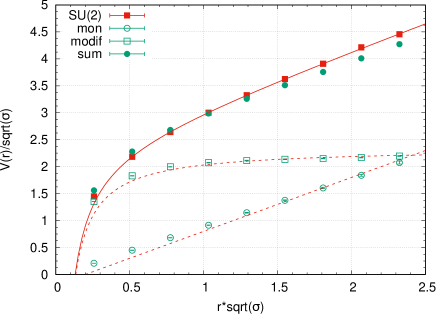
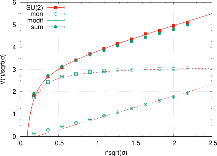
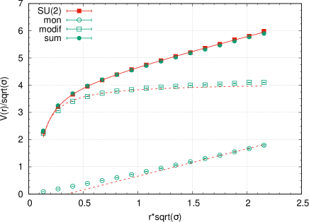
Figure 1: Comparison of the nonabelian potential $V(r)$ (filled squares) with the sum $V_{mod}(r)+V_{mon}(r)$ (filled circles) for $\beta=2.4$ (left upper panel), $\beta=2.5$ (right upper panel), $\beta=2.6$ (lower panel). $V_{mod}(r)$ (empty squares) and $V_{mon}(r)$ (empty circles) are also depicted. The solid curve shows the fit to eq. (13). Two dashed curves show its Coulomb and linear terms with adjusted constants.

Table 1: Parameters of the potentials obtained by fits to the function (13)

Potential	$\beta=2.4$		$\beta=2.5$		$\beta=2.6$
	$~{}~{}~{}~{}\sigma a^{2}\qquad$	$\alpha$	$\sigma a^{2}$	$\alpha$	$\sigma a^{2}$	$\alpha$
$V$	0.067(1)	-0.31(1)	0.033(1)	-0.290(4)	0.0184(5)	-0.25(1)
$V_{mon}+V_{mod}$	0.058(1)	-0.27(1)	0.030(1)	-0.27(1)	0.0175(4)	-0.25(1)
$V_{mon}$	0.060(1)	-0.002(1)	0.030(1)	0.015(3)	0.0167(6)	0.06(2)
$V_{mod}$	-	-0.25(1)	-	-0.27(1)	0.002(1)	-0.27(1)

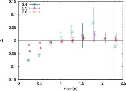
Figure 2: The relative deviation $\Delta(r)$ defined in eq. (14) vs. distance $r$ for three values of the coupling constant $\beta$.

Apart from approach to the continuum limit we studied the question of universality of the decomposition eq. (12). The simulations were made with the tadpole improved action at $\beta=3.4$. The lattice spacing at this coupling is approximately equal to that of the Wilson action at $\beta=2.5$. The result is presented in the Fig. 3 (left). One can see that agreement between $V(r)$ and $V_{mod}(r)+V_{mon}(r)$ is nearly as good as in Fig. 1 for $\beta=2.5$.

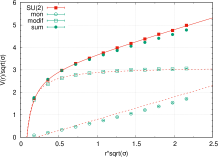
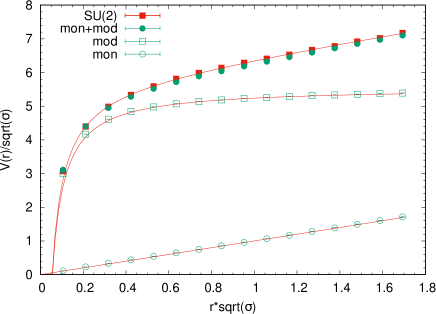
Figure 3: Comparison of the nonabelian potential $V(r)$ (filled squares) with the sum $V_{mod}(r)+V_{mon}(r)$ (filled circles) for improved action at $\beta=3.4$ (left) and for QC₂D (right). $V_{mod}(r)$ (empty squares) and $V_{mon}(r)$ (empty circles) are also shown. The solid curve and dashed curves carry same meaning as in Fig. 1.

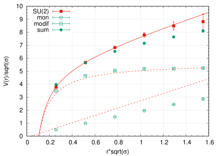
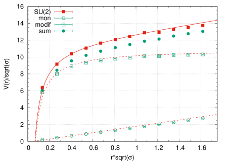
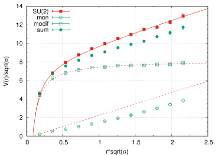
Figure 4: Comparison of the adjoint nonabelian potential $V_{adj}(r)$ (filled squares) with the sum $V_{mod,adj}(r)+V_{mon,q2}(r)$ (filled circles) for Wilson action at $\beta=2.4$ (left, upper panel), $\beta=2.5$ (right, upper panel), $\beta=2.6$ (left, lower panel) and for improved action at $\beta=3.4$ (right, lower panel) . $V_{mod,adj}(r)$ (empty squares) and $V_{mon,q2}(r)$ (empty circles) are also shown. The solid curve and dashed curves carry same meaning as in Fig. 1.

Furthermore, we did the same study in QC₂D on $32^{4}$ lattice with small lattice spacing (for details of simulations see, e.g. Bornyakov:2017txe ). The result is presented in Fig. 3 (right). One can see clearly that approximate decomposition is fulfilled with rather high precision in this case as well.

Next we come to the static potential in the adjoint representation. In this case we check the validity of the relation

$$V_{adj}(r)\approx V_{adj,mod}(r)+V_{mon,q2}(r)$$ (15)

Our numerical results for three lattice spacing for the Wilson action and for one lattice spacing for the improved action are presented in Fig. 4. In this case the precision of our results is lower still it is seen that the relation (15) is satisfied quite well. The signature of improving the agreement between lhs and rhs in (15) with decreasing lattice spacing is also seen although this should be checked in more precise measurements.

IV Conclusions

We studied the decomposition of the static potential in the fundamental and adjoint representations into the linear term produced by the monopole (Abelian) gauge field $U_{mon}(x)$ and the Coulomb term produced by the monopoleless nonabelian gauge field $U_{mod}(x)$. We confirm the results of Ref. Bornyakov:2005hf and improve them in a few respects. First, we made computations with varying lattice spacing and found that in both representations the agreement becomes better with decreasing lattice spacing. Our results suggest that the relations (12) and (15) become exact in the continuum limit. Further work is needed to provide more evidence for this conclusion. Second, we checked that the decomposition is valid also in the case of improved lattice action and in the theory with quarks. These results make it even more interesting to check this decomposition in the case of $SU(3)$ gauge group.

There are few conclusions to be drawn from the decomposition (12). It suggests that the monopole part $U_{mon}(x)$ is responsible for the classical part of the hadronic string energy while the monopoleless part $U_{mod}(x)$ produces the fluctuating part of that energy, i.e. while at small distances $U_{mod}(x)$ should reproduce the perturbative results at large distances it contributes to the nonperturbative physics.

- [1] V. G. Bornyakov, M. I. Polikarpov, G. Schierholz, T. Suzuki and S. N. Syritsyn, Nucl. Phys. B Proc. Suppl. 153, 25-32 (2006) [arXiv:hep-lat/0512003 [hep-lat]].
- [2] T. Suzuki and I. Yotsuyanagi, Phys. Rev. D 42 (1990) 4257.
- [3] S. Hioki, S. Kitahara, S. Kiura, Y. Matsubara, O. Miyamura, S. Ohno and T. Suzuki, Phys. Lett. B 272, 326 (1991) [Erratum-ibid. B 281, 416 (1992)].
- [4] G. S. Bali, V. Bornyakov, M. Muller-Preussker and K. Schilling, Phys. Rev. D 54 (1996) 2863.
- [5] V. Bornyakov and M. Muller-Preussker, Nucl. Phys. Proc. Suppl. 106, 646 (2002).
- [6] N. Sakumichi and H. Suganuma, Phys. Rev. D 90 (2014) no.11, 111501 doi:10.1103/PhysRevD.90.111501 [arXiv:1406.2215 [hep-lat]].
- [7] A. S. Kronfeld, M. L. Laursen, G. Schierholz and U. J. Wiese, Phys. Lett. B 198, 516 (1987).
- [8] G. ’t Hooft, Nucl. Phys. B 190 (1981) 455.
- [9] H. Shiba and T. Suzuki, Phys. Lett. B 333, 461 (1994).
- [10] J. D. Stack, S. D. Neiman and R. J. Wensley, Phys. Rev. D 50, 3399 (1994).
- [11] M. N. Chernodub and M. I. Polikarpov, in ”Confinement, Duality and Non-perturbative Aspects of QCD”, p.387, Plenum Press, 1998, hep-th/9710205; R. W. Haymaker, Phys. Rept. 315 (1999) 153.
- [12] G. ’t Hooft, in High Energy Physics, ed. A. Zichichi, EPS International Conference, Palermo (1975); S. Mandelstam, Phys. Rept. 23, 245 (1976).
- [13] O. Miyamura, Phys. Lett. B 353, 91 (1995).
- [14] S. Kitahara, O. Miyamura, T. Okude, F. Shoji and T. Suzuki, Nucl. Phys. B 533, 576 (1998)
- [15] P. de Forcrand and M. D’Elia, Phys. Rev. Lett. 82, 4582 (1999) [arXiv:hep-lat/9901020].
- [16] J. Smit and A. van der Sijs, Nucl. Phys. B 355, 603 (1991).
- [17] G. Parisi, R. Petronzio and F. Rapuano, Phys. Lett. B 128, 418 (1983).
- [18] M. Albanese et al. [APE Collaboration], Phys. Lett. B 192, 163 (1987).
- [19] G. I. Poulis, Phys. Rev. D 54, 6974 (1996)
- [20] V. G. Bornyakov, V. V. Braguta, E. M. Ilgenfritz, A. Y. Kotov, A. V. Molochkov and A. A. Nikolaev, JHEP 03 (2018), 161 doi:10.1007/JHEP03(2018)161 [arXiv:1711.01869 [hep-lat]].
- [21] V. Bornyakov and M. Muller-Preussker, Nucl. Phys. B Proc. Suppl. 106 (2002), 646-648 doi:10.1016/S0920-5632(01)01803-5 [arXiv:hep-lat/0110209 [hep-lat]].