PEng4NN: An Accurate Performance Estimation Engine for Efficient Automated Neural Network Architecture Search

Abstract

Neural network (NN) models are increasingly used in scientific simulations, artificial intelligence, and other high performance computing (HPC) fields to extract knowledge from datasets. Each dataset requires tailored NN model architecture, but designing individual structures by hand is a time-consuming and error-prone process. Neural architecture search (NAS) automates the design of NN architectures. NAS attempts to find well-performing NN models for specialized datsets, where performance is measured by key metrics that capture the NN capabilities (e.g., accuracy of classification of samples in a dataset). Existing NAS methods are still resource intensive, especially when searching for highly accurate models for larger and larger datasets.

To address this problem, we propose a performance estimation strategy that reduces the resources for training individual NNs and increases NAS throughput without jeopardizing accuracy. We implement our strategy via an engine called PEng4NN that plugs into existing NAS methods; in doing so, PEng4NN predicts the final training accuracy of NNs early in the training process, informs the NAS of NN performance, and thus enables the NAS to terminate training NNs early. We assess the effectiveness of our engine on three diverse datasets (i.e., CIFAR-100, Fashion MNIST, and SVHN). By reducing the quantity of training epochs needed, our engine achieves substantial throughput gain; on average, our engine saves 61% to 82% of the training epochs needed, increasing throughput by a factor of 2.5 to 5 compared to a state-of-the-art NAS method. We achieve this gain without compromising accuracy, as we demonstrate with two key outcomes. First, across all our tests, between 74% and 97% of the ground truth best models lie in our set of predicted best models. Second, the accuracy distributions of the ground truth best models and our predicted best models are comparable, with the mean accuracy values differing by at most .7 percentage points across all tests.

I Introduction

Neural networks are powerful models that are increasingly leveraged in traditional HPC-oriented fields like scientific simulations and new research areas such as high-performance artificial intelligence and high-performance data analytics. However, finding a suitable neural network architecture is a time-consuming, data-dependent process involving several rounds of hyperparameter selection, training, validation, and manual inspection.

Recent works have proposed methods to automate the design of neural networks, including neural architecture search (NAS) strategies to find near-optimal models for a given dataset. NAS involves selecting neural network (NN) models from the search space, training them on the target dataset, evaluating their performance, and using information about NN performance to select new NNs from the search space. This process is computationally intensive and time-consuming for even a single network, and it is typically conducted in an iterative manner, which increases the need for computing power even further.

In order to improve the throughput and efficiency of NAS, NN models can be analyzed to estimate their performance and establish early termination criteria or steer searching mechanisms. Limited research exists in the area of NN performance estimation and early termination criteria, and such methods are often directly integrated into a particular NAS implementation. In this paper, we propose PEng4NN, a performance estimation engine that predicts fully-trained network accuracy early in the training process. Crucially, PEng4NN decouples the search and estimation strategies in state-of-the-art NAS methods: it plugs into existing NAS workflows and outputs performance estimates for the NN models. This information can be leveraged by the NAS to redirect computational resources from training, thus increasing the throughput of the NAS and allowing it to explore more candidate models.

The contributions of this work are:

1. The definition of a core accuracy predictive function that models the accuracy of an NN independently of its architecture and the dataset it aims to classify.

2. The design of a performance estimation strategy agnostic to the NAS method and dataset of choice, capable of accurately inferring the performance of a given NN model in fewer training epochs than comparable state-of-the-art methods.

3. The implementation of this strategy as PEng4NN, a fully decoupled performance estimation engine that can plug into existing NAS engines for classification problems.

4. A systematic characterization of widely accepted benchmark datasets for NN training and validation (i.e., CIFAR-100, Fashion MNIST, and SVHN).

5. An evaluation of PEng4NN on the characterized benchmark datasets, including analysis of our engine’s gain and accuracy.

II Limitations of Neural Architecture Search

Neural networks (NN) are powerful and flexible models that can be tailored to many complex learning tasks like speech and natural language processing, image classification, and even multidimensional scientific problems. Despite their success, NNs are still hard to design manually and they must be tuned for each specific dataset. Recent works aim to automate the design of NN for a given dataset by conducting a neural architecture search (NAS) that selects the number, type, and sequence of layers, and chooses the hyper-parameters that describe how each layer functions. In current literature there are several strategies to conduct NAS, including random searches, grid searches, hyper-parameter sweeps, reinforcement learning, evolutionary optimization, gradient-based optimization, and bayesian optimization [1]. Most of these strategies are implemented as search engines that incorporate on-the-fly learning to improve the generated models iteratively. The aggregated load of training all the NNs in the vast search space makes NAS a computationally intensive problem that requires a high-throughput approach, especially in the early stages of NAS in which up to 88% of NN fail to ever learn [2]. Consequently, scientists must either allocate significant time on the largest compute resources available (in the range of tens of thousands of GPU hours [3]) or make assumptions about the models to simplify the search.

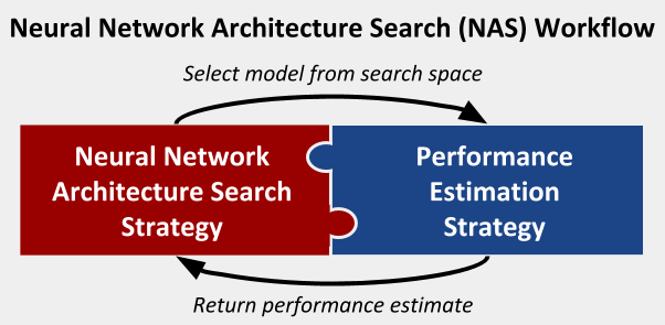
To alleviate this issue, NAS can be supported by performance estimation strategies that provide information (e.g., accuracy or loss) for a given model trained on a specific dataset. These estimates enable the NAS to truncate the training process, compare partially-trained NNs, and steer the search towards models that yield better performance. As a result, performance estimation strategies can improve the efficiency and throughput of the NAS. This results in an overall NAS workflow in which the NAS strategy selects an NN model from the search space for a specific dataset and feeds this model to the performance estimation strategy, which returns a performance estimate that can be leveraged by the NAS. Figure 1 shows the tightly-coupled vision of this NAS workflow as found in the literature [1]. This yields that a performance estimation strategy is tailored for a specific NAS method, which imposes restrictions to the generalization of the performance estimation strategy for different NAS engines. A coupled design also prevents conducting optimizations in the resource allocation for each component of the workflow, their orchestration, and the mechanisms to exchange data efficiently amongst them. All of these limitations can reduce the efficiency and throughput of the NAS workflow as a whole. This work addresses these limitations by designing a decoupled performance estimation strategy that we implement as the PEng4NN performance estimation engine. By decoupling the NAS from PEng4NN, we can plug our engine into diverse NAS applied to different datasets.

Figure 1: Overview of current NAS workflows and their tightly-coupled relationship between the search and performance estimation strategies.

III Performance Estimation Engine (PEng4NN)

Figure 2: Overview of PEng4NN, our solution of a decoupled performance estimation engine that, given an input NN model provided by the NAS, outputs a performance estimate that can be leveraged by the NAS.

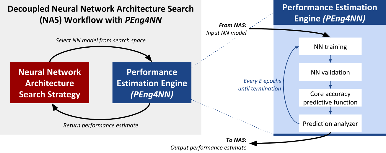
Our performance estimation strategy relies on a fully decoupled NAS and NN performance estimation, as shown in Figure 2. In doing so, we pursue a strategy that is agnostic to the NAS methods and datasets. We implement this strategy in PEng4NN, our fully decoupled performance estimation engine. PEng4NN augments NAS strategies to improve their throughput and efficiency. Each time the NAS selects an NN model, it first passes that model to PEng4NN. The performance estimation engine iteratively executes a four-step process depicted in Figure 2. PEng4NN begins each iteration by training and validating the NN. It then constructs a core accuracy predictive function based on the NN’s validation performance. PEng4NN passes the prediction derived from this function to the prediction analyzer that determines whether a stable performance estimate was found. With this information, PEng4NN decides whether to output a final estimate or continue the iterative process. The following subsections describe in detail the components of PEng4NN.

III-A NN training and validation

The dataset of interest for the classification problem is divided into a training set and a validation set. At each iteration, PEng4NN trains a given NN model $M$ on the training data for a constant number of epochs, $E$, where an epoch means one cycle through the training set. The value of parameter $E$ is user-defined. In all of our tests, we let $E=0.5$, meaning that PEng4NN trains the NN for 0.5 epochs at each iteration (i.e., the NN is trained on half the training data). PEng4NN then validates the NN and calculates its classification accuracy ($a_{V}$) and loss ($l_{V}$) for the validation set at the current epoch ($e$). Note that we select a batchsize and truncate our datasets to be divisible by the batchsize. As a result we ensure we can train for precisely 0.5 epochs.

III-B Core accuracy predictive function

We define the predictive function that we fit to the NN accuracy data across epochs, and we analytically determine bounds and initial values for the predictive function’s parameters. Then, we describe how we leverage Sci-Py’s optimize.curve_fit method (Curve Fit) to fit our chosen function to the historic accuracy data of a given NN model. Finally, we show how we use the fitted predictive function to determine a maximum accuracy prediction for the NN at each iteration of the engine.

III-B1 Defining the function

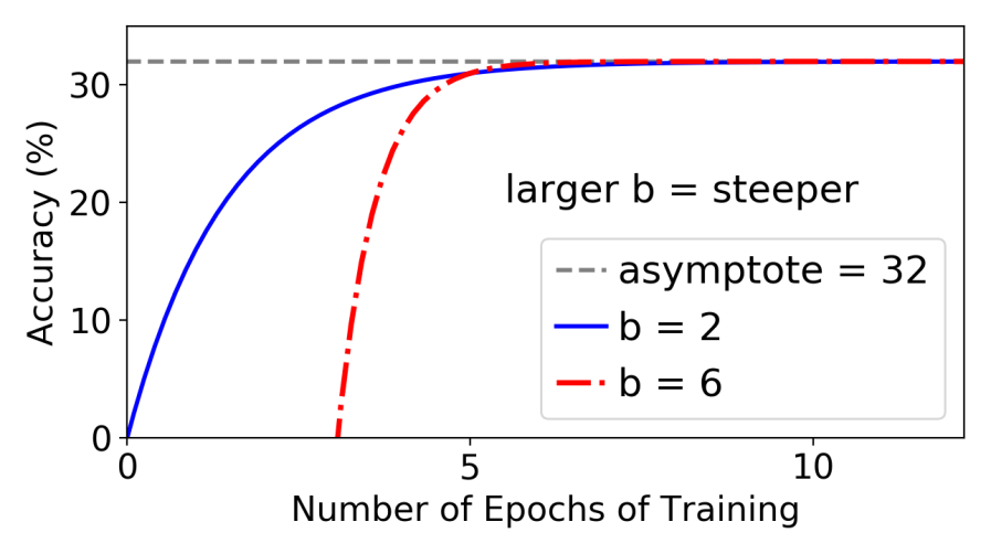
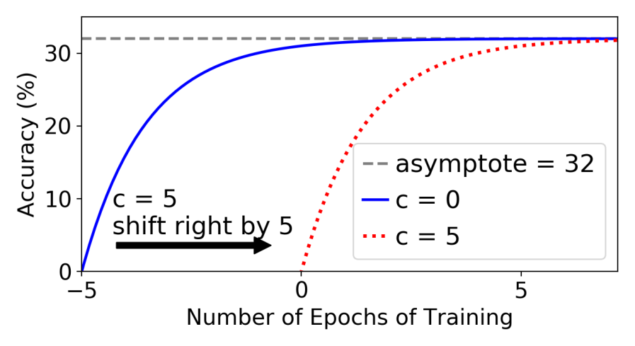
We hypothesize that NN accuracy curves can be modeled with functions of the form $f(x)=a-b^{(c-x)}$. Empirical observation suggests that the accuracy curves of NNs tend to be concave down and increasing, with a horizontal asymptote that the accuracy values approach; the family of functions $f(x)=a-b^{(c-x)}$ shares these properties. The function parameter $a$ describes the horizontal asymptote; the parameter $b$ controls steepness of the curve/corner; the parameter $c$ denotes a horizontal shift. Figure 3a depicts a sample function with different values for $b$: $f(x)=32-b^{(5-x)}$, with a solid blue line for $b=2$ and a dashed red line for $b=6$. The dashed red line with the larger $b$ value is the steeper curve, illustrating that larger values for the parameter $b$ correspond to steeper curves. Figure 3b depicts a sample function with different values for $c$: $f(x)=32-2^{(c-x)}$, with a solid blue line for $c=0$ and a dotted red line for $c=5$. The dotted red line with $c=5$ is shifted right by 5 points as compared to $c=0$, illustrating that the parameter $c$ denotes a horizontal shift.

(a) $f(x)=32-b^{(5-x)}$

(b) $f(x)=32-2^{(c-x)}$

Figure 3: Sample function with different values for parameters $b$ and $c$

III-B2 Bounding and initializing the function

We define bounds for the three function parameters $a$, $b$  and $c$.

Bounding $a$: The maximum accuracy prediction (defined by parameter $a$) should be strictly greater than 0% and at most 100%. In many cases, the accuracy of an NN increases very quickly at first, and the rate of improvement decreases over epochs.

During early iterations of PEng4NN Curve Fit has limited datapoints for fitting the function. We observe empirically for some NNs that during these first steps Curve Fit expects unreasonable accuracy growth because it sees only the steepest portion of the accuracy curve with the largest rate of increase. Then, if $a$ is unbounded, Curve Fit selects a larger value for $a$ than is reasonable (i.e., larger than 100%). We want to distinguish this scenario from NNs that are simply very accurate. If we bound $a$ by 100, then Curve Fit may predict 100% accuracy in both situations described above. Instead, we allow $a$ to be slightly larger than 100. This enables us to disallow convergence if the value of $a$ is greater than 100 (i.e., in the case that Curve Fit has seen only the steepest part of the curve and predicts unreasonable accuracy growth). In PEng4NN, we bound $a$ by $0.5\leq a\leq 102.5$ and initialize it with $a=10$.

Bounding $b$: The function is undefined at any non integer powers if $b<0$; therefore, $b$ must be strictly positive. Furthermore, if $b<1$, then the function no longer has the desired shape; instead of increasing up to a horizontal asymptote as $x$ increases, the function approaches negative infinity as $x$ increases. Thus, $b\geq 1$. In PEng4NN, we bound $b$ by $1\leq b\leq\infty$ and initialize it with $b=1.001$.

Bounding $c$: The parameter $c$ represents a horizontal shift of the function. We begin by proving that any horizontal shift to the left (that is, a shift by $c$ where $c$ is negative) implies that $f(1)\geq a-1$.

Consider the function $f(x)=a-b^{(c-x)}$. If $c<0$, it follows that $f(1)=a-b^{i}$, where $i<-1$, or $f(1)=a-\frac{1}{b^{j}}$, where $j>1$. Then, because $b\geq 1$, it follows that $f(1)\geq a-1$.

Before passing the validation accuracy values per epoch to Curve Fit, we rescale the $x$ values so that the initial value for $x$ is 1, meaning that the corresponding epoch values will be rescaled to start at 1. Then, $f(1)\geq a-1$ means that the initial accuracy is within 1% of the maximum accuracy; in other words, the NN accuracy improves by only 1% throughout training. Such behavior is modeled by a flat line with $b=1$, in which case the value of $c$ has no effect on the function. Because of this observation, we conclude that horizontal shifts to the left are not needed, and hence $c\geq 0$. In PEng4NN, we bound $c$ by $0\leq c\leq\infty$ and initialize it with $c=100$.

III-B3 Fitting the function to predict accuracy

Algorithm 1 shows the internal procedure in the core accuracy predictive function. Given an NN model $M$, the procedure takes as input the current training epoch ($e$), the history of validation performance and predicted accuracy as a list ordered by epoch ($\mathcal{H}$), the validation accuracy ($a_{V}$) and loss ($l_{V}$) at epoch $e$, and the predictive function $f(x)=a-b^{(c-x)}$ that is bounded and initialized with the values specified in the previous section.

The first step in our core predictive procedure is the creation of a new tuple of performance metrics for $M$ at the specified epoch ($h_{e}$). This tuple is inserted in the performance history $\mathcal{H}$ for $M$ (Line 5) so that it is taken into consideration as a new datapoint for the Curve Fit method. The rest of the steps required to fit the function $f$ only take place if there are enough datapoints to conduct the Curve Fit method. In this case $f$ is an exponential function, thus we need at least $C_{min}=3$ datapoints in $\mathcal{H}$ to proceed (Line 6).

Recall that the constant number of training epochs per iteration of PEng4NN ($E$) is user-defined (see Sec. III-A). We rescale $\mathcal{H}$ as a new list $\mathcal{H}^{\prime}$ in which the first epoch value is 1 (Line 7), since this enables us to assign general bounds for the parameters $a$, $b$, and $c$ that do not depend on the value of $E$. For example, if the NN is validated every half epoch, the first epoch value is 0.5, so $\mathcal{H}$ is rescaled by multiplying by 2 every value of $e$ in the list. Then we feed $\mathcal{H}^{\prime}$ to SciPy’s optimize.curve_fit method to find the function $f$ that best fits the historic accuracy data for the NN model (Line 8). We define the maximum accuracy prediction $a_{P}$ given by the predictive function $f$ as the value of the parameter $a$ that results from Curve Fit. We update this value $a_{P}$ in the performance tuple for the current epoch ($h_{e}$) so that it is reflected in the performance history (Line 10).

As a result of the core accuracy predictive function, we output the updated history of validation performance and accuracy predictions ($\mathcal{H}$) for further analysis.

III-C Prediction analyzer

Each time the core accuracy predictive function receives a new validation performance measurement for an NN model $M$ at epoch $e$, it generates a maximum accuracy prediction $a_{P}$ that is appended to the history of measured and predicted values $\mathcal{H}$. The fitted function and the associated $a_{P}$ vary from one iteration to the next because new performance measurements are appended to $\mathcal{H}$. The goal of the prediction analyzer is to determine whether the performance estimates for $M$ have converged to a stable value, which we denote by $A_{P}$.

TABLE I: Symbols for accuracy predictive function algorithm.

Symbol	Definition
$M$	NN model identifier
$e$	Current epoch in which the prediction will be calculated
$a_{V}$	Validation accuracy from NN validation component
$l_{V}$	Validation loss from NN validation component
$a_{P}$	Predicted accuracy
$\mathcal{H}$	Ordered list of $<M,e,a_{V},l_{V},a_{P}>$ tuples, each representing the validation accuracy $a_{V}$ and loss $l_{V}$ of an NN $M$ at a specific epoch $e$, plus the accuracy prediction $a_{P}$
$f$	Initial function for the Curve Fit method
$C_{min}$	Minimum cardinality of the dataset $f$ will be fitted to
$a$	Horizontal asymptote for the fitted function at epoch $e$
$b$	Steepness of the fitted function at epoch $e$
$c$	Horizontal shift of the fitted function at epoch $e$

Algorithm 1 Procedure for accuracy predictive function.

1:Current training epoch ($e$); history of validation performance and predicted accuracy ($\mathcal{H}$); validation performance at epoch $e$ (i.e., accuracy, $a_{V}$, and loss, $l_{V}$); function to fit ($f$) and minimum required cardinality ($C_{min}$)

2:History of validation performance and predicted accuracy ($\mathcal{H}$), updated with the latest prediction $a_{P}$

3:procedure Predictor($e$, $\mathcal{H}$, $a_{V}$, $l_{V}$, $f$)

4:    $h_{e}\leftarrow<M,e,a_{V},l_{V},0>$

5:    $\mathcal{H}\leftarrow insert(h_{e})$

6:    if $|\mathcal{H}|\geq C_{min}$ then

7:         $\mathcal{H}^{\prime}\leftarrow rescale\_epochs(\mathcal{H})$

8:         $a,b,c\leftarrow optimize.curve\_fit(\mathcal{H}^{\prime},f)$

9:         $a_{P}\leftarrow a$

10:         $\mathcal{H}\leftarrow update\_prediction(\mathcal{H},h_{e},a_{P})$     

11:    return $\mathcal{H}$

We describe the prediction analyzer component of PEng4NN by first defining the parameters that control the prediction analysis. We then describe the conditions to detect convergence and show how we compute the output estimate.

III-C1 Parameterizing the analysis

We determine six parameters to control the behavior of the prediction analyzer and its convergence criteria:

• $N$, the number of most recent accuracy predictions to consider. We use $N=3$.

• $E$, the number of epochs per iteration. We use $E=0.5$.

• $e_{max}$, the maximum number of epochs we allow an NN to train. We use $e_{max}=20$.

• $t$, the threshold describing how much variability is small enough to establish convergence and report a final performance estimate. We use $t=0.5$.

• $LOSS$, a boolean describing whether or not to enable a validation loss check in the analyzer. It is useful for datasets on which an NN’s accuracy may be noisy or slow to increase, more commonly encountered in unbalanced datasets. We use $LOSS=$ true for unbalanced datasets and $LOSS=$ false otherwise. When the loss check is enabled, it is only activated if the latest accuracy prediction indicates that the given NN is not performing better than guessing or has not learned more than a single class (for example, accuracy of 10% in the case of a balanced 10 class dataset). We call such an accuracy prediction a never-learn prediction.

• $L$, the number epochs to consider in the loss check. We use $L=5$.

These parameters, summarized in Tab. II, constitute part of the input arguments for the prediction analyzer procedure and can be adjusted in PEng4NN to tune the overall iterative process.

III-C2 Analyzing the convergence of the predictions

Algorithm 2 shows the internal procedure in the prediction analyzer. Given an NN model $M$, the procedure takes as input the current training epoch ($e$), the history of validation performance and predicted accuracy ($\mathcal{H}$), and the six configuration parameters described above. We first check if we have reached the minimum number of epochs to assess convergence (Line 6). If not, this means the number of tuples in $\mathcal{H}$ is not sufficient to analyze whether the predictions are stable, so we must continue training. On the other hand, if we reached the maximum number of training epochs ($e_{max}$), we return the maximum observed validation accuracy $a_{V}$ (Line 7) with convergence status false.

We assume that, if convergence is achieved, the final performance estimate ($A_{P}$) corresponds to the accuracy predicted by the predictive function in the current epoch ($a_{P}$) (Line 8). We define three conditions for reaching convergence:

• Condition 1: The most recent maximum accuracy prediction ($A_{P}$) must be less than or equal to 100%. Otherwise, the prediction is not valid to establish convergence (Line 9). Recall that parameter $a$ of the fitted function determines the max accuracy prediction. Recall also that we allow Curve Fit to choose $a$ larger than 100 so that we can detect if Curve Fit is predicting unreasonable accuracy growth. This condition ensures that we have a realistic value for $A_{P}$.

• Condition 2: The $N$ most recent maximum accuracy predictions are all within the threshold $t$ of their mean (Line 10). In other words, for each of the $N$ most recent predictions $p_{i}$, it checks if $mean-t\leq p_{i}\leq mean+t$.

• Condition 3: If the loss check is activated (Line 11) and the most recent maximum accuracy prediction $a_{P}$ is a never-learn prediction (Line 12), then the minimum validation loss $l_{V_{min}}=min\{l_{V}\in\mathcal{H}\}$ has not decreased for at least $L$ epochs (Line 13). This condition ensures that the NN is not merely learning slowly or irregularly, as can be the case especially with unbalanced datasets. On the contrary, if the accuracy is not increasing, and the validation loss is not decreasing, this indicates that the NN is likely not continuing to learn.

TABLE II: Symbols for prediction analyzer algorithm.

Symbol	Definition
$e$	Current epoch in which the predictions are analyzed
$\mathcal{H}$	Ordered list of $<M,e,a_{V},l_{V},a_{P}>$ tuples, each representing the validation accuracy $a_{V}$ and loss $l_{V}$ of an NN $M$ at a specific epoch $e$, plus the accuracy prediction $a_{P}$
$N$	Number of most recent accuracy predictions to consider in the analysis. We use $N=3$
$E$	Number of epochs per iteration. We use $E=0.5$
$e_{max}$	Maximum number of epochs to train. We use $e_{max}=20$
$t$	Maximum performance variability allowed for convergence. We use $t=0.5$
$LOSS$	Indicates whether the loss check is enabled
$L$	Number of epochs to consider in the loss check. We use $L=5$
$l_{V_{min}}$	Minimum validation loss observed
$A_{P}$	Most recent accuracy estimate for the NN model $M$ on convergence

Algorithm 2 Procedure for prediction analyzer.

1:Current training epoch ($e$); history of validation performance and predicted accuracy ($\mathcal{H}$); configuration parameters

2:Convergence status (converged)

3:Performance estimate (predicted accuracy ($A_{P}$) if convergence is achieved; maximum observed validation accuracy ($a_{V}$) if $e_{max}$ is reached)

4:procedure Analyzer($e$, $\mathcal{H}$, $N$, $E$, $e_{max}$, $t$, $LOSS$, $L$)

5:    converged $\leftarrow$ false

6:    if $e\leq N\cdot E$ then exit     

7:    if $e=e_{max}$ then return $max\{a_{V}\in\mathcal{H}\}$     

8:    $A_{P}\leftarrow a_{P}$ from $\mathcal{H}$ in epoch $e$

9:    if $A_{P}>100$ then exit     

10:    if last $N$ $a_{V}\in\mathcal{H}$ are within $t$ then

11:         if $LOSS$ is true then

12:             if $A_{P}$ is never-learn then

13:                 if last $L\cdot E$ $l_{V}\in\mathcal{H}\geq l_{V_{min}}$ then

14:                     converged $\leftarrow$ true                               

15:         else converged $\leftarrow$ true              

16:    if converged is true then return $A_{P}$

17:    else exit     

There are two possible outcomes based on these conditions. If the conditions are all true, it means the prediction has converged. In this case, the performance estimation engine outputs $A_{P}$ with convergence status true (Line 16). On the other hand, if any one of the conditions is not met, and the NN has not yet trained for $e_{max}$ epochs, the procedure ends with convergence status false (Line 17).

Based on the output of the prediction analyzer, we can establish the termination criteria for PEng4NN. If a performance estimate is returned, PEng4NN terminates and sends this value to the NAS. This can occur in two scenarios: either we reached convergence and the output is $A_{P}$, or we reached $e_{max}$ and the output is $max\{a_{V}\in\mathcal{H}\}$. We can distinguish these cases by inspecting the value of the convergence status. On the other hand, if no value is returned, then PEng4NN will begin the next iteration and resume training the NN model.

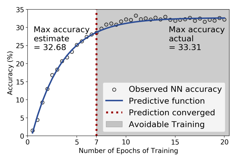
As an example, Figure 4 depicts the end result of this process for one of the NNs we trained on CIFAR-100. The x-axis indicates the number of training epochs, and the y-axis indicates accuracy of the NN. The dotted red line indicates the point at which the prediction converges; this is when our engine outputs the performance estimate and terminates the iterative training process. In this example, our engine terminates the iterative process and outputs the performance estimate after 7 epochs. The predictive function from the final iteration is graphed, along with validation accuracy datapoints for the NN across $e_{max}=20$ epochs for comparison. Note that only the accuracy values from the first 7 epochs were used to fit the predictive function and estimate performance.

Figure 4: Example of the estimate and predictive function given by PEng4NN for a neural network trained on CIFAR-100

IV Evaluation

We describe our experimental setup and evaluate our engine to answer two key questions: (i) “What savings are gained by our approach?” and (ii) “How accurate are the predictions made by our approach?”

IV-A Experimental Setup

IV-A1 Dataset Characterization

To the best of our knowledge, there is no systematic characterization of datasets used in ML evaluations. This makes the assessment of the generality and applicability of a method in the area of NN research a case-driven discussion [4, 5, 6, 7, 8, 9] that is also found in works tackling the problem of evolutionary NN design [10, 11]. We characterize three of the most commonly used datasets (i.e., CIFAR-100, F-MNIST, and SVHN) that act as benchmarks in the evaluation of novel methods and techniques for NN. Four key attributes demonstrate the diverse nature of these datasets—number of samples, number of classes, number of image color channels, and sample size [12], plus an additional aspect of the internal balancing of the sample distribution per class, which is known to affect the performance of NNs in terms of accuracy [13]. Table III summarises these attributes and shows a sample from each dataset. We evaluate PEng4NN with these datasets that we describe below.

CIFAR-100: This dataset was introduced in 2009 [14] as a subset of the 80 Million Tiny Images dataset [15], aimed towards improving tasks of unsupervised training of deep generative models. It is still one of the most popular benchmarks in the field of computer vision due to the manageable size of the dataset, the resolution of its images, and its challenges for NN models [16, 17, 18].

Fashion MNIST (F-MNIST): This dataset [19] serves as a replacement for the original MNIST dataset comprising ten classes of handwritten digits [20]. It shares the same image and dataset size, data format, and structure of training and testing splits with MNIST, making it a popular benchmark for NN models targeting computer vision problems [21, 22, 23].

SVHN: Like MNIST, SVHN [24] contains digits, but in this case they are obtained from real-world house numbers, thus contain color information, various natural backgrounds, overlapping digits, and other distracting features. These characteristics make SVHN a more difficult dataset compared to MNIST, which makes SVHN a very popular benchmark for NNs [25].

TABLE III: Characterization of CIFAR-100, F-MNIST, and SVHN.

		CIFAR-100	F-MNIST	SVHN
Number of samples		60,000	70,000	600,000
	Training set	50,000 (83%)	60,000 (86%)	373,257 (62%)†
	Validation set	10,000 (17%)	10,000 (14%)	26,032 (4%)†
Number of classes		100	10	10
	Samples per class	600	7,000	6,500 to 19,000
	Balanced	Yes	Yes	No
Number of channels		3	1	3
Sample size (pixels)		32$\times$32	28$\times$28	32$\times$32

^†SVHN also contains 531,131 samples that can be used as additional training data, which we did not use in our evaluation.

IV-A2 Neural Network Generation

We train a set of diverse NNs on each of these datasets, where each NN is generated with randomly selected parameters. We randomize the kernel, stride, and padding for convolutional layers (in ranges $[1,5]$, $[1,5]$, and $[0,5]$, respectively) and pooling layers (in ranges $[1,5]$, $[1,pool~{}kernel]$, and $[1,pool~{}kernel/2]$, respectively).We also randomize the number of filters of each hidden convolutional layer (allowing a maximum of 400 for any given layer), number of convolutional layers (between 1 and 10), and the learning rate of the network (between $10^{-6}$ and $1+10^{-6}$). We add a pooling layer after each convolutional layer, and two fully connected layers at the end. Overall, we generate and train a set of 343 NNs on CIFAR-100, 505 NNs on F-MNIST, and 290 NNs on SVHN.

IV-B Performance Estimation Engine Gain

To answer first the question, “What savings are gained by our approach?” we utilize two metrics—number of training epochs saved and throughput gain—for each of the three datasets. We compare the gain to state-of-the-art predictions using MENNDL [26].

(a) CIFAR-100

(b) F-MNIST

(c) SVHN

Figure 5: Percentage of training epochs saved.

IV-B1 Training Epochs Saved

We compare the epoch at which PEng4NN terminates the training of each NN model to the epoch at which MENNDL terminates training of that model using its built-in early termination criterion. MENNDL trains each NN for a maximum of 20 epochs, terminating training earlier than that if the network’s minimum training loss has not decreased for at least 10 epochs. In contrast, PEng4NN trains each NN for a maximum of 20 epochs, terminating training when the engine’s prediction converges (as in Fig. 4), avoiding additional training.

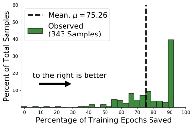
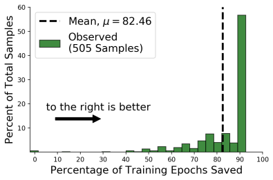
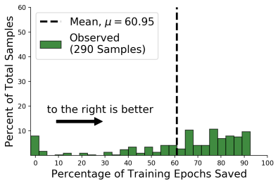
Figure 5 depicts the distribution of NN models according to the percentage of training epochs our method saves for each NN, for our three datasets. Percentage of epochs saved is denoted on the $x$-axis and percent of total NN samples on the $y$-axis. The height of a rectangle denotes the percent of total samples that save the indicated portion of training epochs: taller rectangles to the right indicate that more samples save a larger percentage of epochs (i.e., there is a larger region of avoidable training for these samples). The dashed line indicates the mean percentage of training epochs saved.

For balanced datasets, such as CIFAR-100 and F-MNIST, PEng4NN’s iterative process terminates as soon as the accuracy predictions converge to a value between 0% and 100%. We observe that 40% to 50% of models save more than 90% of the training epochs on CIFAR-100 and F-MNIST (in Fig. 5a and Fig. 5b). For unbalanced datasets, such as SVHN, we describe in Section III an additional condition that we require for prediction convergence for an NN with a never-learn prediction. This delays convergence, and thus we see smaller savings on SVHN (in Fig. 5c). Even so, we observe that nearly 40% of models save 80% or more of the training epochs on SVHN.

For all three datasets, we cut the mean number of training epochs needed to evaluate networks by well over half. We demonstrate respective mean savings of 75%, 82%, and 61% of the training epochs on CIFAR-100, Fashion MNIST, and SVHN, as compared to MENNDL’s early termination criterion (indicated by the dashed lines in Figs. 5a-c).

IV-B2 Throughput Gain

The ability of our performance estimation engine to predict final NN model accuracy early in the training process has immediate implications for NAS. As shown in Figure 5, we can anticipate reducing required training epochs by 60-80% (mean savings depending on data set). The reduction in training epochs for individual NNs increases the number of networks that can be explored and evaluated using the same amount of wall time and compute resources.

For example, on CIFAR-100 in Fig. 5a, the mean savings is approximately 75%; this means PEng4NN evaluates the models in $\frac{1}{4}$ the computation needed by MENNDL. This corresponds to a throughput gain of about $4\times$, allowing $4\times$ the number of networks to be explored with the same computational resources. Similarly, PEng4NN yields a throughput gain of $5\times$ on F-MNIST and $2.5\times$ on SVHN. Exploring more network structures gives the NAS additional opportunity to find better NN models. Alternatively, if the NAS had a fixed problem size (i.e., a set number of models to explore), then one could evaluate those models using fewer computational resources.

IV-C Performance Estimation Engine Accuracy

We now address the second question, “How accurate are the predictions made by our approach?” Recall that the NAS process involves generating models, evaluating their performance, selecting the best models at each step, and using these best models to inform the next generation of models (Section I). PEng4NN reports accuracy estimates for all the generated NNs (see Section III), and the NAS uses these estimates to select the best models. This means it is important for PEng4NN to accurately identify the best NN models from among the set generated by the NAS, as these are the models that are used to create the next generation of models. Thus, in evaluating our prediction accuracy, we compare the ground truth best x% of all our generated models with the predicted best x% of models as identified by PEng4NN. We use PEng4NN’s performance estimates for all the NNs to create a set of our engine’s predicted best x% of models. In our tests, in order to identify the ground truth best x% of models, we allow the NNs to continue training and validating for a full 20 epochs, even after PEng4NN has reported accuracy estimates for them. The models that achieve the highest validation accuracy are the ground truth best models.

We use two metrics to measure the accuracy of PEng4NN’s predictions: overlap, which represents the proportion of the ground truth best models that are also in the set of predicted best models, and accuracy distribution, which depicts the similarity between the NN accuracy values of the ground truth and predicted best models.

IV-C1 Overlap

Figure 6: Overlap metric examples. Left: overlap = 0, Center: overlap = 1/4, Right: overlap = 1

Overlap quantifies how many of the ground truth best models appear in the predicted best models and is defined as $\frac{|\text{ground truth }\cap\text{ prediction}|}{|\text{ground truth}|}$. The overlap value ranges between 0 and 1; the closer to 1, the better. For example, $\text{overlap}=0.8$ would mean that $8/10$ of the ground truth set is overlapping with the prediction set. One could trivially maximize the overlap by simply predicting more best models and allowing additional false positives. We avoid this by ensuring that the number of our predicted best models is always the same as the number of ground truth best models. See Figure 6 for simple illustrative examples of this metric with overlap values equal to 0, 25%, and 100%.

Table IV shows the overlap between PEng4NN’s set of the predicted best $x$% of NN models and the ground truth best $x$% of NN models for different values of $x$ and our three datasets. Across these datasets, for $x$ values ranging from 10% to 30%, the overlap of ground truth best models and predicted best models lies between $0.74$ and $0.97$.

(a) CIFAR-100

(b) F-MNIST

(c) SVHN

Figure 7: Accuracy estimate and actual accuracy for all neural networks, indicating the intersection between ground truth best 20% of models and predicted best 20% of models.

(a) CIFAR-100

(b) F-MNIST

(c) SVHN

Figure 8: Network accuracy distribution of the top 20% of models.
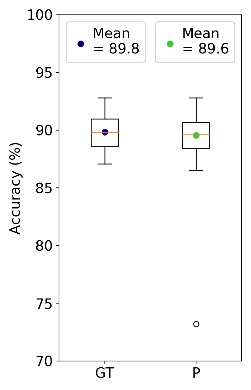
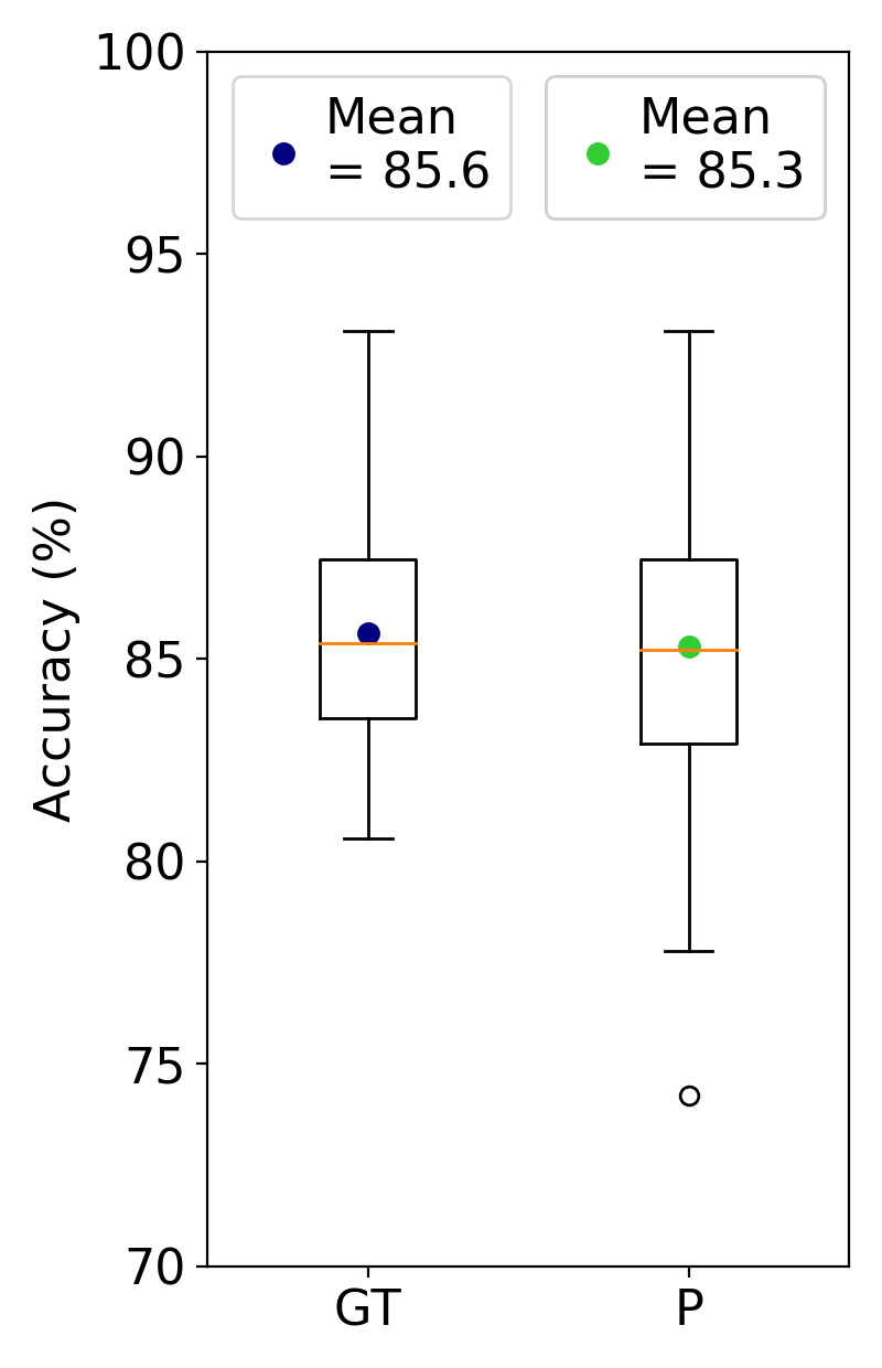
GT = ground truth top 20%, P = predicted top 20%

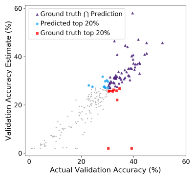
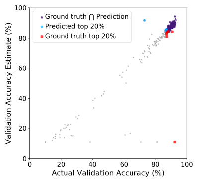
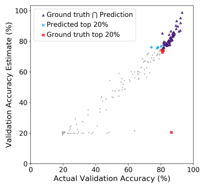
Figure 7 corresponds to the second row of Table IV and depicts, for each dataset, the maximum accuracy estimates and actual maximum accuracy values of all NN models, indicating the ground truth and predicted best 20% and their intersection. Actual maximum accuracy is on the $x$-axis; the estimation engine’s accuracy estimates are on the $y$-axis. The purple triangles depict all NNs that are in both the predicted best 20% of models and the ground truth best 20% of models. The blue circles depict NNs that are in the predicted best 20% of models and not in the ground truth best 20% of models. Last, the red squares depict NNs that are in the ground truth best 20% of models but not in the predicted best 20% of models. Because the $x$-axis indicates actual maximum accuracy, the most accurate models are the furthest to the right of the graph, and the least accurate models are the furthest to the left. We observe that the most accurate models from the set of ground truth best models lie in the intersection with the predicted best models, and the ground truth best models that lie outside of the intersection with the predicted best models tend to be the least accurate ones.

Finally, in the lower left corner of the graph, we see NN models with very low actual accuracy and predicted accuracy; these are models that never learn (i.e. whose accuracy never increases). We see also that there are some outliers parallel to the $x$-axis that have varying levels of actual accuracy but are predicted to have very low accuracy. Validation accuracy for these models does not increase for several epochs. Part of our ongoing work involves studying ways to distinguish between NNs that never learn and NNs that do not learn for many epochs but eventually begin to learn (the outliers).

IV-C2 Accuracy Distribution

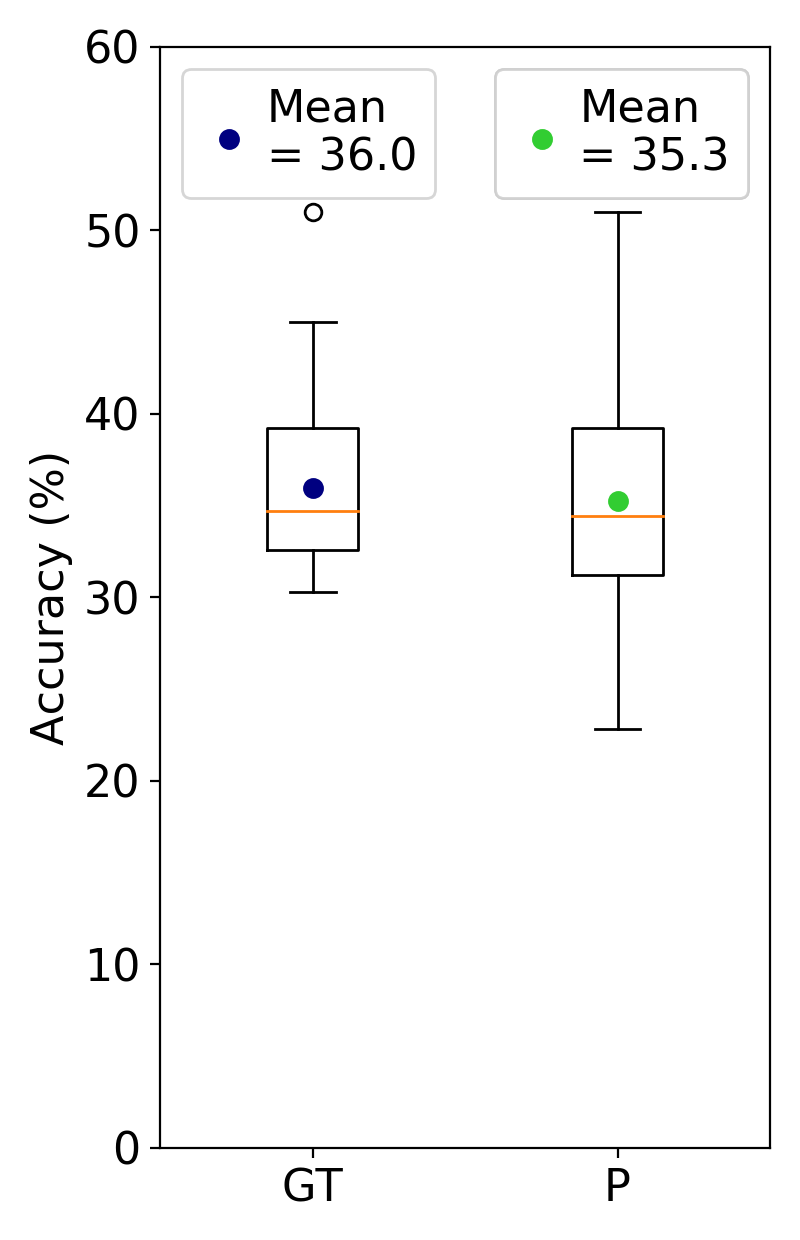
We compare the ground truth and predicted best models with the mean and distribution of the NN accuracy values. Table V shows the difference between the mean accuracy values of the ground truth and predicted best $x\%$ of models for $x=10,20,30$. In all cases, the mean network accuracy of the ground truth best models is very close to the mean network accuracy of the predicted best models: their difference ranges from 0.2 to 0.83 percentage points across all three image datasets and $x$ values.

Figure 8 corresponds to the second row of Table V and depicts the NN accuracy distributions of the ground truth best 20% of models and of the predicted best 20% of models for each of our three datasets. The boxplot shows the 5th, 25th, 50th (red line), 75th and 95th percentiles. The dot represents the mean. Note that the CIFAR-100 figure has a different scale than the F-MNIST and SVHN figures. We observe that for each dataset, the NN accuracy distributions of the ground truth best models and of the predicted best models are comparable. In fact, for all three datasets, the mean NN accuracy for the ground truth best 20% networks lies within 0.7 percentage points of the mean for the predicted best 20% networks. On CIFAR-100, the mean accuracy of the ground truth best models is 36.0%, while the mean accuracy of the predicted best models is 35.3%. On F-MNIST, the mean accuracy of the ground truth best models is 89.8%, while the mean accuracy of the predicted best models is 89.6%. Last, on SVHN, the mean accuracy of the ground truth best models is 85.6%, while the mean accuracy of the predicted best models is 85.3%.

IV-D Discussion

Our experiments show that across diverse datasets, PEng4NN reduces needed training epochs and achieves a throughput gain compared to state-of-the-art NAS while maintaining accuracy in the predicted best models. CIFAR-100, F-MNIST, and SVHN are representative datasets that show diverse values for key dataset attributes (such as samples per class and sample distribution per class). Many of these attributes have implications for dataset classification difficulty and the performance of NNs. The demonstrated gain and accuracy of PEng4NN across all three of these datasets exemplifies our engine’s general applicability for datasets with disparate properties and difficulty.

We observe empirically that unbalanced datasets like SVHN can exhibit additional delay in learning and validation accuracy noise compared to balanced datasets like CIFAR-100 and F-MNIST. To address this, we utilize an additional condition for convergence on unbalanced datasets. If accuracy is not increasing, this condition checks if the NN’s minimum validation loss has decreased within recent epochs. If validation loss has attained a new minimum, this can be an indication that the network is learning slowly, and the condition prevents early convergence in this case.

Furthermore, when studying overlap of the ground truth and predicted best models on all three datasets, we observe outlier models that are predicted to have very low accuracy but have various higher actual accuracy values. These are models that initially do not learn, but eventually learn after a several-epoch delay. Augmenting PEng4NN to differentiate between these outliers and models that never learn is part of our current work.

TABLE IV: Overlap of the actual best $x$% of models and the predicted best $x$% of models for each dataset. Note: the sets of actual and predicted best models have the same size.

	CIFAR-100	F-MNIST	SVHN
10%	0.79	0.74	0.90
20%	0.74	0.87	0.87
30%	0.88	0.97	0.95

TABLE V: Difference in the mean accuracy values of the ground truth best x% of models and predicted best x% of models.

	CIFAR-100	F-MNIST	SVHN
10%	0.83	0.66	0.22
20%	0.70	0.26	0.33
30%	0.58	0.20	0.27

V Related Works

Recent works have proposed different performance estimation strategies. The two most common approaches for truncating training are to train for a fixed but significantly reduced number of epochs (e.g., 20 instead of 100s) [27, 28] or to train until either the maximum accuracy or minimum loss has not improved for a user-specified amount of time (e.g., if the maximum observed accuracy does not improve for 5 epochs). Such methods are commonly included in NN software like Keras. Limited research exists in the area of predicting NN performance [29, 30, 31, 32]. Some methods target hyperparameter search, which involves finding the best hyperparameter configuration for a given human-designed network but does not explore different architectures [29]. Domhan et al. [29] and Klein et al. [30] use probabilistic methods involving computationally expensive Markov Chain Monte Carlo sampling. The approach of Swersky et al. [32] automatically pauses and restarts training of models based on the predicted trajectory of the loss curves. Baker et al. [31] extract features from NNs to use in training a series of regression models to estimate performance.

The solution presented in this paper amplifies these approaches by introducing two key components. The first one is the core accuracy predictive function that provides accurate estimations of the performance of an NN in terms of its maximum accuracy. The second is the prediction analyzer that ensures the stability of these estimations. We design these components to generate performance estimates agnostic to the NN model and the classification dataset in an effective way.

VI Conclusions

This work introduces PEng4NN, an engine that decouples the search and estimation strategies of NAS workflows. It generates accurate performance estimates for NN models and assists NAS strategies in the exploration of the neural architecture search space. Our solution is instrumental for NAS efficiency and throughput: it reduces the training epochs required by 60% to 80% on average, resulting in an increase in the throughput of explored networks of $2.5\times$ to $5\times$. Future work will leverage PEng4NN in state-of-the-art NAS engines to demonstrate how it can increase the efficient interleaving of training, validation, and scientific predictions and analyses in analytics-driven workflows.

References

- [1] T. Elsken, J. H. Metzen, and F. Hutter, “Neural architecture search: A survey,” Journal of Machine Learning Research, vol. 20, no. 55, pp. 1–21, 2019.
- [2] T. Johnston, S. R. Young, D. Hughes, R. M. Patton, and D. White, “Optimizing convolutional neural networks for cloud detection,” in Proceedings of the Machine Learning on HPC Environments, ser. MLHPC’17. New York, NY, USA: Association for Computing Machinery, 2017.
- [3] R. M. Patton, J. T. Johnston, S. R. Young, C. D. Schuman, D. D. March, T. E. Potok, D. C. Rose, S.-H. Lim, T. P. Karnowski, M. A. Ziatdinov et al., “167-pflops deep learning for electron microscopy: from learning physics to atomic manipulation,” in SC18: International Conference for High Performance Computing, Networking, Storage and Analysis. IEEE, 2018, pp. 638–648.
- [4] I. Goodfellow, D. Warde-Farley, M. Mirza, A. Courville, and Y. Bengio, “Maxout networks,” in International conference on machine learning. PMLR, 2013, pp. 1319–1327.
- [5] C.-Y. Lee, S. Xie, P. Gallagher, Z. Zhang, and Z. Tu, “Deeply-supervised nets,” in Artificial intelligence and statistics, 2015, pp. 562–570.
- [6] W. Shi, Y. Gong, and J. Wang, “Improving cnn performance with min-max objective.” in IJCAI, 2016, pp. 2004–2010.
- [7] C. Song, H.-P. Cheng, H. Yang, S. Li, C. Wu, Q. Wu, Y. Chen, and H. Li, “Mat: A multi-strength adversarial training method to mitigate adversarial attacks,” in 2018 IEEE Computer Society Annual Symposium on VLSI (ISVLSI). IEEE, 2018, pp. 476–481.
- [8] X. Han and Q. Dai, “Batch-normalized mlpconv-wise supervised pre-training network in network,” Applied Intelligence, vol. 48, no. 1, pp. 142–155, 2018.
- [9] S. Li, W. Song, H. Qin, and A. Hao, “Deep variance network: An iterative, improved cnn framework for unbalanced training datasets,” Pattern Recognition, vol. 81, pp. 294–308, 2018.
- [10] F. Assunçao, N. Lourenço, P. Machado, and B. Ribeiro, “Denser: deep evolutionary network structured representation,” Genetic Programming and Evolvable Machines, vol. 20, no. 1, pp. 5–35, 2019.
- [11] D. Tan, W. Zhong, X. Peng, Q. Wang, and V. Mahalec, “Accurate and fast deep evolutionary networks structured representation through activating and freezing dense networks,” IEEE Transactions on Cognitive and Developmental Systems, 2020.
- [12] B. Bilalli, A. Abelló, and T. Aluja-Banet, “On the predictive power of meta-features in openml,” International Journal of Applied Mathematics and Computer Science, vol. 27, no. 4, pp. 697–712, 2017.
- [13] J. M. Johnson and T. M. Khoshgoftaar, “Survey on deep learning with class imbalance,” Journal of Big Data, vol. 6, no. 1, p. 27, 2019.
- [14] A. Krizhevsky and G. Hinton, “Learning multiple layers of features from tiny images,” 2009.
- [15] A. Torralba, R. Fergus, and W. T. Freeman, “80 million tiny images: A large data set for nonparametric object and scene recognition,” IEEE transactions on pattern analysis and machine intelligence, vol. 30, no. 11, pp. 1958–1970, 2008.
- [16] L. N. Darlow, E. J. Crowley, A. Antoniou, and A. J. Storkey, “Cinic-10 is not imagenet or cifar-10,” arXiv preprint arXiv:1810.03505, 2018.
- [17] F. Scheidegger, R. Istrate, G. Mariani, L. Benini, C. Bekas, and C. Malossi, “Efficient image dataset classification difficulty estimation for predicting deep-learning accuracy,” The Visual Computer, pp. 1–18, 2020.
- [18] B. Barz and J. Denzler, “Do we train on test data? purging cifar of near-duplicates,” Journal of Imaging, vol. 6, no. 6, p. 41, 2020.
- [19] H. Xiao, K. Rasul, and R. Vollgraf, “Fashion-mnist: a novel image dataset for benchmarking machine learning algorithms,” arXiv preprint arXiv:1708.07747, 2017.
- [20] Y. LeCun, L. Bottou, Y. Bengio, and P. Haffner, “Gradient-based learning applied to document recognition,” Proceedings of the IEEE, vol. 86, no. 11, pp. 2278–2324, 1998.
- [21] K. Meshkini, J. Platos, and H. Ghassemain, “An analysis of convolutional neural network for fashion images classification (fashion-mnist),” in International Conference on Intelligent Information Technologies for Industry. Springer, 2019, pp. 85–95.
- [22] M. Kayed, A. Anter, and H. Mohamed, “Classification of garments from fashion mnist dataset using cnn lenet-5 architecture,” in 2020 International Conference on Innovative Trends in Communication and Computer Engineering (ITCE). IEEE, 2020, pp. 238–243.
- [23] S. Bhatnagar, D. Ghosal, and M. H. Kolekar, “Classification of fashion article images using convolutional neural networks,” in 2017 Fourth International Conference on Image Information Processing (ICIIP). IEEE, 2017, pp. 1–6.
- [24] Y. Netzer, T. Wang, A. Coates, A. Bissacco, B. Wu, and A. Y. Ng, “Reading digits in natural images with unsupervised feature learning,” in NIPS Workshop on Deep Learning and Unsupervised Feature Learning, 2011.
- [25] P. Sermanet, S. Chintala, and Y. LeCun, “Convolutional neural networks applied to house numbers digit classification,” in Proceedings of the 21st International Conference on Pattern Recognition (ICPR2012). IEEE, 2012, pp. 3288–3291.
- [26] T. Johnston, M. Alsulmi, P. Cicotti, and M. Taufer, “Performance tuning of mapreduce jobs using surrogate-based modeling,” Procedia Comput. Sci., vol. 51, no. C, p. 49–59, Sep. 2015.
- [27] E. Real, S. Moore, A. Selle, S. Saxena, Y. L. Suematsu, J. Tan, Q. V. Le, and A. Kurakin, “Large-scale evolution of image classifiers,” in Proceedings of the 34th International Conference on Machine Learning - Volume 70. ICML, 2017, pp. 2902–2911.
- [28] B. Zoph and Q. V. Le, “Neural architecture search with reinforcement learning,” in Proceedings of the 5th International Conference on Learning Representations. ICLR, 2017.
- [29] T. Domhan, J. Springenberg, and F. Hutter, “Speeding up automatic hyperparameter optimization of deep neural networks by extrapolation of learning curves,” in Proceedings of the 24th International Joint Conference on Artificial Intelligence. IJCAI, 2015.
- [30] A. Klein, S. Falkner, J. Springenberg, and F. Hutter, “Learning curve prediction with bayesian neural networks,” in Proceedings of the 5th International Conference on Learning Representations. ICLR, 2017.
- [31] B. Baker, O. Gupta, R. Raskar, and N. Naik, “Accelerating neural architecture search using performance prediction,” in NIPS Workshop on Meta-Learning. NIPS, 2017.
- [32] K. Swersky, J. Snoek, and R. P. Adams, “Freeze-thaw bayesian optimization,” arXiv preprint arXiv:1406.3896, 2014.