Flavor vacuum entanglement in boson mixing

Abstract

Mixing transformations in quantum field theory are non-trivial, since they are intimately related to the unitary inequivalence between Fock spaces for fields with definite mass and fields with definite flavor. Considering the superposition of two neutral scalar (spin-0) bosonic fields, we investigate some features of the emerging condensate structure of the flavor vacuum. In particular, we quantify the flavor vacuum entanglement in terms of the von Neumann entanglement entropy of the reduced state. Furthermore, in a suitable limit, we show that the flavor vacuum has a structure akin to the thermal vacuum of Thermo Field Dynamics, with a temperature dependent on both the mixing angle and the particle mass difference.

I Introduction

The analysis of quantum correlations in the context of particle physics (and in particular for neutrino and meson systems) is currently gaining a rising attention. The initial observation that flavor mixing and oscillations can be associated with (single-particle) entanglement entmix ; entmix2 served as a basis for several studies numecorr ; numecorr2 ; numecorr3 ; numecorr4 ; numecorr5 ; numecorr6 ; numecorr7 ; numecorr8 ; numecorr9 in which violations of Bell, Leggett-Garg and Mermin-Svetchlichny inequalities, non-locality, gravity/acceleration degradation effects and other similar occurrences have been investigated both theoretically and experimentally.

Most of the above studies have been carried out within the framework of Quantum Mechanics (QM). The extension to Quantum Field Theory (QFT) has been later considered in Ref. entQFT , thus leading to the discovery of non-trivial properties of the mixing transformation annals . Indeed, whilst in QM such a transformation acts as a simple rotation between flavor and mass states pontecorvo , its QFT counterpart behaves as a rotation nested into a non-commuting Bogoliubov transformation annals ; bogoliubov . As a result, the vacua for fields with definite mass and fields with definite flavor become orthogonal to each other, with the latter acquiring the structure of a $SU(2)$ coherent state perelomov and turning into a condensate of massive particle/antiparticle pairs annals ; smald . This gives rise to a deeeper understanding of particle mixing, since the Fock spaces for flavor and mass fields are found to describe unitarily inequivalent representations. Corrections to the standard QM predictions also appear in the oscillation probability formula, as explicitly shown in Ref. exactoscill .

Originally developed for neutrinos propagating in flat spacetime, the above considerations have been later extended to bosonic fields bosonmix1 ; bosonmix2 as well as to non-trivial spacetime backgrounds (see Refs. prd ; Capelup for more details). Recently, a further evidence for the complex structure of the flavor vacuum has been provided in Ref. CUBA , where it has been established that the Fock space for flavor fields cannot be obtained by the direct product of the spaces for massive fields. Therefore, entanglement connected with flavor mixing appears to be an exquisite concept, boiling down to the non-factorizability of the flavor states in terms of the ones with definite masses. In other words, it is possible to come across flavor entanglement already at the level of the vacuum state. More generally, the phenomenon of a non-vanishing entanglement even for free fields is ultimately related to the quotient space structure of the tensor Hilbert spaces casini .

In fact, the investigation of the properties of the QFT vacuum is one of the most significant (albeit difficult) tasks in a wide variety of physical scenarios. For instance, the Bardeen-Cooper-Schrieffer ground state plays a pivotal rôle in condensed matter, being a condensate of Cooper pairs which underpins the phenomenon of superconductivity bcs . In the same fashion, vacuum is crucially important to explain the spontaneous symmetry breaking miransky and the ensuing appearance of Nambu-Jona Lasinio nambu , Goldstone goldstone ; higgs and pseudo-Goldstone bosons pseudo , both in low and high energy regimes. On the other hand, in QFT vacuum energy is notoriously responsible for the existence of Casimir effect casimir ; Mitton , which has been largely studied both in flat list1 ; list1b ; list1c ; list1d ; list1e and curved list2b ; list2c ; list2d ; list2e ; list2f ; list2g spacetime in recent years. Moreover, the study of vacua in the presence of gravity leads to the loss of the absolute concept of particle and the emergence of distinctive phenomena such as the black hole radiation hawking and the akin Unruh effect unruh , which find application in many research areas App .

Starting from the above premises, in the present work we analyze some relevant and yet unexplored features of the flavor vacuum condensate, with a particular focus on its entanglement structure. For this purpose, we consider the case of mixing neutral bosonic fields. Besides the intrinsic importance (i.e. as in the case of meson mixing), this choice allows to reduce several technical complications and render the physical insight as transparent as possible. Given the mixing of two bosonic fields, in the following we will quantify the entanglement content of the flavor vacuum by computing von Neumann entanglement entropy of its reduced density matrix in the limit of small mass difference and/or mixing angle. We will then compare this result with the entanglement of the thermal vacuum of Thermo Field Dynamics (TFD) tfd ; BTFD , which exhibits the paradigmatic structure occurring in the case of black holes Israel and Unruh effect unruh , namely the doubling of Fock space and the ensuing correlation between two different sets of modes (the particle states inside and outside the horizon for Hawking-Unruh effect, the physical and auxiliary modes in TFD). It must be stressed that entanglement in TFD has been previously discussed in Ref. Hashizume for both equilibrium and non-equilibrium states. From the comparison between our results and the ones on TFD entanglement, we find that the condensate in the flavor vacuum is in general richer than the one in TFD, as it exhibits all types of contributions, both thermal and non-thermal. Finally, we determine a suitable limit in which non-thermal contributions are subdominant, thereby allowing us to recognize a TFD-like structure in the flavor vacuum, with an effective temperature proportional to the mixing angle and the mass difference between the two fields.

The paper is organized as follows: in Sec. II we review the main aspects of boson field mixing, focusing on the case of neutral scalar fields. In Sec. III we quantify the entanglement content of the flavor vacuum by computing the reduced von Neumann entropy, and we discuss the condensate structure of this state in connection with the thermal vacuum of TFD. Conclusions and outlook are provided in Sec. IV. Throughout the work, we use natural units $c=\hbar=1$ while keeping the Boltzmann constant $k_{B}$ explicit.

II Mixing of bosonic fields

In this Section, we review the crucial aspects associated with the mixing of two scalar (spin-$0$) neutral fields. Clearly, the same considerations can be extended to the case of three boson generations. To this aim, we closely follow Refs. bosonmix1 ; bosonmix2 and write down the mixing relations between fields with definite mass and flavor, that is

$$\phi_{A}(x) = \cos\theta\,\phi_{1}(x)+\sin\theta\,\phi_{2}(x)\,,$$ (1)

$$\phi_{B}(x) = -\sin\theta\,\phi_{1}(x)+\cos\theta\,\phi_{2}(x)\,,$$ (2)

with an analogous set of equations for the conjugate momenta $\pi(x)=\partial_{t}\phi(x)$. The subscripts $A$ and $B$ indicate the fields in the flavor basis, whereas $1$ and $2$ the ones in the mass basis. Consequently, the expansions for $\phi_{1}$ and $\phi_{2}$ take the form

$$\phi_{j}(x)=\int\frac{d^{3}k}{\sqrt{2\left(2\pi\right)^{3}\omega_{k,j}}}\left(a_{k,j}e^{-i\omega_{k,j}t}+a^{\dagger}_{-k,j}e^{i\omega_{k,j}t}\right)e^{i\textbf{k}\cdot\textbf{x}}\,,\qquad j=1,2,$$ (3)

where $\omega_{k,j}=\sqrt{\textbf{k}^{2}+m_{j}^{2}}$ and $a_{k,j}$ $(a^{\dagger}_{k,j})$ are the bosonic annihilation (creation) operators of field quanta with momentum $k$ and mass $m_{j}$.

By requiring that the fields and the conjugate momenta obey the canonical commutation relation (CCR) at equal times,

$$\Bigl{[}\phi_{i}(x),\pi_{j}(x^{\prime})\Bigr{]}_{t=t^{\prime}}=i\hskip 0.56905pt\delta_{ij}\hskip 0.56905pt\delta\left(\textbf{x}-\textbf{x}^{\prime}\right),$$ (4)

it follows that the only non-trivial commutator between the ladder operators is

$$\left[a_{k,i},a^{\dagger}_{k^{\prime},j}\right]=\delta_{ij}\delta(\textbf{k}-\textbf{k}^{\prime}).$$ (5)

Let us now observe that Eqs. (1) and (2) and the ones for momenta can also be rewritten as

$$\phi_{\sigma}(x) = G_{\theta}^{-1}(t)\phi_{j}(x)G_{\theta}(t)\,,$$ (6)

$$\pi_{\sigma}(x) = G_{\theta}^{-1}(t)\pi_{j}(x)G_{\theta}(t)\,,$$ (7)

where $(\sigma,j)=\left\{(A,1),(B,2)\right\}$ and

$$G_{\theta}(t)=\mathrm{exp}\left\{\theta\left[S_{+}(t)-S_{-}(t)\right]\right\}$$ (8)

is the mixing generator and an element of $SU(2)$, whose algebra is built with the following operators

$$S_{+}(t) = -i\int d^{3}x\,\pi_{1}(x)\phi_{2}(x)\,,$$ (9)

$$S_{-}(t) = -i\int d^{3}x\,\pi_{2}(x)\phi_{1}(x)\,$$ (10)

$$S_{3}(t) = -\frac{i}{2}\int d^{3}x\left[\pi_{1}(x)\phi_{1}(x)-\pi_{2}(x)\phi_{2}(x)\right]\,.$$ (11)

In light of the above equations, the flavor fields can then be expressed as

$$\phi_{\sigma}(x)=\int\frac{d^{3}k}{\sqrt{2\left(2\pi\right)^{3}\,\omega_{k,j}}}\left(a_{k,\sigma}(t)\hskip 0.56905pte^{-i\omega_{k,j}t}+a^{\dagger}_{-k,\sigma}(t)\hskip 0.56905pte^{i\omega_{k,j}t}\right)e^{i\textbf{k}\cdot\textbf{x}}\,,\qquad\sigma=A,B,$$ (12)

and, with the aid of Eqs. (1) and (2), we recognize the Bogoliubov transformation between the flavor and mass ladder operators

$$a_{k,A}(t) = \cos\theta\,a_{k,1}+\sin\theta\left[U_{k}^{*}(t)\,a_{k,2}+V_{k}(t)\,a^{\dagger}_{-k,2}\right],$$ (13)

$$a_{k,B}(t) = \cos\theta\,a_{k,2}-\sin\theta\left[U_{k}(t)\,a_{k,1}-V_{k}(t)\,a^{\dagger}_{-k,1}\right].$$ (14)

The above relations exhibit the structure of rotations nested into Bogoliubov transformations with coefficients $U_{k}(t)$ and $V_{k}(t)$ given by

$$U_{k}(t)=\left|U_{k}\right|e^{i\left(\omega_{k,2}-\omega_{k,1}\right)t}\,,\quad V_{k}(t)=\left|V_{k}\right|e^{i\left(\omega_{k,1}+\omega_{k,2}\right)t},$$ (15)

$$\left|U_{k}\right|=\frac{1}{2}\left(\sqrt{\frac{\omega_{k,1}}{\omega_{k,2}}}+\sqrt{\frac{\omega_{k,2}}{\omega_{k,1}}}\right)\,,\quad\left|V_{k}\right|=\frac{1}{2}\left(\sqrt{\frac{\omega_{k,1}}{\omega_{k,2}}}-\sqrt{\frac{\omega_{k,2}}{\omega_{k,1}}}\right)\,.$$ (16)

Accordingly, the flavor vacuum is provided with with a $SU(2)$ coherent state structure perelomov

$$|00(t)\rangle_{A,B}=G_{\theta}^{-1}(t)|00\rangle_{1,2}\,,$$ (17)

with a condensation density given by

$${}_{A,B}\langle 00(t)|a_{k,j}^{\dagger}\,a_{k,j}|00(t)\rangle_{A,B}\,=\,\sin^{2}\theta\left|V_{k}\right|^{2},\qquad j=1,2\,.$$ (18)

In the infinite volume limit bosonmix1 ; bosonmix2 , the two sets of vacua become orthogonal, namely ${}_{1,2}\langle 00|00(t)\rangle_{A,B}\overset{V\to\infty}{\longrightarrow}0$, $\forall t$, giving rise to physically inequivalent Fock spaces (i.e. unitarily inequivalent representations of the canonical commutation relations for fields).

Let us now cast the mixing generator in terms of mass definite annihilators and creators. Straightforward calculations lead to

$$|00(t)\rangle_{A,B}=\exp\Bigl{\{}-\theta\int d^{3}k\left[U^{*}_{k}(t)\,a^{\dagger}_{k,1}a_{k,2}-U_{k}(t)\,a_{k,1}a^{\dagger}_{k,2}+V_{k}(t)\,a^{\dagger}_{k,1}a^{\dagger}_{-k,2}-V_{k}^{*}(t)\,a_{k,1}a_{-k,2}\right]\Bigr{\}}|00\rangle_{1,2}\,.$$ (19)

Without harming the generality of our results, henceforth we perform calculations for $t=0$. Thus, we have $|00(t=0)\rangle_{A,B}\equiv|00\rangle_{A,B}$ with

$$|00\rangle_{A,B}=\exp\Bigl{\{}-\theta\int d^{3}k\left[U_{k}\left(a^{\dagger}_{k,1}a_{k,2}-a_{k,1}a^{\dagger}_{k,2}\right)+V_{k}\left(a^{\dagger}_{k,1}a^{\dagger}_{-k,2}-a_{k,1}a_{-k,2}\right)\right]\Bigr{\}}|00\rangle_{1,2}\,.$$ (20)

Equation (20) allows us to immediately identify the generator of the rotation (the operator in the brackets which multiplies $U_{k}$) and the one responsible for the Bogoliubov transformation (the operator in the brackets which multiplies $V_{k}$), in complete agreement with the fermion case bogoliubov .

For later convenience, we can now further manipulate Eq. (20) by considering the case of a discrete set of modes. Apart from an irrelevant numerical factor, Eq. (20) becomes

$$|00\rangle_{A,B}=\exp\Bigl{\{}-\theta\sum_{k}\left[U_{k}\left(a^{\dagger}_{k}b_{k}-a_{k}b^{\dagger}_{k}\right)+V_{k}\left(a^{\dagger}_{k}b^{\dagger}_{-k}-a_{k}b_{-k}\right)\right]\Bigr{\}}|00\rangle_{1,2}\,.$$ (21)

where we have introduced the shorthand notation $a_{k,1}\equiv a_{k}$ and $a_{k,2}\equiv b_{k}$. In addition, since the transformations Eqs. (1) and (2) are valid for any value of the rotation angle, we can focus on the case of small values of $\theta$ to the $\mathcal{O}(\theta^{2})$-order, at which the first non-trivial contribution is expected. In this framework, we can use Zassenhaus formula

$$e^{\lambda\left(X+Y\right)}=e^{\lambda X}e^{\lambda Y}e^{-\frac{\lambda^{2}}{2}\left[X,Y\right]}\,,$$ (22)

up to $\mathcal{O}(\lambda^{2})$ to approximate the flavor vacuum in Eq. (21). In fact, if we identify $\lambda\to-\theta$, $X\to\sum_{k}U_{k}\left(a^{\dagger}_{k}b_{k}-a_{k}b^{\dagger}_{k}\right)$ and $Y\to\sum_{k}V_{k}\left(a^{\dagger}_{k}b^{\dagger}_{-k}-a_{k}b_{-k}\right)$, we are led to

$$|00\rangle_{A,B} = e^{-\theta\sum_{k}U_{k}\left(a^{\dagger}_{k}b_{k}-a_{k}b^{\dagger}_{k}\right)}e^{-\theta\sum_{k}V_{k}\left(a^{\dagger}_{k}b^{\dagger}_{-k}-a_{k}b_{-k}\right)}e^{-\frac{\theta^{2}}{2}\sum_{k}U_{k}V_{k}\left(a^{\dagger}_{k}a^{\dagger}_{-k}-b^{\dagger}_{k}b^{\dagger}_{-k}-a_{k}a_{-k}+b_{k}b_{-k}\right)}|00\rangle_{1,2}$$

$$= e^{-\frac{\theta^{2}}{2}\sum_{k}U_{k}V_{k}\left(a^{\dagger}_{k}a^{\dagger}_{-k}-b^{\dagger}_{k}b^{\dagger}_{-k}\right)}e^{-\theta\sum_{k}U_{k}\left(a^{\dagger}_{k}b_{k}-a_{k}b^{\dagger}_{k}\right)}e^{-\theta\sum_{k}V_{k}\left(a^{\dagger}_{k}b^{\dagger}_{-k}-a_{k}b_{-k}\right)}|00\rangle_{1,2}\,,$$

where in the second step we have made use of a simplification allowed only in the given approximation for $\theta$. Furthermore, by applying the identity (22) to the two operators in Eq. (II) that depend on $U_{k}$ and $V_{k}$, we get

$$|00\rangle_{A,B} = e^{-\frac{\theta^{2}}{2}\sum_{k}U_{k}V_{k}\left(a^{\dagger}_{k}a^{\dagger}_{-k}-b^{\dagger}_{k}b^{\dagger}_{-k}\right)}e^{-\theta\sum_{k}U_{k}a^{\dagger}_{k}b_{k}}e^{\theta\sum_{k}U_{k}a_{k}b^{\dagger}_{k}}e^{\frac{\theta^{2}}{2}\sum_{k}U_{k}^{2}\left(a_{k}a_{k}^{\dagger}-b_{k}b_{k}^{\dagger}\right)}$$

$$\times e^{-\theta\sum_{k}V_{k}a^{\dagger}_{k}b^{\dagger}_{-k}}e^{\theta\sum_{k}V_{k}a_{k}b_{-k}}e^{-\frac{\theta^{2}}{2}\sum_{k}V_{k}^{2}\left(a_{k}a_{k}^{\dagger}+b_{k}^{\dagger}b_{k}\right)}|00\rangle_{1,2}$$

$$\simeq e^{-\frac{\theta^{2}}{2}\sum_{k}U_{k}V_{k}\left(a^{\dagger}_{k}a^{\dagger}_{-k}-b^{\dagger}_{k}b^{\dagger}_{-k}\right)}e^{-\frac{\theta^{2}}{2}\sum_{k}\left(V_{k}^{2}b^{\dagger}_{k}b_{k}+U_{k}^{2}b_{k}b^{\dagger}_{k}\right)}e^{-\theta\sum_{k}V_{k}a^{\dagger}_{k}b^{\dagger}_{-k}}|00\rangle_{1,2}\,.$$

In performing the second passage, we have omitted an unimportant constant factor and we have made use of the current approximation to streamline the shape of the total operator. We will take advantage of the form (II) of the flavor vacuum in the next Section, when we compare the condensate structure of this state to the one of the thermal vacuum of Thermo Field Dynamics.

III Entanglement of the flavor vacuum

Let us now quantify the entanglement between the massive particle states in the flavor vacuum. As said earlier, we consider the case $t=0$. For notational convenience, it comes in handy to rewrite Eq. (20) as

$$|00\rangle_{A,B}\equiv|\psi\rangle=\exp\Bigl{\{}-\theta\int d^{3}k\left[U_{k}\left(a^{\dagger}_{k}b_{k}-a_{k}b^{\dagger}_{k}\right)+V_{k}\left(a^{\dagger}_{k}b^{\dagger}_{-k}-a_{k}b_{-k}\right)\right]\Bigr{\}}|00\rangle\,,$$ (25)

where $|00\rangle\equiv|00\rangle_{1,2}$ and we have used the same notation as in Eq. (21) for ladder operators. Interestingly, we observe that the above transformation is the result of a simultaneous coexistence of a beam splitter and a two-mode squeezing transformation.

As a preliminary analysis, we can perform a first-order approximation in $\theta$ and in the case of small mass difference, namely when $m_{1}=m$, $m_{2}=m+\delta m$ and hence $\varepsilon\equiv(m_{2}-m_{1})/m_{1}=\delta m/m\ll 1$. This is in line with many works regarding flavor mixing, and in particular with Ref. bogoliubov , in which the neutrino flavor vacuum is written up to the second order in $\theta$ and $\varepsilon$. Here, we make the same considerations with the purpose of seeking an analogous result.

Starting from Eq. (25), it is immediate to derive that

$$|\psi\rangle=\exp\{-\theta\int d^{3}k\left[\left(a_{k}^{\dagger}b_{k}-a_{k}b_{k}^{\dagger}\right)-\frac{\varepsilon}{2}\frac{m^{2}}{\omega_{k}^{2}}\left(a_{k}^{\dagger}b_{-k}^{\dagger}-a_{k}b_{-k}\right)\right]\}|00\rangle\,,$$ (26)

and thus expand the exponential operator as

$$|\psi\rangle=\sum_{n=0}^{\infty}\frac{1}{n!}\left\{-\theta\int d^{3}k\left[\left(a_{k}^{\dagger}b_{k}-a_{k}b_{k}^{\dagger}\right)-\frac{\varepsilon}{2}\frac{m^{2}}{\omega_{k}^{2}}\left(a_{k}^{\dagger}b_{-k}^{\dagger}-a_{k}b_{-k}\right)\right]\right\}^{n}|00\rangle\,.$$ (27)

Since terms of the order $\mathcal{O}\left(\varepsilon^{2}\right)$ are neglected, we observe that it is possible to identify two recursive formulas in the expression (27), one in front of the operator $a^{\dagger}b^{\dagger}$ and another one next to $\left(a^{\dagger}a^{\dagger}-b^{\dagger}b^{\dagger}\right)$. The exact computation yields

$$|\psi\rangle=\left\{\textbf{1}+\frac{\varepsilon}{2}\left[\sum_{n=0}^{\infty}\frac{(-1)^{n+1}\theta^{2n+2}\,4^{n}}{(2n+2)!}\right]\int d^{3}k\,\frac{m^{2}}{\omega_{k}^{2}}\left[a^{\dagger}_{k}a^{\dagger}_{-k}-b^{\dagger}_{k}b^{\dagger}_{-k}\right]+\frac{\varepsilon}{2}\left[\sum_{n=0}^{\infty}\frac{(-1)^{n}\theta^{2n+1}\,4^{n}}{(2n+1)!}\right]\int d^{3}k\,\frac{m^{2}}{\omega_{k}^{2}}\,a^{\dagger}_{k}b^{\dagger}_{-k}\right\}|00\rangle\,.$$ (28)

It is straightforward to realize that the series in Eq. (28) converge to two simple analytic functions:

$$\sum_{n=0}^{\infty}\frac{(-1)^{n+1}\theta^{2n+2}\,4^{n}}{(2n+2)!} = -\frac{\sin^{2}\theta}{2}\,,$$ (29)

$$\sum_{n=0}^{\infty}\frac{(-1)^{n}\theta^{2n+1}\,4^{n}}{(2n+1)!} = \frac{\sin 2\theta}{2}\,.$$ (30)

As a result, in the limit of small mass difference the flavor vacuum takes the form

$$|\psi\rangle=\left\{\textbf{1}-\frac{\varepsilon}{4}\sin^{2}{\theta}\int d^{3}k\,\frac{m^{2}}{\omega_{k}^{2}}\left[a^{\dagger}_{k}a^{\dagger}_{-k}-b^{\dagger}_{k}b^{\dagger}_{-k}\right]+\frac{\varepsilon}{4}{\sin{2}\theta}\int d^{3}k\,\frac{m^{2}}{\omega_{k}^{2}}\,a^{\dagger}_{k}b^{\dagger}_{-k}\right\}|00\rangle\,.$$ (31)

Before proceeding with the computation of von Neumann entropy, we pause to compare the above form of the flavor vacuum with the thermal vacuum of Thermo Field Dynamics defined in the Appendix (see in particular Eq. (52)). The similarity between these two states sinks its roots in the fact that in TFD there is the need to double the physical Hilbert space by introducing a dual space (and hence an auxiliary field) whose excitations are holes from the point of view of the physical field (a detailed mathematical explanation of these notions can be found in the Appendix). As a consequence, the thermal vacuum appears as a condensate of excitations of the physical and auxiliary fields, which thus resembles the structure of the flavor vacuum being a condensate of particle/antiparticle pairs with different masses.

In this vein, we emphasize that a first attempt to perform a comparison between the flavor and thermal vacua was carried out in Ref. Dimauro and later in bogoliubov , arguing that the two states cannot be exactly matched, since the would-be entropy operator defined for mixed fields does not possess the same properties as the one introduced in TFD (see Eq. (54)). However, here we tackle this problem from a different perspective; indeed, we directly look at the inherent structure of the two vacua. Even though the result of Ref. bogoliubov remains in general valid since the thermal state (52) does not contain terms of the form $a_{k}^{\dagger}a_{-k}^{\dagger}$, $b_{k}^{\dagger}b_{-k}^{\dagger}$ which instead appear in the flavor vacuum (31), for small values of the mixing angle we can approximate Eq. (31) to the leading order as

$$|\psi\rangle=\left\{\textbf{1}+\frac{\varepsilon}{2}{\theta}\int d^{3}k\,\frac{m^{2}}{\omega_{k}^{2}}\,a^{\dagger}_{k}b^{\dagger}_{-k}\right\}|00\rangle.$$ (32)

Then, from comparison with the TFD vacuum in Eq. (56),

$$|0(\vartheta)\rangle\simeq\textbf{1}+\sum_{k}a^{\dagger}_{k}\tilde{a}^{\dagger}_{k}\vartheta_{k}|0\rangle\,,$$

one can recognize in the state (32) a thermal-like vacuum with an inverse temperature $\beta=(k_{B}T)^{-1}$ given by (up to a scaling factor due to the conversion of the $k$-integral into a discrete sum, as viewed in Eq. (21) and following)

$$\beta\simeq\frac{1}{\omega_{k}}\ln\left(\frac{2\hskip 0.56905pt\omega_{k}^{2}}{\varepsilon\hskip 0.56905pt\theta\hskip 0.56905ptm^{2}}\right).$$ (33)

Clearly, for $\theta$ and/or $\varepsilon=0$, we have $\beta\rightarrow\infty$, or equivalently $T\rightarrow 0$. This is somehow expected since, for vanishing mixing, the flavor and mass vacua coincide with each other, which corresponds in the TFD language to the case where the doubling of degrees of freedom (and thus the temperature) disappears.

Let us now come back to the quantification of von Neumann entropy of the flavor vacuum. To this aim, we focus on the $k=0$ mode, for which the condensation density reaches its maximal value in the case of boson mixing (see Eq. (18)) bosonmix2 . Therefore, we expect that the effects of the mixing transformation are maximally non-trivial in this case. However, for this purpose we need to go beyond the linear order approximation in the mass difference, as it can be easily shown that the linear term in $\varepsilon$ gives a vanishing contribution. Then, by resorting to Eq. (27) and retaining only the factors that do not exceed $\mathcal{O}(\varepsilon^{2})$, we find a recurrence series of the form

$$|\psi\rangle=\Bigl{\{}\textbf{1}+\left(\frac{\varepsilon}{2}-\frac{\varepsilon^{2}}{4}\right)\left[\sum_{n=0}^{\infty}\frac{(-1)^{n}\theta^{2n+1}\,4^{n}}{(2n+1)!}\right]a^{\dagger}b^{\dagger}+\left(\frac{\varepsilon}{2}-\frac{\varepsilon^{2}}{4}\right)\left[\sum_{n=0}^{\infty}\frac{(-1)^{n+1}\theta^{2n+2}\,4^{n}}{(2n+2)!}\right]\left[(a^{\dagger})^{2}-(b^{\dagger})^{2}\right]$$ (34)

$$+\,\frac{\varepsilon^{2}}{4}\left[\sum_{n=0}^{\infty}\frac{(-1)^{n}\theta^{2n+2}\,4^{n}}{(2n+2)!}\right]\left[(a^{\dagger})^{2}(b^{\dagger})^{2}-\textbf{1}\right]+\frac{3\,\varepsilon^{2}}{4}\left\{\sum_{n=0}^{\infty}\left[\frac{(-1)^{n+1}\theta^{2n+3}4^{n}}{(2n+3)!}\sum_{m=0}^{n}\left(3\sqrt{2}+\sqrt{6}\right)^{m}\right]\right\}\left[(a^{\dagger})^{3}b^{\dagger}-a^{\dagger}(b^{\dagger})^{3}\right]$$

$$+\,\frac{3\,\varepsilon^{2}}{4}\left\{\sum_{n=0}^{\infty}\left[\frac{(-1)^{n}\theta^{2n+4}4^{n}}{(2n+4)!}\sum_{m=0}^{n}\left(3\sqrt{2}+\sqrt{6}\right)^{m}\right]\right\}\left[(a^{\dagger})^{4}-6\sqrt{2}(a^{\dagger})^{2}(b^{\dagger})^{2}+(b^{\dagger})^{4}\right]\Bigr{\}}|00\rangle\,.$$

The series appearing in Eq. (34) converge to trigonometric functions in $\theta$. More precisely, we have

$$|\psi\rangle =\left[1-\frac{\varepsilon^{2}}{8}\sin^{2}{\theta}\right]|00\rangle-\left(\frac{\varepsilon}{4}-\frac{\varepsilon^{2}}{8}\right)\sin^{2}{\theta}\Bigl{(}|20\rangle-|02\rangle\Bigr{)}+\left(\frac{\varepsilon}{4}-\frac{\varepsilon^{2}}{8}\right)\sin{2}\theta\,|11\rangle$$

$$+ \frac{\varepsilon^{2}}{4}\left[\frac{\sin^{2}\theta}{2}-18\sqrt{2}\,\chi(\theta)\right]|22\rangle+\frac{3\,\varepsilon^{2}}{4}\chi(\theta)\Bigl{(}|40\rangle+|04\rangle\Bigr{)}+\frac{3\,\varepsilon^{2}}{4}\xi(\theta)\Bigl{(}|31\rangle-|13\rangle\Bigr{)}\,,$$

where

$$\chi(\theta) = \frac{\left(6+2\sqrt{3}\right)\left(1-\cos 2\theta\right)-\sqrt{2}\left[1-\cos\left(2^{\frac{5}{4}}\sqrt{3+\sqrt{3}}\,\theta\right)\right]}{32\left(3+\sqrt{3}\right)\left(3\sqrt{2}+\sqrt{6}-1\right)}\,,$$ (36)

$$\xi(\theta) = \frac{2^{\frac{3}{4}}\sin\left(2^{\frac{5}{4}}\sqrt{3+\sqrt{3}}\,\theta\right)-2\sqrt{3+\sqrt{3}}\sin 2\theta}{16\sqrt{3+\sqrt{3}}\left(3\sqrt{2}+\sqrt{6}-1\right)}\,.$$ (37)

The state in Eq. (III) is not normalized, since $\langle\psi|\psi\rangle\neq 1$. For this reason, before computing the projector $\rho=|\psi\rangle\langle\psi|$, we must divide the above state by a suitable normalization factor, which is explicitly given by

$$N=\sqrt{\langle\psi|\psi\rangle}=\sqrt{1-\frac{\varepsilon^{2}}{4}\left[\sin^{2}{\theta}-\frac{\sin^{4}{\theta}}{2}-\frac{\sin^{2}{2}\theta}{4}\right]}\,.$$ (38)

Accordingly, the normalized density matrix reads

$$\rho =\frac{|\psi\rangle\langle\psi|}{N^{2}}=\left[1-\frac{\varepsilon^{2}}{8}\sin^{4}{\theta}-\frac{\varepsilon^{2}}{16}\sin^{2}{2}\theta\right]|00\rangle\langle 00|+\left(\frac{\varepsilon}{4}-\frac{\varepsilon^{2}}{8}\right)\sin{2}\theta\Bigl{(}|00\rangle\langle 11|+|11\rangle\langle 00|\Bigr{)}$$

$$- \left(\frac{\varepsilon}{4}-\frac{\varepsilon^{2}}{8}\right)\sin^{2}{\theta}\Bigl{(}|00\rangle\langle 20|-|00\rangle\langle 02|+|20\rangle\langle 00|-|02\rangle\langle 00|\Bigr{)}+\frac{\varepsilon^{2}}{16}\sin^{2}{2}\theta\,|11\rangle\langle 11|$$

$$+ \frac{\varepsilon^{2}}{4}\left[\frac{\sin^{2}\theta}{2}-18\sqrt{2}\,\chi(\theta)\right]\Bigl{(}|00\rangle\langle 22|+|22\rangle\langle 00|\Bigr{)}+\frac{3\,\varepsilon^{2}}{4}\chi(\theta)\Bigl{(}|00\rangle\langle 40|+|00\rangle\langle 04|+|40\rangle\langle 00|+|04\rangle\langle 00|\Bigr{)}$$

$$+ \frac{\varepsilon^{2}}{16}\sin^{4}{\theta}\Bigl{(}|20\rangle\langle 20|-|20\rangle\langle 02|-|02\rangle\langle 20|+|02\rangle\langle 02|\Bigr{)}+\frac{3\,\varepsilon^{2}}{4}\xi(\theta)\Bigl{(}|00\rangle\langle 31|-|00\rangle\langle 13|+|31\rangle\langle 00|-|13\rangle\langle 00|\Bigr{)}$$

$$- \frac{\varepsilon^{2}}{16}\sin^{2}{\theta}\sin{2}\theta\Bigl{(}|20\rangle\langle 11|-|02\rangle\langle 11|+|11\rangle\langle 20|-|11\rangle\langle 02|\Bigr{)}\,.$$

By partial tracing $\rho$ with respect to either one of the two subsystems, say $\mathcal{S}_{1}$, we obtain the reduced density matrix

$$\rho^{(2)}_{r}=\mathrm{Tr}_{\mathcal{S}_{1}}\rho = \left[1-\frac{\varepsilon^{2}}{16}\sin^{2}2\theta-\frac{\varepsilon^{2}}{16}\sin^{4}\theta\right]|0\rangle\langle 0|+\left(\frac{\varepsilon}{4}-\frac{\varepsilon^{2}}{8}\right)\sin^{2}\theta\Bigl{(}|0\rangle\langle 2|+|2\rangle\langle 0|\Bigr{)}+\frac{\varepsilon^{2}}{16}\sin^{2}2\theta\,|1\rangle\langle 1|$$

$$+ \frac{3\,\varepsilon^{2}}{4}\chi(\theta)\Bigl{(}|0\rangle\langle 4|+|4\rangle\langle 0|\Bigr{)}+\frac{\varepsilon^{2}}{16}\sin^{4}\theta\,|2\rangle\langle 2|\,,$$

with the same result for $\rho^{(1)}_{r}=\mathrm{Tr}_{\mathcal{S}_{2}}\rho$. From Eq. (III), we can compute von Neumann entropy up to $\mathcal{O}(\varepsilon^{2})$. Notice that the matrix $\rho^{(1)}_{r}=\rho^{(2)}_{r}\equiv\rho_{r}$, given by

$$\rho_{r}=\begin{pmatrix}1-\frac{\varepsilon^{2}}{16}\sin^{2}2\theta-\frac{\varepsilon^{2}}{16}\sin^{4}\theta&0&\left(\frac{\varepsilon}{4}-\frac{\varepsilon^{2}}{8}\right)\sin^{2}\theta&\frac{3\,\varepsilon^{2}}{4}\chi(\theta)\\ 0&\frac{\varepsilon^{2}}{16}\sin^{2}2\theta&0&0\\ \left(\frac{\varepsilon}{4}-\frac{\varepsilon^{2}}{8}\right)\sin^{2}\theta&0&\frac{\varepsilon^{2}}{16}\sin^{4}\theta&0\\ \frac{3\,\varepsilon^{2}}{4}\chi(\theta)&0&0&0\end{pmatrix},$$ (41)

has eigenvalues

$$\lambda_{i}=\left\{\mathcal{O}(\varepsilon^{3}),\mathcal{O}(\varepsilon^{3}),1-\frac{\varepsilon^{2}}{32}\left(1-\cos 4\theta\right),\frac{\varepsilon^{2}}{16}\sin^{2}2\theta\right\}\,.$$ (42)

Therefore, to order $\varepsilon^{2}$, von Neumann entanglement entropy reads

$$S_{V}=-\sum_{i}\lambda_{i}\log_{2}{\lambda_{i}}=-\left[1-\frac{\varepsilon^{2}}{32}\left(1-\cos 4\theta\right)\right]\log_{2}\left[1-\frac{\varepsilon^{2}}{32}\left(1-\cos 4\theta\right)\right]-\frac{\varepsilon^{2}}{16}\sin^{2}2\theta\log_{2}\left(\frac{\varepsilon^{2}}{16}\sin^{2}2\theta\right)\,.$$ (43)

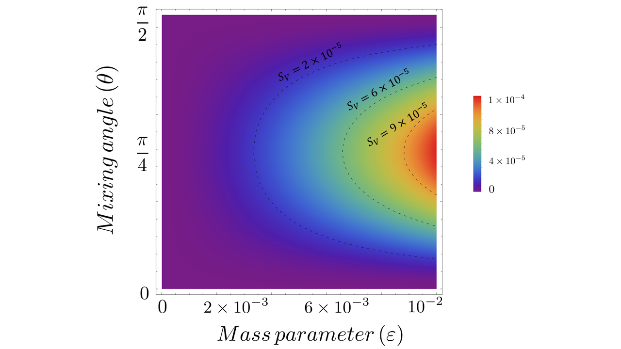
Figure 1: Behavior of von Neumann entanglement entropy $S_{V}$ as a function of $\varepsilon\in\left[0,10^{-2}\right]$ and $\theta\in\left[0,\frac{\pi}{2}\right]$. As explicitly shown by the level curves, $S_{V}$ monotonically decreases with decreasing $\varepsilon$.

As expected, in the limit of either $\varepsilon\to 0$ or $\theta\to 0$, we recover $S_{V}=0$, as it should correctly be, because in these cases the flavor vacuum reduces to the tensor product $|00\rangle_{1,2}=|0\rangle_{1}\otimes|0\rangle_{2}$. In Fig. 1 we report the behavior of von Neumann entropy as a function of both $\varepsilon$ and $\theta$. In order to better convey the dependence of $S_{V}$ on the mixing angle, it is also appropriate to exhibit how it varies by keeping $\varepsilon$ fixed. This is done in Fig. 2. In particular, we can notice that for arbitrary $\varepsilon$ the maximum of $S_{V}$ always occurs at the perfectly balanced mixing angle $\theta_{max}=\pi/4$. Increasing $\varepsilon$ only results in an upper shift in the magnitude of $S_{V}$, with an essentially invariant shape. The value of $\theta_{max}$ is exactly the one that could have been initially predicted, since $\pi/4$ corresponds to maximal mixing.

IV Conclusions

In this paper, we have explored some non-trivial features of the flavor vacuum in the case of mixing of two neutral scalar fields. A first preliminary analysis has shown that we cannot quantify entanglement by resorting to a direct comparison between $|00\rangle_{A,B}$ and the free thermal vacuum introduced in Thermo Field Dynamics, since the nature of the two states is not exactly the same. Note that this is consistent with the result found in Ref. bogoliubov in the context of neutrino mixing. A similar outcome has also been exhibited in Refs. prd , where it has been shown that the flavor vacuum for an accelerated observer is not strictly a thermal state, in contrast with the case of the standard Unruh effect. However, in spite of these differences, we have found that, in a proper limit, the flavor vacuum can be identified with the vacuum of TFD, with a temperature dependent on the mixing angle and the mass difference of the two mixed fields.

To further investigate the condensate structure of the flavor vacuum, we have restricted our attention to the mode $k=0$, for which the condensation density in $|00\rangle_{A,B}$ is maximal. In this setting, we have quantified von Neumann entropy for small values of the mass difference. The shape exhibited in Fig. 1 is the one derived from our analysis, and the picture of Fig. 2 shows that there is an angle in correspondence of which von Neumann entropy is maximal for a given value of the small mass difference. It is worth observing that such angle is precisely the one responsible for maximal mixing, namely $\theta_{max}=\pi/4$. Clearly, it would be interesting to go beyond the single-mode analysis and derive the full expression for the von Neumann entropy. However, we expect that the result will exhibit some ultraviolet divergence of the same kind as in Ref. Capozz , where the contribution of the flavor vacuum energy to the cosmological constant was shown to diverge only logarithmically, in contrast with the standard asymptotic behavior of free-field vacuum energy.

It is worth remarking that entanglement entropy and particle mixing have already been analyzed together in several papers in recent years entmix ; entmix2 , but only in the context of flavor transitions and for one-particle flavor states. In this respect, it is interesting to compare the field-theoretical approach to flavor entanglement developed in the present work with the exact methods for the quantification of entanglement introduced in the framework of quantum information and quantum optics of non-relativistic continuous variable systems (see for instance Refs. gaussian ; gaussian2 ; gaussian3 ; review and references therein). Such methods revolve around the transformation of the quadrature operators (namely, position and momentum) under a given operation, which in our case is the mixing transformation. Since at the level of these operators mixing acts merely as a rotation, we would not achieve the desired result, thus preventing us from reaching an accurate evaluation of the entanglement entropy of the flavor vacuum via the procedures adopted for quantum optical systems gaussian ; gaussian2 ; gaussian3 .

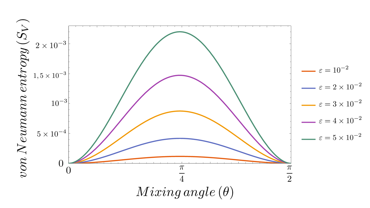
Figure 2: Behavior of von Neumann entanglement entropy $S_{V}$ as a function of $\theta\in\left[0,\frac{\pi}{2}\right]$ for different values of $\varepsilon$.

Finally, we emphasize that the present analysis may have several implications in a wide range of diversified contexts. For instance, once fully extended to non-inertial frames accCa ; accAl ; acc1 and, more generally, to gravity scenarios gravity ; gravity2 ; gravity3 ; gravity4 ; gravity5 ; gravity6 ; gravity7 ; gravity8 ; gravity9 ; gravity10 ; gravity11 , one could investigate how the information content of the flavor vacuum is degraded for increasing values of the acceleration/gravity. Note that a similar analysis has been carried out in Ref. fuentes1 for the case of the entanglement between two free modes of a scalar field as seen by an inertial observer detecting one of the modes and a uniformly accelerated observer detecting the other one. These and other aspects will be thoroughly investigated in future works.

Appendix A Thermo Field Dynamics

This Appendix is devoted to review the basics of Thermo-Field-Dynamics (TFD) tfd , which represents one of the approaches to QFT at finite temperature and density. The reason for this study lies in the fact the TFD and the formalism of mixing analyzed in Sec. II exhibit some non-trivial conceptual similarities, the most prominent one being the doubling of the degrees of freedom of the original system.

In order to introduce the TFD from a more quantitative point of view, let us consider the Hamiltonian of a free physical system written in the usual form

$$H=\sum_{k}\epsilon_{k}a^{\dagger}_{k}a_{k}\,.$$ (44)

We now define a completely identical fictitious system, which we name “tilde” system, sharing the same properties of the physical one. The former can then be written as

$$\tilde{H}=\sum_{k}\epsilon_{k}\tilde{a}^{\dagger}_{k}\tilde{a}_{k}\,.$$ (45)

The above relation allows us to establish a new set of “thermal” operators via the Bogoliubov transformations

$$a_{k}(\vartheta) = a_{k}\cosh\vartheta_{k}-\tilde{a}^{\dagger}_{k}\sinh\vartheta_{k}\,,$$ (46)

$$\tilde{a}_{k}(\vartheta) = \tilde{a}_{k}\cosh\vartheta_{k}-a^{\dagger}_{k}\sinh\vartheta_{k}\,,$$ (47)

with $\theta_{k}$ encoding the information about the original and thermal ladder operators. Notice that the transformations (46) and (47) leave the total Hamiltonian of the system $H_{tot}=H-\tilde{H}$ invariant, provided that the Hamiltonians (44) and (45) have the same spectrum.

The Bogoliubov transformation (46) and (47) can also be recast as

$$a_{k}(\vartheta) = e^{-iG}\,a_{k}\,e^{iG}\,,$$ (48)

$$\tilde{a}_{k}(\vartheta) = e^{-iG}\,\tilde{a}_{k}\,e^{iG}\,,$$ (49)

with

$$G=i\sum_{k}\vartheta_{k}\left(a_{k}^{\dagger}\tilde{a}^{\dagger}_{k}-\tilde{a}_{k}a_{k}\right)\,,$$ (50)

being the generator of the transformation, which is also a conserved quantity (namely $\left[G,H_{tot}\right]=0$) since the total Hamiltonian is conserved under its action. By means of $G$, we can now build a new vacuum state for the operators $a_{k}(\vartheta)$ and $\tilde{a}_{k}(\vartheta)$ defined as tfd

$$|0(\vartheta)\rangle=e^{-iG}|0\rangle\,,$$ (51)

where $|0\rangle$ is the vacuum associated with $a_{k}$ and $\tilde{a}_{k}$. If we explicitly act with the above operator on $|0\rangle$, we are left with

$$|0(\vartheta)\rangle=\prod_{k}\frac{e^{a^{\dagger}_{k}\tilde{a}^{\dagger}_{k}\tanh\vartheta_{k}}}{\cosh\vartheta_{k}}\,|0\rangle\,.$$ (52)

The above expression conveys the idea that the “theta” vacuum is actually a condensate of $a$- and $\tilde{a}$-particles, which somehow resembles the situation we have already encountered with mixing. However, in order to construct an effective comparison with the latter framework, we need to reformulate Eq. (52) as

$$|0(\vartheta)\rangle=e^{-\frac{\mathcal{K}}{2}}e^{\sum_{k}a_{k}^{\dagger}\tilde{a}^{\dagger}_{k}}|0\rangle=e^{-\frac{\tilde{\mathcal{K}}}{2}}e^{\sum_{k}a_{k}^{\dagger}\tilde{a}^{\dagger}_{k}}|0\rangle\,,$$ (53)

where

$$\mathcal{K}=-\sum_{k}\Bigl{(}a^{\dagger}_{k}a_{k}\ln\sinh^{2}\vartheta_{k}-a_{k}a^{\dagger}_{k}\ln\cosh^{2}\vartheta_{k}\Bigr{)}\,,$$ (54)

is called the entropy operator tfd , because its vacuum expectation value multiplied by $k_{B}$ yields precisely the entropy of the physical system. As a matter of fact, in order to make contact with a feasible physical picture and describe QFT for free fields at finite temperature, it is possible to prove that the arbitrary factors $\vartheta_{k}$ should satisfy the relation

$$\beta\,\omega_{k}=-\ln\tanh^{2}\vartheta_{k}\,,$$ (55)

with $\beta=(k_{B}T)^{-1}$ being the inverse of the emerging temperature $T$ of the thermal vacuum $|0(\vartheta)\rangle$ and $\omega_{k}=\epsilon_{k}-\mu$, where $\mu$ is the chemical potential. Remarkably, in the limit $\theta_{k}\rightarrow 0$ (i.e. for $T$ small enough), Eq. (52) reads

$$|0(\vartheta)\rangle\simeq\textbf{1}+\sum_{k}a^{\dagger}_{k}\tilde{a}^{\dagger}_{k}\vartheta_{k}|0\rangle\,.$$ (56)

As a final remark, we notice that the thermal vacuum (52), obtained by augmenting the physical Fock space by a fictitious “tilde” space, has the same condensate structure of the vacuum perceived by stationary (uniformly accelerating) observers outside black holes (in Minkowski spacetime). Of course, in that case the dual space can be interpreted in terms of the particle states on the hidden side of the horizon Israel ; unruh and the entanglement arises among modes across the horizon.

References

M. Blasone, F. Dell’Anno, S. De Siena, M. Di Mauro, and F. Illuminati, Phys. Rev. D 77, 096002 (2008).

M. Blasone, F. Dell’Anno, S. De Siena, and F. Illuminati, Europhys. Lett. 85, 50002 (2009).

S. Banerjee, A. K. Alok, and R. MacKenzie, Eur. Phys. J. Plus 131, 129 (2016).

V. A. S. V. Bittencourt, C. J. Villas Boas, and A. E. Bernardini, Europhys. Lett. 108, 50005 (2014).

Q. Fu and X. Chen, Eur. Phys. J. C 77, 775 (2017).

X. K. Song, Y. Huang, J. Ling, and M. H. Yung, Phys. Rev. A 98, 050302(R) (2018).

K. Dixit, J. Naikoo, S. Banerjee, and A. Kumar Alok, Eur. Phys. J. C 79, 96 (2019).

J. Naikoo, A. K. Alok, S. Banerjee, and S. U. Sankar, Phys. Rev. D 99 095001 (2019).

K. Dixit, J. Naikoo, B. Mukhopadhyay, and S. Banerjee, Phys. Rev. D 100 055021 (2019).

F. Ming, X. K. Song, J. Ling, L. Ye, and D. Wang, Eur. Phys. J. C 80, 275 (2020).

D. Wang, F. Ming, X. K. Song, L. Ye, and J. L. Chen, Eur. Phys. J. C 80, 800 (2020).

M. Blasone, F. Dell’Anno, S. De Siena, and F. Illuminati, Europhys. Lett. 106, 30002 (2014).

M. Blasone and G. Vitiello, Annals Phys.  244, 283 (1995).

S. M. Bilenky and B. Pontecorvo, Phys. Rep. 41, 225 (1978).

M. Blasone, M. V. Gargiulo, and G. Vitiello, Phys. Lett. B 761, 104 (2016).

A. Perelomov, Generalized Coherent States and Their Applications (Springer-Verlag, Berlin, 1986).

M. Blasone, P. Jizba, N. E. Mavromatos, and L. Smaldone, Phys. Rev. D 100, 045027 (2019).

M. Blasone, P. A. Henning, and G. Vitiello, Phys. Lett. B 451, 140 (1999).

M. Binger and C. R. Ji, Phys. Rev. D 60, 056005 (1999).

M. Blasone, A. Capolupo, O. Romei, and G. Vitiello, Phys. Rev. D 63, 125015 (2001).

M. Blasone, G. Lambiase and G. G. Luciano, J. Phys. Conf. Ser. 631, 012053 (2015); M. Blasone, G. Lambiase and G. G. Luciano, Phys. Rev. D 96, 025023 (2017); M. Blasone, G. Lambiase and G. G. Luciano, J. Phys. Conf. Ser. 880, 012043 (2017) M. Blasone, G. Lambiase and G. G. Luciano, J. Phys. Conf. Ser. 956, 012021 (2018).

A. Capolupo, G. Lambiase, and A. Quaranta, Phys. Rev. D 101, 095022 (2020).

A. Cabo Montes de Oca and N. G. Cabo Bizet, arXiv:2005.07758 [hep-ph] (2020).

H. Casini and M. Huerta, J. Phys. A: Math. Theor. 42, 504007 (2009).

J. Bardeen, L. N. Cooper, and J. R. Schrieffer, Phys. Rev.  108, 1175 (1957).

V. A. Miransky, Dynamical Symmetry Breaking in Quantum Field Theories (World Scientific, Singapore, 1993).

Y. Nambu, Phys. Rev.  117, 648 (1960); Y. Nambu and G. Jona-Lasinio, Phys. Rev. 122, 345 (1961).

J. Goldstone, Nuovo Cim.  19, 154 (1961), J. Goldstone, A. Salam, and S. Weinberg, Phys. Rev.  127, 965 (1962).

P. W. Higgs, Phys. Rev. Lett.  13, 508 (1964).

C. P. Burgess, Phys. Rept. 330, 193 (2000).

H. Casimir, Proc. K. Ned. Akad. Wet. 51, 793 (1948); H. Casimir and D. Polder, Phys. Rev. 73, 360 (1948).

K. A. Milton, The Casimir Effect: Physical Manifestations of Zero-Point Energy (World Scientific, Singapore, 2001).

M. Bordag, U. Mohideen, and V. M. Mostepanenko, Phys. Rep. 353, 1 (2001).

G. Lambiase, G. Scarpetta, and V. V. Nesterenko, Mod. Phys. Lett. A 16, 1983 (2001).

M. Blasone, G. G. Luciano, L. Petruzziello, and L. Smaldone, Phys. Lett. B 786, 278 (2018).

L. Mattioli, A. M. Frassino, and O. Panella, Phys. Rev. D 100, 116023 (2019).

M. Blasone, G. Lambiase, G. G. Luciano, L. Petruzziello, and F. Scardigli, Int. J. Mod. Phys. D 29, 2050011 (2020).

E. Calloni, L. di Fiore, G. Esposito, L. Milano, and L. Rosa, Int. J. Mod. Phys. A 17, 804 (2002).

F. Sorge, Class. Quant. Grav.  22, 5109 (2005).

S. A. Fulling, K. A. Milton, P. Parashar, A. Romeo, K. V. Shajesh, and J. Wagner, Phys. Rev. D 76, 025004 (2007).

G. Lambiase, A. Stabile, and An. Stabile, Phys. Rev. D 95, 084019 (2017)

M. Blasone, G. Lambiase, L. Petruzziello, and A. Stabile, Eur. Phys. J. C 78, 976 (2018).

L. Buoninfante, G. Lambiase, L. Petruzziello, and A. Stabile, Eur. Phys. J. C 79, 41 (2019).

S. W. Hawking, Nature 248, 30 (1974); Commun. Math. Phys.  43, 199 (1975).

W. G. Unruh, Phys. Rev. D 14, 870 (1976).

F. Scardigli, M. Blasone, G. Luciano and R. Casadio, Eur. Phys. J. C 78, 728 (2018); R. Casadio, P. Nicolini and R. da Rocha, Class. Quant. Grav. 35, 185001 (2018); F. Becattini and D. Rindori, Phys. Rev. D 99, 125011 (2019); G. Compère, J. Long and M. Riegler, JHEP 05, 053 (2019); S. Biermann, S. Erne, C. Gooding, J. Louko, J. Schmiedmayer, W. G. Unruh and S. Weinfurtner, Phys. Rev. D 102, 085006 (2020); J. Giné and G. G. Luciano, Eur. Phys. J. C 80, 1039 (2020).

H. Umezawa, Advanced Field Theory: Micro, Macro and Thermal Physics (American Institute of Physics, New York, 1993).

M. Blasone, P. Jizba, and G. G. Luciano, Annals Phys. 397, 213 (2018).

W. Israel, Phys. Lett. A 57, 107 (1976).

Y. Hashizume and M. Suzuki, Physica A 392, 3518 (2013).

M. Blasone, M. Di Mauro, and G. Vitiello, Phys. Lett. B 697, 238 (2011).

M. Blasone, A. Capolupo, S. Capozziello, S. Carloni, and G. Vitiello, Phys. Lett. A 323, 182 (2004).

G. Adesso, A. Serafini, and F. Illuminati, Phys. Rev. A 70, 022318 (2004).

G. Adesso and F. Illuminati, Phys. Rev. Lett. 95, 150503 (2005).

C. Weedbrook, S. Pirandola, R. García-Patrón, N. J. Cerf, T. C. Ralph, J. H. Shapiro, and S. Lloyd, Rev. Mod. Phys. 84, 621 (2012).

G. Adesso and F. Illuminati, J. Phys. A: Math. Theor. 40, 7821 (2007).

S. Capozziello and G. Lambiase, Eur. Phys. J. C 12, 343 (2000).

D. V. Ahluwalia, L. Labun, and G. Torrieri, Eur. Phys. J. A 52, 189 (2016).

M. Blasone, G. Lambiase, G. G. Luciano and L. Petruzziello, Phys. Rev. D 97, 105008 (2018); M. Blasone, G. Lambiase, G. G. Luciano and L. Petruzziello, Phys. Lett. B 800, 135083 (2020); M. Blasone, G. Lambiase, G. G. Luciano and L. Petruzziello, Eur. Phys. J. C 80, 130 (2020).

L. Stodolsky, Gen. Rel. Grav. 11, 391 (1979).

D. V. Ahluwalia and C. Burgard, Gen. Rel. Grav. 28, 1161 (1996).

C. Y. Cardall and G. M. Fuller, Phys. Rev. D 55, 7960 (1997).

S. Capozziello and G. Lambiase, Mod. Phys. Lett. A 14, 2193 (1999).

G. Lambiase, G. Papini, R. Punzi, and G. Scarpetta, Phys. Rev. D 71, 073011 (2005).

A. Geralico and O. Luongo, Phys. Lett. A 376, 1239 (2012).

L. Buoninfante, G. G. Luciano, L. Petruzziello, and L. Smaldone, Phys. Rev. D 101, 024016 (2020).

M. Blasone, G. Lambiase, G. G. Luciano, L. Petruzziello, and L. Smaldone, Class. Quant. Grav. 37, 155004 (2020).

A. Chatelain and M. C. Volpe, Phys. Lett. B 801, 135150 (2020); L. Petruzziello, Phys. Lett. B 809, 135784 (2020).

G. G. Luciano and L. Petruzziello, Int. J. Mod. Phys. D 29, 2043002 (2020).

P. Salucci, G. Esposito, G. Lambiase, E. Battista, M. Benetti, D. Bini, L. Boco, G. Sharma, V. Bozza and L. Buoninfante, et al. [arXiv:2011.09278 [gr-qc]].

I. Fuentes-Schuller and R. B. Mann, Phys. Rev. Lett.  95, 120404 (2005).