Conformal Floquet dynamics with a continuous drive protocol

Abstract

We study the properties of a conformal field theory (CFT) driven periodically with a continuous protocol characterized by a frequency $\omega_{D}$. Such a drive, in contrast to its discrete counterparts (such as square pulses or periodic kicks), does not admit exact analytical solution for the evolution operator $U$. In this work, we develop a Floquet perturbation theory which provides an analytic, albeit perturbative, result for $U$ that matches exact numerics in the large drive amplitude limit. We find that the drive yields the well-known heating (hyperbolic) and non-heating (elliptic) phases separated by transition lines (parabolic phase boundary). Using this and starting from a primary state of the CFT, we compute the return probability ($P_{n}$), equal ($C_{n}$) and unequal ($G_{n}$) time two-point primary correlators, energy density($E_{n}$), and the $m^{\rm th}$ Renyi entropy ($S_{n}^{m}$) after $n$ drive cycles. Our results show that below a crossover stroboscopic time scale $n_{c}$, $P_{n}$, $E_{n}$ and $G_{n}$ exhibits universal power law behavior as the transition is approached either from the heating or the non-heating phase; this crossover scale diverges at the transition. We also study the emergent spatial structure of $C_{n}$, $G_{n}$ and $E_{n}$ for the continuous protocol and find emergence of spatial divergences of $C_{n}$ and $G_{n}$ in both the heating and non-heating phases. We express our results for $S_{n}^{m}$ and $C_{n}$ in terms of conformal blocks and provide analytic expressions for these quantities in several limiting cases. Finally we relate our results to those obtained from exact numerics of a driven lattice model.

I Introduction

The study of driven quantum systems have attracted a lot of attention in recent years rev1 ; rev2 ; rev3 ; rev4 . The theoretical interest in this area stemmed from the fact that such systems provide access to a gamut of phenomena that have no analog in their equilibrium counterparts. Some of these phenomena, for periodically driven systems, include dynamical phase transitions heyl1 ; sen1 , dynamical freezing das1 ; pekker1 ; sen2 , realization of time crystals ach1 ; av1 , and the possibility of tuning ergodicity of the driven system with the drive frequency sen3 . Moreover, periodically driven systems can lead to novel steady states which has no counterpart in equilibrium quantum systems ach2 ; sen2 . The study of these phenomena has also received significant impetus from the possibility of realization of closed quantum systems using ultracold atom platforms; indeed, such platforms have recently been used to experimentally probe several non-equilibrium phenomena rev5 ; exp1 ; exp2 .

A large set properties of such periodically driven systems can be inferred from studying its Floquet Hamiltonin $H_{F}$ which is related to the evolution operator $U$ of the system via the relation $U(T,0)=\exp[-iH_{F}T/\hbar]$ rev3 . The computation of $H_{F}$ for a generic many-body system provides a significant challenge; indeed, an exact analytic computation of $H_{F}$ is generally possible for integrable models driven by discrete stepwise protocols (such a square pulse or kicks) rev3 . This has led to development of several perturbative schemes for computation of $H_{F}$; some of these include Magnus expansion rev3 , adiabatic-impulse approximation rev6 , the Hamilton flow method hamref , and the Floquet perturbation theory (FPT) ds1 ; tb1 . Out of these methods, the Floquet perturbation theory has the advantage of being easily applicable to a wide class of systems as well as being accurate over a large range of drive frequencies rg1 .

More recently, several theoretical studies concentrated on the effect of Floquet dynamics on conformal field theories cft1 ; cft2 ; cft3 ; cft4 ; cft5 ; cft6 . Usually driving a CFT is expected to generate an additional scale in the problem which drives the system away from its conformally invariant fixed point. However, it was recently realized that there is a class of models ssdpapers ; vidalpaper where drive protocols need not break the conformal symmetry cft1 . It is found that for CFTs with a sine square deformation (SSD) such dynamics can be initiated by a Hamiltonian whose holomorphic part is given by

$$H(t)=\frac{2\pi}{L}\left[f(t)L_{0}+\frac{1}{2}f_{1}(t)(L_{1}+L_{-1})\right],$$ (1)

where $L_{n}$ for each integer $n$ denotes a holomorphic generator of the Virasoro algebra,

$$[L_{m},L_{n}]=(m-n)L_{m-n}+\frac{c_{0}}{12}m(m^{2}-1)\delta_{m+n,0},$$ (2)

where $c_{0}$ denotes the central charge. These holomorphic generators are related to the stress tensor $T_{\mu\nu}$ of the CFT by

$$\begin{split}L_{0}&=\frac{L}{2\pi}\int_{0}^{L}dxT_{00}(w)\\ L_{\pm 1}&=\frac{L}{2\pi}\int_{0}^{L}dxe^{\pm 2\pi w/L}T_{00}(w)\end{split}$$ (3)

where $w=\tau+ix$, $x$ is the spatial coordinate and $\tau$ is the Euclidean time. The anti-holomorphic ones have a similar expression in terms of the complex conjugates.

It is well-known that the class of Hamiltonians given by Eq. 1 are valued in $su(1,1)$, giving rise to the evolution operator cft1

$$U(T,0)={\mathcal{T}}\ e^{-\tfrac{i}{\hbar}\int\limits_{0}^{T}H(t)dt}=\begin{pmatrix}a&b\\ c&d\end{pmatrix},$$ (4)

valued in the group $SU(1,1)$ with $ad-bc=1$. Using the isomorphism of $SU(1,1)$ and $SL(2,\mathbf{R})$ we shall also have occasion to write the evolution operator in imaginary time in the generic form

$$U(T=-i\tau,0)=\begin{pmatrix}\tilde{a}&\tilde{b}\\ \tilde{c}&\tilde{d}\end{pmatrix}\in SL(2,\mathbf{R}).$$ (5)

Its action on the complex plane $\mathbf{C}$ is given by the Möbius transformation

$$z\to z^{\prime}=\frac{\tilde{a}z+\tilde{b}}{\tilde{c}z+\tilde{d}},\quad z\in\mathbf{C}$$ (6)

where $\tilde{a},\tilde{b},\tilde{c},\tilde{d}\in\mathbf{R}$ and $\tilde{a}\tilde{d}-\tilde{b}\tilde{c}$=1.

The exact solution for $U(T,0)$ for Hamiltonians valued in $su(1,1)$ and driven by discrete protocols were discussed earlier for periodic kicks prapaper1 and square pulse protocols cft1 ; cft2 ; cft3 ; cft4 ; cft5 ; cft6 . It was found that such driven system could display two distinct phases depending on the drive parameters; these are termed as the heating (hyperbolic) and the non-heating (elliptic) phase and are found to be separated by a transition line (parabolic phase boundary) prapaper1 . The presence of these phases can be shown to be a direct consequence of non-compact nature of the SU(1,1) group. However, such studies have not been extended to continuous drive protocols where exact analytic results are not available comment1 ; in particular, the phase diagram of such a driven system for continuous drive protocols has not been studied so far.

It was noted in Ref. cft1, that the action of the evolution operator $U$ on a primary operator of the CFT can be understood, in the Heisenberg picture, in terms of a Möbius transformation of it’s coordinates leading to

$$U^{\dagger}(T,0)O(z,{\bar{z}})U(T,0)=\left(\frac{\partial z^{\prime}}{\partial z}\right)^{h}\left(\frac{\partial{\bar{z}^{\prime}}}{\partial{\bar{z}}}\right)^{{\bar{h}}}O(z^{\prime},{\bar{z}^{\prime}}),$$ (7)

where $z^{\prime}$ is defined in Eq. 6 and the bar designates anti-holomorphic variables throughout. Using this relation, and a straightforward mapping from cylindrical or strip geometries to the complex plane following standard prescription book1 , several results were obtained on the energy density, correlation function and entanglement entropy of the driven system cft1 ; cft2 ; cft3 ; cft4 ; cft5 ; cft6 . It was shown that in the heating phase, such a drive leads to emergent spatial structure of the energy density cft5 . Moreover, it was found that the time evolution of the entanglement entropy shows linear growth with $n$ (in the large $n$ or long-time limit) in the heating phase. In contrast, it shows an oscillatory behavior in the non-heating phase and a logarithmic growth on the parabolic phase boundary. All of these studies focussed on evolution starting from the CFT vacuum on a strip geometry cft1 ; cft2 ; cft3 ; cft4 ; cft5 ; cft6 ; the dynamics of the system starting from asymptotic states corresponding to primary operators of the theory, which necessitates computation of four-point correlation functions of the primary fields of the driven CFT, has not been studied so far.

In this work, we study dynamics of conformal field theories subjected to a continuous drive protocol. The protocol we use corresponds to the Hamiltonian given by Eq. 1 with $f_{1}(t)=1$ and

$$f(t)=f_{0}\cos(\omega_{D}t)+\delta f$$ (8)

where $f_{0}$ is the drive amplitude and $\delta f$ is a constant parameter. In this study we shall focus on the large drive amplitude regime which corresponds to $f_{0}\gg\delta f,1$. In this regime for $\omega_{D}\geq\delta f,1$, the FPT is expected to be accurate and we expect this to provide us with an analytic, albeit perturbative, understanding of the properties of the driven system.

The central results that we obtain from such a study are as follows. First, we chart out the phase diagram of the driven system as a function of $\delta f$ and $\omega_{D}$ using exact numerics. Our results show re-entrant heating and non-heating phases separated by a parabolic phase boundaries as a function of $\delta f$ and $T$. Second, we provide analytic expressions of the evolution operator $U(T,0)$ using FPT. The phase diagram obtained from the perturbative result provides a near-exact match with its exact numerical counterpart over a wide range of frequencies. Our perturbative results indicate the existence of a parameter $\alpha$, given within first order FPT by (where we have put $\hbar=1$)

$$\alpha = \sum_{n=-\infty}^{\infty}J_{n}\left(\frac{2f_{0}\pi}{L\omega_{D}}\right)\frac{T}{(n\pi+\pi\delta fT/L)},$$ (9)

which indicates proximity of the system to the phase boundary. The system stays in the non-heating phase for $\alpha^{2}<1$ and heating phase for $\alpha^{2}>1$; the phase boundary between these two phases is given by $\alpha=\pm 1$. We also use the first order FPT results to explain the re-entrant transitions between the heating and the non-heating phases in the phase diagram. Third, we use the obtained expressions for $U$ within FPT, to obtain analytic expressions for energy density, equal and unequal time two-point correlation functions, entanglement entropy, and return probability of generic sine-square deformed CFT starting from a primary state. Our results expresses these quantities in terms of $\alpha$ and allows us to characterize their behavior near the transition from the heating phase. For example, we find that the return probability of any primary state after $n$ drive cycles shows an universal behavior below a crossover time $n_{c}$ both in the heating and the non-heating phases near the transition line; for $n>n_{c}$, the probability decays exponentially for the heating phase and remains an oscillatory function in the non-heating phase. We provide analytic estimate of $n_{c}$ as a function of $\alpha$. Fourth, we discuss the nature of the emergent spatial structure of the energy density and the correlation function of primary operators for the drive protocol. We analytically show that the energy density of any primary state in the heating phase displays peaks which shifts from $L/4$ and $3L/4$ to $L/2$ as one moves from deep inside the heating phase to the transition line. For unequal-time correlation function starting from the CFT vacuum, we find a line of such peaks both in the heating and the non-heating phases; the position of these peaks can be analytically found within first order FPT. Finally, we provide expressions of the equal-time correlation function $C_{n}$ and half-chain $m^{\rm th}$ Renyi entropy $S_{n}^{m}$ of the driven CFT after $n$ drive cycles starting from an initial primary state in terms of conformal blocks ${\mathcal{V}}_{p}$. In general, these blocks do not have analytical expression for arbitrary CFTs; here, we provide their analytical forms in several asymptotic limits. We discuss the applicability of these limits to the driven CFT and discuss the properties of $C_{n}$ and $S_{n}^{m}$ in these asymptotic regimes. Finally, we relate some of our results to those obtained by exact numerical study of the SSD model on a 1D lattice ssdpapers ; vidalpaper .

The plan of the rest of the paper is as follows. In Sec. II, we derive expressions of $U$ and provide the phase diagram for our drive protocol. This is followed by Sec. III where we compute energy density, correlation functions and return probabilities starting from a primary state. Next, in Sec. IV, we relate our results to those obtained from numerical study of driven SSD Hamiltonian on a 1D lattice. Finally, we discuss our main results and conclude in Sec. V. Some details of the perturbative FPT calculations and representation independent derivation of the Mobius transformation are presented in the Appendices.

II Phase Diagram

To find $U(T,0)$ corresponding to the Hamiltonian given by Eq. 1 with $f(t)$ given by Eq. 8, we first note that the holomorphic generators (Eq. 2) for $n=-1,0,1$ form an $su(1,1)$ subalgebra

$$[L_{0},L_{-1}]=L_{-1},\quad[L_{0},L_{1}]=-L_{1},\quad[L_{-1},L_{1}]=-2L_{0}.$$ (10)

A representation of this algebra is furnished in terms of the Pauli matrices as

$$L_{0}=\tfrac{1}{2}\sigma_{z},\quad L_{\mp 1}=\pm\sigma^{\mp},\quad\sigma^{\pm}=\frac{1}{2}(\sigma_{x}\pm i\sigma_{y}),$$ (11)

where $\sigma_{\alpha}$ for $\alpha=x,y,z$ are standard Pauli matrices. In this representation (Eq. 11), the holomorphic part of the Hamiltonian $H(t)$ becomes

$$H(t) = \frac{\pi}{L}\left(f(t)\sigma_{z}-i\sigma_{y}\right)\$$ (12)

which corresponds to a Zeeman Hamiltonian of a single spin-half particle with a time dependent magnetic field along $\hat{z}$ and an imaginary constant magnetic field along $y$. The latter feature is a consequence of the SU(1,1) group structure and is crucial in realization of the heating and the non-heating phases prapaper1 . The expression for $U(T,0)$ corresponding to Eq. 12 can be found exactly for periodic kicks prapaper1 and square-pulse cft1 protocols.

In contrast, for the continuous protocol given by Eq. 8, an exact analytic expression for $U(T,0)$ does not exist. However, the numerical result for $U$ can be obtained in a straightforward manner. Such a numerics is carried out by dividing the time period $T$ into $N$ Trotter steps with width $\delta t_{i}\sim T/N$. The maximal allowed width of each of these steps depend on system energy scale and the drive frequency; they are chosen so that $H$ does not vary appreciably within any step. This allows one to write $U\simeq\prod_{i=1,N}U_{i}$, where $U_{j}=U(t_{j-1}+\delta t_{j},t_{j-1})=\exp[-i\int_{t_{j-1}}^{t_{j-1}+\delta t_{j}}dtH(t)/\hbar]$. This procedure leads to $U(T,0)=\exp[-iH_{F}T/\hbar]$; we find numerically that the Floquet Hamiltonian is

$$H_{F} = p(T)\sigma_{z}+iq(T)\sigma_{y}$$ (13)

We note that $\sigma_{x}$ does not appear in $H_{F}$. The condition for the different phases are thus obtained by prapaper1 $|{\rm Tr}U(T,0)|>2$ (heating phase), $<2$ (non-heating phase), and $=2$ (phase boundary). The exact numerical phase diagram obtained from this procedure is shown in the left panel of Fig. 1. We find several re-entrant transitions between the heating and the non-heating phases leading to multiple lobes whose boundary correspond to the transition lines. We note that the transition between these phases can be induced by tuning either $\delta f$ or $\omega_{D}$. In particular, we note that large $\hbar\omega_{D}\gg\delta f,1$, the phase transition between the heating and non-heating phase occurs at $\delta f=1$.

The absence of $\sigma_{x}$ in $H_{F}$ can be shown to be the consequence of an emergent dynamic symmetry of the evolution operator at stroboscopic times which follows from the periodicity of $H(t)$. To see this we note that since $H(t)=H(T-t)$, one has $U_{j}=U_{N-j+1}$ for all $j$ in the Trotter product. Further, we note for any of these Trotter steps, one has $\sigma_{x}U_{j}\sigma_{x}=U_{j}^{-1}$. Thus one can write

$$\sigma_{x}U(T,0)\sigma_{x} = \sigma_{x}\left(\prod_{j=1,N}U_{j}\right)\sigma_{x}$$

$$= \prod_{j=1,N}U^{-1}_{j}=\left(\prod_{j=1,N}U_{j}\right)^{-1}=U^{-1}(T,0)$$

where we have used the relation $U_{j}^{-1}=U_{N-1+j}^{-1}$. Eq. II clearly implies that if $U=\exp[-iH_{F}T]$ then $\sigma_{x}H_{F}\sigma_{x}=-H_{F}$. This forbids presence of terms $\sim\sigma_{x}$ in $H_{F}$. It is to be noted that this symmetry is absent for $t\neq nT$ where $n$ is an integer.

Next, we develop an perturbative analytic expression of $U$ in the limit when $f_{0}$ is the largest scale in the problem. Here the diagonal term in $H(t)$ is treated exactly and the effect of the off-diagonal term is taken into account within standard time-dependent perturbation theory tb1 . In this scheme, the first term for $U$ and $H_{F}$ is given by

$$U_{0}(t,0) = e^{-i(\pi/L)(f_{0}\sin\omega_{D}t/\omega_{D}+\delta ft)\sigma_{z}}$$

$$H_{F}^{(0)} = s\sigma_{z}/T$$ (15)

where $s=\arccos[\cos(\delta fT\pi/L)]$. We note that $H_{F}^{(0)}$ retain the periodic structure of $U_{0}$.

To obtain the first order correction to $U(T,0)$, we use the standard result tb1

$$U_{1}(T,0)=U_{0}(T,0)(I-U^{\prime}_{1}(T,0))$$ (16)

where $I$ denotes the $2\times 2$ identity matrix and $U^{\prime}_{1}$ denotes the first-order correction to $U$ in the interaction picture given by

$$U^{\prime}_{1}(T,0) = -i\int_{0}^{T}dtU_{0}^{\dagger}(t,0)H_{1}U_{0}(t,0)$$ (17)

where $H_{1}=-\frac{\pi}{L}i\sigma_{y}$ is the perturbative term of the Hamiltonian. A simple calculation detailed in App. A yields

$$U^{\prime}_{1}(T,0) = i\alpha e^{is}\sin(s)\sigma_{y}$$

$$U_{1}(T,0) = \left(\begin{array}[]{cc}e^{-is}&-i\alpha\sin s\\ i\alpha\sin s&e^{is}\end{array}\right)$$ (20)

where $\alpha$ is given by Eq. 9. We note that $U_{1}(T,0)$ is not unitary; this is a well-known issue with perturbation theory for $U$. In what follows we unitarize $U_{1}(T,0)$ as follows. We note that this can be done by first writing $(I-U^{\prime}_{1}(T,0))\simeq\exp[-iH^{\prime}_{F}T]$, where the matrix $H^{\prime}_{F}=(i/T)U^{\prime}_{1}$. The evolution operator is then given by $U_{0}(T,0)\exp[-iH^{\prime}_{F}T]$ which is unitary. However, in the present case, we find that evolution operator obtained by this method retains terms $\sim\sigma_{x}$. This is clearly inconsistent with the dynamic symmetry discussed in Eq. II. Thus we chose to unitarize $U_{1}(T,0)$ directly since it does not have any term $\sigma_{x}$. These two alternative routes to obtaining $H_{F}$ coincides with each other in the large $\omega_{D}$ limit, where $s\to 0$.

The unitarization of $U_{1}(T,0)$ given by Eq. 20 can be achieved by writing

$$U_{1}(T,0) = \exp[-i\theta(\sigma_{z}n_{z}+\sigma_{y}n_{y})],\quad\theta=s\sqrt{1-\alpha^{2}}$$

$$n_{z} = \frac{1}{\sqrt{1-\alpha^{2}}},\quad n_{y}=\frac{i\alpha}{\sqrt{1-\alpha^{2}}}$$ (21)

Comparing Eqs. 13 and 21, we find that the first order FPT result provides approximate analytic expressions for $p(T)$ and $q(T)$ given by

$$q/p \simeq \alpha,\quad p\simeq s/T$$ (22)

In what follows we shall use Eq. 22 to compare between exact numeric and approximate analytic results.

The evolution operator obtained in Eq. 21 indicates several interesting features. First, we find that $n_{y}$ is imaginary; this is a direct consequence of the SU(1,1) group structure. Second, we note that ${\rm Tr}[U_{1}(T,0)]=2\cos(\theta)$; thus the condition $|{\rm Tr}[U_{1}(T,0)]|>(<)2$ for realization of heating (non-heating) phases translates to $\theta$ being imaginary(real). This happens when $\alpha^{2}>(<)1$ which leads to our identification of $\alpha$ as the parameter whose value determines the phase the system. Third, the parabolic phase boundary between these two phases is given by $|{\rm Tr}[U_{1}(T,0)]|=2$ which leads to $\theta=0$. This is realized for $\alpha=\pm 1$ on the boundary between the heating and non-heating phases. From the expression of $\alpha$ in Eq. 9, we find that for $\omega_{D}\gg f_{0}$, the condition $\alpha=1$ is satisfied for $\delta f=1$. This can be verified directly from the exact phase diagram in the left panel of Fig. 1. Fourth, the re-entrance of the heating and non-heating phases as a function of $\delta f$ shown in the right panel of Fig. 1 displaying the phase diagram obtained from first order FPT, can be easily explained by periodic nature of $|\cos(\theta)|$ since the phases must repeat for $\theta\to\theta+\pi$. We note the two phase boundaries in each of the lobes of this phase diagram correspond to $\alpha=1$ (lower branch of the lobes) and $\alpha=-1$ (upper branch of the lobes). The center of these lobes correspond to $\alpha\to\infty$ which occurs along the lines $\delta f/\omega_{D}=n_{0}/2$ for $n_{0}\in Z$. This can be directly seen from Eq. 9 where the term in the sum corresponding to $n=n_{0}$ diverges in this limit. Finally, a comparison between the left and the right panels of Fig. 1 shows that the two phase diagrams match qualitatively for $\hbar\omega_{D}/(\pi/L)>1$. This allows us to justify the use of the analytical method for a qualitative understanding of the dynamics within first order FPT. A computation of the second-order results of FPT is carried out in App. A; we find that it retains all features of the first order theory and provides a near-identical phase diagram. In App. B, we chart out a representation independent derivation of the first order perturbation results in the high frequency limit which matches the results obtained here using the SU(1,1) representation of the Virasoro generators.

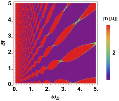
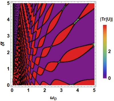
Figure 1: (Color online) Left Panel: Plot of the phase diagram, obtained from $|{\rm Tr}U(T,0)|$ plotted as a function of the amplitude $\delta f$ and frequency $\omega_{D}$ as obtained from exact numerics. The red regions indicate heating phases while the violet ones show the non-heating phases. The re-entrant transition between these phases are shown by black lines indicating parabolic transition lines. Right Panel: Similar phase diagram obtained from first order FPT. For both plots, we have set $\pi/L$ to unity and set $f_{0}=10$.

Before ending this section , we obtain the elements of $U^{n}=U(nT,0)$ (where $n\in Z$ is an integer). Using Eqs. 4 and 13, we find the elements of $U^{j}$ for any integer $j$ obtained using exact numerics in the non-heating phase (where $p>q$) to be

$$a_{j} = \cos(\sqrt{p^{2}-q^{2}}jT)-i\frac{p}{\sqrt{p^{2}-q^{2}}}\sin(\sqrt{p^{2}-q^{2}}jT)$$

$$b_{j} = \frac{iq}{\sqrt{p^{2}-q^{2}}}\sin(\sqrt{p^{2}-q^{2}}jT)$$ (23)

where $d_{j}=a_{j}^{\ast}$ and $c_{j}=b_{j}^{\ast}$. For the heating phase, for which $p<q$, one obtains

$$a^{\prime}_{j} = \cosh(\sqrt{q^{2}-p^{2}}jT)-i\frac{p}{\sqrt{q^{2}-p^{2}}}\sinh(\sqrt{q^{2}-p^{2}}jT)$$

$$b^{\prime}_{j} = \frac{iq}{\sqrt{q^{2}-p^{2}}}\sinh(\sqrt{q^{2}-p^{2}}jT)$$ (24)

For the transition line where $p=q$, a careful evaluation of the limit shows

$$a"_{j} = 1-ipjT,\quad b"_{j}=-ipjT$$ (25)

The corresponding analytic, first order FPT, expressions of elements of $U(jT,0)$ in terms of $\alpha$ and $s$ can be directly read off from these equations by using the correspondence expressed in Eq. 22. For example for the transition line, the first order FPT result is $a"_{j}=1-ijs$ and $b"_{j}=-ijs$. Also, the corresponding elements $\tilde{a}_{j}$, $\tilde{b}_{j}$, $\tilde{c}_{j}$ and $\tilde{d}_{j}$ of the evolution operator in Euclidean time can be obtained for each of these phase from Eqs. 23, 24, and 25 via standard analytic continuation $T\to-i\tau$. We shall use these expressions in the next section computation of return probability, energy density, correlation functions and the entanglement entropy.

III Results for driven CFT

It was pointed out in Ref. cft1, that the operation of the evolution operator $U$ on any primary operator of the CFT can be understood in terms of a Möbius transformation of its coordinates and is therefore given by Eq. 7. This is further discussed in App. B. In this section, we shall use this result to study the properties of the driven CFT with a cylindrical geometry which corresponds to periodic boundary condition of a driven 1D chain of length $L$. In our setup, the coordinate of the cylinder is given by $w=\tau+ix$, where $x$ is the spatial coordinate and $\tau$ is the Euclidean time; we use $w=(L/(2\pi))\ln z$ for mapping such a cylinder to the complex plane. Thus for any primary operator ${\mathcal{O}}(w,\bar{w})$ on the cylinder, we can write book1 ; cft1

$$U^{n\dagger}{\mathcal{O}}(w,\bar{w})U^{n} = \left(\frac{\partial w}{\partial z}\right)^{-h}\left(\frac{\partial z_{n}}{\partial z}\right)^{h}\left(\frac{\partial{\bar{w}}}{\partial{\bar{z}}}\right)^{-{\bar{h}}}$$ (26)

$$\times\left(\frac{\partial{\bar{z}}_{n}}{\partial{\bar{z}}}\right)^{{\bar{h}}}{\mathcal{O}}(z_{n},{\bar{z}}_{n})$$

where $z_{n}$ is the transformed coordinates given by Eq. 6 and $\tilde{a}_{n}$, $\tilde{b}_{n}$, $\tilde{c}_{n}$, and $\tilde{d}_{n}$ are the elements of $U^{n}$ in Euclidean time which can be obtained from analytic continuation of $T\to-i\tau$ in Eqs. 23, 24 and 25. In all computations, we shall work in Euclidean time and carry out the analytic continuation to real time using $\tau=iT$ at the end of the calculation.

Apart from the primary operators we shall also use transformation properties of the stress tensor. The holomorphic part of the stress tensor denoted by $T(w)$ transforms, under a general coordinate transformation, as $T(w)\to T^{\prime}(w^{\prime})=(\partial w^{\prime}/\partial w)^{-2}(T(w)+S_{w^{\prime},w})$, where $S$ is Schwarzian given by

$$S_{w^{\prime},w} = \frac{c_{0}}{12}\left[\left(\frac{\partial^{3}w^{\prime}}{\partial w^{3}}\right)\left(\frac{\partial w^{\prime}}{\partial w}\right)^{-1}\right.$$ (27)

$$\left.-\frac{3}{2}\left(\left(\frac{\partial^{2}w^{\prime}}{\partial w^{2}}\right)\left(\frac{\partial w^{\prime}}{\partial w}\right)^{-1}\right)^{2}\right]$$

Here we note that $S_{z_{n},z}=0$ since $S$ vanishes for any Möbius transformation and $S_{z,w}=c_{0}/(24z^{2})$ for transformation from a cylinder to the complex plane. The transformation for the antiholomorphic part of the stress tensor can be obtained in the similar manner by replacing $(w^{\prime},w)\to({\bar{w}}^{\prime},\bar{w})$.

In what follows, we shall use these general results to obtain the stroboscopic time ($n$) dependence of the return probability, energy density, equal and unequal time correlation functions, and the entanglement entropy of the driven CFT. The initial state for this purpose is chosen to be an asymptotic in-state of the CFT denoted by

$$|h,\bar{h}\rangle = \lim_{w,{\bar{w}}\to-\infty}\phi(w,\bar{w})|0\rangle$$ (28)

where $|0\rangle$ denotes the CFT vacuum, $\phi$ is a primary field with dimension $(h,\bar{h})$ and we note $w,{\bar{w}}\to-\infty$ corresponds to $\tau\to-\infty$ which in turn implies $z,{\bar{z}}\to 0$ on the complex plane. This defines for us a primary state. The corresponding out-states are given by

$$\langle h,\bar{h}| = \langle 0|\lim_{w,{\bar{w}}\to\infty}\phi(w,\bar{w})$$ (29)

which corresponds to $\tau\to\infty$ and hence $z,\bar{z}\to\infty$ on the complex plane.

The reason for choosing these primary states are as follows. First, we note that since $L_{0}$ and $L_{\pm 1}$ annihilates the CFT vacuum, the vacuum state does not evolve. This renders all equal time correlation functions of primary operators, entanglement entropy and energy density to be fixed at their equilibrium values under action of $U$; only the unequal-time correlation function shows non-trivial dynamics. This feature of driven CFT usually compels one to work with the strip geometry cft1 ; cft4 or use different Möbius transformation cft5 where one can obtain non-trivial time evolution starting from the ground state. Here we use an alternative approach by using the cylindrical geometry but starting from the primary states of the CFT ($|h,\bar{h}\rangle$) as initial states; these are the simplest states of the model which have non-trivial dynamics under action of $U$.

III.1 Return probability and energy density

The return probability amplitude $A_{n}$ after $n$ cycles of the drive is given by

$$A_{n} = \frac{\langle h,\bar{h}|U(nT,0)|h,\bar{h}\rangle}{\langle h,\bar{h}|h,\bar{h}\rangle|}$$ (30)

where the denominator corresponds to the normalization of the asymptotic states. To this end, we first look at the contribution of the holomorphic part of the return probability amplitude given by

$$A_{n}^{\rm hol} = \frac{\lim_{w_{1}\to 0,w_{2}\to\infty}\langle 0|\phi(w_{2})U(nT,0)\phi(w_{1})|0\rangle}{\lim_{w_{1}\to 0,w_{2}\to\infty}\langle 0|\phi(w_{2})\phi(w_{1})|0\rangle}=\frac{\mathcal{N}}{\mathcal{D}}$$

To compute $A_{n}^{\rm hol}$, we take $w_{i}=\tau_{i}+ix_{i}$ for $i=1,2$ and consider the limits $\tau_{1}\to-\infty$ and $\tau_{2}\to\infty$ at the end of the calculation. Using the fact that $\langle 0|U^{\dagger}=\langle 0|$, we can rewrite as ${\mathcal{N}}=\langle 0|U^{n\dagger}\phi(w_{2},\bar{w}_{2})U^{n}\phi(w_{1},{\bar{w}}_{1})|0\rangle$. We then use Eq. 26 to obtain

$${\mathcal{N}} = \lim_{z_{2}\to\infty,z_{1}\to 0}\left(\frac{2\pi}{L}\right)^{2h}\left(\frac{z_{1}z_{2}}{(\tilde{c}_{n}z_{2}+\tilde{d}_{n})^{2}(z_{n2}-z_{1})^{2}}\right)^{h}$$

$${\mathcal{D}} = \lim_{z_{2}\to\infty,z_{1}\to 0}\left(\frac{2\pi}{L}\right)^{2h}\left(\frac{z_{1}z_{2}}{(z_{2}-z_{1})^{2}}\right)^{h}$$ (32)

where $z_{n2}=(\tilde{a}_{n}z_{2}+\tilde{b}_{n})/(\tilde{c}_{n}z_{2}+\tilde{d}_{n})$ is the transformed coordinate, $\tilde{a}_{n}$, $\tilde{b}_{n}$, $\tilde{c}_{n}$ and $\tilde{d}_{n}$ are obtained from Eqs. 23, 24 ,25 after analytic continuation $T=-i\tau$ and we have used $\partial w/\partial z=L/(2\pi z)$ and $\partial z_{n2}/\partial z=(\tilde{c}_{n}z_{2}+\tilde{d}_{n})^{-2}$. After a careful evaluation of the limits, we finally obtain $A_{n}^{\rm hol}=\tilde{a}_{n}^{-2h}$. A similar computation shows the contribution from the anti-holomorphic part to be $A_{n}^{{\rm ant-hol}}=\tilde{a}_{n}^{-2\bar{h}}$. Thus one obtains the return probability $P_{n}$, after analytic continuation to real time, to be

$$P_{n} = |A_{n}^{\rm hol}A_{n}^{{\rm ant-hol}}|^{2}=|a_{n}|^{-4(h+\bar{h})}$$ (33)

The exact numerical value of $P_{n}$ can thus be obtained by using Eqs. 23, 24, 25. Here and for all quantities in the rest of this section, we shall provide expressions for the prediction of FPT; the numerical result in terms of $p$ and $q$ can be directly read from these expressions by using Eq. 22(i.e. with the mapping $\alpha\to p/q$ and $s\to pT$). This procedure yields

$$P_{n} = \left(\frac{\alpha^{2}(1+\cosh n\theta)-2}{2(\alpha^{2}-1)}\right)^{-2(h+\bar{h})},\,{\rm heating}$$ (34)

$$= \left(\frac{2-\alpha^{2}(1+\cos n\theta)}{2(1-\alpha^{2})}\right)^{-2(h+\bar{h})},\,{\rm non-heating}$$

$$= (1+n^{2}s^{2})^{-2(h+\bar{h})},\quad{\rm transition\,line}$$

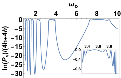
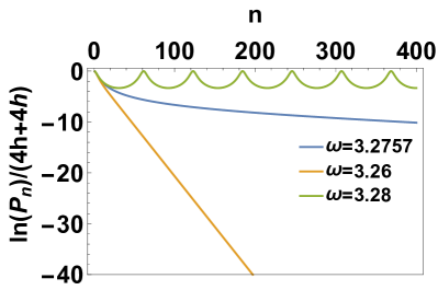
Figure 2: (Color online) Left Panel: Plot of $\ln P_{n}/(4(h+\bar{h}))$ as a function of frequency $\omega_{D}$ for after $n=50$ cycles of the drive. The inset shows the variation of $\ln P_{n}$ with $\omega_{D}$ in the non-heating phase. Right Panel: Plot of $\ln P_{n}/(4(h+\bar{h}))$ as a function of $n$ for three representative drive frequencies corresponding to the heating ($\omega_{D}=3.26$ orange line) and non-heating phases ($\omega_{D}=3.28$, green line) and the transition line ($\omega_{D}\simeq 3.2767$, blue line). In all plots $\pi/L$ has been set to unity, $f_{0}=10$ and $\delta f=0.5$. See text for details.

The behavior of $\ln P_{n}$ is shown in the left panel of Fig. 2 as a function of drive frequency after $n=50$ cycles of the drive and for $\delta f=0.5$. We find that $\ln P_{n}$ shows dips at large $n$ in the heating phases; in contrast, it shows oscillatory behavior near the transition in the non-heating phase as can be seen from the inset of the left panel of Fig. 2. We also note that the return probability shows an exponential decay for large $n$ in the heating phase and an oscillatory behavior in the non-heating phase according to standard expectation. On the transition line, it shows a power law decay $\sim n^{-2(h+\bar{h})}$ for large $n$. These qualitatively different behaviors of $P_{n}$ can be clearly seen in the right panel of Fig. 2 where $\ln P_{n}$ is plotted as a function of $n$ for three values of drive frequencies corresponding to three different phases. Here we also note that near the phase transition line, in either phase, the behavior of $P_{n}$ is identical to that on the critical line below a crossover timescale $n\leq n_{c}$. This is most easily seen by expanding the $\cosh(n\theta)$ term in powers of $n\theta$ in Eq. 34. This procedure yields, in the heating phase,

$$\ln P_{n}\simeq-2(h+\bar{h})\ln\left[1+(\alpha sn)^{2}+(\alpha sn)^{4}\frac{\alpha^{2}-1}{3\alpha^{2}}+...\right]$$

$$n_{c}\simeq\sqrt{3}/(s\sqrt{\alpha^{2}-1})$$ (35)

where the ellipsis denote terms higher order in $n$. We note that $n_{c}$ here is estimated as $n$ for which the contribution of the term $\sim n^{4}$ becomes equal to the leading term $\sim n^{2}$. We find that $n_{c}$ diverges at the transition as $1/\sqrt{\alpha^{2}-1}$ as one approach the transition from the heating phase; it can also be made large by tuning either the drive frequency or amplitude since $s\sim\delta fT$. For $n\ll n_{c}$, the behavior $P_{n}$ is identical to that on the transition line. A similar result can be obtained if the transition line is approached from the non-heating phase. Thus we find that characteristic behavior the return probability on the transition line can be observed upon approaching the line below a crossover timescale $n_{c}$ which diverges at the transition; $P_{n}$ has a universal dependence on $s$ for $n\ll n_{c}$. This behavior is shown in Fig. 3 in the high drive frequency regime $(\hbar\omega_{D})/(\pi/L)=100$ where $\delta f=1$ gives the position of the transition line. We clearly see that $\ln P_{n}$ remains indistinguishable for $n\leq n_{c}\simeq 50$. The divergence of $n_{c}$ at the transition line is shown in the right panel of Fig. 3.

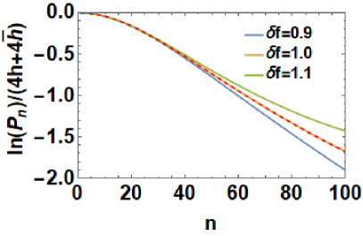
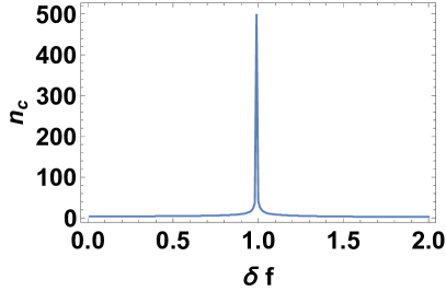
Figure 3: (Color online) Left Panel: Plot of $\ln P_{n}/(4(h+\bar{h}))$ as a function of frequency $n$ for $\delta f=1.1$ (non-heating phase, green line), $1$ (transition line, yellow line) and $0.9$ (heating phase, blue line) with $\omega_{D}=100$. The red dashed line is a plot of $-\ln(1+s^{2}n^{2})$. Right panel: Plot of $n_{c}$ as a function of $\delta f$ for $\omega_{D}=100$ showing a sharp peak at the transition. For all plots $\pi/L$ has been set to unity, and $f_{0}=10$. See text for details.

Next, we study the behavior of the energy density of the driven system given by

$$E_{n} = \frac{\langle h,\bar{h}|U^{\dagger n}(T(w)+{\bar{T}}(\bar{w}))U_{n}|h,\bar{h}\rangle}{\langle h,\bar{h}|h,\bar{h}\rangle}$$ (36)

To evaluate this, we first consider the holomorphic contribution to the energy density. To this end, we first move from the cylinder to the complex plane so that one can write

$$T(w) = \left(\frac{2\pi z}{L}\right)^{2}T(z)+c_{1}$$ (37)

where the constant term $c_{1}=(2\pi/L)^{2}c_{0}/24$ comes from the Schwarzian given by Eq. 27 and $c_{0}$ denotes the central charge. In what follows we shall ignore this term since it does not change upon driving the system. Using this and Eqs. 26 we find

$$\langle h|U^{\dagger n}T(w)U^{n}|h\rangle=\lim_{z_{2}\to\infty,z_{1}\to 0}\left(\frac{2\pi}{L}\right)^{2(1+h)}z_{1}^{h}z_{2}^{h}z^{2}$$

$$\quad\times(\tilde{c}_{n}z+\tilde{d}_{n})^{-4}\langle 0|\phi(z_{2})T(z_{n})\phi(z_{1})|0\rangle$$ (38)

where we have used $w=ix$ so that $z=\exp[2\pi ix/L]$ and $w_{i}=\tau_{i}$ for $i=1,2$ with $\tau_{1}\to-\infty$, $\tau_{2}\to\infty$ leading to the limits $z_{2}\to\infty$ and $z_{1}\to 0$.

Eq. 38 reduces the computation of the energy density to that of computation of $\langle\phi T\phi\rangle$ correlator in the CFT vacuum state. This can be done in a straightforward manner using standard identity bpz1 and yields

$$\langle 0|\phi(z_{2})T(z_{n})\phi(z_{1})|0\rangle = h\left[(z_{n}-z_{2})^{-2}(z_{2}-z_{1})^{-2h}+(z_{n}-z_{1})^{-2}(z_{2}-z_{1})^{-2h}\right.$$ (39)

$$\left.-2(z_{n}-z_{2})^{-1}(z_{2}-z_{1})^{-(2h+1)}-2(z_{n}-z_{1})^{-1}(z_{2}-z_{1})^{-(2h+1)}\right]$$

We substitute Eq. 39 in Eq. 38 and find that in the limit $z_{2}\to\infty$ only the second term in the right side of Eq.  39 contribute. Taking the $z_{1}\to 0$ limit, we finally obtain the holomorphic contribution to the energy density to be

$$E_{n}^{\rm hol} = \left(\frac{2\pi}{L}\right)^{2}\frac{h}{(R_{1n}(x)R_{2n}(x))^{2}}$$ (40)

$$R_{1(2)n}(x) = [\tilde{a}_{n}(\tilde{c}_{n})e^{\pi ix/L}+\tilde{b}_{n}(\tilde{d}_{n})e^{-\pi ix/L}]$$ (41)

The antiholomorphic contribution can be simply read off from this to be $E_{n}^{\rm hol}(x)=E_{n}^{\rm ant-hol}(-x)$. Thus the total energy density which is the sum of the holomorphic and anti-holomorphic parts are given by

$$E_{n}(x) = \left(\frac{2\pi}{L}\right)^{2}h\left([R_{1n}(x)R_{2n}(x)]^{-2}\right.$$ (42)

$$\left.+[R_{1n}(-x)R_{2n}(-x)]^{-2}\right)$$

We note that the expressions of the energy density of the asymptotic states is identical to that obtained for the vacuum state in the strip geometry in Ref. cft4, . The only difference appears in the prefactor; the asymptotic states have a prefactor $h$ while the vacuum in the strip geometry has a prefactor of $c_{0}/32$. Thus we expect similar emergent spatial structure for $E_{n}(x)$ as discussed in Ref. cft4, . Below, we analyze this phenomenon for the continuous drive protocol. To this end, we analytically continue to real time, substitute Eq. 23 in Eq. 42 and, using Eq. 22, obtain for the heating phase

$$E_{n}(x) = \left(\frac{2\pi}{L}\right)^{2}2h(\alpha^{2}-1)^{2}\frac{Q_{1}^{2}(x)+Q_{2}^{2}(x)}{(Q_{1}^{2}(x)-Q_{2}^{2}(x))^{2}}$$

$$Q_{1}(x) = \alpha\cos\left(2\pi x/L\right)(\cosh[2n\theta]-1)$$

$$+\alpha^{2}\cosh[2n\theta]-1$$

$$Q_{2}(x) = \alpha\sqrt{\alpha^{2}-1}\sin\left(2\pi x/L\right)\sinh[2n\theta]$$ (43)

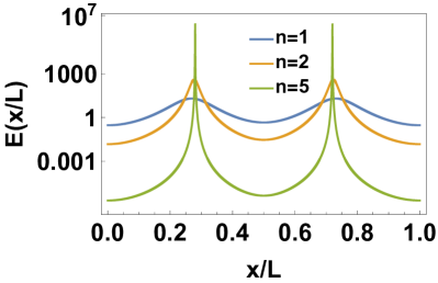
Figure 4: Left Panel: Plot of $E_{n}(x)$ as a function of $x$ for several representative values of $n$ in the heating phase with $\omega_{D}=3$ and$\delta f=0.04$. Right panel: Plot of $\delta x/L$, as a function of $\delta f$ for $\omega_{D}=100$. The peaks of $E_{n}(x)$ occur at $L/2\pm\delta x$. For all plots $\pi/L$ is set to unity and $f_{0}=10$. See text for details.

We note from Eq. 43 that for a generic $x$, $E_{n}(x)$ decays exponentially with $n$ with the large $n$ limit: $E_{n}(x)\sim e^{-4n\theta}$. This behavior can be in Fig. 4 where $E_{n}(x)$ is plotted for several $n$ as a function of $x$. The plot shows that $E_{n}(x)$, at large $n$, decays at all positions except at two places for which the leading terms of $Q_{1}^{2}(x)$ and $Q_{2}^{2}(x)$ in the large $n$ limit cancels each other. A straightforward calculation shows that

$$x_{c}^{\pm} = \frac{L}{2}\pm\delta x,\quad\delta x=\frac{L}{2\pi}\arccos(1/\alpha)$$ (44)

within first order FPT. Thus the position of the peaks of $E_{n}(x)$ in the large $n$ limit moves from $L/2$ to $L/4$ and $3L/4$ as one moves from the phase boundary to deep inside the heating phase. This behavior is supported for exact numerics as can be seen in the right panel of Fig. 4 where we plot the peak positions ($\pm\delta x/L$) as a function of $\delta f$ for $\hbar\omega_{D}=100(\pi/L)$.

In contrast for the non-heating phase we find using Eq. 24, $E_{n}(x)$, in real time, is given by Eq. 43 with $Q_{1}(x)\to Q^{\prime}_{1}(x)$ and $Q_{2}(x)\to Q^{\prime}_{2}(x)$, where

$$Q^{\prime}_{1}(x) = \alpha\cos\left(2\pi x/L\right)(1-\cos[2n\theta])+1-\alpha^{2}\cos[2n\theta]$$

$$Q^{\prime}_{2}(x) = \alpha\sqrt{\alpha^{2}-1}\sin\left(2\pi x/L\right)\sin[2n\theta]$$ (45)

Thus $E_{n}(x)$ is an oscillatory function of $n$ as shown in the left panel of Fig. 5 where $E_{n}(x)$ is plotted as a function of $x$ of several $n$.

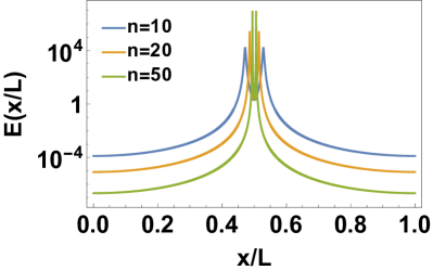
Figure 5: Left Panel: Plot of $E_{n}(x)$ as a function of $x$ for several representative values of $n$ in the non-heating phase ith $\omega_{D}=3$ and$\delta f=0.4$. Right panel: Same for $\omega_{D}=3$ and $\delta f=0.27$ when the system is almost on the transition line showing the development of a single peak at $x=L/2$ for large $n$ For all plots $\pi/L$ is set to unity and $f_{0}=10$. See text for details.

Finally on the transition line, using Eq. 25, we find

$$E_{n}(x) = \left(\frac{2\pi}{L}\right)^{2}h\frac{2(Q"_{1}^{2}(x)+Q"_{2}^{2}(x))}{(Q"_{1}^{2}(x)-Q"_{2}^{2}(x))^{2}}$$

$$Q"_{1}(x) = 1+2n^{2}s^{2}(1+\cos(2\pi x/L))$$

$$Q"_{2}(x) = 2sn\sin(2\pi x/L)$$ (46)

where we have analytically continued to real time. Thus we find the peak of $E_{n}(x)$ in the large $n$ limit occurs at $x=L/2$ for which $Q"_{1}(x)=1$ and $Q"_{2}(x)=0$. In contrast, for $x=0,L$, we have $Q"_{1}(x)=1+4n^{2}s^{2}$ and $Q"_{2}(x)=0$, so that $E_{n}(x)\sim 1/(1+4n^{2}s^{2})^{2}$ for all $n$. This behavior is consistent with the fact that $n^{\prime}_{c}$ diverges at the transition. A plot of $E_{n}(x)$ as a function of $x$ for several $n$, shown in the right panel of Fig. 5, confirms this behavior.

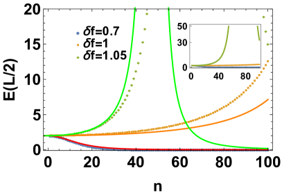
Figure 6: (Color online) Left Panel: Plot of $E_{n}(L)$ as a function of $n$ in the heating ($\delta f=0.7$, blue points), non-heating ($\delta f=1.1$, green points) phase, and on the transition line ($\delta f=1$, orange points). The solid lines shows the scaling law$1/(1+\mu n^{2})^{2}$. The inset shows results obtained using first order FPT. Right panel: Plot of $E_{n}(L/2)$ as a function of $n$ showing different behavior for $E_{n}(L/2)$ in the heating phase ($\delta f=0.7$, blue points), non-heating phase ($\delta f=1.05$, yellow points) and on the transition line ($\delta f=1$, yellow points). The solid lines shows the scaling law $1/(1+\mu^{\prime}n^{2})^{2}$ for each case. For the heating phase the color of the solid line is red for enhanced visibility. Here we have used $f_{0}=10$ $\omega_{D}=100$ and $\pi/L$ has been set to unity for all plots. See text for details.

We also note that $E_{n}(x)$ takes particulary simple forms at the center and end of the chains where it is given by

$$E_{n}(0) = E_{n}(L)=\left(\frac{2\pi}{L}\right)^{2}\frac{2(\alpha-1)^{2}h}{(\alpha\cosh[2n\theta]-1)^{2}}$$

$$E_{n}(L/2) = \left(\frac{2\pi}{L}\right)^{2}\frac{2(\alpha+1)^{2}h}{(\alpha\cosh[2n\theta]+1)^{2}}$$ (47)

From Eq. 47, we once again find the existence of a crossover timescale $n^{\prime}_{c}=n_{c}\sqrt{(1+\alpha)/(1+4\alpha)}$ below which $E_{n}(0)$ decays as $1/(1+\mu n^{2})^{2}$ where $\mu=2s^{2}\alpha(1+\alpha)$. This behavior is verified in the left panel of Fig. 6 which shows the behavior of $E_{n}(0)$ (with $E_{n}(0)=E_{n}(L)$) as a function of $n$; we find that the curves for the heating and non-heating phase become identical to the transition line for $n\neq n^{\prime}_{c}$. For $n\gg n^{\prime}_{c}$, the decay becomes exponential in the heating phase. In contrast, for $E_{n}(L/2)$, plotted in the right panel of Fig. 6, there is a clear distinction between behavior of $E_{n}$ in the heating phase and on the transition line. This can be attributed to the fact that $x=L/2$ coincides with the position of the peak on the transition line, while $E_{n}(L/2)$ decays in the heating phase.

III.2 Correlation functions

In this subsection, we present results for both equal-time and unequal-time correlation functions of primary operators and the stress tensor.

III.2.1 Equal time correlation function

We begin with the analysis of the equal-time correlation function starting from the asymptotic state $|h,\bar{h}\rangle$ given by

$$C_{n}(x_{1},x_{2}) = \frac{\langle h,\bar{h}|U^{\dagger n}\phi(w_{1},\bar{w}_{1})\phi(w_{2},\bar{w}_{2})U^{n}|h,\bar{h}\rangle}{\langle h,\bar{h}|h,\bar{h}\rangle}$$

(48)

where $w_{j}(\bar{w}_{j})=+(-)ix_{j}$ for $j=1,2$.

We first compute the holomorphic part of $C_{n}(x_{1},x_{2})$ which is given by

$$C_{n}^{\rm hol}(x_{1},x_{2})=\frac{\langle h|U^{n}\phi(w_{1})\phi(w_{2})U^{n}|h,\rangle}{\langle h|h\rangle}$$ (49)

$$= \lim_{z_{3}\to\infty,z_{4}\to 0}\prod_{j=1,2}\left(\frac{\partial w_{j}}{\partial z_{j}}\right)^{-h}\prod_{j=1,2}\left(\frac{\partial z_{jn}}{\partial z_{j}}\right)^{h}$$

$$\times z_{3}^{2h}{\langle 0|\phi(z_{3})\phi(z_{n1})\phi(z_{n2})\phi(z_{4})|0\rangle}$$

where $z_{jn}=(\tilde{a}_{n}z_{j}+\tilde{b}_{n})/(\tilde{c}_{n}z_{j}+\tilde{d}_{n})$. Here we choose the dimension of the primary fields $\phi$ to be same that of the state $|h\rangle$. The anti-holomorphic part an be written similarly in terms of $\bar{z}$ and $\bar{z}_{jn}$. To compute the four-point correlators of the primary fields, we use the standard result which expresses these in terms of the cross ratio of the complex coordinates $z_{i}$. To this end, we define $z_{ij}=z_{i}-z_{j}$ with $z_{k}=z_{kn}$ for $k=1,2$. Using this notation, we define the cross ratio

$$\eta = \frac{z_{31}z_{24}}{z_{32}z_{14}}=\frac{(z_{3}-z_{1n})(z_{2n}-z_{4})}{(z_{3}-z_{2n})(z_{1n}-z_{4})}$$ (50)

We note that for $z_{3}\to\infty$ and $z_{4}\to 0$, we have

$$\eta\to y_{n}(x_{1},x_{2})=\frac{z_{2n}}{z_{1n}}$$ (51)

$$=\frac{(\tilde{a}_{n}e^{i\pi x_{2}/L}+\tilde{b}_{n}e^{-i\pi x_{2}/L})(\tilde{c}_{n}e^{i\pi x_{1}/L}+\tilde{d}_{n}e^{-i\pi x_{1}/L})}{(\tilde{a}_{n}e^{i\pi x_{1}/L}+\tilde{b}_{n}e^{-i\pi x_{1}/L})(\tilde{c}_{n}e^{i\pi x_{2}/L}+\tilde{d}_{n}e^{-i\pi x_{2}/L})}$$

A similar result for $\bar{y}_{n}$ can be obtained for the anti-holomorphic part by replacing $x_{i}\to-x_{i}$.

To compute the four-point correlator, we first define the quantity

$${\mathcal{C}}_{n} = \lim_{z,{\bar{z}}\to\infty}z^{2h}{\bar{z}}^{2\bar{h}}\langle 0|\phi(z,\bar{z})\phi(z_{1n},\bar{z}_{1n})$$ (52)

$$\times\phi(z_{2n},\bar{z}_{2n})\phi(0,0)|0\rangle$$

To evaluate this, we first note that in the non-heating phase and on the transition line, $|1-z_{2n}/z_{1n}|,|1-\bar{z}_{2n}/\bar{z}_{1n}|\to 0$ for large $n$ in Euclidean time. To take advantage of this limit, we make the conformal transformation (where $z_{1}\equiv z_{1n}$ and $z_{2}\equiv z_{2n}$)

$$z_{i}\to z^{\prime}_{i}=-\frac{z(z_{i}-z_{2n})}{(z_{1n}-z_{i})z_{2n}}$$ (53)

so that in the new coordinate $z^{\prime}_{2n}=0$. A similar transformation is done for $\bar{z}_{i}$. Then using the standard transformation rule of operators $\phi(z,\bar{z})\to(\partial z^{\prime}_{i}/\partial z_{i})^{-h}(\partial z^{\prime}_{i}/\partial z_{i})^{-h}\phi(z^{\prime}_{i})$, one can write, after some straightforward algebra cftlit

$${\mathcal{C}}_{n} = z_{1n}^{-2h}\bar{z}_{1n}^{-2\bar{h}}{\mathcal{F}}(1-y_{n};1-\bar{y}_{n})$$ (54)

where $y_{n}=z_{2n}/z_{1n}$ and $\bar{y}_{n}=\bar{z}_{2n}/\bar{z}_{1n}$. The advantage of using this form for ${\mathcal{F}}$ which admits conformal block decomposition is that one can write down a perturbative expansion of the blocks around $|1-y_{n}|,|1-\bar{y}_{n}|=0$. This allows us to obtain an analytic, albeit perturbative expression of $C_{n}(x_{1},x_{2})$ for arbitrary $h,\bar{h}$. For the driven problem, $|1-y_{n}|,|1-\bar{y}_{n}|\ll 0$ (in Euclidean time) in the non-heating phase and on the transition line for all $x_{1},x_{2}$ in the large $n$ limit. Also, for all phases, this limit holds for all $n$ only for $|x_{1}-x_{2}|/L\ll 1$. The perturbative results that we chart out next is expected to be accurate in these limits. For the present case, one obtains cftlit2

$${\mathcal{F}} = \sum_{p}C_{hhp}^{2}\mathcal{V}_{p}(y_{n},h)\bar{\mathcal{V}}_{\bar{p}}(\bar{y}_{n},\bar{h})$$

$$\mathcal{V}_{p}(y_{n},h) = (1-y_{n})^{h_{p}-2h}\sum_{k}F_{k}(1-y_{n})^{k},\quad\bar{\mathcal{V}}_{\bar{p}}(\bar{y}_{n},\bar{h})=(1-\bar{y}_{n})^{\bar{h}_{p}-2\bar{h}}\sum_{k}F_{k}(1-\bar{y}_{n})^{k}$$

$$\sum_{k}F_{k}x^{k} = 1+\frac{h_{p}}{2}x+\frac{h_{p}\left(h_{p}\left(h_{p}\left(c_{0}+8h_{p}+8\right)+2(c_{0}+4h-4)\right)+c_{0}+8h(2h-1)\right)+8h^{2}}{8h_{p}\left(c_{0}+8h_{p}-5\right)+4c_{0}}x^{2}+{\mathcal{O}}(x^{3})$$ (55)

where $\sum_{p}$ denotes sum over primaries and $\mathcal{V}_{p}$ denotes the $p$-th conformal block with dimensions $h_{p},\bar{h}_{p}$ and the coefficients $C_{hhp}$ that depend on the details of the CFT. We note here that the identity block corresponds to $h_{p}=0$ and for this block $C_{hhI}=1$.

Substituting Eq. 55 in Eq. 49 (and its corresponding anti-holomorphic part), one obtains

$$\frac{C_{n}(x_{1},x_{2})}{C_{0}(x_{1},x_{2})} = \sum_{p}C_{hhp}^{2}(1-y_{n})^{h_{p}}(1-\bar{y}_{n})^{\bar{h}_{p}}$$ (56)

$$C_{0}(x_{1},x_{2}) = \left(\frac{2\pi}{L}\right)^{2(h+\bar{h})}\frac{(z_{1}z_{2})^{h}}{(z_{1}-z_{2})^{2h}}\frac{(\bar{z}_{1}\bar{z}_{2})^{\bar{h}}}{(\bar{z}_{1}-\bar{z}_{2})^{2\bar{h}}}$$

where only the leading term of the $\sum_{k}F_{k}x^{k}\simeq 1$ is retained.

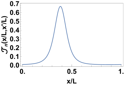
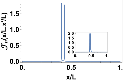
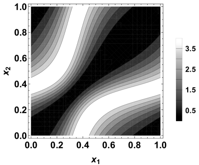
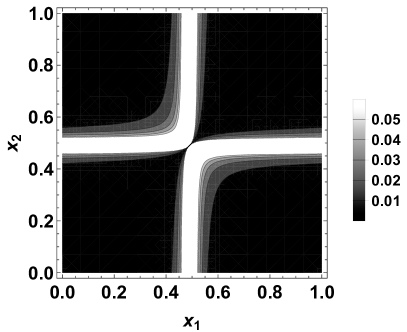
Figure 7: (Color online) Top left Panel: Plot of ${\mathcal{J}}_{n}(x_{1},x_{2})=(C_{n}(x_{1},x_{2})_{\rm univ}/C_{0}(x_{1},x_{2})-1)/(2h^{2}/c_{0})$ as a function of $x_{1}/L\equiv x/L$ in the non-heating phase ($\delta f=1.5$, $\omega_{D}=100$) for $x^{\prime}/L=x/L+0.03$ and $n=100$. Top Right panel: Similar plot for the heating phase ($\delta f=1.1$). The inset shows the behavior of the correlation function on the transition line ($\delta f=1$). Bottom left panel: Plot of ${\mathcal{J}}_{n}(x_{1},x_{2})$ as a function of $x_{1}$ and $x_{2}$ in the non-heating phase for $n=100$ showing emergence of spatial structure. Bottom right panel: Similar to the top left panel but for $\delta f=1$ where the system is on the transition line. Here we have used $f_{0}=10$ $\omega_{D}=100$ and $\pi/L$ has been set to unity for all plots. See text for details.

Next, we discuss the contribution of the identity block which is universal since $C_{hhI}=1=C_{\bar{h}\bar{h}I}$. For this block, $h_{p}=\bar{h}_{p}=0$. We note that if we retain only the first order term, we find from Eq. 56 that $C_{n}(x_{1},x_{2})$ becomes independent of $n$. The first non-trivial contribution of the identity block arises from the $x^{2}$ term in the expansion of $\sum_{k}F_{k}x^{k}$. This universal contribution is given by

$$\frac{C_{n}(x_{1},x_{2})_{\rm univ}}{C_{0}(x_{1},x_{2})} = 1+\frac{2h^{2}}{c_{0}}{\rm Re}[(1-y_{n})^{2}]$$ (57)

Thus in this limit, the identity block contribution to the deviation of $C_{n}$ from its equilibrium value provides a measure of the central charge. A plot of ${\mathcal{J}}_{n}(x_{1},x_{2})=(C_{n}(x_{1},x_{2})_{\rm univ}/C_{0}(x_{1},x_{2})-1)/(2h^{2}/c_{0})$ (after analytic continuation to real time) is shown in the top panels of Fig. 7 as a function $x_{1}/L=x/L$ for $x_{2}/L=x_{1}/L+0.03$ after $n=100$ cycles of the drive. For these plots we have chosen $\hbar\omega_{D}=100\pi/L$. The top left panel shows the behavior of $C_{n}(x_{1},x_{2})_{\rm univ}$ in the non-heating phase ($\delta f=1.5$) displaying a broad oscillatory structure. In contrast, in the top right panel, for the heating phase ($\delta f=0.9$) it displays two sharp peaks consistent with the behavior of $E_{n}(x)$. The position of these peaks shift to $L/2$ on the transition line as can be seen from the inset of top right panel of Fig. 7. The bottom panels show the behavior of $C_{n}(x_{1},x_{2})_{\rm univ}$ for large $n=100$ in the non-heating phase (left panel) and on the transition line (right panel) where the perturbative expansion of ${\mathcal{F}}$ is expected to be accurate. We find clear emergence of spatial pattern in the non-heating phase in contrast to the behavior of $E_{n}$. We shall discuss this behavior in more details in the context of unequal-time correlation function.

In the large central charge $c_{0}$ limit, with the conformal dimensions held fixed, the Virasoro conformal blocks reduce to global conformal blocks which are given in terms of hypergeometric functions, by cftlit6 ,

$$\mathcal{V}_{p}(x) = x^{h_{p}-2h}\,{}_{2}F_{1}\left(h_{p},h_{p};2h_{p};x\right)+{\mathcal{O}}(1/c).$$ (58)

Hence the correlator is given by

$$\frac{C_{n}(x_{1},x_{2})}{C_{0}(x_{1},x_{2})}\simeq\sum_{p\neq\mathbb{I}}C_{hhp}^{2}(1-y_{n})^{h_{p}}(1-\bar{y}_{n})^{\bar{h}_{p}}$$ (59)

$$\times{}_{2}F_{1}\left(h_{p},h_{p};2h_{p};1-y_{n}\right){}_{2}F_{1}\left(\bar{h}_{p},\bar{h}_{p};2\bar{h}_{p};1-\bar{y}_{n}\right).$$

where $C_{0}(x_{1},x_{2})$ is defined in Eq. 56. Note that since the Virasoro blocks reduce to global block in this limit, there is no identity block, i.e., $h_{p}\neq 0$.

Finally, we note for CFTs with large central charge $c_{0}\gg 1$, when the asymptotic states have large conformal dimension $H\gg h$, with $h/c_{0}$ and $H/c_{0}$ both held fixed, a closed form answer is available via the monodromy methods. Therefore we compute the equal-time correlation function $C^{\prime}_{n}(x_{1},x_{2})=\langle H,\bar{H}|\phi(w_{1},\bar{w}_{1})\phi(w_{2},\bar{w}_{2})|H,\bar{H}\rangle/\langle H,\bar{H}|H,\bar{H}\rangle$. This can be done exactly in the same way as charted out above; the only difference is that one needs to keep track of two operator dimension $H$ and $h$. A straightforward calculation shows that in this case one has cftlit3

$${\mathcal{V}}_{p}(z_{1n},z_{2n},h) = \left(\frac{a_{0}(z_{1n}z_{2n})^{(a_{0}-1)/2}}{z_{1n}^{a_{0}}-z_{2n}^{a_{0}}}\right)^{2h}$$ (60)

$$\times\left(\frac{4(1-y_{n}^{a_{0}/2})}{a_{0}(1+y_{n}^{a_{0}/2})}\right)^{h_{p}}$$

with $a_{0}=\sqrt{1-24H/c_{0}}$. A similar expression can be obtained for $\bar{\mathcal{V}}_{\bar{p}}$ by substituting $z_{jn}\to\bar{z}_{jn}$ and $h,h_{p}\to\bar{h},\bar{h}_{p}$. One can then write $C_{n}$ in terms of ${\mathcal{V}}_{p}$ and $\bar{\mathcal{V}}_{p}$ as

$$C^{\prime}_{n}(x_{1},x_{2}) = \left(\frac{2\pi}{L}\right)^{2(h+\bar{h})}\sum_{p}C^{2}_{hhp}{\mathcal{V}}_{p}(z_{1n},z_{2n},h)$$ (61)

$$\times\bar{\mathcal{V}}_{\bar{p}}(\bar{z}_{1n},\bar{z}_{2n},\bar{h})\left({z_{1}z_{2}}\right)^{h}\left({\bar{z}_{1}\bar{z}_{2}}\right)^{\bar{h}}.$$

A motivation for studying such large $c_{0}$ CFTs comes from the AdS/CFT correspondence. These are CFTs which are expected to have semiclassical gravity duals. The global block answer for light correlators is reproduced in bulk AdS by the geodesic Witten diagrams cftlit7 . The Virasoro vacuum block is non-trivial in two dimensions unlike its higher dimensional versions as it contains the stress tensor and its descendants. In the large $c_{0}$ limit, the dynamics of the Virasoro vacuum block matches with results from semiclassical gravity cftlit3 . In CFT₂, since one has Virasoro, one can use the geodesic Witten diagrams to interpolate between the global and the semiclassical monodromy answer (when pair of operator conformal dimensions scale with the central charge) by taking into account backreaction due to the heavy geodesicscftlit8 . The time-dependent drive of an inhomogeneous metric will have implications for the physics of black holes in the dual gravitational theory. We are not going to explore this issue further here.

III.2.2 Unequal time correlation function

In this subsection, we compute the unequal-time correlation function of the primary fields $G_{n}(x_{1},x_{2})$. We note that unequal-time correlation functions of the vacuum state, unlike-their equal-time counterparts, display non-trivial dynamics cft3 . In what follows, we chart out the result for these correlation functions for the CFT vacuum given by

$$G_{n}(x_{1},x_{2}) = \langle 0|\phi(w_{1},\bar{w}_{1})U_{n}^{\dagger}\phi(w_{2},\bar{w}_{2})U^{n}|0\rangle$$

The holomorphic part of this correlator yields after mapping to the complex plane,

$$G_{n}^{\rm hol}(x_{1},x_{2}) = \prod_{j=1,2}\left(\frac{\partial w_{j}}{\partial z_{j}}\right)^{-h}\left(\frac{\partial z_{n2}}{\partial z_{2}}\right)^{h}\frac{1}{(z_{n2}-z_{1})^{2h}}$$

$$= \left(\frac{2\pi}{L}\right)^{2h}\frac{(z_{1}z_{2})^{h}}{\left(\tilde{a}_{n}z_{2}+\tilde{b}_{n}-\tilde{c}_{n}z_{1}z_{2}-\tilde{d}_{n}z_{1}\right)^{2h}}$$

The antiholomorphic part can be computed in a similar manner with $z_{i}\to\bar{z}_{i}$. Thus one finally gets for $h=\bar{h}$

$$G_{n}(x_{1},x_{2}) = \left(\frac{2\pi}{L}\right)^{4h}\frac{1}{|\tilde{a}_{n}z_{2}+\tilde{b}_{n}-\tilde{c}_{n}z_{1}z_{2}-\tilde{d}_{n}z_{1}|^{4h}}$$

where $z_{i}=\exp[2\pi ix_{i}/L]$. Defining the dimensionless center of mass and relative coordinates as $x_{\rm cm}=\pi(x_{1}+x_{2})/L$ and $x_{\rm rel}=\pi(x_{1}-x_{2})/L$, analytically continuing to real time, and substituting Eqs. 23, 24 and 25 in Eq. LABEL:uetcft3, one obtains

$$G_{n}(x_{\rm cm},x_{\rm rel}) = \left(\frac{\pi}{2L}\right)^{4h}\left[\left(\alpha\cos(x_{\rm cm})+\cos(x_{\rm rel})\right)\sinh(n\theta)+\sqrt{\alpha^{2}-1}\cosh(n\theta)\sin(x_{\rm rel})\right]^{-4h}\quad{\rm heating}$$

$$= \left(\frac{\pi}{2L}\right)^{4h}\left[\left(\alpha\cos(x_{\rm cm})+\cos(x_{\rm rel})\right)\sin(n\theta)+\sqrt{1-\alpha^{2}}\cos(n\theta)\sin(x_{\rm rel})\right]^{-4h}\quad{\rm non-heating}$$

$$= \left(\frac{\pi}{2L}\right)^{4h}\Big{|}ns[\cos(x_{\rm cm})+\cos(x_{\rm rel})]\Big{|}^{-4h}\,{\rm transition\,line}$$

where we have assumed $h=\bar{h}$.

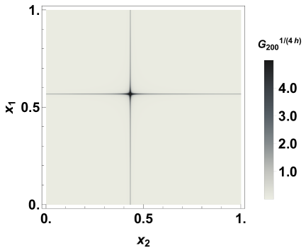
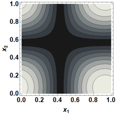
Figure 8: (Color online) Left Panel: Plot of $G$ after $n=10$ drive cycles for the heating phase($\omega_{D}=40$, $\delta f=0.98$) as a function of $x_{1}/L$ and $x_{2}/L$ showing the position of the peaks of $G_{n}$ in the of $x_{1}-x_{2}$ plane. Right panel: Plot of $f(x_{1},x_{2})=\alpha\cos x_{\rm cm}+\sqrt{2}\sin(x_{\rm rel}+\pi/4)$ as a function of $x_{1}/L$ and $x_{2}/L$ for the same parameter values showing the position of zeros(darker shades) almost coinciding with the position of peaks in the left panel. For all plots, $f_{0}=10$. See text for details.

A straightforward analysis of $G_{n}(x_{\rm cm},x_{\rm rel})$ in the heating phase reveals that it will display peaks, in the large $n$ limit, when

$$\cos(x_{\rm cm}) = -\sin(x_{\rm rel}+\arcsin(1/\alpha))$$ (66)

For $x_{\rm rel}=0$, we find that the peak position coincide with those of $E_{n}(x)$. In general, the position of the peaks trace a curve in the $(x_{1},x_{2})$ space and can be tuned by changing $\alpha$; for $\alpha\to\infty$, the peaks only occurs when $x_{\rm cm}=x_{\rm rel}+\pi/2$. Thus this phenomenon constitutes another example of emergence of spatial structure in driven CFTs which was initially found by analysis of $E_{n}(x)$ cft4 . For all pairs of values $(x_{1},x_{2})$ which do not satisfy Eq. 66, $G_{n}$ decays exponentially with $n$ in the large $n$ limit: $G_{n}\sim\exp[-4nh]$. This behavior is clearly seen in the left panel of Fig. 8 where $G_{n}(x_{1},x_{2})$ is plotted as a function of $x_{1}/L$ and $x_{2}/L$. The position of the divergence of $G_{n}(x_{1},x_{2})$ coincides with the solution of Eq. 66 as can be seen from the right panel of Fig. 8.

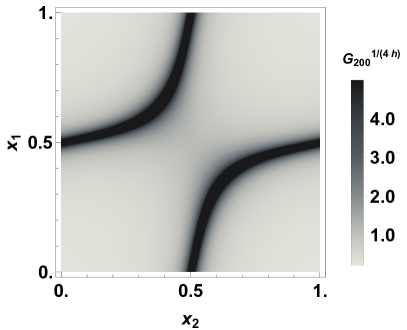
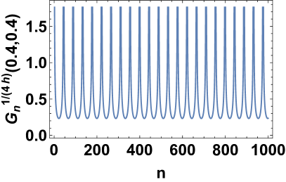
Figure 9: (Color online)Left Panel: Plot of $G_{n}(x_{1},x_{2})$ after $n=10$ drive cycles for the non- heating phase ($\omega_{D}=100$,$\delta f=1.5$). Right panel: Plot of $G_{n}(x_{1}=0.4L,x_{2}=0)$ as a function of $n$ for $\omega_{D}=100$ and $\delta f=1.5$ showing multiple divergences as a function of $n$ as predicted by Eq. 67. For all points $f_{0}=10$ and $\pi/L$ is set to unity. See text for details.

In contrast, the peaks of $G_{n}(x_{1},x_{2})$ in the non-heating phase do not occur at an fixed positions independent of $n$ in the large $n$ limit. Here the divergences for occur when $n\theta=m\pi$ (for integer $n$ and $m$) if $x_{1}=x_{2}$; for all $x_{1}\neq x_{2}$, they occur when $n$, $x_{1}$, and $x_{2}$ satisfies

$$\frac{\alpha\cos(x_{\rm cm})+\cos(x_{\rm rel})}{\sqrt{1-\alpha^{2}}\sin(x_{\rm rel})} = -\cot(n\theta)$$ (67)

These divergences constitute emergent spatial singularities of the unequal time correlation function in the non-heating phases and have no analog in energy density of the system. Such divergences, which also showed up for equal-time correlation function in the botom left panel of Fig. 8, can be clearly seen in the left panel of Fig. 9 where $[G_{n}(x_{1},x_{2})]^{1/4h}$ is plotted as a function of $x_{1}$ and $x_{2}$ for $n=30$. The right panel shows multiple divergences of $G_{n}^{4(h+\bar{h})}$ for $x_{1}=0.4$ and $x_{2}=0$ as a function of $n$. Finally, we note that on the transition line $G_{n}(x_{1},x_{2})$ can diverge if $\cos(x_{\rm cm})=-\cos(x_{\rm rel})$, i.e., for $x_{1}=L/2$ or $x_{2}=L/2$. On the transition line, for large $n$ one finds a $1/n^{4(h+\bar{h})}$ decay of the correlator for all $(x_{1},x_{2})$ except when $x_{1}=L/2$ or $x_{2}=L/2$ in which case it diverges. The behavior of $G_{n}(x_{1},x_{2})$ on the transition line as a function of $x_{1}$ and $x_{2}$ is shown in the left panel of Fig. 10 showing line of divergences at $x_{1}=L/2$ and $x_{2}=L/2$. For $x_{1},x_{2}\neq L/2$, $G_{n}^{1/4h}$ decays linearly with $n$ as shown in the right panel of Fig. 10 for $x_{1}/L=0.99$ and $x_{2}=0$. These features, obtained from exact numerics, confirms the analytic prediction of the first order FPT.

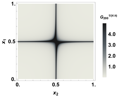
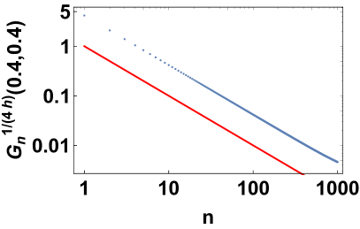
Figure 10: (Color online)Left Panel: Plot of $G_{n}^{1/4h}(x_{1},x_{2})$ after $n=10$ drive cycles when the system is on the transition line ($\omega=100$,$\delta f=1$). Right panel: Plot of $G_{n}^{1/4h}(x_{1}=0.99L,x_{2}=0)$ as a function of $n$ for $\omega_{D}=100$ and $\delta f=1$ showing linear decay with $n$. The blue dots indicate values of $G_{n}^{1/4h}$ while the red line is the linear fit. For all points $f_{0}=10$ and $\pi/L$ is set to unity. See text for details.

III.3 Entanglement

In this subsection, we consider the evolution of the $m^{\rm th}$ Renyi entropy $S_{n}^{m}$ after $n$ drive cycles starting from $|h,\bar{h}\rangle$ states. We note that the ground state has $S_{n}^{m}=S_{0}^{m}$ since the state does not change under the drive in the cylindrical geometry. This entanglement can be computed most simply by considering the correlation of the twist operators ${\mathcal{T}}(w,\bar{w})$ cardyref1 . Here we shall concentrate on the $m^{\rm th}$ Renyi entropy which is given, after $n$ cycles of the drive, in terms of the twist operator ${\mathcal{T}}_{m}(w,\bar{w})$ as

$$S_{n}^{m}(\ell) = \frac{1}{1-m}\ln\alpha_{n}^{m}(\ell),\quad\alpha_{n}^{m}(\ell)={\rm Tr}\rho_{n}^{m}(\ell)$$

$$\alpha_{n}^{m}(\ell) = \frac{\langle h,\bar{h}|U^{n\dagger}{\mathcal{T}}(w_{1},\bar{w}_{1}){\mathcal{T}}(w_{2},\bar{w}_{2})U^{n}|h,\bar{h}\rangle}{\langle h,\bar{h}|h,\bar{h}\rangle}$$ (68)

where $\rho_{n}(\ell)$ is the reduced density matrix of state after $n$ cycles of the drive corresponding to an initial state $|h,\bar{h}\rangle$, $\ell$ is the spatial dimension of the subsystem, $w_{i}(\bar{w}_{i})=+(-)ix_{i}$, we choose $x_{1}=0$ and $x_{2}=\ell$, and the twist operator ${\mathcal{T}}_{m}$ represents a primary field with dimension $h_{m}=c(m-1/m)/24$ cardyref1 . In what follows, we shall focus on the half-chain entanglement entropy which corresponds to $\ell=L/2$ for the sake of simplicity; we note however, that the method can yield results for arbitrary $\ell$.

As before we evaluate the holomorphic part of the $\alpha_{n}^{m}(\ell=L/2)$. This is given by

$$\alpha_{n}^{m} = \lim_{z_{3}\to\infty,z_{4}\to 0}\left(\frac{2\pi}{L}\right)^{2h_{m}}\frac{C_{4n}^{m\rm hol}e^{\pi ih_{m}}}{\left(\tilde{d}_{n}^{2}-\tilde{c}_{n}^{2}\right)^{2h_{m}}}$$

$$C_{4n}^{m\rm hol} = \lim_{z\rightarrow\infty}z^{2h}\langle 0|\phi(z){\mathcal{T}_{m}}(z_{n1}){\mathcal{T}_{m}}(z_{n2})\phi(0)|0\rangle$$ (69)

The computation of $C_{4n}^{m}=C_{4n}^{m\,\rm hol}C_{4n}^{m\,\rm anti-hol}$ and hence $S_{n}^{m}$ thus reduce to a problem similar to that worked out for the correlation function. However, here the operator dimension of ${\mathcal{T}}_{m}$ are different from $h$, and hence all the expressions obtained in Sec. III.2 can not be directly used. Nevertheless, the computation procedure is similar, and we present the main results here. We find that $C_{4n}^{m}$ can once again be written in terms of sum of contribution over conformal blocks. In the perturbative limit, where $|1-y_{n}|,|1-\bar{y}_{n}|\ll 1$, one has

$$C_{4n}^{m}=z_{1n}^{-h-h_{m}}\bar{z}_{1n}^{-\bar{h}-\bar{h}_{m}}{\mathcal{F}}^{\prime}(1-y_{n};1-\bar{y}_{n}),\quad{\mathcal{F}}^{\prime}=\sum_{p}C_{hhp}C_{h_{m}h_{m}p}\mathcal{V}_{p}\bar{\mathcal{V}}_{\bar{p}}$$ (70)

$$\mathcal{V}_{p}(y_{n},h,h_{m})=(1-y_{n})^{h_{p}-h-h_{m}}\sum_{k}F_{k}(1-y_{n})^{k},\quad\bar{\mathcal{V}}_{\bar{p}}(\bar{y}_{n},\bar{h},\bar{h}_{m})=(1-\bar{y}_{n})^{\bar{h}_{p}-\bar{h}-\bar{h}_{m}}\sum_{k}F_{k}(1-\bar{y}_{n})^{k},$$

$$\sum_{k}F_{k}x^{k}=1+\frac{h_{p}}{2}x+\frac{h_{p}\left(h_{p}\left(h_{p}\left(c+8h_{p}+8\right)+2(c+2h-4)\right)+c-4h\right)+4h_{m}\left(h_{p}\left(h_{p}+4h-1\right)+2h\right)}{8h_{p}\left(c+8h_{p}-5\right)+4c}x^{2}+{\mathcal{O}}(x^{3})$$

We note that this perturbative result is expected to be accurate for large $n$ and in the non-heating phases or on the transition line as discussed earlier. Also in these cases since $|1-y_{n}|,|1-\bar{y}_{n}|\ll 1$, only the leading term in the sum may be retained. Substituting Eq. 70 in Eq. 69 and after some straightforward algebra one obtains, assuming $h=\bar{h}$ and using $h_{m}=\bar{h}_{m}$

$$\alpha_{n}^{m}(L/2)\simeq\left(\frac{2\pi}{L}\right)^{4h_{m}}\sum_{p}C_{hhp}C_{h_{m}h_{m}p}4^{\tfrac{h_{p}+\bar{h}_{p}}{2}-h_{m}-h}\left(\frac{\tilde{a}_{n}+\tilde{b}_{n}}{c_{n}+d_{n}}\right)^{\bar{h}_{p}-h_{p}}|\tilde{c}_{n}^{2}-\tilde{d}_{n}^{2}|^{2(h-h_{m})}(\tilde{d}_{n}^{2}-\tilde{c}_{n}^{2})^{-h_{p}}(\tilde{a}_{n}^{2}-\tilde{b}_{n}^{2})^{-\bar{h}_{p}}$$

(71)

If we retain only the identity contribution which is universal, then using $C_{aaI}=1$ we can simplify,

$$\alpha_{n}^{m}(L/2)_{\rm univ} \simeq \left(\frac{2\pi}{L}\right)^{4h_{m}}4^{-h_{m}-h}$$ (72)

$$\times|\tilde{c}_{n}^{2}-\tilde{d}_{n}^{2}|^{2(h-h_{m})}$$

This universal contribution, after analytic continuation to real time, yields a simple expression for the evolution of $\delta S_{n}^{m}=S_{n}^{m}-S_{n=0}^{m}$, given by

$$\delta S_{n}^{m}(L/2)_{\rm univ}\simeq\frac{2(h-h_{m})}{1-m}\ln|c_{n}^{2}-d_{n}^{2}|$$ (73)

In the non-heating phase and on the transition line, this yields, after analytic continuation to real time,

$$\delta S_{n}^{m}(L/2)_{\rm univ} \simeq \frac{h-h_{m}}{1-m}\ln\Big{[}\left(1+\alpha^{2}\cos 2n\theta\right)/\sqrt{1-\alpha^{2}}\Big{]},\quad{\rm non-heating}$$ (74)

$$\simeq \frac{h-h_{m}}{1-m}\ln(1+4n^{2}s^{2}),\quad{\rm transition\,line}$$

Thus the oscillatory behavior of $\delta S_{n}$ in the non-heating phase and its logarithmic growth on the transition line are expected qualitative features that are reproduced in this perturbative approach. We note that the linear growth of the entanglement in the hyperbolic phase is also reproduced by this procedure; however, here we can not ascertain the accuracy of this result since the perturbation expansion of ${\mathcal{F}}$ over conformal blocks are uncontrolled.

In the large central charge limit, for states with fixed conformal dimensions, we can use the global block approximation to express (assuming $h_{m}=\bar{h}_{m}$ and $h=\bar{h}$)

$$\alpha_{n}^{m}(L/2)\simeq\left(\frac{2\pi}{L}\right)^{4h_{m}}\sum_{p\neq{\mathbb{I}}}C_{hhp}C_{h_{m}h_{m}p}4^{\tfrac{h_{p}+\bar{h}_{p}}{2}-h_{m}-h}\left(\frac{\tilde{a}_{n}+\tilde{b}_{n}}{\tilde{c}_{n}+\tilde{d}_{n}}\right)^{\bar{h}_{p}-h_{p}}(\tilde{d}_{n}^{2}-\tilde{c}_{n}^{2})^{-h_{p}}(\tilde{a}_{n}^{2}-\tilde{b}_{n}^{2})^{-\bar{h}_{p}}$$

$$\times|\tilde{c}_{n}^{2}-\tilde{d}_{n}^{2}|^{2(h-h_{m})}\times{}_{2}F_{1}\left(h_{p}-h+h_{m},h_{p}-h+h_{m};2h_{p};1-y_{n}\right){}_{2}F_{1}\left(\bar{h}_{p}-h+h_{m},\bar{h}_{p}-h+h_{m};2\bar{h}_{p};1-\bar{y}_{n}\right).$$ (75)

Defining $\alpha_{n}^{m0}(L/2)=(2\pi/L)^{4h_{m}}4^{-(h_{m}+h)}$ and $\delta S_{n}^{m}=\ln[\alpha_{n}^{m}(L/2)/\alpha_{n}^{m0}(L/2)]/(1-m)$, we find, using Eq. 75,

$$\delta S_{n}^{m}\simeq\frac{1}{1-m}\ln\Big{[}\sum_{p\neq{\mathbb{I}}}C_{hhp}C_{h_{m}h_{m}p}4^{\tfrac{h_{p}+\bar{h}_{p}}{2}}\left(\frac{\tilde{a}_{n}+\tilde{b}_{n}}{\tilde{c}_{n}+\tilde{d}_{n}}\right)^{\bar{h}_{p}-h_{p}}(\tilde{d}_{n}^{2}-\tilde{c}_{n}^{2})^{-h_{p}}(\tilde{a}_{n}^{2}-\tilde{b}_{n}^{2})^{-\bar{h}_{p}}$$ (76)

$$\times|\tilde{c}_{n}^{2}-\tilde{d}_{n}^{2}|^{2(h-h_{m})}\times{}_{2}F_{1}\left(h_{p}-h+h_{m},h_{p}-h+h_{m};2h_{p};1-y_{n}\right){}_{2}F_{1}\left(\bar{h}_{p}-h+h_{m},\bar{h}_{p}-h+h_{m};2\bar{h}_{p};1-\bar{y}_{n}\right).\Big{]}$$

This provides the drive induced contribution to the half-chain $m^{\rm th}$ Renyi entropy after $n$ drive cycles.

Finally we consider the case for large $c_{0}$ CFTs such that $h/c_{0}\gg h_{m}/c_{0}$ with $h/c_{0}$ and $h_{m}/c_{0}$ held fixed. Here once again, it is possible to obtain analytic expression of $\alpha_{n}^{m}(\tfrac{L}{2})$ using the monodromy block Eq. 60. The universal contribution (from the identity block) non-perturbative in $n$ is given by,

$$\alpha_{n}^{m}(L/2)_{\rm univ} = \left(\frac{2\pi a_{0}}{L}\right)^{4h_{m}}|c_{n}^{2}-d_{n}^{2}|^{-2h_{m}(a_{0}+1)}|a_{n}^{2}-b_{n}^{2}|^{2h_{m}(a_{0}-1)}\Big{|}\left(\frac{a_{n}+b_{n}}{c_{n}+d_{n}}\right)^{a_{0}}-\left(\frac{a_{n}-b_{n}}{c_{n}-d_{n}}\right)^{a_{0}}\Big{|}^{-4h_{m}}$$ (77)

$$\delta S_{n}^{m}(L/2)_{\rm univ} = \frac{1}{1-m}\Big{(}4h_{m}\ln\Big{|}\left(\frac{a_{n}+b_{n}}{c_{n}+d_{n}}\right)^{a_{0}}-\left(\frac{a_{n}-b_{n}}{c_{n}-d_{n}}\right)^{a_{0}}\Big{|}+2h_{m}(a_{0}+1)\ln|c_{n}^{2}-d_{n}^{2}|+2h_{m}(1-a_{0})\ln|a_{n}^{2}-b_{n}^{2}|.\Big{)}$$

where we have analytically continued to real time. We note here that the exact conformal block contribution can also be determined numerically using the Zamolodchikov recursion relations zamu ; however, we are not going to address this in this work.

IV Relation to lattice models

In this section, we relate our results obtain using conformal field theory in the last section to those obtained by exact numerics on a specific lattice model. The model chosen is the sine-square deformed (SSD) fermionic model whose Hamiltonian is given by ssdpapers ; cft1

$$H_{\rm SSD} = [H_{0}+(H_{+}+H_{-})/2]/2$$

$$H_{0} = -\sum_{j}J(c_{j}^{\dagger}c_{j+1}+{\rm h.c})$$ (78)

$$H_{\pm} = -\sum_{j}{J_{1}}e^{ij\delta}(c_{j}^{\dagger}c_{j+1}+{\rm h.c.})$$

where $c_{j}$ is the fermion annihilation operator on site $j$, $\delta=2\pi/L$, $L$ is the chain length, the lattice spacing is set to unity, we have assumed that the system to be at half-filling, and $J$ is the hopping strength of the fermions. In what follows, we shall use periodic boundary condition for this Hamiltonian. We note that due to the local phase factor $\exp[\pm i\delta j]$, $H_{\pm}$ are not Hermitian operators. However, their sum is still Hermitian and leads to

$$H_{\rm SSD} = -\sum_{j}J\Lambda_{j}(c_{j}^{\dagger}c_{j+1}++{\rm h.c.})=\sum_{j}h_{j}$$

$$\Lambda_{j} = 1+2J_{1}\cos\left(\frac{2\pi}{L}(j-1/2)\right)/J$$ (79)

where $J$ is the hopping strength of the fermions. In what follows, we shall implement the drive via a time-dependent hopping $J\to J(t)=J_{1}+J_{0}\cos(\omega_{D}t))+\delta J$. It is well known ssdpapers ; cft1 that the low-energy sector of Hamiltonian can be expressed as

$$H = \frac{2\pi}{L}(J(t)L_{0}+J_{1}(L_{1}+L_{-1})/2)$$ (80)

$$+{\rm anti-holomorphic\,part}$$

so that one can identify $\delta f=\delta J+J_{1}$ and $J_{0}=f_{0}$. In what follows, we shall scale all energies by $J_{1}$ and compute the time evolution of the instantaneous energy density of the system, $E_{n}(x)$ after $n$ cycles of the drive as follows.

To this end, we first compute $U(T,0)=T_{t}\exp[-i\int_{0}^{T}dtH_{\rm SSD}(t)/\hbar]$ numerically. The procedure for this identical to the one carried out in Sec. II and involves decomposition of $U$ into $N$ time steps of width $\delta t=T/N$: $U(T,0)=\prod_{j=0..N-1}U_{j}$, where $U_{j}=U(t_{j}+\delta t,t_{j})$. The width $\delta t$ is chosen such that $H_{\rm SSD}$ does not vary appreciably within this interval. One then diagonalizes $H_{j}$ and expresses $U_{j}$ in terms of its eigenvalues and eigenvectors. The matrix $U$ is then constructed by taking product over all $U_{j}$s. Finally one diagonalizes $U$ to obtain the Floquet eigenvalues $\epsilon_{m}^{F\,\rm SSD}$ and eigenvectors $|m_{\rm SSD}\rangle$. In terms of these after n drive cycles, the wavefunctions of the driven chain can be written as

$$|\psi_{n}\rangle = \sum_{m}e^{-i\epsilon_{m}^{F\,\rm SSD}nT/\hbar}c_{m}|m_{\rm SSD}\rangle$$ (81)

where $c_{m}=\langle m_{\rm SSD}|\psi_{\rm init}\rangle$ denotes the overlap of the Floquet eigenstates with the initial state. The initial state is chosen to be one of the primary CFT states; for the lattice model studied here, these states are tabulated in Ref. xxcft, . We note since $f_{0}\gg 1$, the initial primary states corresponding to $H_{\rm SSD}$ is expected to be accurately described by those charted in Ref. xxcft, . Here we choose the state corresponding to $h=\bar{h}=1/2$ which for the lattice correspond to the state

$$|\psi_{\rm init}\rangle = c_{k_{F}+\pi/L}^{\dagger}c_{-k_{F}-\pi/L}^{\dagger}|{\rm FS}\rangle$$ (82)

where $|{\rm FS}\rangle$ is the half-filled Fermi sea. Thus $|\psi_{\rm init}\rangle$ corresponds to two particles populating the lowest available energy states over the half-filled Fermi sea xxcft . One then computes the instantaneous energy density at any given site as $E_{n}(j)=\langle\psi_{\rm init}|h_{j}(n)|\psi_{\rm init}\rangle$, where $h_{j}(n)=U^{\dagger}(nT,0)h_{j}(t=0)U(nT,0)$. In what follows we shall study the behavior of $E_{n}(j)$ and relate it to the corresponding CFT results obtained in Sec. III.1.

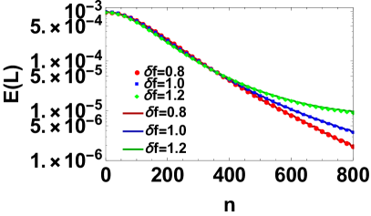
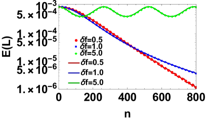
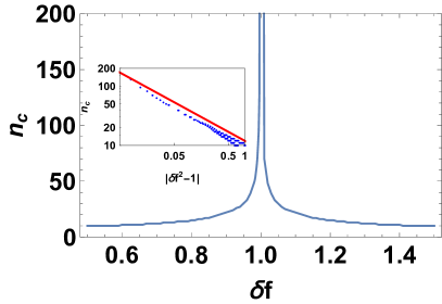
Figure 11: (Color online)Top Left Panel: Plot of $E_{n}(L)=E_{n}(0)$ as a function of $n$ as obtained from lattice (solid lines) and CFT (dotted lines) calculations showing universal behavior for $n\leq n_{c}\simeq 200$ for several representative values of $\delta f$ (in units of $\pi/L$). Top Right panel: Plot of $E(L)$ as a function of $n$ obtained from lattice (solid lines) and CFT (dotted lines) calculations showing deviation oscillatory and decaying behaviors in non-heating and heating phases and on the transition line. Bottom left panel: Plot of $E(x)$ as a function of $x$ after $n=1500$ drive cycles and $\delta f=5\pi/L\simeq 0.078$ showing the emergent spatial structure. Bottom Right panel: Plot of $n_{c}$ as a function of the $\delta f$ (in units of $\pi/L$) showing the divergence at the transition line. The inset shows plots of $\delta n_{c}$ vs $\delta f$ on log scale. The red line corresponds to a plot of $1/\sqrt{|\delta f^{2}-1|}$. For all points $\omega_{D}=40J_{1}/\hbar$ for which $\delta f_{c}\simeq\pi/L$ and we have chosen $L=202$. See text for details.

The results obtained from this procedure is shown in Fig. 11 for a chain of length $L=200$. The top left panel shows a plot of $E(L)$ as a function of $n$ for $\omega_{D}=40J_{1}/\hbar$ for several representative values of $\delta f$. At this frequency, the transition line is at $\delta f_{c}\simeq 1$. One therefore finds that below a threshold number of drive cycles, $n_{c}$, $E(L)$ as obtained from the lattice shows universal behavior for both the phases and mimics the behavior of the system on the transition line. Moreover, these results show an excellent match with the corresponding CFT results outlined in Eqs. 43, 45, and 46 (with $L$ in Eq. 1 identified to the chain length of the lattice Hamiltonian). The long time behavior of $E(L)$ as a function of $n$ in all the phases is shown in the top right panel of Fig. 11. We find that the lattice model reflects a clear distinction, as predicted by CFT, between the behavior of $E(L)$ in the heating and non-heating phases at long times (large $n$). The bottom left panel shows the energy density $E(x)$ as a function of $x/L$ in the heating phase corresponding to $\omega_{D}=40J_{1}/\hbar$ and $\delta f=5\pi/L$ after $n=1500$ cycles of the drive. We find that the peak positions predicted by CFT are correctly captured by the lattice model; however, the peak amplitudes are lower which is due to lattice effects that are expected to cause deviation of lattice dynamics from the CFT results in the heating phase at large $n$ cft2 . Finally, in the bottom right panel of Fig. 11, we find that $n_{c}$ diverges at the transition; this divergence seems to coincide with the predicted $1/\sqrt{|1-\alpha^{2}|}$ behavior since $\alpha\sim 1/\delta f$ for $\omega_{D}\pi/L\gg 1$.

V Discussion

In this work, we have studied the dynamics of driven CFTs using a continuous protocol. Our analysis shows that such a drive protocol, characterized by amplitudes $f_{0},\delta f$ and frequency $\omega_{D}$ yield heating and non-heating phases separated by transition lines. Such phases were obtained for discrete protocols earlier in Refs. prapaper1, and cft1, where the evolution operator $U(T,0)$ admits an exact analytic solution. In contrast, for continuous drive protocol, there is no exact analytic result for $U$. We therefore first present the phase diagram in the limit of large drive amplitude as a function of $\delta f$ and $\omega_{D}$ showing several re-entrant transitions between the heating and the non-heating phases. We also develop an analytic, albeit perturbative, approach to these driven systems using FPT. We find that for $\hbar\omega_{D}\geq\delta f,1$ (in units of $\pi/L$), the first order FPT results provide an excellent match with the numerical results. Our analysis allows us to identify a parameter $\alpha$ as a function of $f_{0},\delta f$, $\omega_{D}$ whose values determine the phase of the system; for $|\alpha|<(>)1$, the system is in the non-heating (heating) phase. The transition lines correspond to $\alpha=\pm 1$.

We have also investigated the return probability, energy density, correlation function and the Renyi entropies of the driven CFT and have provided perturbative analytic expressions for several quantities using FPT. These expressions provide reasonable match with exact numerics. We show that the return probability $P_{n}$ of a primary state displays decaying (oscillatory) behavior in the heating (non-heating) phase as expected. On the transition line $P_{n}$ shows a power-law decay with $n$. Our analysis identifies a crossover stroboscopic timescale $n_{c}$; for $n\leq n_{c}$, the return probability shows a universal behavior analogous to that of a system on the transition line. We show that $n_{c}\sim 1/\sqrt{|1-\alpha^{2}|}$ and can thus be tuned by changing both $\delta$ and $\omega_{D}$.

For energy density of a primary state, we find emergence of spatial structure as identified earlier in Ref. cft3, . The peaks of the energy density for large $n$ occurs at $L/4$ and $3L/4$ when the system is deep inside the heating phase ($|\alpha|\gg 1$); they move towards $L/2$ as one approaches the transition line ($\alpha=\pm 1$). In contrast, there are no such peaks in the non-heating phase which are independent of $n$ in the large $n$ limit; here $E_{n}(x)$ shows an oscillatory behavior as a function of $x$ for all $n$. For small $n$, we find that $E_{n}(x)$ obeys universal behavior similar to that when the system is on the transition line and identify a crossover time scale till which this behavior persists. However this phenomenon does not occur if $x$ corresponds to the position of the peaks in the heating phase or on the transition line.

We have also computed the equal-time correlation functions of primary fields, $C_{n}(x_{1},x_{2})$ of the driven CFT starting from a primary state. These correlation function requires evaluation of the four-point function of the CFT and are therefore expressed in terms of ${\mathcal{F}}$ which admits decomposition into Virasoro conformal blocks $\mathcal{V}_{p}$. The analytical expression of ${\mathcal{V}}_{p}$ for arbitrary $(h,h_{p})$ does not exist. Here we have identified several limiting case where analytical results may be presented. The first of these is the case when the cross ratios that appear in the argument of ${\mathcal{F}}$ ($|1-y_{n}|$ and $|1-\bar{y}_{n}|$ in our case) are small. This limit is applicable for large $n$ if $|x_{1}-x_{2}|\ll L$ for all phases; it is also applicable for all $x_{1}$ and $x_{2}$ in the non-heating phase and on the transition line provided $n$ is large. Our analysis in this limits shows emergent peaks in the hyperbolic phase analogous to the energy density. In addition, we also find emergent spatial structure indicating a line of divergence in the non-heating phase and on the transition line. We also provide analytic expression using large $c_{0}$ limit for the block with fixed $h,\bar{h}$ where the Virasoro blocks can be replaced by the global conformal block. Finally, we note that using monodromy methods, it is possible to find analytic expressions of the correlation functions in the large $c_{0}$ when the dimension of the primary state $H\gg h$ with $H/c_{0}$ and $h/c_{0}$ held fixed. We point out that this regime may be relevant for large $c_{0}$ CFTs used in AdS/CFT correspondence.

The structure of the unequal time correlator $G_{n}(x_{1},x_{2})$ in the presence of the drive provides another example of emergent spatial structure. We note that here one can study the dynamics starting from the cylinder vacuum state since the unequal-time correlation function for such an initial state, in contrast to its equal-time counterpart, shows non-trivial evolution. Our analysis shows that $G_{n}$, in the heating phase, diverges along a curve in the $x_{1},x_{2}$ plane; we provide an analytic expression for this curve within first order FPT which shows reasonable match with exact numerics. We also find that in contrast to $E_{n}(x)$, $G_{n}$ also shows divergences along a curve in the non-heating phase; the shape of this curve depends on $n$ through Eq. 67. This constitutes an example of emergent spatial structure in the non-heating phase which does not exists for $E_{n}(x)$.

Next, we provide a computation of the half-chain entanglement entropy ($m^{\rm th}$ Renyi entropy) for the driven CFT staring from a primary state. The computation of $S_{n}^{m}$ is similar to that of the equal-time correlation function since it can indeed be viewed as equal time correlation function of the twist operator ${\mathcal{T}}_{m}$ with conformal dimension $h_{m}$. We express $S_{n}^{m}$ in terms of the conformal blocks and discuss limits in which their analytic expressions are available. Such a limit constitutes the case of long-time ($n\gg 1$) limit of $S_{n}^{m}$ in the non-heating phase and on the transition line. Here we show that universal contribution to ${\mathcal{F}}$ (and hence $S_{n}^{m}$) from the identity block has oscillatory dependence of $n$ in the non-heating phase and a logarithmic growth on the transition line. We also provide analytic expression for $S_{n}^{m}$ in the large $c_{0}$ limit where the Virasoro blocks can be replaced by global conformal blocks. Finally for $h\gg h_{m}$, and $c_{0}\gg 1$ with $h/c_{0}$ and $h_{m}/c_{0}$ held fixed, we find analytic expression for $S_{n}^{m}(L/2)$ using monodromy methods; our results here may be relevant to CFTs used in AdS/CFT correspondence.

Finally, we point out that our results show excellent match with exact numerics of a 1D lattice model of fermions on a finite chain of length $L$ with Hamiltonian $H_{\rm SSD}$ (Eq. 79). In particular, we find that the emergent spatial structure of the energy density in the heating phase at long times and its universal behavior below a crossover scale $n_{c}$ is accurately reflected in such lattice dynamics. We note that we study the system in the presence of a global drive. In a typical lattice system which obeys Galilean invariance, such a drive does not usually lead to emergent spatial structure of correlation functions or energy densities. The fact that we find such an emergent structure here clearly shows the necessity of a CFT based interpretation of such a dynamics where space and time are intertwined cft2 .

In conclusion we have studied driven CFTs using a continuous periodic protocol and have provided a phase diagram showing re-entrant transitions between heating and non-heating phases. We have also studied the return probability, energy density, correlation functions and Renyi entropies of such a driven CFT starting from primary states. Our results indicate several features of these quantities such as the universal behavior of the return probability and the energy density below a crossover stroboscopic timescale and emergence of spatial structure in both heating and non-heating phases as found in the correlation function of primary fields. We discuss relations of these results to a recently studied lattice model and find excellent match between exact numerical lattice model based results with analytic prediction of the CFT.

VI Acknowledgement

The authors thank Shouvik Datta and especially, Koushik Ray for several stimulating discussions. RG acknowledges CSIR SPM fellowship for support. DD acknowledges supports provided by SERB, MATRICS and Max Planck Partner Group grant, MAXPLA/PHY/2018577.

Appendix A Floquet perturbation theory

In this appendix, we provide details of the Floquet perturbation theory used in the main text. We begin our analysis starting from Eq. 1 of the main text with $f(t)$ given by Eq. 8. We shall put $\pi/L=\hbar=1$ in this section.

In the limit of large $f_{0}$, $U_{0}$, the zeroth order term in the perturbative expansion of $U$ is given by ,

$$U_{0}(t,0) = e^{-i\int_{0}^{t}H_{0}(t^{\prime})dt^{\prime}}$$ (83)

$$= e^{-i\sigma_{z}(\frac{f_{0}}{\omega_{D}}\sin(\omega_{D}t)+\delta ft)}$$

Since $\sin(\omega_{D}T)=0$, where $T=\frac{2\pi}{\omega_{D}}$ is the time period of the drive, we find (restoring $\pi/L$ and $\hbar$)

$$U_{0}(T,0)=e^{-i\delta fT\sigma_{z}},\quad H_{F}=s\sigma_{z}/T$$ (84)

where $s=\arccos(\cos(\delta fT))$ (where $\pi/L$ is set to unity) is defined in the main text. We note that $H_{F}^{(0)}$ reflects the periodicity of $U$.

The first order term for $U$ in the perturbation expansion is given by

$$U^{\prime}_{1}(T,0)=-i\int_{0}^{T}dtU_{0}^{\dagger}H_{1}U_{0}$$ (85)

Since $H_{1}\sim i\sigma_{y}$ and $U_{0}$ only depends on $\sigma_{z}$ (Eq. 84), a straightforward calculation yields

$$U^{\prime}_{1}(T,0) = =-i(I_{1}\sigma_{+}+I_{1}^{\ast}\sigma_{-})$$

$$I_{1} = \sum_{m}J_{m}\left(\frac{2f_{0}}{\omega_{D}}\right)\int_{0}^{T}dte^{i(m\omega_{D}+2\delta f)t}$$ (86)

$$= \sum_{m}J_{m}\left(\frac{2f_{0}}{\omega_{D}}\right)\frac{e^{is}T\sin s}{m\pi+\delta fT}$$

where $J_{m}(x)$ are $m^{th}$ Bessel functions. This leads to Eq. 20 and then, following the unitarization procedure discussed in the main text, to Eq. 21 for $H_{F}^{(1)}$.

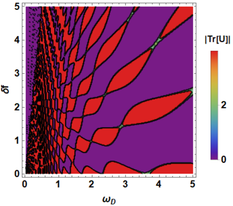
Figure 12: (Color online) Left Panel: Plot of the phase diagram showing $|{\rm Tr}U(T,0)|$ as a function of the amplitude $\delta f$ and frequency $\omega_{D}$ as obtained from second order FPT.

Next, we compute the second order term in the perturbative expansion of $U$

$$U^{\prime}_{2}(T,0) = (-i)^{2}\int_{0}^{T}dt_{1}\int_{0}^{t_{1}}dt_{2}U_{0}^{\dagger}(t_{1},0)H_{1}U_{0}(t_{1},0)$$ (87)

$$\times U_{0}^{\dagger}(t_{2},0)H_{1}U_{0}(t_{2},0)$$

Once again using the Pauli matrix dependence of $H_{1}$ and $U_{0}$ we find

$$U^{\prime}_{2} = -(\sigma_{+}\sigma_{-}I_{2}+\sigma_{-}\sigma_{+}I_{2}^{*})$$ (88)

$$I_{2} = \sum_{m,n}J_{m}(x)J_{n}(x)\int_{0}^{T}dt_{1}e^{i(m\omega_{D}+\delta f)t_{1}}$$

$$\times\int_{0}^{t_{1}}dt_{2}e^{i(n\omega_{D}+\delta f)t_{2}}$$

$$= \sum_{m,n}J_{m}(x)J_{n}(x)\frac{iT^{2}}{2(\pi m+\delta fT)}[-\delta_{mn}+\frac{e^{is}\sin s}{\pi n+\delta fT}]$$

where $x=2f_{0}/\omega_{D}$. The real and imaginary parts of $I_{2}$ can be read off as

$${\rm Re}[I_{2}] = \sum_{m,n}J_{m}(x)J_{n}(x)\frac{T^{2}}{2(\pi m+\delta fT)(\pi n+\delta fT)}\sin^{2}s$$

$${\rm Im}[I_{2}] = \beta=\sum_{m,n}J_{m}(x)J_{n}(x)\frac{T^{2}}{2(\pi m+\delta fT)}$$ (89)

$$\times[\delta_{mn}-\frac{\cos s\sin s}{(\pi n+\delta fT)}]$$

From Eq. 89 we note that $U_{2}-U_{1}^{2}/2$ depends only on ${\rm Im}[I_{2}]$. Thus to second order in perturbation theory, $U_{2}$ is given by

$$U_{2} = U_{0}(I+U^{\prime}_{1}+(U^{\prime}_{2}-U_{1}^{{}^{\prime}2}/2))=e^{-iH_{F}^{(2)}T}$$ (92)

$$= \left(\begin{array}[]{cc}e^{-is}(1+i\beta)&-i\alpha\sin y\\ i\alpha\sin y&e^{iy}(1-i\beta)\end{array}\right)$$

where $\alpha$ is defined in Eq. 9 in the main text. We unitarize $U_{2}$ following the same procedure as

$$H_{F}^{(2)} = \theta^{(2)}\left(n_{z}^{(2)}\sigma_{z}+in_{y}^{(2)}\sigma_{y}\right)/T$$

$$\sin(\theta^{(2)}T) = \sqrt{(\sin s-\beta\cos s)^{2}-\alpha^{2}\sin^{2}s}$$

$$n_{z}^{(2)}\sin(\theta^{(2)}T) = \sin s-\beta\cos s$$

$$n_{y}^{(2)}\sin(\theta^{(2)}T) = \alpha\sin s$$ (93)

The phase diagram is obtained from Eq. 93 by imposing condition on ${\rm Tr}[\exp[-iH_{F}^{(2)}T]]$ as discussed in the main text. This translates to the conditions $|\cos(\theta^{(2)})|>(<)2$ for the heating (non-heating) phases and $|\cos(\theta^{(2)})|=2$ on the transition line. The phase diagram, shown in Fig. 12 as a function of $\delta f$ and $\omega_{D}$ turns out to be qualitatively similar to that obtained using first order FPT (Fig. 1 in the main text).

Appendix B Mobius transformation

In this section, we discuss several aspects of the Mobius transformation corresponding to continuous protocol discussed in this work. To this end, we first relate to the Mobius transformation used in Ref. cft1, . It was shown that for an Hamiltonian $H=H_{0}+\tanh(\theta)(H_{+}+H_{-})/2$, the transformation is given by

$$z_{new}=\frac{[(1-\lambda)\cosh(2\theta)-(\lambda+1)]z+(\lambda-1)\sinh(2\theta)}{(1-\lambda)\sinh(2\theta)z+[(\lambda-1)\cosh(2\theta)-(\lambda+1)]}$$ (94)

where $\lambda=\exp[\delta\tau/\cosh(2\theta)]$ and $\tau$ is the imaginary time. We show below that this relation is reproduced for us at every Trotter steps.

To this end, we note that the instantaneous Hamiltonian at any time $\tau$ is of the form,

$$H=aH_{0}-\frac{b}{2}(H_{+}+H_{-})=a[H_{0}-\frac{b}{2a}(H_{+}+H_{-})]$$ (95)

where $a$ and $b$ depends on $\tau$. This indicates that for the non-heating phase one can write $\tanh 2\theta=b/a$ and $\lambda=\exp[a\delta\tau/\cosh(2\theta)]=\exp[\sqrt{a^{2}-b^{2}}\delta\tau]$, since $\cosh 2\theta=a/\sqrt{a^{2}-b^{2}}$ and $\sinh 2\theta=b/\sqrt{a^{2}-b^{2}}$. The Mobius transformation corresponding to such a Hamiltonian is given by

$$M_{1}=\begin{pmatrix}a_{1}&b_{1}\\ c_{1}&d_{1}\end{pmatrix}=\begin{pmatrix}s_{2}-s_{1}&\frac{b}{\sqrt{a^{2}-b^{2}}}(\exp[\sqrt{a^{2}-b^{2}}\delta\tau]-1)\\ -\frac{b}{\sqrt{a^{2}-b^{2}}}(\exp[\sqrt{a^{2}-b^{2}}\delta\tau]-1)&s_{2}+s_{1}\end{pmatrix}$$ (96)

where $s_{1}=(1-\exp[\sqrt{a^{2}-b^{2}}\delta\tau])a/\sqrt{a^{2}-b^{2}}$ and $s_{2}=(\exp[\sqrt{a^{2}-b^{2}}\delta\tau]+1)$. Thus we seek a matrix of the form $M=\frac{1}{2}(a\sigma_{z}-ib\sigma_{y})$ whose exponential gives the Mobius matrix $M_{1}$. Since

$$M_{2}=e^{-\Delta\tau M}=\left(\begin{array}[]{cc}\cosh\left(\frac{1}{2}\sqrt{a^{2}-b^{2}}\delta\tau\right)-\frac{a\sinh\left(\frac{1}{2}\sqrt{a^{2}-b^{2}}\delta\tau\right)}{\sqrt{(a-b)(a+b)}}&\frac{b\sinh\left(\frac{1}{2}\sqrt{a^{2}-b^{2}}\delta\tau\right)}{\sqrt{(a-b)(a+b)}}\\ -\frac{b\sinh\left(\frac{1}{2}\sqrt{a^{2}-b^{2}}\delta\tau\right)}{\sqrt{(a-b)(a+b)}}&\cosh\left(\frac{1}{2}\sqrt{a^{2}-b^{2}}\delta\tau\right)+\frac{a\sinh\left(\frac{1}{2}\sqrt{a^{2}-b^{2}}\delta\tau\right)}{\sqrt{(a-b)(a+b)}}\\ \end{array}\right)$$ (97)

we find $M_{2}(1,1)=a_{1}\exp[\frac{\delta\tau}{2}\sqrt{a^{2}-b^{2}}]$. Similar expressions can be seen for other elements $M_{2}$. Thus up to an overall irrelevant factor, our analysis reproduces the same Mobius at every Trotter step as in Ref. cft1, . A similar analysis can be easily carried out for the heating phase and leads to similar results.

Next, we show derive the form of $H_{F}$ using algebra of the Virasoro operators without resorting to their SU(1,1) representations. To this end, we begin from the time-dependent Hamiltonian given by Eq. 1. For $f_{0}\gg\delta f,1$, the zeroth order evolution operator is given by

$$U_{0}(t,0) = \exp\left[-iL_{0}\frac{2\pi t}{L}\left(\frac{f_{0}}{\omega_{D}t}\sin(\omega_{D}t)+\delta f\right)\right]$$ (98)

This leads to $U_{0}(T,0)=\exp[-2\pi isL_{0}/L]$ and $H_{F}(0)=2\pi sL_{0}/(LT)$; these results coincide with Eq. 15 for $L_{0}=\sigma_{z}/2$.

To obtain the next order correction to $U$, we write

$$U^{\prime}_{1}(T,0) = -i\int_{0}^{T}U_{0}^{\dagger}(t,0)\frac{\pi}{L}(L_{1}+L_{-1})U_{0}(t,0)dt$$

To evaluate this, we use the Baker-Campbell-Hausdorff relations for $L_{0}$ and $L_{\pm 1}$ which states

$$e^{iaL_{0}}(L_{1}+L_{-1})e^{-iaL_{0}} = e^{ia}L_{1}+e^{-ia}L_{-1}$$ (100)

Using Eq. 100 and identifying $a=-2\pi/L(f_{0}\sin(\omega_{D}t)/\omega_{D}+\delta ft)$ (Eq. 98), one can evaluate $U^{\prime}_{1}(T,0)$ in a straightforward manner. The integrals involved are similar to those in App. A and one obtains

$$U^{\prime}_{1}(T,0) = i\alpha\left[i(L_{1}+L_{-1})\sin s\right.$$ (101)

$$\left.+2\sin^{2}s/2(L_{1}-L_{-1})\right]$$

where $\alpha$ is given by Eq. 9 of the main text. Thus the expression of the evolution operator, up to first order in perturbation theory, is given by

$$U_{1}(T,0) = U_{0}(T,0)(I-U^{\prime}_{1}(T,0))$$

$$= e^{-i(2\pi s/L)TL_{0}}[I-i\alpha\{2\sin^{2}(s/2)(L_{1}-L_{-1})$$

$$+i\sin s(L_{1}+L_{-1})\}]$$

We note that this expression matches with Eq. 20 in the main text for $L_{0}=\sigma_{z}/2$ and $L_{\pm 1}=\mp\sigma{\pm}$.

Next we briefly comment on the unitarization procedure to be followed here. Since $U_{1}$ is non-unitary within first order FPT, we would like to unitarize it. This seems difficult without using the SU(1,1) representation of the Virasoro operators. Here we therefore concentrate on the high frequency regime, where the two routes to unitarization of $U_{1}$, discussed in the main text, leads to identical result. In the high frequency regime, $s\to 0$ and $\sin s/s\to 1$. Furthermore, in this regime once can write $U_{1}\simeq 1-iH_{F}T/\hbar$. Thus expanding Eq. B in powers of $s$ and retaining only first order terms, we find

$$H_{F}\simeq\frac{\theta}{T}[2n_{z}L_{0}+n_{y}(L_{1}+L_{-1})/i]$$ (103)

where $n_{z}$, $n_{y}$, and $\theta$ are given by Eq. 21 of the main text. We note that $H_{F}$ coincides with that obtained within first order FPT obtained in the main text with the identification $L_{0}=\sigma_{z}/2$ and $L_{1}+L_{-1}=i\sigma_{y}$ and is also consistent with the dynamic emergent symmetry discussed in the main text.

References

(1)
(2) J. Dziarmaga, Adv. Phys. 59, 1063 (2010); A. Dutta,
G. Aeppli, B. K. Chakrabarti, U. Divakaran, T.F. Rosenbaum, and D.
Sen, Quantum Phase Transitions in Transverse Field Spin Models:
From Statistical Physics to Quantum Information (Cambridge
University Press, Cambridge, 2015).
(3) A. Polkovnikov, K. Sengupta, A. Silva, and M. Vengalattore,
Rev. Mod. Phys. 83, 863 (2011); S. Mondal, D. Sen, and K.
Sengupta, Quantum Quenching, Annealing and Computation, edited
by Das, A., Chandra, A. & Chakrabarti, B. K. Lecture Notes in
Physics, Vol. 802 (Springer, Berlin, Heidelberg, 2010), Chap. 2, p.
21.
(4) L. D’Alessio and A. Polkovnikov, Ann. Phys.
333, 19 (2013).
(5) M. Bukov, L. D’Alessio, and A. Polkovnikov,
Adv. Phys. 64 139 (2015).
(6) M Heyl, A Polkovnikov, S Kehrein
Phys. Rev. Lett. 110, 135704 (2013); M. Heyl, Rep. Prog. Phys. 81,
054001 (2018).
(7) A. Sen, S. Nandy, K. Sengupta, Phys. Rev.
B 94, 214301 (2016); S. Nandy, K. Sengupta, and A. Sen, J.
Phys. A: Math. Theor. 51, 334002 (2018).
(8)A. Das, Phys.Rev. B 82, 172402 (2010); S Bhattacharyya, A Das,
and S Dasgupta, 86 054410 (2010); S. S. Hegde,H. Katiyar, T.
S. Mahesh, and A. Das, ibid. 90, 174407 (2014).
(9) S. Mondal, D. Pekker, and K. Sengupta, Europhys. Lett. 100, 60007 (2012);
U. Divakaran and K. Sengupta, Phys. Rev. B 90, 184303 (2014);
B. Mukherjee, A. Sen, D. Sen, and K. Sengupta, arXiv:2005.07715
(unpublished).
(10) B Mukherjee, S Nandy, A Sen, D Sen, and K Sengupta, Phys. Rev. B 101,
245107 (2020); B. Mukherjee, A. Sen, D. Sen, and K. Sengupta, Phys.
Rev. B 102, 014301 (2020).
(11) V Khemani, A Lazarides, R Moessner, and S. L. Sondhi, Phys. Rev. Lett. 116,
250401 (2016); N. Y. Yao, A. C. Potter, I.-D. Potirniche and A.
Vishwanath, Phys. Rev. Lett. 118 030401 (2017).
(12) J Zhang, PW Hess, A Kyprianidis, P Becker, A Lee, J Smith, G Pagano,
I-D Potirniche, A. C Potter, A Vishwanath, NY Yao, C Monroe Nature
543, 217 (2017).
(13) B Mukherjee, A Sen, D Sen, and K Sengupta, Phys. Rev. B 102, 075123
(2020).
(14) A Lazarides, A Das, and R. Moessner, Phys. Rev. E 90, 012110 (2014).
(15) I Bloch, J Dalibard, W Zwerger, Rev. Mod. Phys. 80, 885 (2008)
(16) M Greiner, O Mandel, T Esslinger, T.W. Hansch, and I Bloch
Nature 415 39 (2002);
(17) H Bernien, S Schwartz, A Keesling, H Levine, A Omran, H Pichler,
S Choi, A. S. Zibrov, M. Endres, M. Greiner, V. Vuletic, M. D. Lukin
Nature 551 579 (2017).
(18) S. N. Shevchenko, F. Ashhab, and F. Nori, Phys. Rep. 492, 1 (2010)
(19) M. Vogl, P. Laurell, A. D. Barr, and G. A. Fiete
Phys. Rev. X 9, 021037 (2019).
(20)A. Soori and D. Sen, Phys. Rev. B 82, 115432 (2010).
(21)T. Billitewsky and N. Cooper, Phys. Rev. A 91, 033601
(2015).
(22) R. Ghosh, B. Mukherjee, and K. Sengupta, Phys. Rev. B 102, 235114 (2020).
(23) C. C. Gerry and E. R. Vrscay, Phys. Rev. A 39,
5717 (1989).
(25)R. Fan, Y. Gu, A. Vishwanath and X. Wen, Phys. Rev. X 10,
031036 (2020); X. Wen, R. Fan, A. Vishwanath and Y. Gu,
arXiv:2006.10072 (unpublished).
(26)B. Lapierre, K. Choo, C. Tauber, A. Tiwari, T. Neupert and R.
Chitra, Phys. Rev. Research 2 (April, 2020); B. Lapierre, K.
Choo, A. Tiwari, C. Tauber, T. Neupert and R. Chitra, Phys. Rev.
Research 2 (September, 2020).
(27)B. Han and X. Wen, arXiv:2008.01123.
(28)M. Andersen, F. Norfjand and N. T. Zinner, arXiv:2011.08494.
(29) R. Fan, Y. Gui, A. Vishwanath, and X. Wen,
arXiv:2011.09491.
(30)H. Katsura, J. Phys. A:
Math. Theor. 44, 252001 (2011); I. Maruyama, H. Katsura, and
T. Hikihara, Phys. Rev. B 84, 165132 (2011); H. Katsura, J.
Phys. A: Math. Theor. 45, 115003 (2012); K. Okunishi,
arXiv:1603.09543.
(31) A. Milsted and G. Vidal, arXiv:1706.0143.
(32) There is a class of protocols for which exact
solutions to continually driven two state systems exists. However,
periodic drives do not fall in this category; see for example, G.
Dattolli, J. Gallardo, and A. Torre, Jour. Math. Phys. 27, 772
(1986).
(33) P. Di Franscesco, P. Mathieu, and D. Senechal, Conformal Field Theory, Springer-Verlag, New York (1997).
(34)A. A. Belavin, A. M. Polyakov and A. B. Zamolodchikov, Nuclear Physics B 241, 333 (1984).
(35)D. Poland, S. Rychkov, and A. Vichi, Rev. Mod. Phys.
91, 015002 (2019).
(36)T. Hartman, C. A. Keller and B. Stoica, JHEP 09, 118 (2014)
(37) V. Fateev and S. Ribault, JHEP 02, 001
(2012).
(38) E. Hijano, P. Kraus, E. Perlmutter and R. Snively,
JHEP 12, 077 (2015).
(39) T. Hartman, arXiv:1303.6955.
(40) E. Hijano, P. Kraus, E. Perlmutter and R. Snively,
JHEP bf 01, 146 (2016).
(41) P. Calabrese and J. Cardy, Journal of
Statistical Mechanics: Theory and Experiment 2004 P06002 (2004);
ibid., Journal of Statistical Mechanics: Theory and Experiment
2007 P10004 (2007); ibid, Journal of Statistical Mechanics:
Theory and Experiment 2016, P064003 (2016).