First phase space portrait of a hierarchical stellar structure in the Milky Way

Abstract

We present the first detailed observational picture of a possible ongoing massive cluster hierarchical assembly in the Galactic disk as revealed by the analysis of the stellar full phase-space (3D positions and kinematics and spectro-photometric properties) of an extended area ($6^{\circ}$ diameter) surrounding the well-known h and $\chi$ Persei double stellar cluster in the Perseus Arm. Gaia-EDR3 shows that the area is populated by seven co-moving clusters, three of which were previously unknown, and by an extended and quite massive ($M\sim 10^{5}M_{\odot}$) halo. All stars and clusters define a complex structure with evidence of possible mutual interactions in the form of intra-cluster over-densities and/or bridges. They share the same chemical abundances (half-solar metallicity) and age ($t\sim 20$ Myr) within a small confidence interval and the stellar density distribution of the surrounding diffuse stellar halo resembles that of a cluster-like stellar system. The combination of these evidences suggests that stars distributed within a few degrees from h and $\chi$ Persei are part of a common, sub-structured stellar complex that we named LISCA I. Comparison with results obtained through direct $N$-body simulations suggest that LISCA I may be at an intermediate stage of an ongoing cluster assembly that can eventually evolve in a relatively massive (a few $10^{5}M_{\odot}$) stellar system. We argue that such cluster formation mechanism may be quite efficient in the Milky Way and disk-like galaxies and, as a consequence, it has a relevant impact on our understanding of cluster formation efficiency as a function of the environment and redshift.

1 Introduction

It is widely accepted that most ($70-90\%$) stars in galaxies form in groups, clusters or hierarchies, and spend some time gravitationally bound with their siblings when still embedded in their progenitor molecular cloud (Lada & Lada, 2003; Portegies Zwart et al., 2010). Indeed, young stars tend to be grouped together into a hierarchy of scales where smaller and denser sub-regions (with a typical dimension of a few parsecs) are inside larger and looser ones (up to hundreds of parsecs; Elmegreen & Hunter 2010). The majority of such systems will be disrupted in their first few million years of existence, due to mechanisms possibly involving gas loss driven by stellar feedback (Moeckel & Bate, 2010) or encounters with giant molecular clouds (Gieles et al., 2006). Nonetheless, a fraction of proto-clusters will survive the embedded phase and remain bound over longer timescales. The process of clustered star formation has major implications for many fundamental astrophysical areas of research including the star formation process itself (McKee & Ostriker, 2007), the early interplay between stellar and gas dynamics and the consequences of gas expulsion for the cluster disruption (Baumgardt & Kroupa, 2007), the possible formation of gravitational wave sources (Di Carlo et al., 2019), and the dynamical properties of young star clusters (McMillan et al., 2007). Cluster formation has also key implications on our understanding of the assembly process of galaxies in a cosmological context. Indeed, major star-forming episodes in galaxies are typically accompanied by significant star cluster production (Forbes et al., 2018) and the main properties of these systems are thus strictly connected with those of their hosts (Brodie & Strader, 2006; Dalessandro et al., 2012). Indeed, massive star clusters may play a role in the formation of galactic sub-structures, and their partial or total dissolution contributes to the overall mass budget and stellar population properties of the hosts.

However, in order to efficiently exploit stellar clusters as tracers of galaxy and large-scale structure formation, it is essential to understand the physical processes setting their initial properties such as mass, structure and chemical composition and how they evolve across the cosmic time. In the last decade, many observational and theoretical studies have greatly enriched our understanding of the formation and early evolution of star clusters (e.g., Goodwin & Whitworth 2004; Allison et al. 2010; Parker et al. 2014; Adamo et al. 2015, 2020). However, questions concerning the possible presence of unifying principles governing the formation of different stellar systems are still unanswered (e.g., Bonnell et al. 2003; Longmore et al. 2014; Banerjee & Kroupa 2014, 2015, 2017; Kuhn et al. 2019, 2020). In addition, the presence in old globular clusters of multiple stellar populations characterized by specific abundance patterns in a number of light elements (see for example Bastian & Lardo 2018; Gratton et al. 2019 for recent reviews) has indeed raised new key questions on the physical mechanisms at the basis of clusters’ formation, and their dependence on the environment and the formation epoch (Krumholz et al., 2019). As a matter of fact, in spite of the tremendous observational and theoretical efforts our understanding of the star clusters’ formation history and the underlying physical processes is still in its infancy.

The unprecedented precision and sensitivity in measuring stellar parallaxes and proper motions secured by the Gaia mission (Gaia Collaboration et al., 2018, 2020) now provide key tools to study in detail nearby star-forming regions and to use them as ideal laboratories to shed new light on our understanding of cluster formation and early evolution. Indeed, several papers have been published recently on the subject (e.g. Beccari et al. 2018; Zari et al. 2018; Kuhn et al. 2019; Meingast et al. 2019; Lim et al. 2020).

In this context, in the present study, we focus on the neighborhood of the well-known young double clusters h and $\chi$ Persei (NGC 884 and NGC 869, respectively). This area is located in the Galactic Perseus Arm, which includes massive star-forming regions W3-W4-W5, with two giant H II regions (W4 and W5), a massive molecular ridge with active formation (W3), and several embedded star clusters and/or associations (Carpenter et al., 2000). The paper is organized as follows. The adopted data-set is presented in Sections 2, in Sections 3 and 4 the main spectro-photometric and kinematic properties of the area are described respectively. A comparison with a set of $N$-body simulations following the violent relaxation phase and its subsequent evolution is described in Section 5. The main conclusions are discussed in Section 6.

Figure 1: Panel a: Map of the Gaia sources (G$<$16) selected in proper motion and parallax as described in the text with respect to the position of the system barycenter (red cross). Blue arrows indicate the mean cluster motion in both the radial and tangential components with respect to the mean motion of the system. Light blue circles represent the positions of the SPA-TNG spectroscopic targets. Panel b: 2D surface density map obtained for the same stars as in the left panel. The blue contour levels span from 3 to $50\sigma$ with irregular steps.

2 The Perseus Arm complex under the Gaia and SPA-TNG lenses

For the present work we used photometric and astrometric information obtained from Gaia Early Data Release 3 (EDR3), we refer the reader to Gaia Collaboration et al. (2018, 2020) for details about the survey and available data. These data were complemented with high-resolution optical and near-infrared spectra obtained respectively with the HARPS-N (Cosentino et al., 2014) and the GIANO-B (Oliva et al., 2012; Tozzi et al., 2016) spectrographs mounted at the Italian Telescopio Nazionale Galileo (TNG) operated on the island of La Palma at the Spanish Observatorio del Roque de los Muchachos of the Instituto de Astrofisica de Canarias by the Fundacíon Galileo Galilei of the INAF (National Institute for Astrophysics). These observations are part of the TNG Large Program titled SPA - Stellar Population Astrophysics: the detailed, age-resolved chemistry of the Milky Way disk (Program ID A37TAC13, PI: L. Origlia), aimed at measuring detailed chemical abundances and radial velocities of the luminous stellar populations of the Milky Way (MW) thin disk and its associated star clusters (Origlia et al., 2019). Within SPA we collected HARPS-N spectra at $R\sim 115,000$ in the 378 - 691 nm range and GIANO-B spectra at $R\sim 50,000$ in the 950 - 2450 nm range for 37 stars among blue and red supergiants and young Main Sequence stars in the analysed area. HARPS-N spectra are automatically processed by the instrument data reduction software pipeline. GIANO-B spectra have been reduced using the GOFIO data reduction software code (Rainer et al., 2018).

2.1 Area characterization and cluster identification

We selected stars in the Gaia-EDR3 catalog, distributed within a circular projected area with radius of 3 degrees from h and $\chi$ Persei (Figure 1), located at $1\sigma$ from their mean distance ($d=2.353_{-0.197}^{+0.178}$ kpc, i.e. those stars having parallaxes in the range $0.385<\mu<0.465$ mas) and moving with similar mean velocities as the two clusters ($\mu_{\alpha}cos\delta=-0.64$ mas/yr and $\mu_{\delta}=1.17$ mas/yr) within a very strict tolerance range of $\pm 0.4$mas/yr, corresponding to about 4 km/s at their distance.

As shown in Figure 1a, in addition to h and $\chi$ Persei, other clusters, clumps and elongated structures are clearly visible in the area after applying the described proper motion and parallax selections. Two of them are the known open clusters NGC 957 and Basel 10. To identify the additional cluster-like components, we used the clustering algorithm DBSCAN (Density-Based Spatial Clustering of Applications with Noise). DBSCAN is a density-based clustering algorithm that interprets clusters as regions of high density separated by areas of low density in space, without requiring any additional prior. Only two parameters need to be set in the algorithm, which are $eps$ and $min_{samples}$. $eps$ defines the radius of neighborhood around a point x, and $min_{samples}$ represents the minimum number of neighbors within the $eps$ radius. Higher $min_{samples}$ or lower $eps$ values indicate higher densities necessary to identify a sub-system as a cluster. Inspecting Figure 1, it is quite evident that clusters in the considered region have different sizes and numbers of members, and therefore different densities. For this reason, the clustering analysis needs to be run more than once. We first focused on the central region, where h and $\chi$ Persei are located. We applied DBSCAN on a sub-sample of stars having magnitude G $<16$ and by imposing $min_{samples}$ = 45 and $eps=0.04$. This choice allowed us to isolate the main structures near the center of the map and to identify three main groups. Two of them are obviously h and $\chi$ Persei, the most dense and easy to identify, but a third component, very close to h Persei - that we will call hereafter N1 - has been also identified. Its location is highlighted in Figure 2. Then, we moved to the more external part, where less dense structures are present. We applied the DBSCAN algorithm only to such stars with the same magnitude cuts and using different parameters: $min_{samples}$ = 41 and $eps=0.06$ and we identified in this way four additional structures: the already known Basel 10 and NGC 957, and the two new additional systems that we name N 2 and N 3 (see Table 1 for a summary of the clusters’ main properties). We note that the identification of the new clusters is quite solid against different settings of the DBSCAN search. In particular, we checked that results do not vary when using different $eps$ values in the range 0.03-0.09.

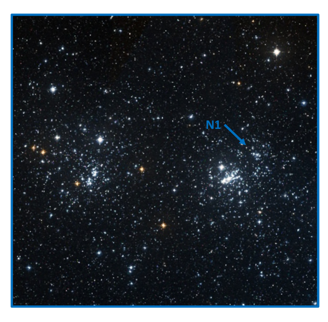
Figure 2: Zoomed view of the h and $\chi$ Persei region with highlighted the location of the newly identified system N1.

Table 1: Coordinates and mean velocities of the clusters identified in LISCA I

Cluster	RA(J2000)	Dec(J2000)	$\mu_{\alpha}cos(\delta)$	$\mu_{\delta}$ [mas/yr]	LOS-V
	(hh:mm:ss)	(dd:mm:ss)	[mas/yr]	[mas/yr]	(km/s)
$\chi$ Per	02:22:07.281	57:09:48.62	-0.621	-1.164	-45.3
$h$ Per	02:18:58.429	57:07:43.01	-0.662	-1.170	-45.6
NGC 957	02:33:23.532	57:33:17.32	-0.293	-1.120	-44.8
Basel 10	02:19:23.301	58:17:25.58	-0.466	-0.881	-53.0
N 1	02:18:23.612	57:12:40.79	-0.682	-1.165	-47.1
N 2	02:29:52.466	58:08:19.30	-0.433	-0.923	-49.7
N 3	02:28:44.542	57:41:37.94	-0.437	-0.957	-46.2

The presence of these additional clusters is remarkably evident in the two-dimensional (2D) density map shown in Figure 1b, which has been obtained by transforming the distribution of star positions into a smoothed surface density function through the use of a gaussian kernel with width of $3\arcmin$ (see for example Dalessandro et al. 2015). Interestingly, all star clusters in the complex show some degree of elongation, which is particularly relevant in the case of N 3. In addition, it is worth noting the presence of a significant overdensity bridging the regions between h and $\chi$ Persei and extending out to NGC 957 and N 2, which may be suggestive of ongoing tidal interactions or the remnants of primordial filamentary structures, which are now commonly found in the Milky Way disk (Kounkel & Covey, 2019). Figure 1b also shows the isodensity curves as obtained from 3 to 50 $\sigma$, where $\sigma$ is the ‘background’ density dispersion observed for stars located at about 3 degrees from h and $\chi$ Persei in the South-East quadrant. They clearly suggest the presence of a diffuse low-density stellar halo. The existence of a possible halo stellar distribution in the proximity of h and $\chi$ Persei (at distances $<0.5$ deg from the two clusters) was already proposed by Currie et al. (2010). Thanks to the Gaia astrometric information here we find that the halo actually extends with a rather irregular shape for at least 3 degrees from h and $\chi$ Persei at a $3\sigma$ significance level.

Are these co-moving clusters and diffuse halo (along with its sub-structures) part of a single system? Or are they just independent neighbors? The answers to these questions can have key implications on our understanding of their formation, evolution and, more in general, on stellar cluster formation and early dynamical processes. To address them we will examine two main lines of evidence that will be detailed in Sections 3 and 4.

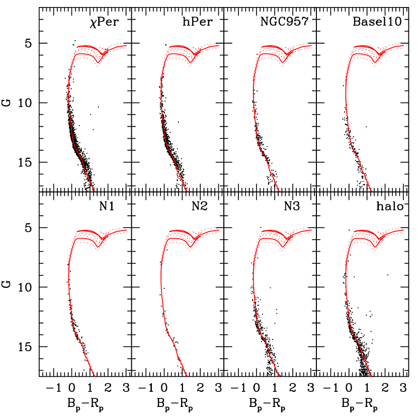
Figure 3: Gaia CMDs of the clusters detected around $h$ and $\chi$ Persei. The solid red line represents an isochrone (Bressan et al., 2012) of 20 Myr with metallicity [Fe/H]$=-0.29$, placed at a distance of 2.3 kpc and assuming $A_{v}=1.65$ mag. Dashed lines are isochrones at 15 Myr and 25 Myr. In general they reproduce reasonably well the h and $\chi$ Persei CMDs and they have been used as reference in the other panels.

3 Ages and chemical composition

We first derived stellar cluster and halo star chemical abundances by performing a detailed analysis of the high-resolution near-infrared spectra obtained with GIANO-B within the SPA-TNG Large Program. Chemical abundances and abundance patterns for all the most important metals are computed by using the MARCS model atmospheres (Gustafsson et al., 2008) and the spectral synthesis technique implemented in the Turbospectrum code (Alvarez & Plez, 1998; Plez, 2012) for the red supergiants in the sample. A detailed and comprehensive description of the analysis and results will be presented in a forthcoming paper (C. Fanelli et al. in preparation). For the purpose of this study we report that all the analyzed stars share the same metallicity within the uncertainties (which are typically of the order of 0.05 dex) with a mean value of [Fe/H]$=-0.29\pm 0.03$ dex and about solar-scaled [$\alpha$/Fe]. We compared these estimates with predictions from the Besançon Galaxy model (Robin et al., 2003) for stars in this region and selected in distance and proper motions as done before, and with results from surveys of the galactic disk (Mikolaitis et al., 2014; Hayden et al., 2014) at the galactocentric distance of h and $\chi$ Persei. The comparison distributions have a similar mean metallicity to that of stars analyzed here, but they are significantly broader extending for about 1.5 dex in the range $-1.0<[Fe/H]<0.3$ dex and thus suggesting that the lack of significant spread is not the expected outcome of the disk population properties in this area.

Secondly, we constrained cluster and halo ages by comparing the differential reddening corrected Gaia (G, Bp-Rp) color magnitude diagrams (CMDs) with a suitable set of isochrones (Figure 3). Extinction values have been assigned to each star in the Gaia catalog by interpolation with the Schlegel et al. (1998) extinction maps and corrected to estimates by Schlafly & Finkbeiner (2011). An accurate age derivation is certainly a challenge for young and scarcely populated clusters (in particular for N1, N2 and N3) as the turn-off region is significantly affected by low number counts (and relative fluctuations), stellar rotation and binarity (Li et al., 2019), which can make the adoption of a direct isochrone fitting approach unreliable. However, we stress that here we are mainly interested in investigating the presence of significant age differences among clusters. Currie et al. (2010) found that h, $\chi$ Persei and their surrounding stars are coeval with an age $t_{age}\sim 14$Myr. We extended such an analysis by using a set of PARSEC isochrones (Bressan et al., 2012). We adopted the derived mean metallicity ([Fe/H]=-0.29) and distance ($d=2.353$ kpc) and an average extinction value $A_{V}=1.65$ mag. We find that all systems are compatible with being almost coeval with ages in the 15-25 Myr range represented by the three isochrones shown in each CMD of Figure 3. While uncertainties on the distance can surely impact the derived ages, we stress that the main source of uncertainty is the limited number of bright stars needed to anchor the best-fit isochrone. Interestingly we find that also halo stars share the same age as clusters in agreement with previous findings (Currie et al., 2010). Only Basel 10 is possibly slightly older ($\sim 30$ Myr).

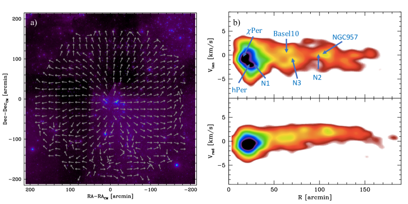
Figure 4: Panel a: Velocity map obtained for stars with G$<16$ superimposed to a Digital Sky Survey 2 false color image. A clear expansion signature is visible well resembling the expected behavior by Román-Zúñiga et al. (2019). The typical arrow size corresponds to a velocity of $\sim 1.5$ km/s. Panels b: radial and tangential velocities as a function of the distance from the system barycenter. The positions of the identified clusters are highlighted with blue arrows.

4 3D kinematical properties and structure

4.1 Kinematical properties

The mean motion of each star cluster in the plane of the sky has been obtained by using Gaia-EDR3 proper motions of stars within confidence radii in the range of $16.5\arcmin-25\arcmin$ from each clusters’ center (Table 1) and by adopting Equation (2) from Gaia Collaboration et al. (2018). Figure 1a shows the derived cluster velocity vectors with respect to the entire system mean motion. All velocities were corrected for the effects of perspective expansion/contraction by using the procedures described in van de Ven et al. (2006), which however, result to be negligible (of the order of few cents of km/s) with respect to the typical stellar motions. By construction, all clusters’ average motions reciprocally coincide within $\sim 3$ km/s in the sky component of the velocity vector. We then split the entire system in a $20\times 20$ regular cell grid with each cell having a side of $16.5\arcmin$ and including only stars with G$<16$. In each cell, we derived the average motions of stars with respect to the entire system mean motion. Also in this case, we properly accounted for the effects of perspective expansion/contraction. The resulting velocity map is shown in Figure 4a, where an almost regular expansion pattern is clearly visible. Such a kinematical behavior might be due to a combination of effects associated with the dynamics of the violent relaxation phase and the dynamical response of the cluster to the mass loss from supernovae explosions and gas expulsion, all of which can cause a significant cluster radial expansion. Indeed, a significant fraction of nearby young ($t<5$ Myr) clusters and associations has been recently found to show a similar behavior based on Gaia DR2 data (Kuhn et al., 2019). We stress here that the expansion of a stellar system is a transient process not associated to a single evolutionary path and eventual fate. We further discuss this point in Section 4.2. We also note that in the specific case of the analyzed region this behavior can be in part linked to the so-called “Hubble Flow-like” large scale motion that affects regions extending for several tens of degrees in the Perseus Arm and which has been observed (Román-Zúñiga et al., 2019) to be moving the Perseus Arm away from the W3-W4-W5 massive star formation zones with a velocity of 15 km/s/kpc.

The panels in Figure 4b show the smoothed density distributions of both the radial and tangential velocities as a function of the distance from the system barycenter. The radial component shows a quite narrow distribution slowly increasing as a function of the distance and reaching a peak of $\sim 2$ km/s at $R\sim 100\arcmin$, thus confirming the expansion signal. The tangential velocity component shows a broader distribution, with a slowly declining trend as a function of the distance that can be indicative of a possible large scale (of the order of some degrees) rotation pattern with amplitude of $2-3$ km/s (corresponding to about $0.2-0.3$ mas/yr).

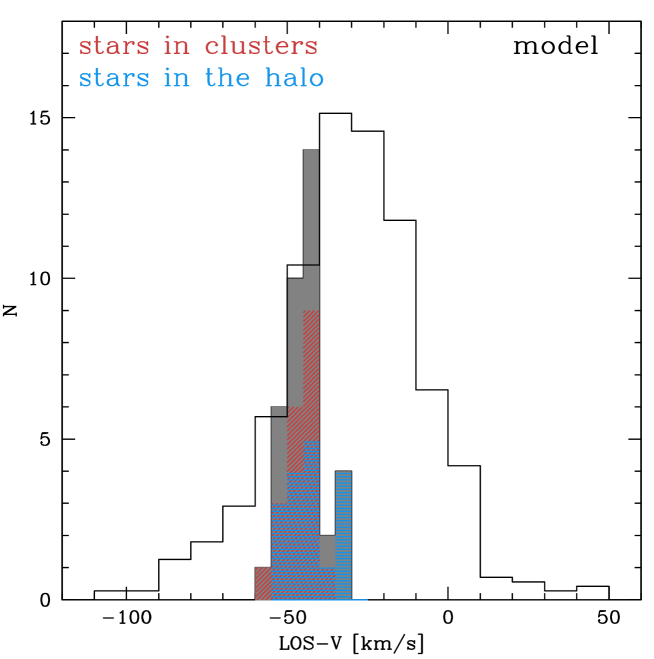
Figure 5: Line of sight velocity distribution of the entire sample of stars observed in LISCA I by using HARPS-TNG as part of the SPA-TNG Large Program. In red is the velocity distribution of stars associated with clusters (see the main text for the selection details) and in blue the distribution of the stars associated with the halo. The grey histogram represents the LOS-V distribution of all the analyzed stars and the black one represents the result of the Besançon model.

To check for the line-of-sight velocity (LOS-V) distribution, we complemented Gaia proper motions with LOS-Vs obtained with HARPS-N within the SPA-TNG Large Program for the 37 bright stars fulfilling the proper motions and parallax selection criteria described before (light blue symbols in Figure 1a; see Section 3). Accurate (at better than 1 km/s) heliocentric radial velocities for the observed stars have been obtained by means of standard cross-correlation technique (Tonry & Davis, 1979) as implemented in the IRAF (Tody, 1986) task FXCOR and suitable synthetic templates computed with the SYNTHE code (Kurucz, 1973). The median line-of-sight velocity of all the analyzed stars is $(-43.9\pm 3.5)$ km/s.

The resulting LOS-V distribution of cluster and halo stars is shown in Figure 5. For each cluster, we obtained the mean velocity by averaging out the LOS-Vs of stars falling within $16.5\arcmin-25\arcmin$ from the clusters’ center. Our analysis shows that the clusters are moving at an average LOS-V${}_{clusters}\sim-47.4$ km/s with $\sigma\sim 2.9$ km/s. The stars (17) not directly associable with clusters are here tentatively assigned to the halo. The agreement between the line-of-sight motion of such stars and that of the cluster is satisfactory, as shown in Figure 5, with an average velocity LOS-V${}_{halo}\sim-43.4$ km/s and $\sigma\sim 6.3$ km/s. Figure 5 also shows a comparison with the LOS-V distribution obtained from the Besançon model for the same sample of stars used before. The observed LOS-V distribution is significantly narrower than the one expected for field disk stars within the same field of view, thus making it unlikely to be just a random extraction of disk star velocities in the area.

4.2 Mass and structural properties

A detailed characterization of the individual clusters in the region will be the subject of a related paper (E. Dalessandro, in prep.). Here we provide further details on the diffuse stellar halo. To determine the projected density profile of the halo we used stars with G$<16$ and selected in proper motions and parallaxes as described before. We also subtracted the contribution of each cluster by removing all stars located at a distance $r<25\arcmin$ from each cluster center. We divided the field of view in 16 concentric annuli centered on the system center and split in a number (from 2 to 4 depending on the azimuthal coverage) of sub-sectors. We then counted the number of stars lying within each sub-sector and divided it by the sub-sector area. The stellar density in each annulus was finally obtained as the average of the sub-sector densities, and the standard deviation among the sub-sectors densities was adopted as error. The resulting density profile is shown in Figure 6. The background corrected profile is characterized by a typical profile with a high-density core and low-density halo that can be well fit by a single-mass King model (King, 1966) thus suggesting that the diffuse stellar halo resembles a low-density cluster-like stellar structure. To determine the physical parameters of the halo we used single-mass, spherical and isotropic King models (King 1966). This is a single-parameter family, where the shape of the density profile is uniquely determined by the dimensionless parameter W₀ (or concentration c). To determine the best-fit model we compared the background-subtracted surface density profile with the King model family, and found the halo profile to be best-fit by a low-density model ($c=0.84$) with large core and half-mass radii $r_{c}=1770.0^{+182.4}_{-194.7}\arcsec$ and $R_{h}=3381.1^{+287.1}_{-304.5}\arcsec$.

We analyzed the mass function (MF) of the likely halo stars. Stellar masses were derived by interpolation as a function of the G-band magnitude with the 20 Myr isochrone used in Figure 3. Starting from the observed MF we derived the stellar mass of the entire system. We normalized both a Salpeter Salpeter (1955) and a Kroupa (Kroupa, 2001) theoretical initial mass functions (IMFs) to the high-mass portion (roughly corresponding to G$<12$) of the observed MF, where the photometric completeness of Gaia is expected to be close to $100\%$ in relatively low-density environments like those surrounding h and $\chi$ Persei. Then, the total mass is simply given by the integral of the normalized IMF in the mass range $(0.1<m<8)M_{\odot}$. We find that the total mass ranges from $M_{tot}\sim 6\times 10^{5}M_{\odot}$ when a Salpeter IMF is adopted to $1.5\times 10^{5}M_{\odot}$ when a Kroupa IMF is used instead, making it compatible with the mass regime of the so called Young Massive Clusters (YMCs) and with the peak of the present-day mass distribution of Galactic globular clusters. We find that the mass is equally split between clusters and the diffuse stellar halo. Stellar clusters have masses ranging from $\sim 2\times 10^{4}M_{\odot}$ as for $\it h$ and $\chi$ Persei (in quite good agreement with estimates from Currie et al. 2010) and $\sim 500M_{\odot}$ for N3. By adopting the same heliocentric distance as before and a galactocentric distance of 9.7 kpc, we find that the formal Jacobi radius of the system (which gives an approximate indication of the expected possible extension of the system), ranges from $\sim 140\arcmin$ to $\sim 200\arcmin$ (corresponding to 91-132 pc) depending on the adopted mass, thus nicely matching the observed properties of the analyzed structure.

We emphasize that the observed radial variation of the LISCA I halo is not expected for a generic sample of field stars. The radial profile we found thus provide further evidence that the halo identified in our analysis is one of the dynamical components of the complex cluster structure.

In addition, by combining all the structural and kinematic information collected so far we can calculate both the one dimensional 1D ($\sigma_{1D}$) and the virial velocity dispersions ($\sigma_{vir}^{2}=GM/\eta R_{h}$, see e.g. equation 19 in Kuhn et al. 2019), where $\sigma_{vir}$ represents the velocity dispersion of a virialized stellar system. Kuhn et al. (2019) used these two quantities for an approximate determination of the dynamical state of 28 young (1-5 Myr) nearby clusters. Following Kuhn et al. (2019), we have adopted $\eta\sim 10$ as appropriate for a stellar system with a Plummer star density distribution. We find that $\sigma_{1D}=1.54\pm 0.06$ km/s and $\sigma_{vir}$ ranges from $1.29$ km/s and $2.63$ km/s for $R_{h}=3381.1\arcsec$ and assuming a total mass in the $1.5-6\times 10^{5}M_{\odot}$ range. While these values provide only an approximate description of the system’s dynamical state, they suggest it should be gravitationally bound.

The purely observational results collected so far show that a) all stars and clusters distributed close to h and $\chi$ Persei define a quite complex structure with evidence of possible mutual interactions in the form of intra-cluster over-densities and/or bridges, b) they have the same metallicity, $\alpha$-element abundance and age within a small interval, c) the stellar density distribution of the surrounding diffuse stellar halo resembles that of a cluster-like stellar system. The combination of these evidences clearly suggests that stars distributed within a few degrees from h and $\chi$ Persei are part of a common, sub-structured and recently formed/still forming stellar system that we name hereafter LISCA I.

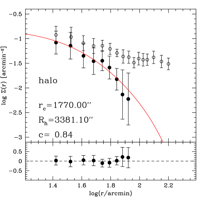
Figure 6: Density profile of the diffuse stellar halo obtained within the selected field of view by subtracting the contribution of clusters as described in the text. Open circles represent the observed density, while the black ones are the background subtracted density values. In red, the best fit mono-mass King model is super-imposed to the observed values.

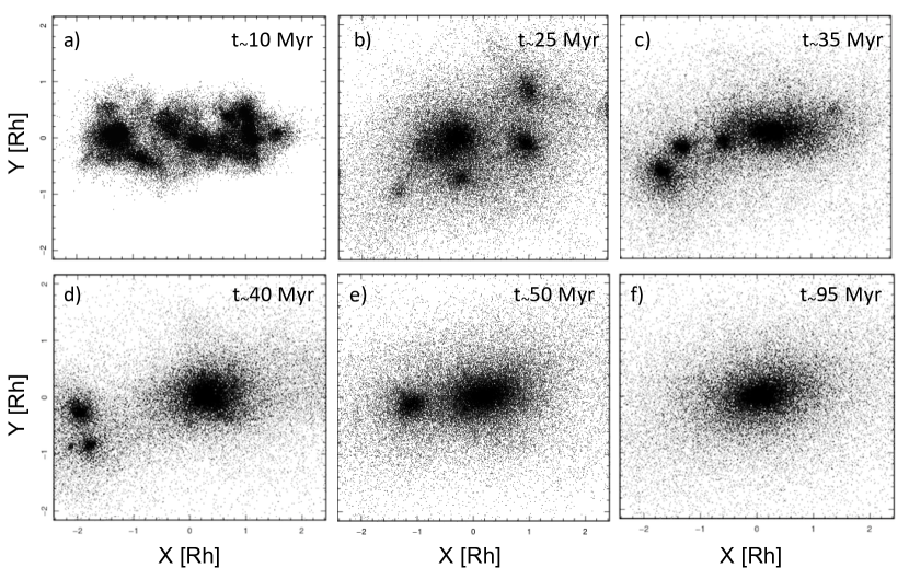
Figure 7: Schematic view of a hierarchical cluster formation path as traced by the $N$-body simulations presented in this work. The axis are expressed in unit of the system Rh.

5 N-body simulations of a LISCA I - like system

Several theoretical studies have explored the early dynamical evolution of star clusters and tried to establish a connection between the initial structural and kinematical properties of molecular clouds to the formation of single and multiple stellar clusters (see for example Goodwin & Whitworth 2004; Allison et al. 2010; Parker et al. 2014; Banerjee & Kroupa 2014, 2015; Fujii & Portegies Zwart 2016; Arnold et al. 2017; Sills et al. 2018). In order to provide an example of the evolutionary history behind a system with structural and kinematical properties similar to those found in LISCA I, we show here the results of one of the realisations of a large suite of direct $N$-body simulations aimed at investigating the violent relaxation phase of a cluster, starting from initial conditions characterized by non-vanishing total angular momentum and a fractal density distribution, to heuristically represent a turbulent giant molecular cloud in a variety of kinematic and structural initial states.

While a comprehensive description and phase space analysis of this suite of $N$-body simulations along with a comparison with previous works will be presented in a separate article (A.L. Varri et al., in preparation), here we provide a short summary of the key properties of the survey. The initial conditions for these simulations were generated by using McLuster (Kuepper et al., 2011), with both homogeneous and inhomogeneous mass distributions. The values of the fractal dimension explored in the survey range from 1.6 to 3.0, with D=3.0 corresponding to a homogeneous stellar system. As for the stellar velocities, the systems have been initialized with a variety of “temperatures” of the stellar distribution, with a ratio of the kinetic energy due to random stellar motions to the potential energy of the system ranging from 0.1 (‘cold’) to 0.25 (‘warm’). With these initial conditions, the system is typically initially out of virial equilibrium, undergoes the so-called violent relaxation process (Aarseth et al., 1988), and eventually settles into an equilibrium configuration in a few dynamical times. Such a process naturally produces a characteristic pressure anisotropy signature (van Albada, 1982; Trenti et al., 2005; Vesperini et al., 2014) in the velocity space of the resulting configuration. In addition, we have also explored the effects of the presence of some primordial angular momentum (Gott, 1973; Boily et al., 1999). Internal rotation was added to the initial conditions such that the ratio between the kinetic energy due to ordered motions and the potential energy could assume a range of values from 0.0 (non-rotating) to 0.5 (moderately rotating), and the initial rotation curve is always approximately solid-body. All $N$-body simulations have N=65536 equal-mass particles and the simulations have been performed with the direct summation code Starlab (Portegies Zwart et al., 2001). The initial mass distribution of the simulation depicted in Figure 7 is characterized by a value of the fractal dimension parameter D=2.4. Such a definition corresponds to significant deviations from a uniform spatial distribution of stellar positions. The initial kinematic state is ‘cold’ (random kinetic energy/potential energy = 0.1) and moderately rotating (ordered kinetic energy/potential energy =0.5).

A representative example of the early dynamical evolution explored in such $N$-body simulations is illustrated in Figure 7 and can be summarized as follows: a) at early stages the distribution of stars preserves the initial inhomogeneities and tens of small clumps ($\sim 100M_{\odot}$) can be identified (Figure 7a). Several of these clumps are then destroyed because of dynamical interactions and some of their stars contribute to the surrounding field and to the formation of a gravitationally bound halo (Figures 7b,c); b) At later time, the surviving clumps merge to form a few more massive ($10^{3}-10^{4}M_{\odot}$) and larger clusters (Figure 7d,e); c) Finally, one or two clusters survive this hierarchical merger process and will eventually evolve into a single massive cluster (Figure 7f).

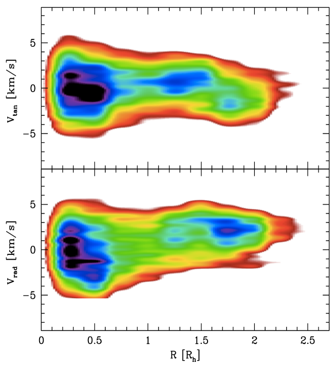
Figure 8: Radial and tangential velocity distributions for the simulation snapshot corresponding to Figure 7c.

We emphasize that the snapshots shown here are not meant to provide a dynamical model tailored to the evolution of the LISCA I system, but just to illustrate the typical dynamical evolution of a hierarchical cluster assembly process in the presence of a realistic degree of kinematic complexity. Such complexity, which is often neglected in star cluster formation studies, has a key role in determining the properties of the violent relaxation phase, the longevity of the population of sub-clumps, and the structural and kinematic properties of the resulting end-product massive cluster. The six snapshots in Figure 7 show the system after about 1.4, 3.0, 4.6, 5.4, 6.7, and 12.6 free-fall timescales ($t_{ff}$). Assuming an initial mass of $M_{i}\sim 6\times 10^{5}M_{\odot}$ and a 3D half-mass radius $r_{h}\sim 40$pc, the snapshot in Figure 7b would represent the structure of the system at the approximate age of the LISCA I system ($20-25$ Myr). Therefore, the observational properties of h and $\chi$ Persei and their surrounding structures, fit well within an early stage of the hierarchical cluster assembly process (Figures 7b,c), which may potentially lead the system to the formation of a stellar system of some $10^{5}M_{\odot}$ within a short timescale ($\sim 100$ Myr – Figure 7f).

Also, the kinematical patterns corresponding to the early snapshots of Figure 7 (see Figure 8) nicely resemble those observed in LISCA I. In particular, we note that also the expansion pattern observed in LISCA I is compatible with the results from our suite of simulations and shown in the lower panel of Figure 8 to compare with Figure 4b. As discussed in Section 4.1, although there might be different physical mechanisms responsible for the expansion of the system, the (qualitative) agreement with the simulations suggests that it is compatible with the dynamical evolution of a system in the early phases of a hierarchical cluster assembly.

Finally we point out that although our simulations explore the evolution of systems starting with a clumpy mass distribution similar to one that could arise from a hierarchical star formation process, structural properties like those observed in the current dynamical phase of LISCA I could also result from the growth of density fluctuations in a system emerging with a more homogeneous initial mass distribution from a monolithic formation event (see e.g. Aarseth et al. 1988).

6 Summary and Conclusions

The results presented in this paper suggest that we might have caught in the act, for the first time in our “courtyard”, an ongoing hierarchical cluster assembly process for which the structural and kinematical properties of the involved components are described in detail.

It is hard to make strong predictions about the final by-product of LISCA I and the fraction of mass that will be actually retained during its evolution, as it may depend on many factors including the nature and duration of the observed expansion. However, the results obtained here suggest that the formation of small stellar structures and their subsequent growth driven by dynamical interactions might have strongly contributed to shape the observed properties of LISCA I, thus possibly representing a viable process to form massive and long-lived stellar systems also in relatively low-density environments. This mechanism was long believed to work only in massive starburst galaxies, such as M83 (Bastian et al., 2011) and M51 (Chandar et al., 2011), but to be inefficient in local, lower density disk galaxies such as the Milky Way or M31 (Krumholz et al., 2012).

In case LISCA I will be able to continue its evolution as schematically shown in Figure 7, it can produce a YMC or alternatively, given its extension ($R_{h}\sim 35$pc), it could also be identified as the progenitor of a so-called diffuse star cluster (also known as “faint fuzzy”; Larsen & Brodie 2000), that is characterized by a mass comparable to that of globular clusters while being significantly more extended. These systems have a strongly debated origin (Fellhauer & Kroupa, 2002), they are observed in external galaxies (Huxor et al., 2005), but have remained elusive in the Milky Way so far. In any case, these results may give a boost to the possibility of studying massive cluster formation by resolving individual stars in our neighborhood thus constraining the physical mechanisms with a level of detail that cannot be achieved for distant systems. Interestingly in this respect, the properties of the interstellar medium in the Galactic disk are similar to those in the disks of other nearby galaxies (Longmore et al., 2013). As a consequence, our understanding of star formation and feedback in close young clusters and associations can probe star formation across much of the local Universe.

Recent results obtained by Gaia (Cantat-Gaudin et al., 2018; Castro-Ginard et al., 2018) have shown that the Galactic disk structure is composed by large numbers of stellar groups, hierarchies, young clusters with most of them being distributed along filamentary, string-like structures with similar properties to those observed in the Perseus Arm and in the LISCA I (see for example Kuhn et al. 2019). This opens the possibility to check whether the hierarchical assembly process framed here can be efficient within disk-like galaxies such as the Milky Way. Our study would therefore introduce a possible new picture in which the different appearance and properties of young stellar aggregates from clumps and filaments as observed in the Galaxy spiral arms (e.g. Kounkel & Covey 2019; Kuhn et al. 2019), to double/multiple clusters as found in the Magellanic Cloud disks (e.g. Dieball et al. 2002; Mucciarelli et al. 2012; Dalessandro et al. 2018) and finally to massive globulars, can be interpreted as the morphological evidence of different evolutionary phases of the same hierarchical assembly process. This has important implications on our understanding of the environmental conditions (both locally and in the distant Universe) necessary to form massive stellar clusters and, as consequence, on the evolution of stellar cluster properties over cosmic time. In this respect, it is extremely interesting to note that the hierarchical build-up of massive stellar clusters may play an important role during the formation of the multiple stellar populations observed in old GCs and could be one of the key ingredients necessary to explain the variety of stellar populations’ properties (Bekki, 2017; Bailin, 2018; Howard et al., 2019). Finally, the results obtained for LISCA I and the $N$-body simulations also show that the kinematic state of the initial molecular cloud play a key role in prolonging the survival timescales of sparse and low-mass clumps and associations, thus mitigating the discrepancy between their observed and expected numbers in the Galaxy and providing further support to a primordial origin of the ‘kinematic complexity’ currently emerging in old GCs (Lanzoni et al., 2018; Kamann et al., 2018).

References

- Aarseth et al. (1988) Aarseth, S. J., Lin, D. N. C., & Papaloizou, J. C. B. 1988, ApJ, 324, 288
- Adamo et al. (2015) Adamo, A., Kruijssen, J. M. D., Bastian, N., et al. 2015, MNRAS, 452, 246
- Adamo et al. (2020) Adamo, A., Hollyhead, K., Messa, M., et al. 2020, MNRAS, doi:10.1093/mnras/staa2380
- Allison et al. (2010) Allison, R. J., Goodwin, S. P., Parker, R. J., et al. 2010, MNRAS, 407, 1098
- Alvarez & Plez (1998) Alvarez, R. & Plez, B. 1998, A&A, 330, 1109
- Arnold et al. (2017) Arnold, B., Goodwin, S. P., Griffiths, D. W., et al. 2017, MNRAS, 471, 2498
- Banerjee & Kroupa (2014) Banerjee, S. & Kroupa, P. 2014, ApJ, 787, 158
- Banerjee & Kroupa (2015) Banerjee, S. & Kroupa, P. 2015, MNRAS, 447, 728
- Banerjee & Kroupa (2017) Banerjee, S. & Kroupa, P. 2017, A&A, 597, A28
- Banerjee & Kroupa (2018) Banerjee, S. & Kroupa, P. 2018, The Birth of Star Clusters, 143
- Baumgardt & Kroupa (2007) Baumgardt, H. & Kroupa, P. 2007, MNRAS, 380, 1589
- Bailin (2018) Bailin, J. 2018, ApJ, 863, 99
- Bastian et al. (2011) Bastian, N., Adamo, A., Gieles, M., et al. 2011, MNRAS, 417, L6
- Bastian & Lardo (2018) Bastian, N. & Lardo, C. 2018, ARA&A, 56, 83
- Beccari et al. (2018) Beccari, G., Boffin, H. M. J., Jerabkova, T., et al. 2018, MNRAS, 481, L11. doi:10.1093/mnrasl/sly144
- Bekki (2017) Bekki, K. 2017, MNRAS, 469, 2933
- Boily et al. (1999) Boily, C. M., Clarke, C. J., & Murray, S. D. 1999, MNRAS, 302, 399
- Bonnell et al. (2003) Bonnell, I. A., Bate, M. R., & Vine, S. G. 2003, MNRAS, 343, 413
- Bressan et al. (2012) Bressan, A., Marigo, P., Girardi, L., et al. 2012, MNRAS, 427, 127
- Brodie & Strader (2006) Brodie, J. P. & Strader, J. 2006, ARA&A, 44, 193
- Cantat-Gaudin et al. (2018) Cantat-Gaudin, T., Jordi, C., Vallenari, A., et al. 2018, A&A, 618, A93
- Carpenter et al. (2000) Carpenter, J. M., Heyer, M. H., & Snell, R. L. 2000, ApJS, 130, 381
- Castro-Ginard et al. (2018) Castro-Ginard, A., Jordi, C., Luri, X., et al. 2018, A&A, 618, A59
- Chandar et al. (2011) Chandar, R., Whitmore, B. C., Calzetti, D., et al. 2011, ApJ, 727, 88
- Cosentino et al. (2014) Cosentino, R., Lovis, C., Pepe, F., et al. 2014, Proc. SPIE, 9147, 91478C
- Currie et al. (2010) Currie, T., Hernandez, J., Irwin, J., et al. 2010, ApJS, 186, 191
- Dalessandro et al. (2012) Dalessandro, E., Schiavon, R. P., Rood, R. T., et al. 2012, AJ, 144, 126
- Dalessandro et al. (2015) Dalessandro, E., Miocchi, P., Carraro, G., et al. 2015, MNRAS, 449, 1811
- Dalessandro et al. (2018) Dalessandro, E., Zocchi, A., Varri, A. L., et al. 2018, MNRAS, 474, 2277. doi:10.1093/mnras/stx2892
- Di Carlo et al. (2019) Di Carlo, U. N., Giacobbo, N., Mapelli, M., et al. 2019, MNRAS, 487, 2947
- Dieball et al. (2002) Dieball, A., Müller, H., & Grebel, E. K. 2002, A&A, 391, 547. doi:10.1051/0004-6361:20020815
- Elmegreen & Hunter (2010) Elmegreen, B. G. & Hunter, D. A. 2010, ApJ, 712, 604
- Fellhauer & Kroupa (2002) Fellhauer, M. & Kroupa, P. 2002, AJ, 124, 2006
- Forbes et al. (2018) Forbes, D. A., Bastian, N., Gieles, M., et al. 2018, Proceedings of the Royal Society of London Series A, 474, 20170616
- Fujii & Portegies Zwart (2016) Fujii, M. S. & Portegies Zwart, S. 2016, ApJ, 817, 4
- Gaia Collaboration et al. (2018) Gaia Collaboration, Brown, A. G. A., Vallenari, A., et al. 2018, A&A, 616, A1
- Gaia Collaboration et al. (2020) Gaia Collaboration, Brown, A. G. A., Vallenari, A., et al. 2020, arXiv:2012.01533
- Gieles et al. (2006) Gieles, M., Portegies Zwart, S. F., Baumgardt, H., et al. 2006, MNRAS, 371, 793
- Gieles & Portegies Zwart (2011) Gieles, M. & Portegies Zwart, S. F. 2011, MNRAS, 410, L6
- Goodwin & Whitworth (2004) Goodwin, S. P. & Whitworth, A. P. 2004, A&A, 413, 929
- Gott (1973) Gott, R. J. 1973, ApJ, 186, 481
- Gratton et al. (2019) Gratton, R., Bragaglia, A., Carretta, E., et al. 2019, A&A Rev., 27, 8
- Gustafsson et al. (2008) Gustafsson, B., Edvardsson, B., Eriksson, K., et al. 2008, A&A, 486, 951
- Hayden et al. (2014) Hayden, M. R., Holtzman, J. A., Bovy, J., et al. 2014, AJ, 147, 116
- Helmi et al. (2018) Helmi, A., Babusiaux, C., Koppelman, H. H., et al. 2018, Nature, 563, 85
- Howard et al. (2019) Howard, C. S., Pudritz, R. E., Sills, A., et al. 2019, MNRAS, 486, 1146
- Huxor et al. (2005) Huxor, A. P., Tanvir, N. R., Irwin, M. J., et al. 2005, MNRAS, 360, 1007
- Kamann et al. (2018) Kamann, S., Husser, T.-O., Dreizler, S., et al. 2018, MNRAS, 473, 5591
- King (1966) King, I. R. 1966, AJ, 71, 64
- Kounkel & Covey (2019) Kounkel, M. & Covey, K. 2019, AJ, 158, 122
- Kroupa (2001) Kroupa, P. 2001, MNRAS, 322, 231
- Krumholz et al. (2012) Krumholz, M. R., Dekel, A., & McKee, C. F. 2012, ApJ, 745, 69
- Krumholz et al. (2019) Krumholz, M. R., McKee, C. F., & Bland-Hawthorn, J. 2019, ARA&A, 57, 227
- Kuepper et al. (2011) Kuepper, A. H. W., Maschberger, T., Kroupa, P., et al. 2011, Astrophysics Source Code Library
- Kuhn et al. (2019) Kuhn, M. A., Hillenbrand, L. A., Sills, A., et al. 2019, ApJ, 870, 32
- Kuhn et al. (2020) Kuhn, M. A., Hillenbrand, L. A., Carpenter, J. M., et al. 2020, ApJ,
- Kurucz (1973) Kurucz, R. L. 1973, Ph.D. Thesis
- Lada & Lada (2003) Lada, C. J. & Lada, E. A. 2003, ARA&A, 41, 57
- Lanzoni et al. (2018) Lanzoni, B., Ferraro, F. R., Mucciarelli, A., et al. 2018, ApJ, 861, 16
- Larsen & Brodie (2000) Larsen, S. S. & Brodie, J. P. 2000, AJ, 120, 2938
- Li et al. (2019) Li, C., Sun, W., de Grijs, R., et al. 2019, ApJ, 876, 65
- Lim et al. (2020) Lim, B., Hong, J., Yun, H.-S., et al. 2020, ApJ, 899, 121. doi:10.3847/1538-4357/aba0a3
- Longmore et al. (2013) Longmore, S. N., Bally, J., Testi, L., et al. 2013, MNRAS, 429, 987
- Longmore et al. (2014) Longmore, S. N., Kruijssen, J. M. D., Bastian, N., et al. 2014, Protostars and Planets VI, 291
- McKee & Ostriker (2007) McKee, C. F. & Ostriker, E. C. 2007, ARA&A, 45, 565
- McMillan et al. (2007) McMillan, S. L. W., Vesperini, E., & Portegies Zwart, S. F. 2007, ApJ, 655, L45
- Meingast et al. (2019) Meingast, S., Alves, J., & Fürnkranz, V. 2019, A&A, 622, L13. doi:10.1051/0004-6361/201834950
- Mikolaitis et al. (2014) Mikolaitis, Š., Hill, V., Recio-Blanco, A., et al. 2014, A&A, 572, A33
- Moeckel & Bate (2010) Moeckel, N. & Bate, M. R. 2010, MNRAS, 404, 721
- Mucciarelli et al. (2012) Mucciarelli, A., Origlia, L., Ferraro, F. R., et al. 2012, ApJ, 746, L19. doi:10.1088/2041-8205/746/2/L19
- Oliva et al. (2012) Oliva, E., Origlia, L., Maiolino, R., et al. 2012, Proc. SPIE, 8446, 84463T
- Origlia et al. (2019) Origlia, L., Dalessandro, E., Sanna, N., et al. 2019, A&A, 629, A117
- Parker et al. (2014) Parker, R. J., Wright, N. J., Goodwin, S. P., et al. 2014, MNRAS, 438, 620
- Plez (2012) Plez, B. 2012, Astrophysics Source Code Library
- Portegies Zwart et al. (2001) Portegies Zwart, S. F., McMillan, S. L. W., Hut, P., et al. 2001, The Influence of Binaries on Stellar Population Studies, 371
- Portegies Zwart et al. (2010) Portegies Zwart, S. F., McMillan, S. L. W., & Gieles, M. 2010, ARA&A, 48, 431
- Rainer et al. (2018) Rainer, M., Harutyunyan, A., Carleo, I., et al. 2018, Proc. SPIE, 10702, 1070266
- Robin et al. (2003) Robin, A. C., Reylé, C., Derrière, S., et al. 2003, A&A, 409, 523
- Román-Zúñiga et al. (2019) Román-Zúñiga, C. G., Roman-Lopes, A., Tapia, M., et al. 2019, ApJ, 871, L12
- Salpeter (1955) Salpeter, E. E. 1955, ApJ, 121, 161
- Schlafly & Finkbeiner (2011) Schlafly, E. F. & Finkbeiner, D. P. 2011, ApJ, 737, 103
- Schlegel et al. (1998) Schlegel, D. J., Finkbeiner, D. P., & Davis, M. 1998, ApJ, 500, 525
- Sills et al. (2018) Sills, A., Rieder, S., Scora, J., et al. 2018, MNRAS, 477, 1903. doi:10.1093/mnras/sty681
- Tody (1986) Tody, D. 1986, Proc. SPIE, 627, 733. doi:10.1117/12.968154
- Tonry & Davis (1979) Tonry, J. & Davis, M. 1979, AJ, 84, 1511
- Tozzi et al. (2016) Tozzi, A., Oliva, E., Iuzzolino, M., et al. 2016, Proc. SPIE, 9908, 99086C. doi:10.1117/12.2231898
- Trenti et al. (2005) Trenti, M., Bertin, G., & van Albada, T. S. 2005, A&A, 433, 57
- van de Ven et al. (2006) van de Ven, G., van den Bosch, R. C. E., Verolme, E. K., et al. 2006, A&A, 445, 513
- van Albada (1982) van Albada, T. S. 1982, MNRAS, 201, 939
- Vesperini et al. (2014) Vesperini, E., Varri, A. L., McMillan, S. L. W., et al. 2014, MNRAS, 443, L79
- Zari et al. (2018) Zari, E., Hashemi, H., Brown, A. G. A., et al. 2018, A&A, 620, A172. doi:10.1051/0004-6361/201834150