Abstract

We study $\alpha$-attractor models with both E-model and T-model potential in an extended Non-Minimal Derivative (NMD) inflation where a canonical scalar field and its derivatives are non-minimally coupled to gravity. We calculate the evolution of perturbations during this regime. Then by adopting inflation potentials of the model we show that in the large $N$ and small $\alpha$ limit, value of the scalar spectral index $n_{s}$ and tensor to scalar ratio $r$ are universal. Next, we study reheating after inflation in this formalism. We obtain some constraints on the model’s parameter space by adopting the results with Planck 2018.
PACS: 98.80.Cq , 98.80.Es
Key Words: Non-Minimal Derivative Inflation, $\alpha$-Attractor, E-Model, T-Model.

1 Introduction

The big bang theory had a number of problems. Inflationary paradigm has emerged as candidate for solve this problems that we can see today [1-9]. Recently, the Planck measurements of temperature fluctuation of cosmic microwave background (CMB) shows that spectrum of primordial scalar perturbations has small deviation from scale invariance. It is encoded in scalar spectral index in form $n_{s}=0.9649\pm 0.0042$. Furthermore, the Planck has placed a constraint on the tensor to scalar ratio $r<0.056$. New inflationary models provide compelling explanation of such perturbations. During the last five years, a broad class of inflationary models have been proposed. So that in the context of completely different theories, all of which share the same predictions providing an excellent match to the WMAP and Planck data [10-13]. These models are called ’Cosmological Attractors’. To see more details, one can refer to Refs. [14-22].

There are several types of attractor models which among them we study $\alpha$-attractors model [16-19]. $\alpha$-attractor scenario has been proposed in the framework of supergravity, so that $\alpha$ describe moduli space curvature given by $R_{K}=\frac{2}{3\alpha}$. This model provide a very good fit to the observational data. There are two types of $\alpha$-attractor models called E-model and T-model according to its potentials. In the large e-folds number and small $\alpha$ limit, predicted for scalar spectral index and tensor-to-scalar ratio, measured by CMB experiments, have universal form as

$$n_{s}\approx 1-\frac{2}{N}\,\,\,\,,\,\,\,\,r\approx\frac{12\alpha}{N^{2}}.$$ (1)

For $\alpha=1$ is coincide with predictions of Higgs inflation and Starobinsky model and for large $\alpha$ theory asymptotes to the power-law inflation. (for more details on the issue of $\alpha$-attractors refer to Refs. [23-25])

On the other hand, consideration of process by which the universe reheats, provide additional constraints to inflationary models [26-30]. Universe after inflation without reheating, would be cold and empty. After inflation ends, inflaton begins to oscillate around the minimum of its potential. When inflaton oscillates, energy stored in inflaton field is transferred to the plasma of relativistic particles.

Reheating era is an important part of inflationary models for several reasons. Firstly, It can be explains how inflation is connected to hot big bang phase. Also, micro physics of this era depends on the interaction between inflaton and other fundamental fields, then by constraining reheating, we can learn about coupling this fields.

Recently, show that the Planck satellite measurements of CMB anisotropies constrain kinematic properties of the reheating era. By studying reheating process we are able to additional constrains on inflationary models [31]. Reheating epoch characterized by three major parameters: e-fold number $N_{re}$, reheating temperature $T_{re}$ and effective equation of state parameter $\omega_{re}$. Once inflaton field decays, radiation dominated epoch starts and the universe obtains a temperature. Measuring this temperature is important for understanding thermal history of our universe. Furthermore, in standard reheating scenario effective equation of state parameter is zero. But numerical experiments of thermalization phase suggest a possibly wide range of values $0\leq\omega\leq 0.25$ [32]. Though, $\omega_{re}>-\frac{1}{3}$ is is required at end of inflation but $\omega_{re}<\frac{1}{3}$ is needed for beginning of the radiation-dominated phase. This parameters also provides some constraints to the models.

In this work we extend the nonminimal inflationary models to the case that a canonical scalar field is coupled nonminimally to the gravity and in the same time its derivatives are also coupled to the Einstein s tensor. We study cosmological inflation to find possible $\alpha$-attractor then we consider in detail reheating phase in this nonminimal inflationary model. We compare results with latest observational data to see the viability of this extended model. We obtain some constraints on the model’s parameter space.

2 The Model

In this letter, we study models with a canonical scalar field so that gravity is coupled non-minimally to both the scalar field and its derivatives [33-34]. The general action for such model described by the following expression

$$S=\frac{1}{2}\int d^{4}x\sqrt{-g}\Bigg{[}M_{p}^{2}f(\phi)R+\frac{1}{\widetilde{M}^{2}}G_{\mu\nu}\partial^{\mu}\phi\partial^{\nu}\phi-2V(\phi)\Bigg{]}\,,$$ (2)

where $\phi$ is a scalar field, $f(\phi)$ is a general function of $\phi$, $M_{p}$ is a reduced Planck mass, and $\widetilde{M}$ is a mass parameter.

2.1 Field Equations

First let us assume that $f(\phi)=\frac{\phi^{2}}{2}$. In a spatially flat FLRW geometry, the equations of motion following from action (2) are [27]

$$H^{2}=\frac{1}{3M_{p}^{2}}\Bigg{[}-\frac{3}{2}M_{p}^{2}H\phi(2\dot{\phi}+H\phi)+\frac{9H^{2}}{2\widetilde{M}^{2}}\dot{\phi}^{2}+V(\phi)\Bigg{]}\,,$$ (3)

$$\dot{H} = -\frac{1}{2M_{p}^{2}}\Bigg{[}\dot{\phi}^{2}\bigg{(}\frac{3H^{2}}{\widetilde{M}^{2}}-\frac{\dot{H}}{\widetilde{M}^{2}}\bigg{)}-\frac{2H}{\widetilde{M}^{2}}\dot{\phi}\ddot{\phi}-\frac{3}{2}M_{p}^{2}H\phi(2\dot{\phi}+H\phi)$$ (4)

$$+\frac{1}{2}M_{p}^{2}\bigg{(}(2\dot{H}+3H^{2})\phi^{2}+4H\phi\dot{\phi}+2\phi\ddot{\phi}+2\dot{\phi}^{2}\bigg{)}\Bigg{]}\,,$$

$$-3M_{p}^{2}(2H^{2}+\dot{H})\phi+\frac{3H^{2}}{\widetilde{M}^{2}}\ddot{\phi}+3H\bigg{(}\frac{3H^{2}}{\widetilde{M}^{2}}+\frac{2\dot{H}}{\widetilde{M}^{2}}\bigg{)}\dot{\phi}+V^{\prime}(\phi)=0\,,$$ (5)

where a dot denotes derivative with respect to the cosmic time and prime refers to derivative with respect to the scalar field. The slow-roll parameters are defined as

$$\epsilon\equiv-\frac{\dot{H}}{H^{2}}\,\,\,\,,\,\,\,\,\eta\equiv-\frac{1}{H}\frac{\ddot{H}}{\dot{H}}\,.$$ (6)

In this regard, we find these parameters as follows

$$\epsilon=\bigg{[}1+\frac{\phi^{2}}{2}-\frac{\dot{\phi^{2}}}{2\widetilde{M}^{2}M_{p}^{2}}\bigg{]}^{-1}\bigg{[}\frac{3\dot{\phi}^{2}}{2\widetilde{M}^{2}M_{p}^{2}}+\frac{\phi\dot{\phi}}{2H}+\frac{\ddot{\phi}}{H\dot{\phi}}\bigg{(}\frac{\phi\dot{\phi}}{2H}-\frac{\dot{\phi^{2}}}{\widetilde{M}^{2}M_{p}^{2}}\bigg{)}\bigg{]}\,,$$ (7)

$$\eta=-2\epsilon-\frac{\dot{\epsilon}}{H\epsilon}\,.$$ (8)

To have inflation phase, should satisfy the slow-roll conditions ($\epsilon\ll 1$ , $\eta\ll 1$). In our setup within the slow-roll approximation, the equations of motion (3-5) is obtained as follows respectively

$$H^{2}\simeq\frac{1}{3M_{p}^{2}}\Bigg{[}-\frac{3}{2}M_{p}^{2}H^{2}\phi^{2}+V(\phi)\Bigg{]}\,,$$ (9)

$$\dot{H}\simeq-\frac{1}{2M_{p}^{2}}\Bigg{[}\frac{3H^{2}\dot{\phi}^{2}}{\widetilde{M}^{2}}-M_{p}^{2}H\phi\dot{\phi}+M_{p}^{2}\dot{H}\phi^{2}\Bigg{]}\,,$$ (10)

$$-6M_{p}^{2}H^{2}\phi+\frac{9H^{3}\dot{\phi}}{\widetilde{M}^{2}}+V^{\prime}(\phi)\simeq 0\,.$$ (11)

In this respect, within the slow-roll conditions, (7) become

$$\epsilon\simeq\frac{\widetilde{M}^{2}M_{p}^{4}}{2V}\Bigg{[}[(1+\frac{\phi^{2}}{2})(\frac{V^{\prime}}{V})]^{2}-\frac{3\phi}{M_{p}^{2}}(1+\frac{\phi^{2}}{2})(\frac{V^{\prime}}{V})+2\phi^{2}\Bigg{]}\,.$$ (12)

The e-folds number during inflation is defined as

$${\cal N}=\int_{t_{hc}}^{t_{e}}H\,dt\,,$$ (13)

where $t_{hc}$ and $t_{e}$ are defined as the time of horizon crossing and end of inflation, respectively ($\epsilon(t_{hc})=\epsilon(t_{e})=1$). In our setup, the e-fold number in the slow-roll approximation can be written as follows

$${\cal N}\simeq\int_{\phi_{hc}}^{\phi_{e}}\frac{V(\phi)d\phi}{M_{p}^{2}\bigg{(}1+\frac{1}{2}\phi^{2}\bigg{)}\Bigg{[}2M_{p}^{2}\widetilde{M}^{2}\phi-M_{p}^{2}\widetilde{M}^{2}\frac{V^{\prime}(\phi)}{V(\phi)}\bigg{(}1+\frac{1}{2}\phi^{2}\bigg{)}\Bigg{]}}\,.$$ (14)

2.2 Linear Perturbations

Now, we study linear perturbations of the model around the homogeneous background solution. In the first step, we should expand the action (2) up to the second order in small fluctuations of the space-time background metric. It is convenient to work in Arnowitt-Deser-Misner (ADM) formalism in which one can eliminate one extra degree of freedom of the perturbations from the beginning. In this formalism the space-time metric is given by [35]

$$ds^{2}=-N^{2}dt^{2}+h_{ij}(N^{i}dt+dx^{i})(N^{j}dt+dx^{j})\,,$$ (15)

where $N^{i}$ and $N$ are the shift vector and lapse function, respectively. We can obtain general perturbed form of the ADM metric by expanding $N^{i}$ as $N^{i}=\delta^{ij}\partial_{j}\Upsilon$ and $N$ as $N=1+2\Phi$ in which $\Phi$ and $\Upsilon$ are three-scalars. Also, the coefficient $h_{ij}$ in the second term of the above metric can be written as $h_{ij}=a^{2}(t)[(1+2\Psi)\delta_{ij}+\gamma_{ij}]$, where $\Psi$ is spatial curvature perturbation and $\gamma_{ij}$ is symmetric and traceless shear three-tensors. In the rest, we choose $\gamma_{ij}=0$ and $\delta\Phi=0$. Finally, we can write the perturbed metric up to the linear level as [36]

$$ds^{2}=-(1+2\Phi)dt^{2}+2\partial_{i}\Upsilon dtdx^{i}+a^{2}(t)(1+2\Psi)\delta_{ij}dx^{i}dx^{j}\,.$$ (16)

By replacing the perturbed metric in action (2) and expanding it up to the second order in small perturbations, the second-order action can be rewritten as follows [37]

$$S^{(2)}=\int dtdx^{3}a^{3}\Bigg{[}-\frac{3}{2}(M_{p}^{2}\phi^{2}-\frac{\dot{\phi}^{2}}{\widetilde{M}^{2}})\dot{\Psi}^{2}+\frac{1}{a^{2}}((M_{p}^{2}\phi^{2}-\frac{\dot{\phi}^{2}}{\widetilde{M}^{2}})\dot{\Psi}$$

$$-(M_{p}^{2}H\phi^{2}+M_{p}^{2}\phi\dot{\phi}-\frac{3H\dot{\phi}^{2}}{\widetilde{M}^{2}})\Phi)\partial^{2}\Upsilon-\frac{1}{a^{2}}(M_{p}^{2}\phi^{2}-\frac{\dot{\phi}^{2}}{\widetilde{M}^{2}})\Phi\partial^{2}\Psi$$

$$+3(M_{p}^{2}H\phi^{2}+M_{p}^{2}\phi\dot{\phi}-\frac{3H\dot{\phi}^{2}}{\widetilde{M}^{2}})\Phi\dot{\Psi}+3H(-\frac{1}{2}M_{p}^{2}H\phi^{2}-M_{p}^{2}\phi\dot{\phi}$$

$$+\frac{3H\dot{\phi}^{2}}{\widetilde{M}^{2}})\Phi^{2}+\frac{1}{2a^{2}}(M_{p}^{2}\phi^{2}+\frac{\dot{\phi}^{2}}{\widetilde{M}^{2}})(\partial\Psi)^{2}\Bigg{]}\,.$$ (17)

By variation of the above action with respect to $N^{i}$ and $N$ we obtain

$$\Phi=\frac{M_{p}^{2}\phi^{2}-\frac{\dot{\phi}^{2}}{\widetilde{M}^{2}}}{M_{p}^{2}H\phi^{2}+M_{p}^{2}\phi\dot{\phi}-\frac{3H\dot{\phi}^{2}}{\widetilde{M}^{2}}}\dot{\Psi}\,,$$ (18)

$$\partial^{2}\Upsilon=\frac{2a^{2}}{3}\frac{(-\frac{9}{2}M_{p}^{2}H^{2}\phi^{2}-9M_{p}^{2}H\phi\dot{\phi}+\frac{27H^{2}\dot{\phi}^{2}}{\widetilde{M}^{2}})}{(M_{p}^{2}H\phi^{2}+M_{p}^{2}\phi\dot{\phi}-\frac{3H\dot{\phi}^{2}}{\widetilde{M}^{2}})}$$

$$+3\dot{\Psi}a^{2}-\frac{M_{p}^{2}\phi^{2}-\frac{\dot{\phi}^{2}}{\widetilde{M}^{2}}}{M_{p}^{2}H\phi^{2}+M_{p}^{2}\phi\dot{\phi}-\frac{3H\dot{\phi}^{2}}{\widetilde{M}^{2}}}\dot{\Psi}\,.$$ (19)

By substituting the equation (18) in equation (17) and taking some integration by part, the quadratic action can be rewritten as following expression

$$S^{(2)}=\int dtdx^{3}a^{3}\vartheta_{s}\bigg{[}\dot{\Psi}^{2}-\frac{c_{s}^{2}}{a^{2}}(\partial\Psi)^{2}\bigg{]}$$ (20)

where the parameters $\vartheta_{s}$ and $c_{s}^{2}$ are expressed as

$$\vartheta_{s}\equiv 6\frac{(M_{p}^{2}\phi^{2}-\frac{\dot{\phi}^{2}}{\widetilde{M}^{2}})^{2}(-\frac{1}{2}M_{p}^{2}H^{2}\phi^{2}-M_{p}^{2}H\phi\dot{\phi}+\frac{3}{\widetilde{M}^{2}}H^{2}\dot{\phi}^{2})}{(M_{p}^{2}H\phi^{2}+M_{p}^{2}\phi\dot{\phi}-\frac{3}{\widetilde{M}^{2}}H\dot{\phi}^{2})^{2}}+3\bigg{(}\frac{1}{2}M_{p}^{2}\phi^{2}-\frac{1}{2\widetilde{M}}\dot{\phi}^{2}\bigg{)}\,,$$ (21)

and

$$c_{s}^{2} \equiv \frac{3}{2}\bigg{\{}\bigg{(}M_{p}^{2}\phi^{2}-\frac{\dot{\phi}^{2}}{\widetilde{M}^{2}}\bigg{)}^{2}\bigg{(}M_{p}^{2}H\phi^{2}+M_{p}^{2}\phi\dot{\phi}-\frac{3H\dot{\phi}^{2}}{\widetilde{M}^{2}}\bigg{)}H-4\bigg{(}M_{p}^{2}H\phi^{2}+M_{p}^{2}\phi\dot{\phi}-\frac{3H\dot{\phi}^{2}}{\widetilde{M}^{2}}\bigg{)}^{2}$$ (22)

$$\bigg{(}M_{p}^{2}\phi^{2}-\frac{\dot{\phi}^{2}}{\widetilde{M}^{2}}\bigg{)}\bigg{(}M_{p}^{2}\phi^{2}-\frac{\dot{\phi}^{2}}{\widetilde{M}^{2}}\bigg{)}\bigg{(}M_{p}^{2}\phi\dot{\phi}-\frac{\dot{\phi}\ddot{\phi}}{\widetilde{M}^{2}}\bigg{)}\bigg{(}M_{p}^{2}H\phi^{2}+M_{p}^{2}\phi\dot{\phi}-\frac{3H\dot{\phi}^{2}}{\widetilde{M}^{2}}\bigg{)}$$

$$-\bigg{(}M_{p}^{2}-\frac{\dot{\phi}^{2}}{\widetilde{M}^{2}}\bigg{)}^{2}\bigg{(}M_{p}^{2}\dot{H}\phi^{2}+2M_{p}^{2}H\phi\dot{\phi}M_{p}^{2}\dot{\phi}^{2}+M_{p}^{2}\phi\ddot{\phi}-\frac{3\dot{H}\dot{\phi}^{2}}{\widetilde{M}^{2}}-\frac{6}{\widetilde{M}^{2}}H\dot{\phi}\ddot{\phi}\bigg{)}\bigg{\}}$$

$$\bigg{\{}9\bigg{[}\frac{1}{2}M_{p}^{2}\phi^{2}-\frac{\dot{\phi}^{2}}{2\widetilde{M}^{2}}\bigg{]}\bigg{[}4\bigg{(}\frac{1}{2}M_{p}^{2}\phi^{2}-\frac{\dot{\phi}^{2}}{2\widetilde{M}^{2}}\bigg{)}\bigg{(}-\frac{1}{2}M_{p}^{2}H^{2}\phi^{2}-M_{p}^{2}H\phi\dot{\phi}+\frac{3}{\widetilde{M}^{2}H^{2}\dot{\phi}^{2}}\bigg{)}$$

$$+\bigg{(}M_{p}^{2}H\phi^{2}+M_{p}^{2}\phi\dot{\phi}-\frac{3H\dot{\phi}^{2}}{\widetilde{M}^{2}}\bigg{)}^{2}\bigg{]}\bigg{\}}^{-1}\,.$$

Let us now calculate quantum perturbations of $\Psi$. To this end, we can obtain equation of motion of the curvature perturbation by variation of action (20) which follows

$$\ddot{\Psi}+\bigg{(}3H+\frac{\dot{\vartheta_{s}}}{\vartheta_{s}}\bigg{)}\dot{\Psi}+\frac{c_{s}^{2}k^{2}}{a^{2}}\Psi=0\,.$$ (23)

By solving the equation of motion up to the lowest order of the slow-roll approximation, we obtain

$$\Psi=\frac{iH\exp(-ic_{s}k\tau)}{2c_{s}^{\frac{3}{2}}\sqrt{k^{3}}\vartheta_{s}}(1+ic_{s}k\tau)\,.$$ (24)

Two-point correlation function of curvature perturbations can be found by obtaining vacuum expectation value at the end of inflation. By using this function, we can study power spectrum of the curvature perturbation in our model. We describe the power spectrum $P_{s}$ as following expression

$$\langle 0|\Psi(0,\textbf{k}_{1})\Psi(0,\textbf{k}_{2})|0\rangle=\frac{2\pi^{2}}{k^{3}}P_{s}(2\pi)^{3}\delta^{3}(\textbf{k}_{1}+\textbf{k}_{2})\,,$$ (25)

where by definition

$$P_{s}=\frac{H^{2}}{8\pi^{2}\vartheta_{s}c_{s}^{3}}\,.$$ (26)

The spectral index is given by [38-42]

$$n_{s}-1=\frac{d\ln P_{s}}{d\ln k}|_{c_{s}k=aH}=-2\epsilon-\delta_{F}-\eta_{s}-S,$$ (27)

by definition

$$\delta_{F}=\frac{\dot{f}}{H(1+f)}\,\,\,\,,\,\,\,\,\eta_{s}=\frac{\dot{\epsilon_{s}}}{H\epsilon_{s}}\,\,\,\,,\,\,\,\,S=\frac{\dot{c_{s}}}{Hc_{s}},$$ (28)

where

$$\epsilon_{s}=\frac{\vartheta_{s}c_{s}^{2}}{M_{p}^{2}(1+f)},$$ (29)

which gives finally

$$n_{s}-1=-2\epsilon-\frac{1}{H}\frac{d\ln c_{s}}{dt}-\frac{1}{H}\frac{d\ln[2H(1+\frac{\phi^{2}}{2})\epsilon+\phi\dot{\phi}]}{dt}\,,$$ (30)

which shows the scale dependence of perturbations due to deviation of $n_{s}$ from $1$.

Let us now study the amplitude of tensor perturbation and its spectral index. In this regard, we consider the metric as follows

$$ds^{2}=-dt^{2}+a(t)^{2}(\delta_{ij}+T_{ij})dx^{i}dx^{j}\,,$$ (31)

where $T_{ij}$ is transverse and traceless shear three-tensor. We set $T_{ij}$ in terms of the two polarization tensors, as follows

$$T_{ij}=T_{+}e^{+}_{ij}+T^{\times}e^{\times}_{ij}\,,$$ (32)

where $e^{+}_{ij}$ and $e^{\times}_{ij}$ are symmetric, transverse and traceless. In this case, the second-order action for the tensor mode of the perturbations (known as gravitational waves) can be written as

$$S_{T}=\int dtdx^{3}a^{3}\vartheta_{T}\bigg{[}\dot{T}_{(+,\times)}^{2}-\frac{c_{T}^{2}}{a^{2}}(\partial T_{(+,\times)})^{2}\bigg{]}\,,$$ (33)

by definition

$$\vartheta_{T}\equiv\frac{1}{8}(M_{p}^{2}\phi^{2}-\frac{\dot{\phi}^{2}}{\widetilde{M}^{2}})$$ (34)

and

$$c_{T}^{2}\equiv\frac{\widetilde{M}^{2}M_{p}^{2}\phi^{2}+\dot{\phi}^{2}}{\widetilde{M}^{2}M_{p}^{2}\phi^{2}-\dot{\phi}^{2}}\,.$$ (35)

In our setup, the amplitude of the tensor perturbations is given by

$$P_{T}=\frac{H^{2}}{2\pi^{2}\vartheta_{T}c_{T}^{3}}\,,$$ (36)

we have defined the tensor spectral index of the gravitational waves as

$$n_{T}\equiv\frac{d\ln P_{T}}{d\ln k}|_{c_{T}k=aH}\,=-2\epsilon-\delta_{F}.$$ (37)

leads to the following expression

$$n_{T}=-2\epsilon-\frac{\phi\dot{\phi}}{H(1+\frac{\phi^{2}}{2})}\,.$$ (38)

Finally, the ratio between the amplitudes of the tensor and scalar perturbations (tensor-to-scalar ratio) in our setup is given by

$$r=\frac{P_{T}}{P_{s}}=16c_{s}\bigg{(}\epsilon+\frac{\phi\dot{\phi}}{2H(1+\phi^{2}/2)}+o(\epsilon^{2})\bigg{)}\simeq-8c_{s}n_{T}.$$ (39)

As we can see, NMD inflation yields the standard consistency relation.

3 $\alpha$-Attractors

We consider a class of NMD inflationary models of $\alpha$-attractors in a unified manner. As shown in Ref. [12] $\alpha$-attractors are consistent with observations of the CMB anisotropies. For consistency with observed $r$, the parameter $\alpha$ should be less than $O(100)$. In this section, we focus on the E-model and T-model as generalised models of $\alpha$-attractors so that specified by the potentials as (for more details refer to Refs.[14,17])

$$V=V_{0}\bigg{[}1-exp(-\sqrt{\frac{2}{3M_{pl}^{2}\alpha}}\phi)\bigg{]}^{2n},$$ (40)

$$V=V_{0}\tanh^{2n}(\frac{\phi}{\sqrt{6M_{pl}^{2}\alpha}}),$$ (41)

respectively. $V_{0}$ and $n$ are the parameters.

Now, by using the potentials defined in Eqs. (40) and (41) and solving integral (14), we find the value of the field at the horizon crossing. We can therefore substitute this value in Eqs. (12), (30) and (39). Finally, when $n=1$ and $\alpha\ll 1$, also using the slow-roll approximation, we can find the values of the scalar spectral index and the tensor-to-scalar ratio for each model. Under these conditions, the values of $n_{s}$ and $r$ for E-model potential are given by

$$n_{s}=1-\frac{2}{1+N+3\alpha\ln(1+N)/4},$$ (42)

$$r=\frac{12\alpha}{(1+N)^{2}+3\alpha(1+N)\ln(1+N)/2},$$ (43)

where in the large e-folds number and small $\alpha$ limit become

$$n_{s}\approx 1-\frac{2}{N},$$ (44)

$$r\approx\frac{12\alpha}{N^{2}}.$$ (45)

As we can see, predicted form of the scalar spectral index and tensor-to-scalar ratio have universal form.

Also, Under above conditions, the values of $n_{s}$ and $r$ for T-model potential can be written as follows

$$n_{s}=1-\frac{2}{N}+\frac{2}{N^{2}+N},$$ (46)

$$r=\frac{12\alpha}{(1+N)^{2}}.$$ (47)

Now, we study the perturbation parameters numerically. To this end, we plot tensor to scalar ratio versus the scalar spectral index and compare them with the observations. The results are shown in Figure (1). As we shown, the models for $N=50,60$ and $70$ are consistent with the Planck measurements.

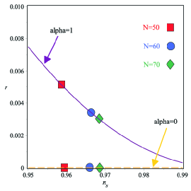
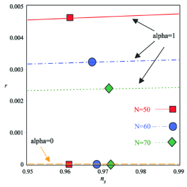
Figure 1: Tensor to scalar ratio versus the scalar spectral index for NMD model with the E-model (left panel) and T-model (right panel) potential.

4 Reheating

After inflation ends, the process of reheating take places. By consider this process we can investigate some constraints on the model’s parameter space. In this section, we obtain expressions for e-fold number and temperature of reheating era.

The e-fold number between the time of horizon crossing and end of inflation is written as

$$N_{hc}=\ln\bigg{(}\frac{a_{e}}{a_{hc}}\bigg{)},$$ (48)

where $a_{hc}$ and $a_{e}$ are scale factor at the horizon crossing and end of inflation, respectively.

We assume that at the end of reheating epoch, energy density of the universe is given by

$$\rho_{re}=\frac{\pi^{2}g_{re}}{30}T_{re}^{4},$$ (49)

where $g_{re}$ is effective number of relativistic particles at the end of reheating.

In this respect, the length of reheating is written as

$$N_{re}=\ln\bigg{(}\frac{a_{re}}{a_{e}}\bigg{)}=-\frac{1}{3(1+\omega_{eff})}\ln\bigg{(}\frac{\rho_{re}}{\rho_{e}}\bigg{)},$$ (50)

so that we substituted the relation $\rho\sim a^{-3(1+\omega_{eff})}$ at above equation. Where $\rho$ and $\omega_{eff}$ are energy density and effective equation of state, respectively.

Horizon crossing occurs at $a_{hc}H_{hc}=k$, where $k$ denotes wave number and $H_{hc}$ is Hubble parameter at horizon crossing during inflation. Then we can write

$$0=\ln\bigg{(}\frac{k}{a_{hc}H_{hc}}\bigg{)}=\ln\bigg{(}\frac{a_{e}}{a_{hc}}\frac{a_{re}}{a_{e}}\frac{a_{0}}{a_{re}}\frac{k}{a_{0}H_{hc}}\bigg{)},$$ (51)

where $a_{0}$ is scale factor of present epoch. Now, from Eqs. (48) and (50) we obtain

$$N_{hc}+N_{re}+\ln\bigg{(}\frac{a_{0}}{a_{re}}\bigg{)}+\ln\bigg{(}\frac{k}{a_{0}H_{hc}}\bigg{)}=0.$$ (52)

From conservation of entropy we can write

$$\frac{a_{0}}{a_{re}}=\bigg{(}\frac{43}{11g_{re}}\bigg{)}^{-\frac{1}{3}}\frac{T_{re}}{T_{0}},$$ (53)

where $T_{0}$ is the current temperature. From Eqs. (49) and (53) we obtain

$$\frac{a_{0}}{a_{re}}=\bigg{(}\frac{43}{11g_{re}}\bigg{)}^{-\frac{1}{3}}\bigg{(}\frac{\pi^{2}g_{re}}{30\rho_{re}}\bigg{)}^{-\frac{1}{4}}\frac{1}{T_{0}}.$$ (54)

In our framework, the energy density during the inflation epoch can be rewritten as follows

$$\rho=\frac{9H^{2}}{2\widetilde{M}^{2}}\dot{\phi}^{2}-\frac{3}{2}M_{p}^{2}H\phi(2\dot{\phi}+H\phi)+V(\phi).$$ (55)

Now by setting $\epsilon=1$, the energy density at the end of inflation phase is the following form

$$\rho_{e}=\bigg{(}\frac{2}{2+\phi_{e}^{2}}\bigg{)}V_{e},$$ (56)

where $\phi_{e}$ and $V_{e}$ are scalar field and potential at the end of inflation, respectively. Then from Eqs. (50) and (56) we have

$$\rho_{re}=\bigg{(}\frac{2}{2+\phi_{e}^{2}}\bigg{)}V_{e}\exp[-3(1+\omega_{eff})N_{re}].$$ (57)

$H_{hc}$ can be find from Eq. (26). Now by substituting $H_{hc}$ and Eqs. (54) and (57) in the Eq. (52) we can write the following expression for e-fold number of reheating era

$$N_{re} = \frac{4}{(1-3\omega_{eff})}\bigg{[}-N_{hc}-\ln\bigg{(}\frac{k_{hc}}{a_{0}}\bigg{)}+\frac{1}{2}\ln(8\pi^{2}P_{s}\vartheta_{s}c_{s}^{3})+\frac{1}{3}\ln\bigg{(}\frac{43}{11g_{re}}\bigg{)}$$ (58)

$$+\frac{1}{4}\ln\bigg{(}\frac{\pi^{2}g_{re}}{30}\bigg{)}+\ln T_{0}-\frac{1}{4}\ln\bigg{(}\frac{2V_{e}}{2+\phi_{e}^{2}}\bigg{)}\bigg{]}.$$

and from equations (49) and (57) we obtain the temperature during reheating

$$T_{re}=\bigg{(}\frac{60V_{e}}{\pi^{2}g_{re}(2+\phi_{e}^{2})}\bigg{)}^{\frac{1}{4}}\exp\bigg{[}-\frac{3}{4}(1+\omega_{eff})N_{re}\bigg{]}.$$ (59)

The scalar spectral index and wave number are related through $\phi$ with Eqs. (30), (48) and $a_{hc}H_{hc}=k$, therefore one can investigate $N_{re}$ and $T_{re}$ in terms of the scalar spectral index for each model.

4.1 E-model

First, we consider E-model potential defined in Eq. (40). As we know, in the small $\alpha$ and large $N$ limit, one can rewrite the potential as

$$V=V_{0}\bigg{[}1-2n\exp(-\sqrt{\frac{2}{3M_{pl}^{2}\alpha}}\phi)\bigg{]},$$ (60)

where we assume that $n=1$. We also need to the e-fold number that happen after a mode with wave number $k$. By substituting the above equation in the Eq. (14) we can obtain e-folding as function of $\phi$ which defined as following expression

$$N_{hc} \approx \frac{V_{0}}{M_{pl}^{4}\widetilde{M}^{2}}\bigg{[}-\frac{1}{4}\phi^{2}(\phi^{2}-4)+\frac{1}{2}(\phi^{4}+4\sqrt{6M_{pl}^{2}\alpha}\phi$$ (61)

$$+12M_{pl}^{2}\alpha-4)\exp\bigg{(}-\sqrt{\frac{2}{3M_{pl}^{2}\alpha}}\phi\bigg{)}\bigg{]}_{\phi_{hc}}^{\phi_{e}}.$$

Now, by plotting the e-fold number and temperature of reheating era versus the scalar spectral index we can study the parameters numerically. We consider the case with $\alpha=1$ for some values of effective equation of state. The results are shown in Figure (2).

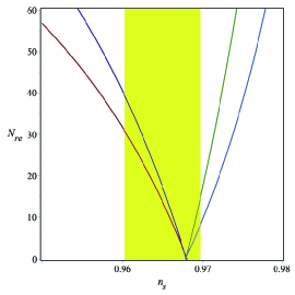
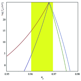
Figure 2: $N_{re}$ (left panel) and $T_{re}$ (right panel) as function of the scalar spectral index for E-model when $n=1$ with $\alpha=1$. In each panel, the red line corresponds to $\omega_{re}=-\frac{1}{3}$, the purple line to $\omega_{re}=0$, the green line to $\omega_{re}=\frac{2}{3}$ and the blue line to $\omega_{re}=1$. The yellow shaded region indicate the Planck 2018 constraint.

According to the picture, we can obtain constraints on the model s parameter space by adopting our results with the Planck 2018. The constrains on the E-model parameters are shown in Table 1.

Table 1: The ranges of e-fold number and temperature during reheating epoch for E-model potential which are consistent with the Planck 2018.

$n=1,\alpha=1$	$\omega_{eff}=-\frac{1}{3}$	$\omega_{eff}=0$	$\omega_{eff}=\frac{2}{3}$	$\omega_{eff}=1$
$N_{re}$	$<31$	$<39$	$<15$	$<8$
$\log(T_{re})$	$>15$	$>4$	$>22$	$>23$

4.2 T-model

Now, we consider T-model potential defined in Eq. (41). By substituting the potential in the Eq. (14) we can obtain e-folding as function of $\phi$ which defined as following expression

$$N_{hc} \approx V_{0}\bigg{[}12M_{pl}^{2}\alpha\log(\cosh(\frac{\phi}{\sqrt{6M_{pl}^{2}\alpha}}))+\frac{1}{4}(\phi^{4}-4)\cosh(\frac{\phi}{\sqrt{6M_{pl}^{2}\alpha}})^{-2}$$ (62)

$$-8\sqrt{6M_{pl}^{2}\alpha}\phi\tanh(\frac{\phi}{\sqrt{6M_{pl}^{2}\alpha}})-\phi^{4}+4\phi^{2}\bigg{]}_{\phi_{hc}}^{\phi_{e}}.$$

We consider $\alpha=1$ and plot the e-fold number and temperature of reheating era versus the scalar spectral index. The results are shown in Figure (3). Therefore, we obtain some constraints on the model s parameter space. The constrains on the T-model parameters are shown in Table 2.

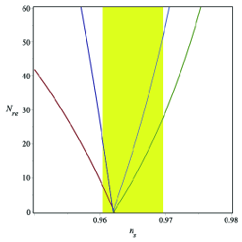
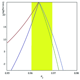
Figure 3: $N_{re}$ (left panel) and $T_{re}$ (right panel) as function of scalar spectral index for T-model when $n=1$ with$\alpha=1$. In each panel, the red line corresponds to $\omega_{re}=-\frac{1}{3}$, the purple line to $\omega_{re}=0$, the green line to $\omega_{re}=\frac{2}{3}$ and the blue line to $\omega_{re}=1$. The yellow shaded region indicate the Planck 2018 constraint.

Table 2: The ranges of e-fold number and temperature during reheating epoch for T-model potential which are consistent with the Planck 2018.

$n=1,\alpha=1$	$\omega_{eff}=-\frac{1}{3}$	$\omega_{eff}=0$	$\omega_{eff}=\frac{2}{3}$	$\omega_{eff}=1$
$N_{re}$	$<8$	$<20$	$<52$	$<27$
$\log(T_{re})$	$>20$	$>16$	$>7.5$	$>12$

4.3 Post-Inflationary era

The reheating evolution of the Horndeski models is much different than the usual minimal coupling theory. The scalar field (inflaton) oscillates very fast and coherently around the minimum of its potential. The averaged expansion of the universe is given by (for more details refer to Refs. [34,43,44])

$$\bar{H}(t,\omega_{re})=\frac{1}{\frac{3}{2}(1+\bar{\omega}_{re})(t-t_{end})+H^{-1}_{end}},$$ (63)

for $t_{end}<t<t_{re}$. The averaged equation of state ($\bar{\omega}_{re}$) after inflationary era is determined by oscillating behavior of the scalar field about the minimum. The above expression for $\bar{H}$ imply a different relation for $\bar{\omega}_{re}$. As a result of Ref. [34], for the non-minimal derivative models, one can obtain different negative values for the equation of state. In Fig. (4) we plot time evolution of the Hubble parameter for the possible values of the equation of state.

On the other hand, during the slow-roll phase we have a dual description for the tensor-to-scalar ratio in the non-minimal derivative and usual minimal coupling scenario. However, this degeneracy breaks by different value of the reheating temperature and equation of state parameter when the reheating phase is taken into account.

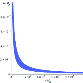
Figure 4: Time evolution of the Hubble parameter for the possible values of the equation of state.

5 Summary

In this letter, we have considered a class of non-minimal derivative inflationary model. We focused on both the E-model and T-model as generalized models of $\alpha$-attractors. We have obtained the scaler spectral index and tensor to scaler ratio in the models. As shown above, in the small $\alpha$ and large $N$ limit, the model with E-model potential predicts $n_{s}\approx 1-\frac{2}{N}$ and $r\approx\frac{12\alpha}{N^{2}}$ where there is an attractor behavior. However, the value of the $n_{s}$ and $r$ predicted by T-model, has some deviation from the corresponding terms in E-model. We analyzed the parameters numerically for $n=1$ and compared our results with observations. We have found that the models for large N are consistent with the Planck data.

Moreover, we have studied the reheating phase in the NMD model. We obtained e-fold number and temperature during reheating in terms of scalar spectral index for both E-model and T-model. We also analyzed the parameters numerically for $n=1$ with $\alpha=1$ and compared the results with observational data. As shown in Table (1,2), we have obtained some constraints on the model’s parameter space by adopting our results with Planck 2018.

References

- [1] A. A. Starobinsky, Phys. Lett. B 91 99 (1980).
- [2] A. H. Guth, Phys. Rev. D 23, 347 (1981).
- [3] A. D. Linde, Phys. Lett. B 108, 389 (1982).
- [4] A. Albrecht and P. J. Steinhardt, Phys. Rev. Lett. 48, 1220 (1982).
- [5] A. D. Linde, Phys. Lett. B 129, 177 (1983).
- [6] A. D. Linde, Harwood Academic, Chur, Switzerland, (1990) [hep-th/0503203].
- [7] J. E. Lidsey, A. R. Liddle, E.W. Kolb, E. J. Copeland, T. Barreiro, and M. Abney , Rev. Mod. Phys. 69, (1997) 373.
- [8] A. Liddle and D. Lyth, Cambridge, England, (2000).
- [9] D. H. Lyth and A. R. Liddle, Cambridge University Press, Cambridge, England, (2009).
- [10] P. A. R. Ade et al. [BICEP2 and Planck Collaborations], [arXiv:1502.00612 [astro-ph.CO]].
- [11] Y. Akrami et al. arXiv preprint arXiv:1807.06211 (2018).
- [12] P. A. R. Ade et al. [Planck Collaboration], arXiv:1502.02114 [astro-ph.CO].
- [13] WMAP collaboration, G. Hinshaw et al., Astrophys. J. Suppl. 208 (2013) 19 [arXiv:1212.5226] [INSPIRE].
- [14] R. Kallosh and A. Linde, JCAP 07 (2013) 002 [arXiv:1306.5220] [INSPIRE].
- [15] R. Kallosh and A. Linde, JCAP 12 (2013) 006 [arXiv:1309.2015] [INSPIRE].
- [16] S. Ferrara, R. Kallosh, A. Linde and M. Porrati, Phys. Rev. D 88 (2013) 085038 [arXiv:1307.7696] [INSPIRE].
- [17] R. Kallosh, A. Linde and D. Roest, JHEP 11 (2013) 198 [arXiv:1311.0472] [INSPIRE].
- [18] R. Kallosh, A. Linde and D. Roest, JHEP 08 (2014) 052 [arXiv:1405.3646] [INSPIRE].
- [19] S. Cecotti and R. Kallosh, JHEP 05 (2014) 114 [arXiv:1403.2932] [INSPIRE].
- [20] R. Kallosh, A. Linde and D. Roest, Phys. Rev. Lett. 112 (2014) 011303 [arXiv:1310.3950] [INSPIRE].
- [21] M. Galante, R. Kallosh, A. Linde and D. Roest, Phys. Rev. Lett. 114 (2015) 141302 [arXiv:1412.3797] [INSPIRE].
- [22] R. Kallosh and A. Linde, [arXiv:1503.06785].
- [23] R. Kallosh, A. Linde and D. Roest, J. High Energy Phys. 09 (2014) 062. 36.
- [24] J. Joseph, M. Carrasco, R. Kallosh and A. Linde, Phys. Rev. D 92 (2015) 063519. 38.
- [25] R. Kallosh, A. Linde, D. Roest and T. Wrase, J. Cosmol. Astropart. Phys. 1611 (2016) 046.
- [26] J. Martin and C. Ringeval, Phys. Rev. D 82, 023511 (2010) [arXiv:1004.5525 [astro-ph.CO]].
- [27] P. Adshead, R. Easther, J. Pritchard and A. Loeb, JCAP 1102, 021 (2011) [arXiv:1007.3748 [astro-ph.CO]].
- [28] J. Mielczarek, Phys. Rev. D 83, 023502 (2011) [arXiv:1009.2359 [astro-ph.CO]].
- [29] S. Dodelson and L. Hui, Phys. Rev. Lett. 91, 131301 (2003) [astro-ph/0305113].
- [30] R. Easther and H. V. Peiris, Phys. Rev. D 85, 103533 (2012) [arXiv:1112.0326 [astro-ph.CO]].
- [31] J. Martin, C. Ringeval, and V. Vennin, Phys.Rev.Lett. 114, 081303 (2015), arXiv:1410.7958 [astro-ph.CO].
- [32] D. I. Podolsky, G. N. Felder, L. Kofman and M. Peloso, Phys. Rev. D 73, 023501 (2006) [hep-ph/0507096].
- [33] T. Harko, F. S. N. Lobo, E. N. Saridakis and M. Tsoukalas, Physical Review D 95, no. 4 (2017): 044019.
- [34] I.Dalianis, G.Koutsoumbas, K.Ntrekis, and E.Papantonopoulos, Journal of Cosmology and Astroparticle Physics 2017, no. 02 (2017): 027.
- [35] R. L. Arnowitt, S. Deser, andC.W. Misner, Physical Review A: Atomic,Molecular and Optical Physics, vol. 117, no. 6, p. 1595, 1960.
- [36] V. F. Mukhanov, H. A. Feldman, and R. H. Brandenberger, Theory of cosmological perturbations, Physics Reports, vol. 215, no. 5-6, pp. 203 333, 1992.
- [37] C. Cheung, A. L. Fitzpatrick, J. Kaplan, L. Senatore, and P. Creminelli, Journal of High Energy Physics, vol. 2008, no. 03, article no. 014, 2008.
- [38] Shojaee, R., Nozari, K., and Darabi, F. (2018). More on the Non-Gaussianity of Perturbations in a Nonminimal Inflationary Model. Advances in High Energy Physics, 2018 [arXiv:1808.04259].
- [39] A. De Felice and S. Tsujikawa, Journal of Cosmology and Astroparticle Physics, vol. 2011, no. 4, article 029, 2011.
- [40] S. Tsujikawa, Physical Review D: Particles, Fields, Gravitation and Cosmology, vol. 85, Article ID 083518, 2012.
- [41] D. Seery and J. E. Lidsey, Journal of Cosmology and Astroparticle Physics, vol. 2005, no. 6, article no. 003, 2005.
- [42] K. Nozari and N. Rashidi, The Astrophysical Journal 863, no. 2 (2018): 133.
- [43] R. Jinno, K. Mukaida and K. Nakayama, JCAP 1401 (2014) 031, [arXiv:1309.6756 [astro-ph.CO]].
- [44] Y. Ema, R. Jinno, K. Mukaida and K. Nakayama, JCAP 1510, no. 10, 020 (2015), [arXiv:1504.07119 [gr-qc]].