Robust Dynamical Decoupling for the Manipulation of a Spin Network via a Single Spin

Abstract

High-fidelity control of quantum systems is crucial for quantum information processing, but is often limited by perturbations from the environment and imperfections in the applied control fields. Here, we investigate the combination of dynamical decoupling (DD) and robust optimal control (ROC) to address this problem. In this combination, ROC is employed to find robust shaped pulses, wherein the directional derivatives of the controlled dynamics with respect to control errors are reduced to a desired order. Then, we incorporate ROC pulses into DD sequences, achieving a remarkable improvement of robustness against multiple error channels. We demonstrate this method in the example of manipulating nuclear spin bath via an electron spin in the NV center system. Simulation results indicate that ROC based DD sequences outperform the state-of-the-art robust DD sequences. Our work has implications for robust quantum control on near-term noisy quantum devices.

Introduction.–Dynamical decoupling (DD) is a well-established open-loop quantum control technique [1] that has substantial applications, such as protecting quantum coherence [2, 3, 4, 5, 6], implementing high-fidelity quantum gates [7, 8, 9, 10], probing noise spectrum [11, 12] and quantum sensing [13, 14, 15]. In its basic form, a DD sequence comprises a series of instantaneous pulses on the system of concern, separated by certain interpulse delays. However, actual pulses must have bounded strengths and hence can not be really instantaneous. Besides, there are inevitable pulse control imperfections, including off-resonant errors and control field fluctuations. These non-ideal factors can cause a DD scheme fail to achieve the expected performance [16]. To overcome this problem, a commonly used approach is to apply pulses along different spatial directions to let the error of one pulse be compensated by other pulses [17, 18, 19]. Also, one can combine DD with composite pulses (CP) which are robust against operational errors [20]. These efforts have yielded in the past decades a significant number of robust DD sequences, such as the XY8 [17], CDD [21], KDD [22], UR [23], and random-phase [24] sequences. However, since fighting against noise effects on current noisy intermediate-scale quantum [25] devices remains a compelling challenge, robust DD continues to be a significant research problem of strong interest.

Generally, for establishing a well-behaved robust DD sequence, several issues are particularly worth considering [1, 16]. First, a satisfactory control fitness profile against imperfections resembles that shown in Fig. 1(a), i.e., the central robust region should be as broad and flat as possible. Second, it is desirable that the DD sequence can resist several types of imperfections simultaneously. This is a natural requirement because in realistic situations various perturbations exist concurrently. Third, the widths of the basic pulses need to be much shorter than the interpulse delays. However, present DD sequences usually do not meet all of these requirements. Take CP based DD as an example, representative CPs like CORPSE [26] or BB1 [27] correct only a single error type, and concatenated CPs can correct simultaneously existing errors but only at the price of larger pulse-widths [28], hence the CP technique does not easily lend itself to incorporating the desired robustness features.

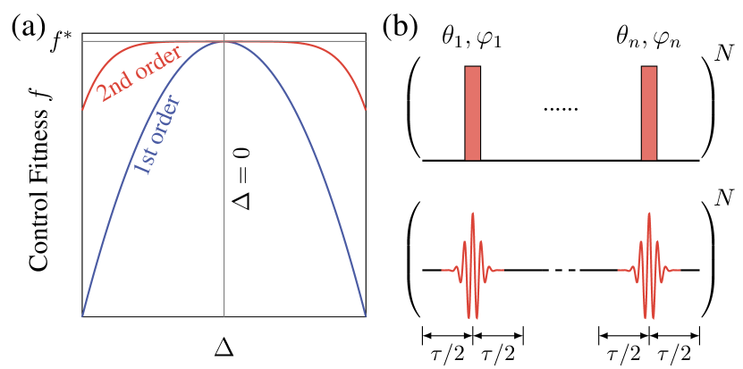
Figure 1: (a) Robustness against pulse imperfection. The higher level to which the derivatives of the fitness function with respect to the imperfections are reduced, the better. (b) Typical DD sequence structure combining a series of basic pulses with arbitrary shapes.

In this work, we show that combining DD with robust optimal control (ROC) provides a general and effective way to enhance robustness for multiple pulse errors. Here, ROC is in essence quantum optimal control [29] with the additional robustness constraint requiring that the leading order effects of the imperfections are minimized. Our basic idea is to replace the hard pulses in DD with robust shaped pulses that are optimized via ROC algorithms [30]. The whole DD sequence is able to exhibit much improved error tolerance. As demonstration, we apply this framework to the problem of manipulating a spin network via a single spin. In defect-based systems, such as nitrogen-vacancy (NV) center in diamond [13, 31, 32] and silicon-based quantum dots [33, 34], a frequently encountered control scenario is to use a single probe spin to explore properties of a quantum spin network in the proximity. This central spin can function as a polarizer, detector, or actuator [35, 36], often resorting to the DD technique. Here, in particular, we focus on the task of nuclear spin detection and hyperpolarization by driving the electron spin only. Our numerical simulations show that ROC based DD sequences outperform the best robust DD sequences available so far.

Robust DD.–Consider a single spin as the system $S$ coupled to a spin network as its interacting environment $E$. In the resonantly rotating frame of $S$, the free evolution Hamiltonian is $H=H_{SE}+H_{E}$. In DD, control is acted on $S$ alone, which is implemented by a transversely applied time-dependent field $u(t)=(u_{x}(t),u_{y}(t))$. Let $S_{\alpha}=\sigma_{\alpha}/2$ ($\alpha=x,y,z$), $\sigma_{\alpha}$ being the Pauli operators, then the control Hamiltonian is $H_{C}(u(t))=u_{x}(t)S_{x}+u_{y}(t)S_{y}$. We shall assume the hierarchy in the coupling strengths, $H_{C}\gg H_{SE}\gg H_{E}$. As such, we can just omit the weak term $H_{E}$ as it does not appear in the DD problem to the lowest order [37]. The general goal of DD is to find a suitable control sequence to synthesize a target effective dynamics of interest. However, in the actual implementation, DD must take into account control imperfections, as realistic pulse profiles inevitably incorporate pulse-shaping errors due to finite-power and finite-bandwidth constraints in hardware. Here, we view these imperfections as perturbations and write the perturbed Hamiltonian as

$$H(t)=H_{SE}+H_{C}(u(t))+\sum_{i}\epsilon_{i}V_{i}(t),$$ (1)

in which $\left\{V_{i}(t)\right\}$ are noise operators, and $\left\{\epsilon_{i}\right\}$ are their corresponding weights. Specifically, we shall consider in this work mainly off-resonant and control amplitude errors, i.e., $V_{1}=\Delta_{\max}S_{z}$ and $V_{2}(t)=H_{C}(u(t))$, where $\Delta_{\max}$ represents the maximum detuning. Our goal is to devise a robust DD protocol that realizes a given control target with sufficiently high accuracy for a broad range of noise strengths.

We start from a typical DD sequence of the structure shown in Fig. 1(b). The sequence is built based on a set of basic pulses $\left\{u_{\theta,0}(t):0\leq\theta\leq\pi\right\}$, here $u_{\theta,0}(t)$ represents a control pulse intended to effect a single-qubit rotation $R_{0}(\theta)$ with angle $\theta$ and phase $\phi=0$. More specifically, the sequence consists of sequentially combining $n$ pulses from the basic pulse set, each with a phase shift, into a DD block, and then repeating this block for $N$ times. The $k$th pulse in the DD block is denoted as $u_{k}=u_{\theta_{k},\phi_{k}}$, obtained from $u_{\theta_{k},0}$ by a phase shift $\phi_{k}$. Adjacent pulses are time separated by $\tau$, and we shall assume that for each pulse $u_{\theta_{k},\phi_{k}}$, its pulse-width $\tau_{u_{k}}$ is small compared with $\tau$.

We want to quantify the control robustness of the considered DD sequence. First let us look into the errors arisen in applying a single pulse $u_{\theta,\phi}$. The real controlled time evolution operator in the presence of perturbations is approximately $e^{-iH_{SE}\tau_{u}/2}U_{\theta,\phi}e^{-iH_{SE}\tau_{u}/2}$ with $U_{\theta,\phi}=\mathcal{T}e^{-i\int_{0}^{\tau_{u}}dt(H_{C}(t)+\epsilon_{1}V_{1}+\epsilon_{2}V_{2}(t))}$, where we only allow for the first-order effect of $H_{SE}$ during the short period of pulse control [38]. According to the Dyson perturbative theory [39], $U_{\theta,\phi}$ can be expanded as the series $U_{\theta,\phi}=R_{\phi}(\theta)+\sum_{i_{1}}\epsilon_{i_{1}}\mathcal{D}_{U_{\theta,\phi}}^{(1)}(V_{i_{1}})+\sum_{i_{1},i_{2}}\epsilon_{i_{1}}\epsilon_{i_{2}}\mathcal{D}_{U_{\theta,\phi}}^{(2)}(V_{i_{1}},V_{i_{2}})+\cdots$, where the $m$th ($m\geq 1$) order terms $\mathcal{D}_{U_{\theta,\phi}}^{(m)}(V_{i_{1}},...,V_{i_{m}})=(-i)^{m}R_{\phi}(\theta)\int_{0}^{\tau_{u}}dt_{1}\cdots\int_{0}^{t_{m-1}}dt_{m}\widetilde{V}_{i_{1}}(t_{1})\cdots\widetilde{V}_{i_{m}}(t_{m})$ for $i_{1},...,i_{m}=1,2$ are referred to as the $m$th order directional derivatives [30], characterizing the perturbative effects due to the noise generators $\left\{V_{i}\right\}$. Here, $\widetilde{V}_{i}(t)=U^{\dagger}_{C}(t)V_{i}(t)U_{C}(t)$ with $U_{C}(t)=\mathcal{T}e^{-i\int_{0}^{t}dsH_{C}(s)}$. For any $m$ and for any time-ordered operators $V_{i_{1}},...,V_{i_{m}}$, we can derive that [38]

$$\mathcal{D}_{U_{\theta,\phi}}^{(m)}=e^{-i\phi S_{z}}\mathcal{D}_{U_{\theta,0}}^{(m)}e^{i\phi S_{z}}.$$ (2)

Thus there is $\left\|\mathcal{D}_{U_{\theta,\phi}}^{(m)}\right\|^{2}=\left\|\mathcal{D}_{U_{\theta,0}}^{(m)}\right\|^{2}$, implying that we need only to consider the robustness of the basic pulses.

Now, for the whole DD block, the real propagator goes

$$U_{\text{DD}}=W_{n}U_{\theta_{n},\phi_{n}}W_{n}\cdots W_{1}U_{\theta_{1},\phi_{1}}W_{1},$$ (3)

where $W_{k}=e^{-i(H_{SE}\tau/2+\epsilon_{1}V_{1}(\tau-\tau_{u_{k}})/2)}$ is the free evolution operator which has incorporated the $H_{SE}$ evolution [38]. It is then clear that the errors in $U_{DD}$ in Eq. (6) include detuning errors in $W_{k}$ as well as both detuning and control amplitude errors in $U_{\theta_{k},\phi_{k}}$, up to first-order approximation with respect to $H_{SE}$. Hence, there are two feasible approaches toward robust DD. On the one hand, DD seeks to use a properly designed phase modulation strategy so that the errors will cancel rather than accumulate. Notable examples include the two-axis XY-family [17], the multi-axis UR [23], and the random-phase [24] or correlated-random-phase [40] sequences. On the other hand, by minimizing the magnitudes of the directional derivatives $\mathcal{D}_{U_{\theta_{k},0}}^{(m)}$, the robustness of the pulses $u_{\theta_{k},\phi_{k}}(t)$ are enhanced, and the total error of the full sequence will be accordingly decreased. Furthermore, if both approaches are taken simultaneously, we anticipate that the DD robustness property will get improved to an even larger degree.

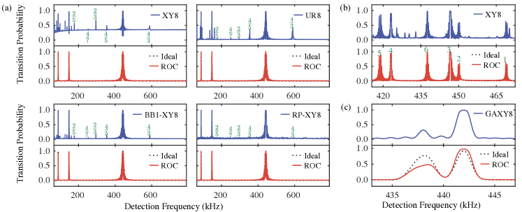
Figure 2: Simulated spectra of detecting nuclear spins, where the control imperfection parameters are set as detuning $8\%\times\Omega_{\max}$, amplitude error $8\%\times\Omega_{\max}$, and $\pi$ pulse with a limit width $1/(2\Omega_{\max})=20~{}$ns. The number of cycles for (a), (b), and (c) are 96, 32, and 64, respectively. (a) Signal from a single spin with $\omega_{I}=2\pi\times 441.91~{}$kHz detected by various DD sequences. The results for XY8, UR8, BB1-XY8, RP-XY8 and their ROC counterparts are presented. Clearly, using our ROC pulses excellently solves the baseline distortion problem and eliminates the spurious peaks (green marker) that are located at $2\omega_{I}/k$ and $4\omega_{I}/k$ ($k$ is odd) [41]. (b) Signal from six spins (see simulation parameters in [38]). The miscellaneous peaks appeared in applying XY8 greatly hamper the identification of each spin, but can be circumvented by ROC-XY8. (c) Signal from two spectrally close spins with $\omega_{I}^{1}=2\pi\times 441.91~{}$kHz and $\omega_{I}^{2}=2\pi\times 437.53~{}$kHz. It can be seen that, the ROC based sequence shows better robustness against imperfections in resolving the two spins.

A particularly effective approach for devising shaped pulses that are robust to several simultaneously existing perturbations is the ROC algorithm developed in Ref. [30]. In our subsequent numerical simulations, we shall generally follow this approach. Basically, we attempt to solve the following multi-objective optimization problem: for a given target rotation angle $\theta$, to optimize the shape of the pulse $u=u_{\theta,0}(t)$ to (i) maximize the fidelity between the unperturbed propagator and the target rotation $R_{0}^{\dagger}(\theta)$, and meanwhile (ii) minimize $\left\|\mathcal{D}_{U_{\theta_{k},0}}^{(m)}\right\|^{2}$ for $m$ up to a certain order. One can employ either the known gradient ascent pulse engineering algorithm [42] or gradient-free methods like the differential evolution [43, 44, 45] algorithm to perform the pulse search. Note that in the entire space of admissible control functions, there may exist plenty of solutions that can accomplish the same control goal. However, as a realistic pulse generator has limited bandwidth, we shall exclude consideration of abruptly changing pulse shapes. We put the algorithm implementation details in Supplementary Materials [38]. In the next section, we study the applications of our optimized robust pulses.

Applications.–Consider the system of an electron spin $S$ ($S=1/2$) of an NV center in diamond and surrounding nuclear spins $I$ ($I=1/2$). The system is under a static magnetic field applied along the NV axis which is, by convention, defined as the $\hat{z}$ axis. The electron spin is subject to intermediately applied microwave control field $u(t)$. In a rotating frame with respect to $\Omega_{S}S_{z}$, the Hamiltonian after the secular approximation reads

$$H=\sum_{j}\Omega_{I}I^{j}_{z}+\sum_{j}S_{z}(A^{j}_{zz}I_{z}^{j}+A^{j}_{zx}I_{x}^{j})+H_{C}(u(t)),$$ (4)

in which $\Omega_{S}$ ($\Omega_{I}$) denotes the electron (nuclear) Larmor frequency, $A_{zz}$ and $A_{zx}$ are the hyperfine coupling strengths. In our numerical studies, we assume the existence of a minimum switching time $t_{\min}=1$ ns for pulse modulation and require all control amplitudes to be bounded by $\Omega_{\max}=2\pi\times 25$ MHz. Three common pulse imperfections, namely detuning, control amplitude error, and finite pulse-width, are under consideration. The details of pulse optimization can be found in Supplementary Materials [38].

First, we investigate the detection of nuclear spins via the central electron spin. Nuclear spins exist naturally in abundance in NV center systems, providing possible additional quantum resources [46, 47, 15]. A prerequisite to exploit this potential is to detect and characterize them, usually with the aid of the electron spin. Ideally, the $j$th nuclear spin with the effective Larmor frequency $\omega_{I}^{j}=\Omega_{I}+A_{zz}^{j}/2$ can induce a sharp electron signal in the observed spectrum, by applying a multi-pulse DD sequence on the electron spin with the interpulse delay $\tau=k\pi/\omega_{I}^{j}$ ($k$ is odd) [13]. Nevertheless, addressing and controlling nuclear spins is challenging as the spins are generally embedded in noisy spin bath, and the inevitable pulse imperfections can induce spurious peaks [41] and distortion of the spectrum [48]. To avoid false identification, many robust DD sequences were proposed [23, 24, 22, 48, 49]. However, when the pulse imperfections are relatively large and exist simultaneously, we find that the performance of the present robust DD sequences can be further improved by using ROC pulses.

As an initial demonstration, let us consider the situation of detecting a single ¹³C nuclear spin. The simulated spectra with using four representative robust DD sequences are shown in Fig. 2(a). For conventional XY8 sequence, there exist miscellaneous errors in the signal including, the tilted baseline that causes severely reduced contrast, the phase-distorted resonant peaks, and the spurious peaks appearing due to finite pulse-width and detuning effects [41], so the spectrum is hard to analyze and identify. Substituting the square-shaped $\pi$ pulses with BB1 in XY8 (BB1-XY8) [27], or using the UR8 sequence [23], improves the signal, but still does not solve the spurious peak problem. A recently proposed random-phase XY8 (RP-XY8) sequence [24] can largely suppress the spurious peaks and maintain the signal contrast, but still induce dense small miscellaneous peaks near the baseline. It is found that, for all these sequences, if implemented with our ROC pulses ($t_{\text{ROP}}=80~{}$ns), then the errors almost disappear, giving a rather clean spectrum close to the ideal one.

Next, we consider detecting multiple ¹³C nuclear spins. The case of six nuclear spins is presented in Fig. 2(b). As can be seen from the spectrum, a bunch of spurious peaks exist, making it a difficult task to identify the spins. This gets even worse when the cycle number $N$ is large. Again, combining XY8 with our ROC pulses suppresses all the unwanted peaks to a satisfactory extent. As an additional demonstration example, we have considered the problem of detecting two spectrally close nuclear spins. This situation demands good selectivity of the control sequence in addressing the nuclear spins individually. Recently, Ref. [50] proposed an effective soft temporal modulation sequence named Gaussian AXY8, which has better selectivity than conventional XY8. However, when taking into account of pulse imperfections, distortions occur in the transition probabilities of the spins, leading to off-resonant side peaks and hence reducing the signal contrast, as shown in Fig. 2(c). We thus test with our ROC pulses, finding that the side peaks around the spin resonances are all removed, and consequently the two spins are well resolved; see details in Supplementary Materials [38]. Clearly, our approach is of great benefit when fitting dense signals for many close nuclear spins, especially when spurious resonances exist.

Now, we turn to the application to dynamical nuclear polarization (DNP) of the nuclear spins. DNP aims to transfer the almost perfect polarization of the optically initialized electron spin to its surrounding nuclear spins; see Fig. 3(a). This could result in an enhancement of the nuclear signal by several orders of magnitude, which is crucial for a variety of quantum technologies such as magnetic resonance imaging [51]. The goal of achieving high-efficiency DNP in NV centers in diamond has attracted a lot of interests in recent years but remains technically challenging. Key factors affecting effective polarization include: the large spectral random orientation of the NV center axes and Rabi power imperfection. For example, conventionally DNP uses the Hartmann-Hahn resonance [52], the corresponding NOVEL sequence [53] works only in a narrow frequency range. Hence, there have been efforts made in devising more robust DNP protocols [54, 55, 52]. A significant advance was made by Ref. [56], which put forward a Hamiltonian engineering based approach termed PulsePol, featuring both fast polarization and excellent robustness. Yet, we find that the results presented in Ref. [56] can still be improved, with using our ROC shaped pulses.

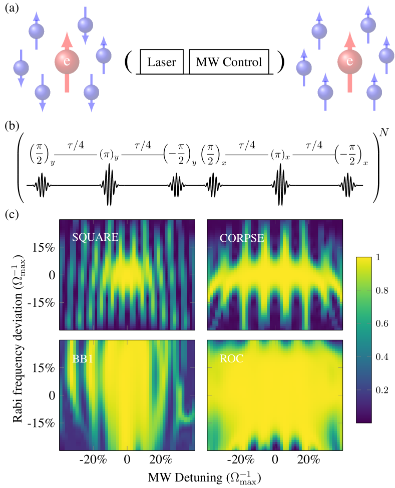
Figure 3: (a) Schematics of the microwave (MW) pulse sequence on the electron spin for pulsed polarization transfer to the surrounding nuclear spins. (b) The PulsePol sequence. As stated, the pulse duration should not take a large fraction of the free evolution time. (c) Comparison of error-resistance of four different PulsePol sequences.

For simplicity, we consider a single electron coupled to a single nuclear spin. The PulsePol sequence, as shown in Fig. 3(b), consists of $N$ cycles each with four $\pi/2$-pulses and two $\pi$-pulses, and operates for a choice of pulse spacing $\tau=l\pi/\omega_{I}$ for odd $l$. Ideally, it produces an effective flip-flop Hamiltonian as $H_{\text{eff}}=\alpha A_{zx}(S_{+}I_{-}+S_{-}I_{+})$, where $S_{\pm}=S_{x}\pm iS_{y}$, $I_{\pm}=I_{x}\pm iI_{y}$. As such, full polarization transfer is achieved at time $2N\tau=1/(\alpha A_{zx})$. However, because real pulses take a finite time, the free evolutions between the pulses need be adjusted according to $\tau_{\text{free}}=\tau-4t_{\pi/2}-2t_{\pi}$, where $t_{\pi/2}$ and $t_{\pi}$ denote the time length of the $\pi/2$ and $\pi$-pulses. As a consequence, the number of cycles $N$ required for full polarization transfer varies depending on the specific pulses used. In our simulations, we compare the robustness performance achieved from using four different realizations of the rotations, namely squared, CORPSE, BB1, and our ROC pulses. The simulations are implemented with the coupling strength $A_{zx}=0.03$ MHz, the resonance $l=5$, and the same cycle number $N=29$. The results are shown in Fig. 3(c). First, we clearly see that the robustness of PulsePol for using rectangular pulses is the worst. Then, the performance can be improved against detuning errors for CORPSE or against Rabi frequency errors for BB1. Finally, best results are achieved with our ROC pulses. There is a rather large flat central area of the robustness profile: the flat region satisfying $f\geq 0.99$ covers the entire error range of $\pm 5$ MHz detuning and $\pm 10\%$ Rabi frequency deviation.

Conclusion.–We have presented a flexible and effective framework for integrating DD with ROC. Unlike hard pulses, shaped pulses produced by ROC with smooth constraints are friendly to hardware implementation. In principle, ROC pulses can be incorporated into any DD sequence for robustness improvement. This is confirmed in our test examples of nuclear spin bath detection and hyperpolarization on NV center systems. Our method is ready to be exploited in many other spin network related problems, such as creating collective quantum memory [57], probing thermalization [58], exploring condensed matter phenomena [59] and studying magnetic dynamics of nanoparticles [60]. ROC based DD sequences can resist multiple errors simultaneously. This is especially important for near-term noisy quantum devices. For instance, recent benchmark experiments in superconducting qubits have identified real coexisting error channels as well as their respective contribution [61, 62], which are to be compensated for realization of high-fidelity quantum computing. Therefore, a meaningful extension of the current work is to explore how to achieve best robustness given knowledge of error channels and their weights. Lastly and rather importantly, future research could explore novel ROC strategies that can deal with time-dependent perturbations, which is a key ingredient to allowing robust DD to find a broader range of application scenarios [63, 64].

Acknowledgments. This work was supported by the National Natural Science Foundation of China (Grants No. 11975117, No. 92065111 and No. 12004037), and Guangdong Provincial Key Laboratory (Grant No. 2019B121203002).

Supplementary Material

I Analysis of the Effects of Control Imperfections on DD

In the resonantly rotating reference frame of $S$, the controlled system has the following Hamiltonian

$$H(t)=H_{E}+H_{SE}+H_{C}(u(t))+\epsilon_{1}V_{1}+\epsilon_{2}V_{2}(t).$$ (5)

Here, the meaning of each term is as described in the main text. For the sake of simplicity $H_{E}$ will not be written explicitly. The real propagator of the DD block in the presence of perturbations is written as

$$U_{\text{DD}}=W_{n}U_{\theta_{n},\phi_{n}}W_{n}\cdots W_{1}U_{\theta_{1},\phi_{1}}W_{1},$$ (6)

where $W_{k}=e^{-i(H_{SE}+\epsilon_{1}V_{1})(\tau-\tau_{u_{k}})/2}$ is the free evolution propagator, and $U_{\theta_{k},\phi_{k}}=\mathcal{T}e^{-i\int_{0}^{\tau_{u_{k}}}dtH(t)}$ is the real propagator for the $k$th pulse $u_{\theta_{k},\phi_{k}}(t)$. Because $H_{SE}$ is small in terms of the short pulse-width $\tau_{u_{k}}$, then to first order approximation, there is $U_{\theta_{k},\phi_{k}}=e^{-iH_{SE}\tau_{u_{k}}/2}\mathcal{T}\exp\left(-i\int_{0}^{\tau_{u_{k}}}dt\left[H_{C}(u(t))+\epsilon_{1}V_{1}+\epsilon_{2}V_{2}(t)\right]\right)e^{-iH_{SE}\tau_{u_{k}}/2}.$ The $H_{SE}$ evolutions can be incorporated into the free evolution operators $W_{k}$, so they evolve for the right amount of time. Accordingly, we only need to analyze

$$U_{\theta_{k},\phi_{k}}=\mathcal{T}\exp\left(-i\int_{0}^{\tau_{u_{k}}}dt\left[H_{C}(u_{\theta_{k},\phi_{k}}(t))+\epsilon_{1}V_{1}+\epsilon_{2}V_{2}(t)\right]\right),$$

which we do in the following.

First, for pulse $u_{\theta,\phi}(t)$, in the absence of perturbations, we denote the ideal time-evolution operator by

$$U^{\text{ideal}}_{\theta,\phi}(t)=\mathcal{T}\exp\left\{-i\int_{0}^{\tau_{u}}dtH_{C}(u_{\theta,\phi}(t))\right\},$$ (7)

Because $u_{\theta,\phi}$ is just $u_{\theta,0}$ phase shifted by $\phi$, so $H_{C}(u_{\theta,\phi}(t))=e^{-i\phi S_{z}}H_{C}(u_{\theta,0}(t))e^{i\phi S_{z}}$. There are: (i) for any time $t$, $U^{\text{ideal}}_{\theta,\phi}(t)=e^{-i\phi S_{z}}U^{\text{ideal}}_{\theta,0}(t)e^{i\phi S_{z}}$ and (ii) $U^{\text{ideal}}_{\theta,\phi}(\tau_{u})=R_{\phi}(\theta)$.

Now consider the presence of perturbations. To separate out the deviation of the real propagator $U_{\theta,\phi}(t)$ from the ideal propagator $U^{\text{ideal}}_{\theta,\phi}(t)$ caused by $V_{1}$ and $V_{2}(t)$, it is convenient to work in the toggling frame, i.e., $U_{\theta,\phi}(t)=U_{C}(t)U_{\text{tog}}(t)$, where $U_{C}(t)=\mathcal{T}e^{-i\int_{0}^{t}dsH_{C}(u_{\theta,\phi}(s))}$, and the toggling frame propagator $U_{\text{tog}}(t)=\mathcal{T}e^{-i\int_{0}^{t}ds(\epsilon_{1}\widetilde{V}_{1}(s)+\epsilon_{2}\widetilde{V}_{2}(s))}$ with $\widetilde{V}_{i}(s)=U^{\dagger}_{C}(s)V_{i}(s)U_{C}(s)$ can be expanded with the perturbative operators. This leads to the Dyson series

$$U^{\text{real}}_{\theta,\phi}(\tau_{u})=R_{\phi}(\theta)+\sum_{i_{1}}\epsilon_{i_{1}}\mathcal{D}_{U_{\theta,\phi}}^{(1)}(V_{i_{1}})+\sum_{i_{1},i_{2}}\epsilon_{i_{1}}\epsilon_{i_{2}}\mathcal{D}_{U_{\theta,\phi}}^{(2)}(V_{i_{1}},V_{i_{2}})+\cdots,$$ (8)

where the directional derivatives have the following expression

$$\mathcal{D}_{U_{\theta,\phi}}^{(m)}(V_{i_{1}},...,V_{i_{m}})=(-i)^{m}R_{\phi}(\theta)\int_{0}^{\tau_{u}}dt_{1}\cdots\int_{0}^{t_{m-1}}dt_{m}\widetilde{V}_{i_{1}}(t_{1})\cdots\widetilde{V}_{i_{m}}(t_{m}).$$ (9)

Because that

$$\widetilde{V}_{1}(t) ={U^{\text{ideal}}_{\theta,\phi}}^{\dagger}(t)S_{z}U^{\text{ideal}}_{\theta,\phi}(t)=e^{-i\phi S_{z}}{U^{\text{ideal}}_{\theta,0}}^{\dagger}(t)S_{z}U^{\text{ideal}}_{\theta,0}(t)e^{i\phi S_{z}},$$

$$\widetilde{V}_{2}(t) ={U^{\text{ideal}}_{\theta,\phi}}^{\dagger}(t)H_{C}(u_{\theta,\phi}(t))U^{\text{ideal}}_{\theta,\phi}(t)=e^{-i\phi S_{z}}{U^{\text{ideal}}_{\theta,0}}^{\dagger}(t)H_{C}(u_{\theta,0}(t))U^{\text{ideal}}_{\theta,0}(t)e^{i\phi S_{z}},$$

this implies that

$$\mathcal{D}_{U_{\theta,\phi}}^{(m)}(V_{i_{1}},...,V_{i_{m}})=e^{-i\phi S_{z}}\mathcal{D}_{U_{\theta,0}}^{(m)}(V_{i_{1}},...,V_{i_{m}})e^{i\phi S_{z}}.$$ (10)

where $\mathcal{D}_{U_{\theta,0}}^{(m)}(V_{i_{1}},...,V_{i_{m}})$ are the directional derivatives for the pulse $u_{\theta,0}(t)$. Furthermore, we have $\left\|\mathcal{D}_{U_{\theta,\phi}}^{(m)}\right\|^{2}=\left\|\mathcal{D}_{U_{\theta,0}}^{(m)}\right\|^{2}$. As our considered DD sequence is just $u_{\theta,0}$ combined with a phase modulation strategy, we deduce that we only need to consider the robustness of the basic pulses $u_{\theta,0}$. In the next section, we describe how to optimize these pulses, mainly focusing on $x$-rotational $\theta=\pi/2$ and $\theta=\pi$ pulses.

II Robust Optimal Control

II.1 Van Loan Block Differential Equation Formalism

The robust optimal control method that we adopt in our work is due to Ref. [30].

Let $V_{1}=\Delta_{\max}S_{z}$ and $V_{2}=H_{C}(u(t))$. We set $\Delta_{\max}=\Omega_{\max}=25~{}$MHz, $\epsilon_{1}=40\%$ and $\epsilon_{2}=30\%$ in all our subsequent numerical studies. The Van Loan block differential equations are constructed as follows ($i_{1},i_{2}=$ 1 or 2)

$$\dot{V}(t)=-i\left(\begin{matrix}H_{C}(u(t))&V_{i_{1}}(t)&0\\ 0&H_{C}(u(t))&V_{i_{2}}(t)\\ 0&0&H_{C}(u(t))\end{matrix}\right)V(t).$$ (11)

Its time-evolution solution is, according to Van Loan integral formula, given by

$$V(\tau_{u})=\mathcal{T}\exp\left[-i\int_{0}^{\tau_{u}}dt\left(\begin{matrix}H_{C}(u(t))&V_{i_{1}}(t)&0\\ 0&H_{C}(u(t))&V_{i_{2}}(t)\\ 0&0&H_{C}(u(t))\end{matrix}\right)\right]=\left(\begin{matrix}U_{C}(\tau_{u})&\mathcal{D}^{(1)}_{U_{C}}(V_{i_{1}})&\mathcal{D}^{(2)}_{U_{C}}(V_{i_{1}},V_{i_{2}})\\ 0&U_{C}(\tau_{u})&\mathcal{D}^{(1)}_{U_{C}}(V_{i_{2}})\\ 0&0&U_{C}(\tau_{u})\end{matrix}\right).$$ (12)

Therefore, the above equation provides a way to compute the first- and second- order directional derivatives.

II.2 Gradient-based Algorithm

To maximize the fidelity and minimize the magnitudes of the directional derivatives, we define a fitness function

$$\Phi(u)=\left|\operatorname{Tr}\left(U_{C}(\tau_{u})R^{\dagger}_{0}(\theta)\right)\right|^{2}-\sum_{m=1}^{m_{\max}}\sum_{i_{1},...,i_{m}=1}^{2}\mu^{(m)}_{i_{1},...,i_{m}}\left\|\mathcal{D}_{U_{C}}^{(m)}(V_{i_{1}},...V_{i_{m}})\right\|^{2},$$ (13)

in which $m_{\max}$ is the maximum order of directional derivatives involved, $\mu^{(m)}_{i_{1},...,i_{m}}>0$ are a set of weights specifying the importance of the associated objective function and are often adjusted during optimization.

The Gradient Ascent Pulse Engineering (GRAPE) algorithm proposed in Ref. [65] is a standard gradient-based numerical method for solving quantum optimal control problems. GRAPE works as follows

1. start from an initial pulse guess $u[l]$, $l=1,\ldots,L$;

2. compute the gradient of the fitness function with respect to the pulse parameters $\partial\Phi/\partial u[l]$;

3. determine a gradient-related search direction $p[l]$, $l=1,\ldots,L$;

4. determine an appropriate step length $\alpha$ along the search direction $p$;

5. update the pulse parameters: $u[l]\leftarrow u[l]+\alpha\times p[l]$;

6. if $\Phi$ is sufficiently high, terminate; else, go to step 2.

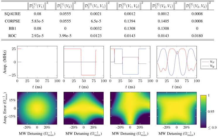
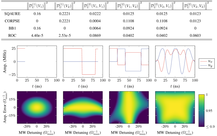
Figure 4: Results for $R_{0}(\pi/2)$. Comparison of: magnitudes of directional derivatives up to second order, pulse shapes, and robustness profiles. From left to right are SQUARE, CORPSE, BB1, and ROC, respectively.

Figure 5: Results for $R_{0}(\pi)$. Comparison of: magnitudes of directional derivatives up to second order, pulse shapes, and robustness profiles. From left to right are SQUARE, CORPSE, BB1, and ROC, respectively.

II.3 Differential Evolution Algorithm

As a powerful global optimization algorithm, differential evolution (DE) [66] has found many successful applications in quantum control problems [67, 68, 69, 70]. Here, we suggest DE as a promising candidate for seeking robust optimal pulses. The parameterized piecewise constant shaped pulse is usually expressed as a vector $u$, called individual in the DE context. The goal is then to maximize the above control fitness function $\Phi(u)$ over $u$. DE functions by performing mutation, crossover and selection operations in the population space which consists of a set of individuals. The algorithm procedure can be described as follows:

Step 1: Set the algorithm constants: scaling factor $R$, crossover rate $C_{r}$, chromosome length (the dimension of each individual) $p$ and population size $P_{s}$. Generate an initial population $P=\{u_{1},...,u_{P_{s}}\}$ randomly with $u_{i}=(u_{i1},...,u_{ip})$ being the $i$-th individual in current population.

Step 2: From $i=1$ to $P_{s}$, do the following steps:

1. Mutation. Generate a donor vector $v_{i}=(v_{i1},...,v_{ip})$ through the mutation rule: ${v_{i}}={u_{r_{b}^{i}}}+R({u_{r_{1}^{i}}}-{u_{r_{2}^{i}}}+{u_{r_{3}^{i}}}-{u_{r_{4}^{i}}}),$ where $r_{1}^{i},r_{2}^{i},r_{3}^{i},r_{4}^{i}$ are randomly chosen mutually exclusive integers in the range $[0,P_{s}]$ and $r_{b}^{i}$ is the index of the best individual in the current population.

2. Crossover. Generate a trial vector $\mu_{i}=(\mu_{i1},...,\mu_{ip})$ by a binomial crossover strategy: if $\text{rand}_{i,j}[0,1]\leq C_{r}$ or $j=j_{\text{rand}}$, let $\mu_{ij}=v_{ij}$, where $j_{\text{rand}}\in\{1,2,...,p\}$ is a randomly chosen index. Otherwise let $\mu_{ij}=u_{ij}$.

3. Selection. Evaluate the former individual $u_{i}$ and the trail vector $\mu_{i}$, if $\Phi(\mu_{i})\geq\Phi(u_{i})$, let $u_{i}=\mu_{i}$, otherwise keep $u_{i}$ unchanged.

Step 3: Check the stopping criterion, if not satisfied, continue with Step 2.

II.4 Results: Comparison with Composite Pulses

Here, we compare the robustness to detuning errors and control amplitude errors between SQUARE, CORPSE, BB1, and our ROC pulses. CORPSE and BB1 are two commonly used composite pulses defined by:

CORPSE: $$R_{0}(\theta)=R_{0}(\theta/2-\theta^{\prime})R_{\pi}(2\pi-2\theta^{\prime})R_{0}(2\pi+\theta/2-\theta^{\prime})$$

BB1: $$R_{0}(\theta)=R_{\phi^{\prime}}(\pi)R_{3\phi^{\prime}}(2\pi)R_{\phi^{\prime}}(\pi)R_{0}(\theta)$$

where $\theta^{\prime}=\arcsin[\sin(\theta/2)/2]$, $\phi^{\prime}=\arccos(-\theta/4\pi)$ We focus on two rotational operations $R_{0}(\pi/2)$ and $R_{0}(\pi)$. The results are presented in Fig. 5 and in Fig. 5.

III Robust DD: Application Examples

III.1 Quantum Identity

The target is the identity operation. We compare between a number of robust DD sequences that employ different basic pulses and different phase modulation strategies. Two phase modulation strategies are considered here:

1. The XY8 sequence XYXYYXYX.

2. The universally robust (UR) DD Sequence proposed in Ref. [23]. UR DD sequence consists a sequel of $n$ equally separated phased pulses. According to [23], the phases of a UR sequence of $n$ pulses is given by

   $$\phi_{k}^{(n)}=\frac{(k-1)(k-2)}{2}\Phi^{(n)}+(k-1)\phi_{2},$$

   where $\Phi^{(4m)}=\pm\pi/m$, and $\Phi^{(4m+2)}=\pm(2m\pi)/(2m+1)$.

The results are as follows:

Here, the control errors are measured in terms of the maximum Rabi frequency $\Omega_{\max}$. All DD sequences contain $N=100$ cycles and have equal total time length of 3.2 ms. From the figure, we clearly see that

1. for the same basic pulse, UR8 outperforms XY8;

2. for the same phase modulation strategy, our ROC pulse performs best.

III.2 Detection of Nuclear Spins

III.2.1 Basic principles and representative detection sequences

In NV center system, through applying a subtle multipulse DD sequence on the electron spin, the weak signal of a specific nuclear spin can be amplified, meanwhile all the other nuclear spins can be dynamically decoupled from the central electron spin. As such, we can resolve and coherently control the nuclear spins. Specifically, the electron spin is firstly prepared at $\rho=|+\rangle\langle+|$ with $|+\rangle=(|0\rangle+|1\rangle)/\sqrt{2}$ and a DD sequence then follows. Finally, the resultant electron spin state $\rho_{t}$ is attached a $R_{\pi/2}(\pi/2)$ rotation and measured in the basis $|0\rangle$, thus we can obtain the transition probability $P=\text{Tr}(\rho_{f}|0\rangle\langle 0|)$. Explicitly, this procedure can be described as:

$$|0\rangle\langle 0|\xRightarrow{R_{\pi/2}(\pi/2)}|+\rangle\langle+|\xRightarrow{\text{DD}}\rho_{t}\xRightarrow{R_{\pi/2}(\pi/2)}\rho_{f}~{}{\Longrightarrow}~{}\text{Tr}(\rho_{f}|0\rangle\langle 0|).$$ (14)

Consider the basic 8-pulse DD unit in ideal case:

$$\frac{\tau}{2}-R_{\phi_{1}}(\pi)-\tau-R_{\phi_{2}}(\pi)-\tau-R_{\phi_{3}}(\pi)-\tau-R_{\phi_{4}}(\pi)-\tau-R_{\phi_{5}}(\pi)-\tau-R_{\phi_{6}}(\pi)-\tau-R_{\phi_{7}}(\pi)-\tau-R_{\phi_{8}}(\pi)-\frac{\tau}{2},$$ (15)

where $R_{\phi_{k}}(\pi)$ represents a $\pi$ rotation around the axis $S_{\phi_{k}}=\cos(\phi_{k})S_{x}+\sin(\phi_{k})S_{y}$. When the interpulse delay $\tau=k\pi/\omega_{I}$ ($k$ is odd number), the corresponding nuclear spin with effective Larmor frequency $\omega_{I}$ can induce a sharp resonant dip in the observed signal (time domain) [13]. This basic unit is usually cycled $L$ times to enhance the signal. The position and amplitude of the dip are then used to infer the hyperfine couplings between the electron spin and the sensed nuclear spin. Equivalently, we can transform this signal to frequency domain, i.e., a sharp resonant peak with detection frequency $\omega=\omega_{I}/k$, for clearly acquiring the spectrum information.

In realistic case, many common pulse imperfections can severely hinder the detection process. Finite width of the $\pi$ pulses, marked as $t_{\pi}$, will shift the resonant positions to $\tau^{\prime}=k\pi/\omega_{I}-t_{\pi}/2$. Detuning and pulse amplitude error can cause spurious peaks and distortion of the baseline. Thus, robust DD sequences that can resist these pulse imperfections are highly demand. In this work, we consider the following representative DD sequences ($\Omega_{\max}=25~{}$MHz).

(1) XY8 sequence. The phases of the basic pulses are $\phi^{\text{XY8}}_{k}=\{0,\pi/2,0,\pi/2,\pi/2,0,\pi/2,0\}$. The resonant positions are $\tau^{\prime}=k\pi/\omega_{I}-t_{\pi}/2$ with $t_{\pi}=20~{}$ns.

(2) UR8 sequence [23]. The phases of the basic pulses are $\phi_{k}^{\text{UR8}}=\{0,\pi/2,3\pi/2,\pi,\pi,3\pi/2,\pi/2,0\}$. The resonant positions are $\tau^{\prime}=k\pi/\omega_{I}-t_{\pi}/2$ with $t_{\pi}=20~{}$ns.

(3) BB1-XY8 sequence [71]. The phases of the basic pulses are $\phi^{\text{BB1-XY8}}_{k}=\{0,\pi/2,0,\pi/2,\pi/2,0,\pi/2,0\}$. Each $R_{\phi_{k}}(\pi)$ is realized by the BB1 composite pulses, namely $R_{\phi_{k}}(\pi)=\Pi_{i=1}^{4}R_{\phi_{i}}(\theta_{i})$ with $\theta_{1}=\theta_{3}=\pi,\theta_{2}=2\pi,\theta_{4}=\pi;\phi_{1}=\phi_{3}=\phi_{k}+\text{accos}(-1/4),\phi_{2}=3\phi_{1}-2\phi_{k},\phi_{4}=\phi_{k}$. The resonant positions then become $\tau^{\prime}=k\pi/\omega_{I}-t_{\text{BB1}}/2$ with $t_{\text{BB1}}=5t_{\pi}=100~{}$ns.

(4) RP-XY8 sequence [24]. The phases of the basic pulses are $\phi_{k}^{\text{RP-XY8}}=\phi^{\text{XY8}}_{k}+\phi_{n},\phi_{n}\in\text{rand}[0,2\pi],n=1,2,...,N$. That is, the 8 basic pulses in each unit are attached a random global phase. The resonant positions are $\tau^{\prime}=k\pi/\omega_{I}-t_{\pi}/2$ with $t_{\pi}=20~{}$ns.

(5) GAXY8 sequence [50]. The phases of the basic pulses are $\phi^{\text{GAXY8}}_{k}=\{0,\pi/2,0,\pi/2,\pi/2,0,\pi/2,0\}$. Each basic $\pi$ rotation is then realized by the 5-pulse composite AXY8 sequence [48]. Further, each AXY8 sequence employs a different amplitude but keeps the same in a DD unit. In this way, the soft modulation can be resembled as the Gaussian shape $\lambda(t)=\lambda_{0}\exp\left[-t^{2}/\left(2\sigma^{2}\right)\right]$ by the sequence of hard $\pi$ pulses, we set $\sigma=T/(4\sqrt{2})$ with $\lambda_{0}=0.271,T=4L\tau$. The resonant positions are $\tau^{\prime}=k\pi/\omega_{I}-t_{\text{AXY8}}$ with $t_{\text{AXY8}}=5t_{\pi}=100~{}$ns.

III.2.2 Searching robust optimal pulses for improving DD robustness

As mentioned above, a multipulse DD sequence can select the signal of a specific nuclear spin, meanwhile dynamically decouple the other nuclear spins. Thus, a system consists of the central electron spin and one target nuclear spin is sufficient to characterize the issue in multi-spin case. For designing robust optimal pulses, we consider the commonly encountered pulse imperfections, including detuning, amplitude error, and finite width of $\pi$ and $\pi/2$ rotations. These factors are treated as perturbations, resulting in the perturbed Hamiltonian

$$H(t)=\Omega_{I}I_{z}+A_{zz}S_{z}I_{z}+A_{zx}S_{x}I_{z}+(1+\epsilon_{\Omega})\Omega(t)[S_{x}\cos(\varphi(t))+S_{y}\sin(\varphi(t))]+\epsilon_{z}\Delta_{\max}S_{z}.$$ (16)

Compared to its general form $H(t)=H_{SE}+H_{C}(u(t))+\sum_{i}\epsilon_{i}V_{i}(t)$, we have $H_{SE}=\Omega_{I}I_{z}+A_{zz}S_{z}I_{z}+A_{zx}S_{x}I_{z},H_{C}(u(t))=\Omega(t)[S_{x}\cos(\varphi(t))+S_{y}\sin(\varphi(t))],V_{1}=\Delta_{\max}S_{z},V_{2}(t)=\Omega(t)[S_{x}\cos(\varphi(t))+S_{y}\sin(\varphi(t))],\varepsilon_{1}=\epsilon_{z},\varepsilon_{2}=\epsilon_{\Omega}$. In our simulations, we concern the case with relatively large pulse imperfections, thus set $\varepsilon_{z}=\varepsilon_{\Omega}=0.08,\Delta_{\max}=\Omega_{\max}=25~{}$MHz. Besides, though we do not know the hyperfine couplings before detection, we can bound them by certain upper values. As such, we set $A_{zz}=A_{zx}\leq 0.1\Omega_{I}$ with $\Omega_{I}=\gamma_{I}B,\gamma_{I}=2\pi\times 1.071~{}$kHz/G, $B=400~{}$G.

In convenience, the time-varied controls $u(t)=(u_{x}(t),u_{y}(t))=(\Omega(t)\cos(\varphi(t)),\Omega(t)\sin(\varphi(t))):t\in[0,\tau_{u}]$ are divided into $M$ piecewise constant slices with equal duration time $\Delta t=\tau_{u}/M$. This transforms the controls into the form $\bm{u}=(u[m])=(u_{x}[m],u_{y}[m]):m\in[1,M]$. For a $\theta$ rotation with a phase shift $\phi$ in DD sequence, i.e., $R_{\phi}(\theta)=e^{-i\theta[\cos(\phi)S_{x}+\sin(\phi)S_{y}]}$, the actual evolution operator can be calculated by

$$U_{\theta,\phi}=\Pi_{m=1}^{M}e^{-i\Delta t\{\Omega_{I}I_{z}+A_{zz}S_{z}I_{z}+A_{zx}S_{x}I_{z}+(1+\epsilon_{\Omega})[u_{x}[m]S_{x}+u_{y}[m]S_{y}]+\epsilon_{z}\Delta_{\max}S_{z}\}}.$$ (17)

By denoting the main physical goal $f_{0}=\text{Tr}(U_{\theta,\phi}R^{\dagger}_{\phi}(\theta))$ and the norm of the corresponding directional derivatives $f_{1}=||\mathcal{D}^{(1)}_{U_{\theta,\phi}}(V_{1})||^{2},f_{2}=||\mathcal{D}^{(1)}_{U_{\theta,\phi}}(V_{2})||^{2},f_{3}=||\mathcal{D}^{(1)}_{U_{\theta,\phi}}(H_{SE})||^{2},f_{4}=||\mathcal{D}^{(2)}_{U_{\theta,\phi}}(V_{1})||^{2},f_{5}=||\mathcal{D}^{(2)}_{U_{\theta,\phi}}(V_{2})||^{2},f_{6}=||\mathcal{D}^{(2)}_{U_{\theta,\phi}}(H_{SE})||^{2}$, the multi-objective control fitness function can be formalized as $\Psi=p_{0}f_{0}+\sum_{i=1}^{6}p_{i}(1-\alpha_{i}f_{i})$. The parameters are carefully tuned and chosen as $p_{0}=1/2,p_{i}=1/12,\alpha_{1}=10^{2},\alpha_{2}=\alpha_{3}=10^{3},\alpha_{4}=10^{4},\alpha_{5}=\alpha_{6}=10^{5}$. According to the ROC procedure using DE algorithm (the algorithm parameters are set as $R=0.6,C_{r}=0.95,p=80,P_{s}=60$, the optimization stops when the control performance function reaches 0.999 within 1000 iterations), the robust optimal pulses can be found, as shown in Fig. 6. Incorporating these robust pulses into the investigated DD sequences can substantially enhance their robustness, as analyzed in the main text.

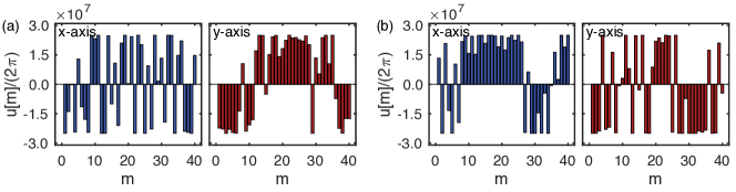
Figure 6: The robust optimal pulses searched by differential evolution algorithm. The pulses are divided into 40 piecewise-constant slices along $x$ and $y$ axes with a total pulse length being $80~{}$ns. (a) The pulses for $R_{\pi/2}(\pi/2)$ rotation. (b) The pulses for $R_{0}(\pi)$ rotation.

III.2.3 Simulation details

We supplement some details and explanations of Fig. 2 in the main text.

Single spin.–The hyperfine couplings and the effective Larmor frequency for the investigated single spin (Fig. 2(a) in the main text) are $A_{zz}^{1}=2\pi\times 27~{}$kHz, $A_{zx}^{1}=2\pi\times 17~{}$kHz, $\omega_{I}=2\pi\times 428.41~{}$kHz. As analyzed, the $k$th order resonant peak appears at location $\omega_{I}/k$ with $k$ being odd. For brevity, we only show the resonant peaks up to third order.

Six spins.–The detailed coupling constants between the NV electron spin and the surrounding six nuclear spins (Fig. 2(b) in the main text) are listed in Table. 1. For brevity, we look over the spectra range that contains all the eighth order resonant peaks of the six spins. It worth noting that when the cycle number $L$ is much larger, the spectrum using the XY8 sequence will be more miscellaneous, while combing our robust optimal pulses can still resist the considered pulse imperfections well.

Spin	$A_{zz}^{n}$ (kHz)	$A_{zx}^{n}$ (kHz)	$\omega^{n}_{I}$ (kHz)	Spin	$A_{zz}^{n}$ (kHz)	$A_{zx}^{n}$ (kHz)	$\omega^{n}_{I}$ (kHz)
1	$2\pi\times 78.234$	$2\pi\times 30.031$	$2\pi\times 468.59$	4	-$2\pi\times 12.958$	$2\pi\times 13.896$	$2\pi\times 422.99$
2	$2\pi\times 40.703$	$2\pi\times 23.500$	$2\pi\times 449.82$	5	-$2\pi\times 22.081$	$2\pi\times 24.525$	$2\pi\times 418.43$
3	$2\pi\times 32.328$	$2\pi\times 44.496$	$2\pi\times 445.64$	6	$2\pi\times 15.796$	$2\pi\times 19.506$	$2\pi\times 437.37$

Table 1: The hyperfine couplings and the effective Larmor frequency for the six nuclear spins derived from Ref. [13]. The Larmor frequency for each nuclear spin is $\Omega_{I}=\gamma_{I}B$ with $\gamma_{I}=2\pi\times 1.071~{}$kHz/G and $B=401~{}$G.

Two close spins.–In Fig. 2(c) in the main text, we use two spectrally close spins with couplings $A_{zz}^{1}=2\pi\times 27.02~{}$kHz, $A_{zx}^{1}=2\pi\times 16.91~{}$kHz, $\omega_{I}^{1}=2\pi\times 441.91~{}$kHz $A_{zz}^{2}=2\pi\times 18.28~{}$kHz, $A_{zx}^{2}=2\pi\times 54.26~{}$kHz, and $\omega_{I}^{2}=2\pi\times 437.53~{}$kHz. As described above, we use the optimal pulses that can minimize the norm of the directional derivatives with respect to the considered imperfections up to the second order. When applying higher order minimizations, we anticipate that the visible gap between our results and the ideal spectrum can be gradually bridged.

References

- Suter and Álvarez [2016] D. Suter and G. A. Álvarez, Colloquium: Protecting quantum information against environmental noise, Rev. Mod. Phys. 88, 041001 (2016).
- Viola et al. [1999] L. Viola, E. Knill, and S. Lloyd, Dynamical Decoupling of Open Quantum Systems, Phys. Rev. Lett. 82, 2417 (1999).
- Du et al. [2009] J. Du, X. Rong, N. Zhao, Y. Wang, J. Yang, and R. B. Liu, Preserving electron spin coherence in solids by optimal dynamical decoupling, Nautre 461, 1265 (2009).
- Biercuk et al. [2009] M. J. Biercuk, H. Uys, A. P. VanDevender, N. Shiga, W. M. Itano, and J. J. Bollinger, Optimized dynamical decoupling in a model quantum memory, Nautre 458, 996 (2009).
- de Lange et al. [2010] G. de Lange, Z. H. Wang, D. Ristè, V. V. Dobrovitski, and R. Hanson, Universal dynamical decoupling of a single solid-state spin from a spin bath, Sciene 330, 60 (2010).
- Zhong et al. [2015] M. Zhong, M. P. Hedges, R. L. Ahlefeldt, J. G. Bartholomew, S. E. Beavan, S. M.Wittig, J. J. Longdell, and M. J. Sellars, Optically addressable nuclear spins in a solid with a six-hour coherence time, Nature 517, 177 (2015).
- West et al. [2010] J. R. West, D. A. Lidar, B. H. Fong, and M. F. Gyure, High Fidelity Quantum Gates via Dynamical Decoupling, Phys. Rev. Lett. 105, 230503 (2010).
- Liu et al. [2013] G.-Q. Liu, H. C. Po, J. Du, R.-B. Liu, and X.-Y. Pan, Noise-resilient quantum evolution steered by dynamical decoupling, Nat. Commun. 4, 2254 (2013).
- Piltz et al. [2013] C. Piltz, B. Scharfenberger, A. Khromova, A. F. Varón, and C. Wunderlich, Protecting Conditional Quantum Gates by Robust Dynamical Decoupling, Phys. Rev. Lett. 110, 200501 (2013).
- Zhang and Suter [2015] J. Zhang and D. Suter, Experimental Protection of Two-Qubit Quantum Gates against Environmental Noise by Dynamical Decoupling, Phys. Rev. Lett. 115, 110502 (2015).
- Bylander et al. [2011] J. Bylander, S. Gustavsson, F. Yan, F. Yoshihara, K. Harrabi, G. Fitch, D. G. Cory, Y. Nakamura, J.-S. Tsai, and W. D. Oliver, Noise spectroscopy through dynamical decoupling with a superconducting flux qubit, Nat. Phys. 7, 565 (2011).
- Álvarez and Suter [2011] G. A. Álvarez and D. Suter, Measuring the Spectrum of Colored Noise by Dynamical Decoupling, Phys. Rev. Lett. 107, 230501 (2011).
- Taminiau et al. [2012] T. H. Taminiau, J. J. T. Wagenaar, T. van der Sar, F. Jelezko, V. V. Dobrovitski, and R. Hanson, Detection and control of individual nuclear spins using a weakly coupled electron spin, Phys. Rev. Lett. 109, 137602 (2012).
- Lang et al. [2015] J. E. Lang, R. B. Liu, and T. S. Monteiro, Dynamical-Decoupling-Based Quantum Sensing: Floquet Spectroscopy, Phys. Rev. X 5, 041016 (2015).
- Abobeih et al. [2019] M. Abobeih, J. Randall, C. Bradley, H. Bartling, M. Bakker, M. Degen, M. Markham, D. Twitchen, and T. Taminiau, Atomic-scale imaging of a 27-nuclear-spin cluster using a quantum sensor, Nature 576, 411 (2019).
- Souza et al. [2012] A. M. Souza, G. A. Álvarez, and D. Suter, Robust dynamical decoupling, Phil. Trans. R. Soc. A 370, 4748 (2012).
- Maudsley [1986] A. A. Maudsley, Modified Carr-Purcell-Meiboom-Gill Sequence for NMR Fourier Imaging Applications, J. Magn. Reson. 69, 488 (1986).
- Viola and Knill [2003] L. Viola and E. Knill, Robust Dynamical Decoupling of Quantum Systems with Bounded Controls, Phys. Rev. Lett. 90, 037901 (2003).
- Khodjasteh and Viola [2009] K. Khodjasteh and L. Viola, Dynamically Error-Corrected Gates for Universal Quantum Computation, Phys. Rev. Lett. 102, 080501 (2009).
- Levitt [1986] M. H. Levitt, Composite pulses, Prog. Nucl. Magn. Reson. Spectrosc. 18, 61 (1986).
- Khodjasteh and Lidar [2005] K. Khodjasteh and D. A. Lidar, Fault-Tolerant Quantum Dynamical Decoupling, Phys. Rev. Lett. 95, 180501 (2005).
- Souza et al. [2011] A. M. Souza, G. A. Álvarez, and D. Suter, Robust Dynamical Decoupling for Quantum Computing and Quantum Memory, Phys. Rev. Lett. 106, 240501 (2011).
- Genov et al. [2017] G. T. Genov, D. Schraft, N. V. Vitanov, and T. Halfmann, Arbitrarily Accurate Pulse Sequences for Robust Dynamical Decoupling, Phys. Rev. Lett. 118, 133202 (2017).
- Wang et al. [2019] Z.-Y. Wang, J. E. Lang, S. Schmitt, J. Lang, J. Casanova, L. McGuinness, T. S. Monteiro, F. Jelezko, and M. B. Plenio, Randomization of Pulse Phases for Unambiguous and Robust Quantum Sensing, Phys. Rev. Lett. 122, 200403 (2019).
- Preskill [2018] J. Preskill, Quantum Computing in the NISQ era and beyond, Quantum 2, 79 (2018).
- Cummins et al. [2003] H. K. Cummins, G. Llewellyn, and J. A. Jones, Tackling systematic errors in quantum logic gates with composite rotations, Phys. Rev. A 67, 042308 (2003).
- Wimperis [1994] S. Wimperis, Broadband, Narrowband, and Passband Composite Pulses for Use in Advanced NMR Experiments, J. Magn. Reson. A 109, 221 (1994).
- Bando et al. [2013] M. Bando, T. Ichikawa, Y. Kondo, and M. Nakahara, Concatenated Composite Pulses Compensating Simultaneous Systematic Errors, J. Phys. Soc. Jpn. 82, 014004 (2013).
- Werschnik and Gross [2007] J. Werschnik and E. K. U. Gross, Quantum optimal control theory, J. Phys. B: At. Mol. Opt. Phys. 40, R175 (2007).
- Haas et al. [2019] H. Haas, D. Puzzuoli, F. Zhang, and D. G. Cory, Engineering effective Hamiltonians, New. J. Phys. 21, 103011 (2019).
- Kolkowitz et al. [2012] S. Kolkowitz, Q. P. Unterreithmeier, S. D. Bennett, and M. D. Lukin, Sensing Distant Nuclear Spins with a Single Electron Spin, Phys. Rev. Lett. 109, 137601 (2012).
- London et al. [2013] P. London, J. Scheuer, J.-M. Cai, I. Schwarz, A. Retzker, M. B. Plenio, M. Katagiri, T. Teraji, S. Koizumi, J. Isoya, R. Fischer, L. P. McGuinness, B. Naydenov, and F. Jelezko, Detecting and Polarizing Nuclear Spins with Double Resonance on a Single Electron Spin, Phys. Rev. Lett. 111, 067601 (2013).
- Pla et al. [2012] J. J. Pla, K. Y. Tan, J. P. Dehollain, W. H. Lim, J. J. Morton, D. N. Jamieson, A. S. Dzurak, and A. Morello, A single-atom electron spin qubit in silicon, Nature 489, 541 (2012).
- Morton et al. [2008] J. J. Morton, A. M. Tyryshkin, R. M. Brown, S. Shankar, B. W. Lovett, A. Ardavan, T. Schenkel, E. E. Haller, J. W. Ager, and S. Lyon, Solid-state quantum memory using the 31p nuclear spin, Nature 455, 1085 (2008).
- Schlipf et al. [2017] L. Schlipf, T. Oeckinghaus, K. Xu, D. B. R. Dasari, A. Zappe, F. F. de Oliveira, B. Kern, M. Azarkh, M. Drescher, M. Ternes, K. Kern, J. Wrachtrup, and A. Finkler, A molecular quantum spin network controlled by a single qubit, Sci. Adv. 3, e1701116 (2017).
- Ajoy et al. [2019] A. Ajoy, U. Bissbort, D. Poletti, and P. Cappellaro, Selective Decoupling and Hamiltonian Engineering in Dipolar Spin Networks, Phys. Rev. Lett. 122, 013205 (2019).
- Lidar and Todd A. Brun [2013] D. A. Lidar and e. Todd A. Brun, Quantum Error Correction (Cambridge University Press, Cambridge, England, 2013).
- [38] See Supplemental Material for more details.
- Dyson [1949] F. J. Dyson, The Radiation Theories of Tomonaga, Schwinger, and Feynman, Phys. Rev. 75, 486 (1949).
- Wang et al. [2020] Z. Wang, J. Casanova, and M. B. Plenio, Enhancing the robustness of dynamical decoupling sequences with correlated random phases, Symmetry 12, 730 (2020).
- Loretz et al. [2015] M. Loretz, J. M. Boss, T. Rosskopf, H. J. Mamin, D. Rugar, and C. L. Degen, Spurious harmonic response of multipulse quantum sensing sequences, Phys. Rev. X 5, 021009 (2015).
- Khaneja et al. [2005a] N. Khaneja, T. Reiss, C. Kehlet, T. Schulte-Herbrüggen, and S. J. Glaser, Optimal control of coupled spin dynamics: design of NMR pulse sequences by gradient ascent algorithms, J. Magn. Reson. 172, 296 (2005a).
- Palittapongarnpim et al. [2017] P. Palittapongarnpim, P. Wittek, E. Zahedinejad, S. Vedaie, and B. C. Sanders, Learning in quantum control: High-dimensional global optimization for noisy quantum dynamics, Neurocomputing 268, 116 (2017).
- Dong et al. [2020] D. Dong, X. Xing, H. Ma, C. Chen, Z. Liu, and H. Rabitz, Learning-Based Quantum Robust Control: Algorithm, Applications, and Experiments, IEEE Trans. Cybern. 50, 3581 (2020).
- Zahedinejad et al. [2015a] E. Zahedinejad, J. Ghosh, and B. C. Sanders, High-Fidelity Single-Shot Toffoli Gate via Quantum Control, Phys. Rev. Lett. 114, 200502 (2015a).
- Ladd et al. [2010] T. D. Ladd, F. Jelezko, R. Laflamme, Y. Nakamura, C. Monroe, and J. L. O’Brien, Quantum computers, Nature 464, 45 (2010).
- Bradley et al. [2019] C. E. Bradley, J. Randall, M. H. Abobeih, R. C. Berrevoets, M. J. Degen, M. A. Bakker, M. Markham, D. J. Twitchen, and T. H. Taminiau, A Ten-Qubit Solid-State Spin Register with Quantum Memory up to One Minute, Phys. Rev. X 9, 031045 (2019).
- Casanova et al. [2015] J. Casanova, Z.-Y. Wang, J. F. Haase, and M. B. Plenio, Robust dynamical decoupling sequences for individual-nuclear-spin addressing, Phys. Rev. A 92, 042304 (2015).
- Casanova et al. [2016] J. Casanova, Z.-Y. Wang, and M. B. Plenio, Noise-Resilient Quantum Computing with a Nitrogen-Vacancy Center and Nuclear Spins, Phys. Rev. Lett. 117, 130502 (2016).
- Haase et al. [2018] J. F. Haase, Z.-Y. Wang, J. Casanova, and M. B. Plenio, Soft quantum control for highly selective interactions among joint quantum systems, Phys. Rev. Lett. 121, 050402 (2018).
- Rej et al. [2015] E. Rej, T. Gaebel, T. Boele, D. E. Waddington, and D. J. Reilly, Hyperpolarized nanodiamond with long spin-relaxation times, Nat. Commu. 6, 8459 (2015).
- Scheuer et al. [2017] J. Scheuer, I. Schwartz, S. Müller, Q. Chen, I. Dhand, M. B. Plenio, B. Naydenov, and F. Jelezko, Robust techniques for polarization and detection of nuclear spin ensembles, Phys. Rev. B 96, 174436 (2017).
- Henstra et al. [1988] A. Henstra, P. Dirksen, J. Schmidt, and W. Wenckebach, Nuclear spin orientation via electron spin locking (NOVEL), J. Mag. Reson. 77, 389 (1988).
- Chen et al. [2015] Q. Chen, I. Schwarz, F. Jelezko, A. Retzker, and M. B. Plenio, Optical hyperpolarization of nuclear spins in nanodiamond ensembles, Phys. Rev. B 92, 184420 (2015).
- Scheuer et al. [2016] J. Scheuer, I. Schwartz, Q. Chen, D. Schulze-Sünninghausen, P. Carl, P. Höfer, A. Retzker, H. Sumiya, J. Isoya, B. Luy, M. B. Plenio, B. Naydenov, and F. Jelezko, Optically induced dynamic nuclear spin polarisation in diamond, New J. Phys. 18, 013040 (2016).
- Schwartz et al. [2018] I. Schwartz, J. Scheuer, B. Tratzmiller, S. Müller, Q. Chen, I. Dhand, Z.-Y. Wang, C. Müller, B. Naydenov, F. Jelezko, and M. B. Plenio, Robust optical polarization of nuclear spin baths using Hamiltonian engineering of nitrogen-vacancy center quantum dynamics, Sci. Adv. 4, eaat8978 (2018).
- Denning et al. [2019] E. V. Denning, D. A. Gangloff, M. Atatüre, J. Mørk, and C. Le Gall, Collective Quantum Memory Activated by a Driven Central Spin, Phys. Rev. Lett. 123, 140502 (2019).
- Pagliero et al. [2020] D. Pagliero, P. R. Zangara, J. Henshaw, A. Ajoy, R. H. Acosta, J. A. Reimer, A. Pines, and C. A. Meriles, Optically pumped spin polarization as a probe of many-body thermalization, Sci. Adv. 6, eaaz6986 (2020).
- Lovchinsky et al. [2017] I. Lovchinsky, J. Sanchez-Yamagishi, E. Urbach, S. Choi, S. Fang, T. Andersen, K. Watanabe, T. Taniguchi, A. Bylinskii, E. Kaxiras, P. Kim, H. Park, and M. D. Lukin, Magnetic resonance spectroscopy of an atomically thin material using a single-spin qubit, Science 355, 503 (2017).
- Schmid-Lorch et al. [2015] D. Schmid-Lorch, T. Häberle, F. Reinhard, A. Zappe, M. Slota, L. Bogani, A. Finkler, and J. Wrachtrup, Relaxometry and Dephasing Imaging of Superparamagnetic Magnetite Nanoparticles Using a Single Qubit, Nano Lett. 15, 4942 (2015).
- Barends et al. [2014] R. Barends, J. Kelly, A.Megrant, A. Veitia, D.Sank, E. Jeffrey, T. C.White, J. Mutus, A. G. Fowler, B. Campbell, Y. Chen, Z. Chen, B. Chiaro, A. Dunsworth, C. Neill, P. O’Malley, P. Roushan, A. Vainsencher, J. Wenner, A. N. Korotkov, A. N. Cleland, and J. M. Martinis, Superconducting quantum circuits at the surface code threshold for fault tolerance, Nature 508, 500 (2014).
- Reagor et al. [2018] M. Reagor, C. B. Osborn, N. Tezak, A. Staley, G. Prawiroatmodjo, M. Scheer, N. Alidoust, E. A. Sete, N. Didier, M. P. da Silva, E. Acala, J. Angeles, A. Bestwick, M. Block, B. Bloom, A. Bradley, C. Bui, S. Caldwell, L. Capelluto, R. Chilcott, J. Cordova, G. Crossman, M. Curtis, S. Deshpande, T. El Bouayadi, D. Girshovich, S. Hong, A. Hudson, P. Karalekas, K. Kuang, M. Lenihan, R. Manenti, T. Manning, J. Marshall, Y. Mohan, W. O’Brien, J. Otterbach, A. Papageorge, J.-P. Paquette, M. Pelstring, A. Polloreno, V. Rawat, C. A. Ryan, R. Renzas, N. Rubin, D. Russel, M. Rust, D. Scarabelli, M. Selvanayagam, R. Sinclair, R. Smith, M. Suska, T.-W. To, M. Vahidpour, N. Vodrahalli, T. Whyland, K. Yadav, W. Zeng, and C. T. Rigetti, Demonstration of universal parametric entangling gates on a multi-qubit lattice, Sci. Adv. 4, eaao3603 (2018).
- Soare et al. [2014] A. Soare, H. Ball, D. Hayes, J. Sastrawan, M. Jarratt, J. McLoughlin, X. Zhen, T. Green, and M. Biercuk, Experimental noise filtering by quantum control, Nat. Phys. 10, 825 (2014).
- Fernández-Acebal et al. [2018] P. Fernández-Acebal, O. Rosolio, J. Scheuer, C. Müller, S. Müller, S. Schmitt, L. McGuinness, I. Schwarz, Q. Chen, A. Retzker, B. Naydenov, F. Jelezko, and M. B. Plenio, Toward Hyperpolarization of Oil Molecules via Single Nitrogen Vacancy Centers in Diamond, Nano Lett. 18, 1882 (2018).
- Khaneja et al. [2005b] N. Khaneja, T. Reiss, C. Kehlet, T. Schulte-Herbrüggen, and S. J.Glaser, Optimal control of coupled spin dynamics: design of nmr pulse sequences by gradient ascent algorithms, J. Magn. Reson. 172, 296 (2005b).
- Das and Suganthan [2011] S. Das and P. N. Suganthan, Differential evolution: A survey of the state-of-the-art, IEEE Trans. Evol. Comput. 15, 4 (2011).
- Zeidler et al. [2001] D. Zeidler, S. Frey, K.-L. Kompa, and M. Motzkus, Evolutionary algorithms and their application to optimal control studies, Phys. Rev. A 64, 023420 (2001).
- Zahedinejad et al. [2015b] E. Zahedinejad, J. Ghosh, and B. C. Sanders, High-fidelity single-shot toffoli gate via quantum control, Phys. Rev. Lett. 114, 200502 (2015b).
- Zahedinejad et al. [2016] E. Zahedinejad, J. Ghosh, and B. C. Sanders, Designing high-fidelity single-shot three-qubit gates: A machine-learning approach, Phys. Rev. Applied 6, 054005 (2016).
- Yang et al. [2019] X. Yang, J. Li, and X. Peng, An improved differential evolution algorithm for learning high-fidelity quantum controls, Sci. Bull. 64, 1402 (2019).
- Brown et al. [2004] K. R. Brown, A. W. Harrow, and I. L. Chuang, Arbitrarily accurate composite pulse sequences, Phys. Rev. A 70, 052318 (2004).