Load Encoding for Learning AC-OPF

Abstract

The AC Optimal Power Flow (AC-OPF) problem is a core building block in electrical transmission system. It seeks the most economical active and reactive generation dispatch to meet demands while satisfying transmission operational limits. It is often solved repeatedly, especially in regions with large penetration of wind farms to avoid violating operational and physical limits. Recent work has shown that deep learning techniques have huge potential in providing accurate approximations of AC-OPF solutions. However, deep learning approaches often suffer from scalability issues, especially when applied to real life power grids. This paper focuses on the scalability limitation and proposes a load compression embedding scheme to reduce training model sizes using a 3-step approach. The approach is evaluated experimentally on large-scale test cases from the PGLib, and produces an order of magnitude improvements in training convergence and prediction accuracy.

I Introduction

The AC Optimal Power Flow (AC-OPF) is an optimization model that finds the most economical generation dispatch meeting the consumer demand, while satisfying the physical and operational constraints of the underlying power network [1]. The AC-OPF, together with its approximations and relaxations, constitutes a fundamental building block for day ahead and real time market operations, including the day-ahead security-constrained unit commitment and real time security-constrained economic dispatch.

The non-convexity of the OPF limits the solving frequency of many operational tools. In practice, generation dispatch in real time markets are often required to be cleared in every couple of minutes. Additionally, the integration of renewable energy and demand response programs create significant stochasticity in load and generation. To improve solving efficiency, recently there has been a growing interest in applying machine learning techniques to power system optimization problems. One line of research focus on how to predict AC-OPF solutions directly using Deep Neural Networks (DNN) (e.g., [2, 3, 4, 5]). Once a deep neural network is trained, predictions can be computed in the order of milliseconds with a single forward pass through the network. Deep neural networks can also be spatially decomposed [6] to learn large-scale power networks.

Prior results are encouraging, showing that deep learning techniques can approximate solutions with high quality. However, many of these learning models tend to have a very large number of input features and training parameters. For deep learning, re-training Deep Neural Nets with a large number of features and parameters is computationally challenging, in particular when generator commitments and grid topology are changing due to operators/market decisions and DNN needs to be frequently updated within the day-ahead/realtime markets. Avoiding re-training completely is also computationally challenging since crafting a generic learning framework on a complex engineering system considering for all possible generator commitments, renewable forecasts, topological changes, and operator decisions is extremely difficult and intractable.

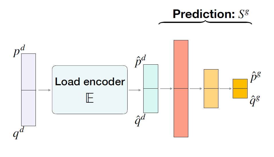
Figure 1: OPF-DNN Training Architecture with Encoder $\mathbb{E}$.

This paper tackles the the scalability issues of deep neural networks for learning AC-OPF when the network scales with increasing load demand input features. Its main contribution is a load embedding scheme that reduces the input feature dimension of the deep learning network. The approach is based on the recognition that, in many circumstances, aggregating loads at adjacent buses does not fundamentally change the nature of the AC-OPF predictions. The load embedding scheme has two key components: (1) An optimization model for load aggregation that reduces the number of loads in an OPF instance, while staying close to the optimal AC-OPF cost; and (2) A learning model for load embedding that, given the loads for an AC-OPF instance, returns a vector of encoded loads of smaller dimensions. It is important to emphasize that the proposed approach is not a generic network reduction technique for preserving the network physical properties. Its goal is to reduce the input feature dimension of the learning model to maintain decent training accuracy within a time limit.

Figure 1 shows the training architecture. The encoder first computes a load embedding, which will then be used as inputs to the learning model to predict the AC-OPF solutions (e.g., active & reactive generator dispatch). The encoder and AC-OPF learning models do not share parameters and are trained in sequence — first learns the encoder and then trains the AC-OPF DNN using the outputs of the learned encoder.

The approach has been evaluated on a wide range of PGLib (formerly NESTA) test cases [7, 8]. Results show that the proposal can produce significant dimensionality reduction and significant improvements in convergence speed and accuracy.

II Related Work

Power network reduction techniques, such as Kron and Ward reduction [9] and Principle Component Anaylsis [10], have been widely used in the industry for more than 70 years. Early techniques focused on crafting simpler equivalent circuits to be used by system operators for analysis. With the advancement of computer technology and lower computation costs, complex reduction models became more feasible [11, 12, 13, 14]. While it is possible to use classical reduction techniques to reduce the power systems before constructing the learning model, the learned model can only predict the reduced networks, with potential accuracy issues. The main focus of the paper is not on general network reduction techniques. Instead, it focuses on reducing the size of the input features and learnable parameters while retaining the prediction accuracy.

Dimension reduction is an important and widely studied topic in machine learning, and reduction techniques have been successfully applied on various learning applications in power systems. For example, auto-encoders have been applied to predict renewable productions [15, 16], and to detect false data injection attacks [17]. The proposed approach differs from general auto-encoder techniques on several aspects. First, the load embeddings are explicitly computed through a bilevel optimization model and not implicitly trained by an auto-encoder. Second, the computed load embeddings are AC-feasible, and their optimal power flows have the same cost as the original ones. Third, the reduced dimensionality is determined by optimization models instead of chosen a-priori.

III Background

This paper uses the rectangular form for complex power $S=p+jq$ and line/transformer admittance $Y=g+jb$, where $p$ and $q$ denote active and reactive powers, and $g$ and $b$ denote conductance and susceptance. Complex voltages are in polar form $V=ve^{j\theta}$, with magnitude $v=\lvert V\rvert$ and phase angle $\theta=\angle V$. Notation $x^{*}$ is used to represent the complex conjugate of quantity $x$ and notation $\hat{x}$ the prediction of quantity $x$.

III-A AC Optimal Power Flow

The AC Optimal Power Flow (OPF) determines the most economical generation dispatch balancing the load and generation in a power network (grid). A power network $\bm{\mathcal{N}}$ is represented as a graph $(N,E)$, where the set of nodes $N$ represent buses and the set of edges $E$ represent branches. Since edges in $E$ are directed, $E^{R}$ is used to denote arcs in the reverse direction. The AC power flow equations are expressed in terms of complex quantities for voltage $V$, admittance $Y$, and power $S$. Model 1 presents an AC OPF formulation, with variables and parameters in the complex domain for ease of presentation. Superscripts $u$ and $l$ are used to indicate upper and lower bounds for variables. The objective function ${\mathcal{O}}(\bm{S^{g}})$ captures the cost of the generator dispatch, with $\bm{S^{g}}$ denoting the vector of generator dispatch values $(S^{g}_{i}\>|\>i\in N)$. Constraint (2) sets the voltage angle of an arbitrary slack bus $s\in N$ to zero to eliminate numerical symmetries. Constraints (3) bound the voltage magnitudes for every bus, and constraints (4) limit the voltage angle differences for every branch. Constraints (5) enforce the generator output $S^{g}_{i}$ to stay within its limits $[S^{gl}_{i},S^{gu}_{i}]$. Constraints (6) impose the line flow limits $s_{ij}^{u}$ on all the line flow variables $S_{ij}$. Constraints (7) capture Kirchhoff’s Current Law enforcing the flow balance of generations $S^{g}_{i}$, loads $S^{d}_{i}$, and branch flows $S_{ij}$ across every node. Finally, constraints (8) capture Ohm’s Law describing the nonlinear and nonconvex AC power flow $S_{ij}$ across lines/transformers.

Model 1 $\mathcal{O}({\bm{S^{d}}})$: AC Optimal Power Flow

input: $$S^{d}_{i}\;\;\forall i\in N$$

variables: $$S^{g}_{i},V_{i}\;\;\forall i\in N,\;\;S_{ij}\;\;\forall(i,j)\in E\cup E^{R}$$

minimize: $$\sum_{i\in N}{c}_{2i}(\Re(S^{g}_{i}))^{2}+{c}_{1i}\Re(S^{g}_{i})+{c}_{0i}$$ (1)

subject to: $$\angle V_{s}=0,\;\;s\in N$$ (2)

$${v}^{l}_{i}\leq|V_{i}|\leq{v}^{u}_{i}\;\;\forall i\in N$$ (3)

$${\theta}^{l}_{ij}\leq\angle(V_{i}V^{*}_{j})\leq{\theta}^{u}_{ij}\;\;\forall(i,j)\in E$$ (4)

$${S}^{gl}_{i}\leq S^{g}_{i}\leq{S}^{gu}_{i}\;\;\forall i\in N$$ (5)

$$|S_{ij}|\leq{s}^{u}_{ij}\;\;\forall(i,j)\in E\cup E^{R}$$ (6)

$$S^{g}_{i}-{S}^{d}_{i}=\textstyle\sum_{(i,j)\in E\cup E^{R}}S_{ij}\;\;\forall i\in N$$ (7)

$$S_{ij}={Y}^{*}_{ij}|V_{i}|^{2}-{Y}^{*}_{ij}V_{i}V^{*}_{j}\;\;\forall(i,j)\in E\cup E^{R}$$ (8)

III-B Deep Learning Models

Deep Neural Networks (DNNs) are learning architectures composed of a sequence of layers, each typically taking as inputs the results of the previous layer. Feed-forward neural networks are DNNs where the layers are fully connected and the function connecting the layers is given by $\bm{y}=\pi(\bm{W}\bm{x}+\bm{b}),$ where $\bm{x}\in\mathbb{R}^{n}$ is an input vector with dimension $n$, $\bm{y}\in\mathbb{R}^{m}$ is the output vector with dimension $m$, $\bm{W}\in\mathbb{R}^{m\times n}$ is a matrix of weights, and $\bm{b}\in\mathbb{R}^{m}$ is a bias vector. Together, $\bm{W}$ and $\bm{b}$ define the trainable parameters of the network. The activation function $\pi$ is usually non-linear (e.g., a rectified linear unit (ReLU)). This paper uses the following OPF-DNN models from  [2] to evaluate the proposed embedding scheme:

$$\bm{h}_{1} =\pi(\bm{W}_{1}\bm{x}+\bm{b}_{1}),\;\;\bm{h}_{2}=\pi(\bm{W}_{2}\bm{h}_{1}+\bm{b}_{2}),$$

$$\bm{y} =\pi(\bm{W}_{3}\bm{h}_{2}+\bm{b}_{3})$$ (9)

where the input vector $\bm{x}=(\bm{p^{d}},\bm{q^{d}})$ represents the vector of active and reactive loads, and the output vector $\bm{y}$ represents the vector of active and reactive generation dispatch predictions $\bm{y}=(\bm{p^{g}},\bm{q^{g}})$. Learning DNN models consists in finding matrices $\bm{W}$, and the associated bias vectors $\bm{b}$, to make the output prediction $\bm{\hat{y}}$ close to the ground truth $\bm{y}$, as measured by a loss function $\mathbb{L}$.

IV Dimensionality Reduction by Load Embedding

This section motivates the concept of load embedding, which is formalized using a bilevel optimization model. The load embedding is motivated by the fact that real-life transmission systems are large and involve tens of thousands of buses and loads. Naively incorporating all the input features of a large system would easily result in a humongous neural network, which is difficult to train and computationally challenging to cope with time limits in practice. The proposed dimensionality reduction is motivated by the observation that, unless there is significant congestion or line power losses, moving a unit of load between two adjacent buses will not have a major effect on the final dispatch. This observation yields opportunities to aggregate load features into smaller subsets and reduce the number of training parameters. This section explores an encoder that performs such an aggregation.

IV-A The Bilevel Load-Embedding Model $\mathcal{M}_{\text{BL}}$

Let $\mathcal{O}^{o}$ be the optimal cost of the original OPF, $S^{g,o}_{i}$ the original dispatch of generator $i$, and $S^{d,o}_{i}=p^{d,o}_{i}+jq^{d,o}_{i}$ the original complex load $i$. The load-embedding model can be formulated as a bilevel optimization model $\mathcal{M}_{\text{BL}}$:

$$\min\;\; \sum_{i\in N}\mathbb{1}{(S^{d}_{i}\neq 0)}$$ (10)

s.t. $$\eqref{eq:ac_0}-\eqref{eq:ac_6}$$ (AC Power Flow) (11)

$$S^{g}_{i}=S^{g,o}_{i}\;\;\forall i\in N,$$ (Generation Equiv.) (12)

$$\sum_{i\in N}p^{d}_{i}=\sum_{i\in N}p^{d,o}_{i}$$ (Active Load Equiv.) (13)

$$\sum_{i\in N}q^{d}_{i}=\sum_{i\in N}q^{d,o}_{i}$$ (Reactive Load Equiv.) (14)

$$\lvert\mathcal{O}(\bm{S^{d}})-\mathcal{O}^{o}\rvert\leq\beta$$ (Cost Equiv.) (15)

Its goal is to find the embedded loads $(p^{d}_{i},q^{d}_{i})$ ($i\in N$) which are the key decision variables. Objective (10) minimizes the number of nonzero loads using an indicator function. Constraints (11) impose the power flow equations. Constraints (12) ensure that the generation dispatch remains the same, given that they are the targets of the learning task. Constraints (13) and (14) require the sum of the active and reactive loads to remain the same after the encoding. Together, these constraints ensure that the loads are AC-feasible for the original generation dispatch. However, they do not guarantee that they could not be served by a significantly better generator dispatch. This is the role of constraint (15) that ensures the encoded load vector $\bm{S^{d}}=\bm{p^{d}}+j\bm{q^{d}}$ induces an optimal flow with cost close to the original cost $\mathcal{O}^{o}$ (within a tolerance parameter $\beta$). This constraint introduces an AC-OPF as a subproblem, hence creating a bilevel model.

IV-B Load Embedding with Congestion Constraints: Model $\mathcal{M}_{\text{R}}$

Optimization model $\mathcal{M}_{\text{BL}}$ is challenging for two reasons: (1) it implicitly features discrete variables through the indicator variables in its objective; (2) it is a bilevel optimization problem. The first challenge can be addressed by replacing its discrete objective by a continuous expression that maximizes the square of the real and reactive powers of each load, i.e.,

$$\max\;\; \sum_{i\in N}[(p^{d}_{i})^{2}+(q^{d}_{i})^{2}].$$ (16)

Objective (16) encourages active and reactive loads to be aggregated without the need of binary variables.

The second challenge can be addressed by replacing constraint (15) by proxy constraints that characterize the OPF. Indeed, in the original OPF, a number of voltage and thermal constraints are binding. Imposing constraints on the associated voltages and flows will help in keeping the optimal cost close to the original cost. Let $N^{l}$ and $N^{u}$ be the set of buses with binding lower and upper constraints on voltages, and $E^{u}$ be the set of lines with binding thermal limit constraints. Constraint (15) can be relaxed and reformulated as:

$$\lvert v_{i}-v^{u}_{i}\rvert\leq\beta_{v},\forall i\in N^{u}$$ (Voltage Congestion) (17)

$$\lvert v_{i}-v^{l}_{i}\rvert\leq\beta_{v},\forall i\in N^{l}$$ (Voltage Congestion) (18)

$$\lvert\lvert S_{ij}\rvert-s^{u}_{ij}\rvert\leq\beta_{s},\forall(i,j)\in E^{u}$$ (Line Congestion) (19)

where $\beta_{v}$ and $\beta_{s}$ are the tolerance parameters for the tightness of the original binding constraints. The relaxed model $\mathcal{M}_{\text{R}}$ is then defined as:

$$\max\;\; \sum_{i\in N}[(p^{d}_{i})^{2}+(q^{d}_{i})^{2}]$$

s.t. $$\eqref{eq:ac_0}-\eqref{eq:ac_6}$$ (AC Power Flow)

$$\eqref{bl_2}-\eqref{bl_4}$$ (Equiv. Constr.)

$$\eqref{r_1}-\eqref{r_3}$$ (Congestion Constr.)

IV-C Load Embedding with a Penalty Method: Model $\mathcal{M}_{\text{P}}$

Model $\mathcal{M}_{\text{R}}$ requires the choice of tolerance parameters $\beta_{v}$ and $\beta_{s}$. If these tolerances are too tight, it may not be possible to aggregate loads effectively. If they are too loose, the resulting predictions may be inaccurate. To overcome this difficulty, this paper uses a penalty method. The resulting model $\mathcal{M}_{\text{P}}(\beta_{v},\beta_{s})$ becomes

$$\max\;\; \sum_{i\in N}[(p^{d}_{i})^{2}+(q^{d}_{i})^{2}]+\beta_{v}\sum_{i\in N^{u}}\lVert v_{i}-v^{u}_{i}\rVert^{2}+$$

$$\beta_{v}\sum_{i\in N^{l}}\lVert v_{i}-v^{l}_{i}\rVert^{2}+\beta_{s}\sum_{(i,j)\in E^{u}}\lVert\lvert S_{ij}\rvert-s^{u}_{ij}\rVert^{2}$$

s.t. $$\eqref{eq:ac_0}-\eqref{eq:ac_6}\mbox{ and }\eqref{bl_2}-\eqref{bl_4}$$

and it can be solved iteratively by increasing $\beta_{v}$ and $\beta_{s}$ until (15) is satisfied, using Algorithm 1.

Input : $\mathcal{N}:$ power grid data; $\rho_{v},\rho_{s}:$ penalty steps;

$(\beta_{v},\beta_{s}):$ constraint tolerances;

$\beta:$ cost tolerance;

$i^{u}:$ max iteration limit.

Output : $\bm{S^{d}}=(\bm{p^{d}},\bm{q^{d}})$

1 for $i=0,1,2,\ldots,i^{u}$ do

2       $\bm{S^{d}}\leftarrow(\bm{p^{d}},\bm{q^{d}})\leftarrow\mathcal{M}_{\text{R}}(\beta_{v},\beta_{s})$

3       if $\lvert\mathcal{O}(\bm{S^{d}})-\mathcal{O}^{o}\rvert\leq\beta$ then

4            break

5      $\beta_{v}\leftarrow\rho_{v}\beta_{v},\;\;\beta_{s}\leftarrow\rho_{s}\beta_{s}$

6      

Algorithm 1 Load Encoding

V Learning to Encode

Algorithm 1 computes an “optimal” load embedding for a load profile $\bm{S^{d}}$. However, computing Algorithm 1 at prediction time is expensive, hence defeating the purpose of speed up OPF computations. Instead, this paper proposes to learn the encoder, i.e., to learn a machine-learning proxy for Algorithm 1. The idea is to take the set of training instances for OPF and apply Algorithm 1 to obtain the load embeddings. The machine-learning model then learns the mapping between the original and embedded loads. The input vector is the load vector $\bm{x}=(\bm{p^{d}},\bm{q^{d}})$ and the output vector is the embedded load vector $\bm{z}=(\bm{\hat{p}^{d}},\bm{\hat{q}^{d}})$. The structure of the output, i.e., the embedded load vector, is obtained by removing the loads that are relocated in all the training instances. The training of the machine-learning model then consists in mapping the original loads into this smaller set of loads to mimic Algorithm 1. The paper proposes to learn the encoder, and explores two learning schemes: (1) a linear regression $\mathbb{E}_{L}(\bm{x})=\bm{z}=\bm{W}\bm{x}+\bm{b},$ that is extremely fast, and; (2) a DNN similar to (9) $\mathbb{E}_{F}(\bm{x})=\bm{z}=\pi\{\bm{W}_{3}\pi[\bm{W}_{2}\pi(\bm{W}_{1}\bm{x}+\bm{b}_{1})+\bm{b}_{2}]+\bm{b}_{3}\}.$

For the full NN-encoder, the dimension of the first and second layers are set to twice of the dimensions of the input and the output vectors respectively. For a data set collection $\mathbb{D}=\{(\bm{x}^{i},\bm{z}^{i}):i\in[1\dotsc n]\}$ with $n$ test cases where the outputs $\bm{z}^{i}$ are computed using Algorithm 1, the goal of the learning task is to find the model parameters $\bm{W}$ and $\bm{b}$ that minimize the empirical risk function:

$$\min_{\bm{W},\bm{b}} \sum_{(\bm{x}^{i},\bm{z}^{i})\in\mathbb{D}}\mathbb{L}(\mathbb{E}_{m}(\bm{x}^{i}),\bm{z}^{i}).$$ (20)

where $m\in\{L,F\}$ is used to discriminate the model adopted.

VI Scalable OPF Learning

Once the load encoder has been learned, the OPF learning task is performed using the architecture in Figure 1. NN layers (tensors) are represented by rectangular boxes and arrows represent connections between layers. The architecture uses fully connected layers with ReLU as the activation functions. Notice that the encoder is pre-trained, so the learning task will not affect its parameters. The dimensions of $h_{1}$ and $h_{2}$ of the OPF layers are set to twice of the dimension of the input and the output vectors respectively as [2].

Unless required to, the encoder does not preserve the values of many physical parameters, including phase angles, voltage magnitudes, and line flows. However, these physical values on the reduced network, which are available as a result of Algorithm 1, are still important to improve prediction accuracy using, for instance, a Lagrangian dual approach as in [2].

VII Experimental Evaluation

Parameter Setup: The experiments were performed on various PGLib (formerly NESTA) test cases [7], and Algorithm 1 was implemented on top of PowerModels.jl [18], a state-of-the-art open source Julia package for solving or approximating AC-OPF. The tolerance $\beta$ was set to 0.5%, $i^{u}=500$, and parameters $\rho_{v}$ and $\rho_{s}$ were both set to 1.5. The OPF data sets were generated by varying the load profiles of each benchmark network from 80% to 120% of their original (complex) load values, with a step size of 0.02%, giving a maximum of 2000 test cases for every benchmark network. For each test case, to create enough diversity, every load is perturbed with random noise from the polar Laplace distribution whose parameter $\lambda$ is set to 10% of the apparent power. The test cases were split with 80%-20% ratio for training and testing. The OPF-DNN models and the encoding models ($\mathbb{E}_{L}/\mathbb{E}_{F}$), were implemented using PyTorch [19] and run with Python 3.6, with the Mean Squared Error (MSE) as the loss function. The training was performed using Tesla-V100 GPUs with 16GBs HBM2 ram on machines with Intel CPU cores at 2.1GHz. The training used Averaged Stochastic Gradient Descent (ASGD) with learning rate $0.001$. The paper uses default parameters from PyTorch for all other hyper-parameters across various learning models.

TABLE I: OPF-DNN: Original & Reduced Input dimension

Network	Orig. dim.	Reduced dim.	Reduction %
14_ieee	22	11	50%
30_ieee	42	13	69%
39_epri	42	29	31%
57_ieee	84	26	69%
73_ieee_rts	102	88	14%
89_pegase	70	55	21%
118_ieee	198	198	0%
162_ieee_dtc	226	143	37%
189_edin	1244	336	73%
1394_sop_eir	524	207	60%
1460_wp_eir	536	536	0%
1888_rte	2000	1555	22%
2848_rte	3022	2310	24%
2868_rte	3102	2221	28%
3012wp_mp	4542	2043	55%
3375wp_mp	4868	2109	57%

VII-A Compression Ratios

Table I shows, for each test case, the dimension (i.e., $c_{p}+c_{q}$) for the input load tensor ($\bm{p^{d}}$,$\bm{q^{d}}$) in the original data set and compares it to the reduced dimension for the input load tensor ($\bm{\hat{p}^{d}}$,$\bm{\hat{q}^{d}}$). This reduced dimension is computed by running Algorithm 1 on the ($\approx$ 2000) test cases for each benchmark data set and removing the loads that are always assigned to zero. Remarkably, given the wide range of considered loads, many of the test cases (except the 118 and 1460 cases) achieve a significant dimensionality reduction. Of particular interest are the large RTE test cases whose dimensions are reduced by 24% and 28% and the large wp_mp test cases whose dimensions are reduced by 55% and 57%.

TABLE II: Prediction Errors (p.u.).

L1 Error for Generator Dispatch
Network	No Enc.	Linear Enc.	Full Enc.
14_ieee	0.0065	0.0057	0.0050
30_ieee	0.0041	0.0033	0.0038
39_epri	0.2536	0.0632	0.0422
57_ieee	0.0433	0.0522	0.0130
73_ieee_rts	0.0602	0.0178	0.0676
89_pegase	0.1807	0.0243	0.0360
118_ieee	0.0504	0.0108	0.0063
162_ieee_dtc	0.1622	0.0493	0.0329
189_edin	0.0209	0.0117	0.0075
1394_sop_eir	0.0041	0.0039	0.0029
1460_wp_eir	0.0129	0.0114	0.0055
1888_rte	0.1964	0.0792	0.2046
2848_rte	0.0376	0.0125	0.0085
2868_rte	0.025	0.0095	0.2026
3375wp_mp	0.0483	0.0252	0.0212

VII-B OPF Prediction Errors

This section shows that learning with encoders almost always reduces prediction errors, which is interesting in its own right. Table II depicts the prediction results for three variants of OPF-DNN models on the testing data set: a) no encoder, b) the OPF-DNN architecture with encoder $\mathbb{E}_{L}$, and c) the OPF-DNN architecture with encoder $\mathbb{E}_{F}$. Table II reports the averaged L1-losses $\lVert\cdot\rVert_{1}$ for the main predictions:

$$\frac{1}{\lvert T\rvert}\sum_{t\in T}[\frac{\lVert\bm{\hat{p}^{g}_{t}},\bm{p^{g}}_{t}\rVert_{1}/\lvert N^{G}\rvert+\lVert\bm{\hat{q}^{g}}_{t},\bm{q^{g}}_{t}\rVert_{1}/\lvert N^{G}\rvert}{2}]$$

where $N^{G}$ is the set of generators and $T$ is the set of testing data. The results demonstrate the effectiveness of the proposed encoders, which yield predictors with smaller errors. Interestingly, even for the 118 bus and 1460 bus benchmarks, which have no dimensionality reduction, the generation dispatch errors are reduced by an order of magnitude. The results indicate that employing encoders are always effective, regardless on whether its a simplified linear model or a more complex multiple layered models.

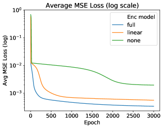
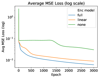
Figure 2: Average MSE error (log scale) during training phase. Left: 1394_sop_eir, right: 3375wp_mp.

VII-C Training Convergence and Speed

The key motivation of this paper is to speed up the learning task. This section demonstrates that the OPF-DNN architecture with load encoding quickly converges to an accuracy that is an order of magnitude better than full OPF-DNN architecture. Figure 2 shows the combined MSE losses (in log scale) for the three OPF-DNN architectures during the training phase for the 1394 and 3375 bus benchmarks. The results are averaged by the number of training cases as in previous sections. The full NN-encoder is almost an order of magnitude more accurate than the base model, and consistently better than the linear encoder model. Both load-encoding architectures outperforms the base model in the early convergence period (within 500 epochs), and a significant convergence gap still exists even after the error curves have flattened (e.g., after 2500 epochs). These results indicate that load reduction yields both a better training convergence and smaller prediction errors.

VIII Conclusion

This paper studied how to improve the scalability of deep neural networks for learning the active and reactive power of generators in AC-OPF. To address computational issues that arise in learning AC-OPF over large networks, this paper proposed a load encoding scheme for dimensionality reduction and its associated deep learning architecture. The load encoding scheme consists of (1) an optimization model to aggregate loads for each instance; and (2) a deep learning model that approximates the load encoding. The learned encoder can then be included in a deep learning architecture for AC-OPF and produces an order of magnitude improvement in training convergence and prediction accuracy of large realistic cases.

References

- [1] B. H. Chowdhury, S. Rahman, A review of recent advances in economic dispatch, IEEE Transactions on Power Systems 5 (4) (1990) 1248–1259.
- [2] F. Fioretto, T. W. Mak, P. Van Hentenryck, Predicting ac optimal power flows: Combining deep learning and lagrangian dual methods, in: Proceedings of the AAAI Conference on Artificial Intelligence, 2020, pp. 630–637.
- [3] Z. Yan, Y. Xu, Real-time optimal power flow: A lagrangian based deep reinforcement learning approach, IEEE Transactions on Power Systems 35 (4) (2020) 3270–3273.
- [4] X. Pan, T. Zhao, M. Chen, Deepopf: Deep neural network for dc optimal power flow, in: 2019 IEEE International Conference on Communications, Control, and Computing Technologies for Smart Grids (SmartGridComm), 2019, pp. 1–6.
-
[5]
P. V. Hentenryck,
Machine
Learning for Optimal Power Flows, Ch. 3, pp. 62–82.
doi:10.1287/educ.2021.0234.
URL https://pubsonline.informs.org/doi/abs/10.1287/educ.2021.0234 - [6] M. Chatzos, T. Mak, , P. Van Hentenryck, Spatial network decomposition for fast and scalable ac-opf learning, IEEE Transactions on Power Systems (2021) to appear.
-
[7]
C. Coffrin, D. Gordon, P. Scott, NESTA,
the NICTA energy system test case archive, CoRR abs/1411.0359.
URL http://arxiv.org/abs/1411.0359 - [8] S. Babaeinejadsarookolaee, A. Birchfield, R. D. Christie, C. Coffrin, C. DeMarco, R. Diao, M. Ferris, S. Fliscounakis, S. Greene, R. Huang, C. Josz, R. Korab, B. Lesieutre, J. Maeght, T. W. K. Mak, D. K. Molzahn, T. J. Overbye, P. Panciatici, B. Park, J. Snodgrass, A. Tbaileh, P. V. Hentenryck, R. Zimmerman, The power grid library for benchmarking ac optimal power flow algorithms, arXiv 1908.02788.
- [9] J. B. Ward, Equivalent circuits for power-flow studies, Transactions of the American Institute of Electrical Engineers 68 (1) (1949) 373–382.
- [10] H. K. Amchin, E. T. B. Gross, Analyses of subsequent faults, Electrical Engineering 71 (5) (1952) 420–420.
- [11] W. Jang, S. Mohapatra, T. J. Overbye, H. Zhu, Line limit preserving power system equivalent, in: 2013 IEEE Power and Energy Conference at Illinois (PECI), 2013, pp. 206–212.
- [12] S. Y. Caliskan, P. Tabuada, Kron reduction of power networks with lossy and dynamic transmission lines, in: 2012 IEEE 51st IEEE Conference on Decision and Control (CDC), 2012, pp. 5554–5559.
- [13] I. P. Nikolakakos, H. H. Zeineldin, M. S. El-Moursi, J. L. Kirtley, Reduced-order model for inter-inverter oscillations in islanded droop-controlled microgrids, IEEE Transactions on Smart Grid 9 (5) (2018) 4953–4963.
- [14] Z. Jiang, N. Tong, Y. Liu, Y. Xue, A. G. Tarditi, Enhanced dynamic equivalent identification method of large-scale power systems using multiple events, Electric Power Systems Research 189 (2020) 106569.
- [15] S. Tasnim, A. Rahman, A. M. T. Oo, M. E. Haque, Autoencoder for wind power prediction, Renewables: Wind, Water, and Solar 4 (1) (2017) 6.
- [16] A. Gensler, J. Henze, B. Sick, N. Raabe, Deep learning for solar power forecasting — an approach using autoencoder and lstm neural networks, in: 2016 IEEE International Conference on Systems, Man, and Cybernetics (SMC), 2016, pp. 2858–2865.
- [17] A. Kundu, A. Sahu, E. Serpedin, K. Davis, A3d: Attention-based auto-encoder anomaly detector for false data injection attacks, Electric Power Systems Research 189 (2020) 106795.
- [18] C. Coffrin, R. Bent, K. Sundar, Y. Ng, M. Lubin, Powermodels. jl: An open-source framework for exploring power flow formulations, in: 2018 Power Systems Computation Conference (PSCC), 2018, pp. 1–8.
- [19] A. Paszke, S. Gross, S. Chintala, G. Chanan, E. Yang, Z. DeVito, Z. Lin, A. Desmaison, L. Antiga, A. Lerer, Automatic differentiation in pytorch, NIPS 2017 Workshop (2017).