Simulating Yang-Mills theories with a complex coupling

Abstract

We propose a novel simulation strategy for Yang-Mills theories with a complex coupling, based on the Lefschetz thimble decomposition. We envisage, that the approach developed in the present work, can also be adapted to QCD at finite density, and real time simulations.

Simulations with Lefschetz thimbles offer a potential solution to sign problems in Monte Carlo calculations within many different models with complex actions. We discuss the structure of Generalized Lefschetz thimbles for pure Yang-Mills theories with a complex gauge coupling $\beta$ and show how to incorporate the gauge orbits. We propose to simulate such theories on the union of the tangential manifolds to the relevant Lefschetz thimbles attached to the critical manifolds of the Yang-Mills action. We demonstrate our algorithm on a (1+1)-dimensional U(1) model and discuss how, starting from the main thimble result, successive subleading thimbles can be taken into account via a reweighting approach. While we face a residual sign problem, our novel approach performs exponentially better than the standard reweighting approach.

I Introduction

The notorious sign problem hampers numerical simulations of many interesting physical systems, ranging from high energy to condensed matter systems. A sign problem is faced in numerical calculations of statistical models whenever the action becomes genuinely complex. Hence, standard Monte Carlo methods and in particular importance sampling drastically lose their efficiency with increasing lattice volume.

Examples of theories with a sign problem include real time calculations in lattice-regularized quantum field theories, i.e. lattice QCD in Minkowski space-time, lattice QCD with a nonzero vacuum angle $\theta$, and lattice QCD with a nonzero baryon chemical potential $\mu_{B}$. For the latter two cases, many methods have been developed that potentially circumvent or solve this problem in the continuum limit. These methods include reweighting Barbour et al. (1998); Fodor and Katz (2002), Taylor expansions Allton et al. (2002, 2003); Gavai and Gupta (2003), analytic continuation from purely imaginary chemical potentials de Forcrand and Philipsen (2002); D’Elia and Lombardo (2003), canonical partition functions Kratochvila and de Forcrand (2004); Alexandru et al. (2005), strong coupling/dual methods Karsch and Mutter (1989); de Forcrand et al. (2014); Gattringer and Langfeld (2016); Gagliardi and Unger (2020), the density of states method Ambjorn et al. (2002); Fodor et al. (2007); Langfeld et al. (2016), and complex Langevin dynamics Karsch and Wyld (1985); Aarts et al. (2010, 2013); Sexty (2014), see Attanasio et al. (2020) for a review of recent developments. However, all these methods so far face severe limitations that restrict their applicability in the continuum limit.

In the past decade deformations of the original integration manifold into the complex domain have been introduced, based on complex saddle points of the action, the Lefschetz thimbles Pham (1983); Witten (2010). If these deformations are chosen well, all physical expectation values obtained from an oscillatory integral remain unchanged but the sign problem is drastically alleviated. Thus, a numerical evaluation of the theory is accessible. By definition, the imaginary part of the action (phase of the probability density) is stationary on the thimble. A first Lefschetz thimble algorithm in the context of the QCD finite density sign problem was introduced in Cristoforetti et al. (2012), for a recent review see Alexandru et al. (2020). Despite its great potential for beating the sign problem, simulations with Lefschetz thimbles have to overcome the following intricacies:

• A parametrization of the thimble is a priori unknown and has to be obtained as the numerical solution of a flow-equation. The parametrization and the necessary Jacobian of the variable transformation are numerically demanding.

• The curvature of the thimble manifold introduces a so-called residual sign problem through the Jacobian.

• In most cases, one has to include relevant contributions from a large number of thimbles. Their relative weight may give rise to a further, residual, sign problem. In any case, the probability density becomes multi-modal.

These shortcomings have been addressed by formulating particularly efficient methods for the calculation of the Jacobian Cristoforetti et al. (2014); Alexandru et al. (2017a), by optimizing the deformation of the integration domain either based on a model ansatz Bursa and Kroyter (2018); Mori et al. (2017) or by means of machine learning Mori et al. (2018); Alexandru et al. (2017b); Wynen et al. (2020) and finally by using tempering Alexandru et al. (2017c); Fukuma et al. (2019) and other advanced strategies to foster transitions between thimbles and take into account contributions from multiple thimbles Di Renzo and Eruzzi (2018); Bluecher et al. (2018); Di Renzo et al. (2020).

In the present work we analyze the structure of the Lefschetz thimble decomposition of pure gauge theories with gauge groups $\text{U}(N)$ and $\text{SU}(N)$ and complex coupling $\beta$. We propose to sample on the tangential manifold attached to the thimble of the main critical point, i.e. the critical point with the smallest action value. As expected, we find a full hierarchy of critical points (saddle points) that have to be considered depending on the coupling parameter $\beta$. We include successive subleading saddle point contributions via reweighting. The reweighting procedure is set up by using linear mappings from the main tangential manifold to the tangential manifold attached to the thimble of the target critical point.

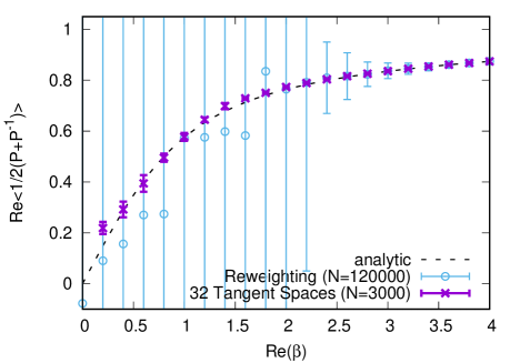
Figure 1: Comparison of the novel Takagi simulation method with standard reweighting on an $8\times 8$ lattice with gauge group $\mathrm{U}(1)$, where we measured the real part of the average plaquette. We vary the real part of $\beta$, while keeping $\mathrm{Im}\,(\beta)=1$ constant. Both reweighting and our approach took about the same amount of computing time.

Our approach has the following advantages over the flow-based generalized Lefschetz thimble approach Alexandru et al. (2016a):

• During the sampling procedure, we neither have to flow our configuration nor have to calculate a Jacobian since it is constant on the tangential manifold.

• As contributions from subleading thimbles are taken into account by reweighting Bluecher et al. (2018), there is no ergodicity problem due to potential barriers between thimbles. The reweighting procedure does also not introduce any overlap problem since critical points are mapped onto critical points.

The disadvantages are:

• Sampling on the tangential manifold rather than on the thimble itself does not completely resolve the sign problem, however, there is no residual sign problem from the Jacobian Cristoforetti et al. (2014).

• The critical points need to be known.

The advantages are clearly demonstrated for the benchmark case of an $\mathrm{U}(1)$ gauge theory, as summarized in Fig. 1. There we compare our results for the real part of the plaquette with that produced by the standard reweighting procedure. For the same numerical costs the error bars of our results are reduced by orders of magnitude.

This will be discussed in more detail in this work, which is organized as follows: In Sec. II we derive necessary formulas for our setup. Emphasis is devoted to discussing the critical manifolds of the Yang-Mills action as well as the Lefschetz thimbles. Moreover we explain our update and reweighting procedures. In Sec. III we apply our algorithm to the case of a 2-dimensional $\text{U}(1)$ gauge theory. In Sec. IV we discuss prospect of our approach. Finally we conclude in Sec. V.

II Formulation

II.1 Overview

We consider the standard discretization of the Yang-Mills action Wilson (1974)

$$S=\beta\sum_{x}\sum_{\mu<\nu}\left\{1-\frac{1}{2N}\left(\text{Tr}P_{\mu,\nu}(x)+\text{Tr}P^{-1}_{\mu,\nu}(x)\right)\right\}\,,$$ (1)

where $P_{\mu,\nu}(x)=U_{\mu}(x)U_{\nu}(x+\hat{\mu})U^{-1}_{\mu}(x+\hat{\nu})U^{-1}_{\nu}(x)$ denotes the elementary plaquette in the ($\mu,\nu$)-plane at lattice site $x\in\Lambda$ where $\Lambda\subset\mathbb{Z}^{d}$. The summation is done such that each plaquette is counted with only one orientation. The link variables $U_{\mu}(x)$ are elements of the gauge group, which we consider to be a Lie group and in particular $\text{U}(N)$ or $\text{SU}(N)$.

A sign problem is introduced by choosing general complex couplings $\beta$.

We aim to update a given gauge field configuration such that the imaginary part of the action $\text{Im}(S)$ varies slowly and hence the remaining sign problem is mild.

In order to achieve this goal the link variables are complexified, i.e. they are allowed to take values within the larger group $\text{GL}(N,\mathbb{C})$ or $\text{SL}(N,\mathbb{C})$, respectively. By generalized Picard-Lefschetz theory, there is a smooth middle dimensional manifold connected to each complex critical manifold (simply connected union of points, where $\nabla S=0$) of the action on which $\text{Im}(S)$ stays constant. These manifolds are called Lefschetz thimbles. As already stated, updates that stay on these thimbles are computational very demanding and are invariably global updates Cristoforetti et al. (2012, 2013); Fujii et al. (2013); Alexandru et al. (2016a). To reduce the computational demand, it has been argued that one does not have to stay exactly on the thimble in order to reduce the sign problem significantly Alexandru et al. (2016b); Mori et al. (2017). Any deformation of the original integration domain which has the correct asymptotic behavior will be sufficient. Here we construct an integral deformation, which is the union of all tangential manifolds to the critical points. As for the pure gauge theory all critical manifolds are known, this manifold is straightforward to parametrize. After discussing the critical manifolds in Sec. II.2 and II.3 we discuss properties of Lefschetz thimbles and tangential manifolds in Sec. II.4 and II.5. Our algorithmic approach is presented in Sec. II.6, II.8 and II.7.

II.2 The critical points of the Yang-Mills action

A Lefschetz thimble is generally defined to be the union of flow lines generated by the steepest descent equation

$$\frac{\mathrm{d}U}{\mathrm{d}t}=-\left(\frac{\delta S}{\delta U}\right)^{*}\,,$$ (2)

which end in a non-degenerate critical point of the action. The degeneracy of critical points due to gauge symmetry necessitates the application of Witten’s concept of generalized Lefschetz thimbles (Witten, 2011, 3.3).

The critical manifolds can be described in terms of plaquette variables. This is seen by examining the gradient of the action

$$\,\partial_{x,\kappa,a}S=-\frac{i\beta}{2N}\times$$ (3)

$$\,\mathrm{Tr}\left[\left(\sum_{\kappa<\nu}P_{\kappa,\nu}(x)-P^{-1}_{\kappa,\nu}(x)+P_{\kappa,-\nu}(x)-P^{-1}_{\kappa,-\nu}(x)\right.\right.$$

$$\,-\left.\left.\sum_{\mu<\kappa}P_{\mu,\kappa}(x)-P^{-1}_{\mu,\kappa}(x)+P_{-\mu,\kappa}(x)-P^{-1}_{-\mu,\kappa}(x)\right)t_{a}\right]\,.$$

Here $t_{a}$ are the generator matrices of the related Lie-Algebras $\mathfrak{su}(N),\mathfrak{u}(N)$. In our notation those are Hermitian, and for $N>1$ they satisfy the normalization condition $\mathrm{Tr}[t_{a}t_{b}]=\frac{1}{2}\delta_{ab}$. The derivative with respect to the gauge link $U$ in the direction of $t_{a}$ is defined as $\partial_{a}f(U):=\frac{\partial}{\partial\omega}f(e^{i\omega t_{a}}U)|_{\omega=0}$. Negative signs in the subscript of the plaquette variables refer to reversed directions in their orientation, e.g.

$$P_{\kappa,-\nu}(x)=U_{\kappa}(x)U_{\nu}^{-1}(x+\hat{\kappa}-\hat{\nu})U_{\kappa}^{-1}(x-\hat{\nu})U_{\nu}(x-\hat{\nu})\,.$$

A necessary condition for a critical configuration is a vanishing gradient of the action.

In the following we derive relations that constrain possible plaquette values from a critical configuration. Eq. (3) vanishes $\forall\ a$, if the matrix in round brackets is proportional to $\mathbbm{1}$ for plaquette values in $\text{SL}(N,\mathbb{C})$. For plaquette values in $\text{GL}(N,\mathbb{C})$, the matrix has to be zero. For a proof, see the App. D. This criticality condition yields relations for adjacent plaquettes sharing one link. Note that in $d$ dimension one link is shared by $2(d-1)$ plaquettes.

We exemplify the $d=2$ case: For plaquette values in $\text{GL}(N,\mathbb{C})$, we can directly read off the relations

$$P_{1,2}(x)=P^{-1}_{1,-2}(x)\>\>\text{or}\>\>P_{1,2}(x)=-P_{1,-2}(x)\,,$$

and

$$P_{1,2}(x)=P^{-1}_{-1,2}(x)\>\>\text{or}\>\>P_{1,2}(x)=-P_{-1,2}(x)\;.$$ (4)

If we assume that our critical configuration consists of commuting (Abelian) link variables, i.e. if link variables are diagonal, the above relation simplifies to

$$P_{1,2}(x)=P_{1,2}(x-\hat{\nu})\;\;\text{or}\;\;P_{1,2}(x)=-P^{-1}_{1,2}(x-\hat{\nu})\,,$$ (5)

with $\nu\in\{1,2\}$. It follows that each critical configuration exhibits at most two distinct plaquettes values. If plaquettes take values in $\text{SL}(N,\mathbb{C})$ we get, e.g., for a link in $\hat{1}$-direction

$$(P_{1,2}(x)-P^{-1}_{1,2}(x)-P^{-1}_{1,-2}(x)+P_{1,-2}(x))=\alpha\mathbbm{1}\,,$$ (6)

for an arbitrary $\alpha\in\mathbb{C}$. For the Abelian case, this equation reformulates again to a relation between adjacent plaquettes. Restricting this further to the original group $\mathrm{SU}(N)$, i.e. the maximal torus of $\mathrm{SU}(N)$, we find

$$(\mathrm{Im}\,P_{1,2}(x)-\mathrm{Im}\,P_{1,2}(x-\hat{\nu}))_{ii}=\\ (\mathrm{Im}\,P_{1,2}(x)-\mathrm{Im}\,P_{1,2}(x-\hat{\nu}))_{jj}\;\forall i,j,\nu\,.$$ (7)

For $d>2$, we obtain the same constraint on the imaginary parts of diagonal entries of adjacent plaquettes, but naturally there are more adjacent plaquettes.

From the periodic boundary condition we can derive further constraints. Under the assumption, that the relevant critical configurations are Abelian, the product of all plaquettes in an arbitrary 2-dimensional hyperplane $\Lambda_{\mu\nu}$ must be one, i.e.

$$\prod_{x\in\Lambda_{\mu\nu}}P_{\mu\nu}(x)=1\,.$$ (8)

II.3 Locality and critical manifolds

We are left with a fairly large number of critical configurations, which we will boil down to a set of basis configurations, getting the others by transpositions and symmetry relations. The ultimate aim is to obtain a homotopic covering of the original integration domain $[\mathrm{U}(N)]^{dV}$ or $[\mathrm{SU}(N)]^{dV}$ .

As a guiding inspiration, we start with a discussion of the one-plaquette model, i.e. we just have only one plaquette degree of freedom, as Eq. (1) is a sum of local plaquette terms. The action is defined as

$$S=-\frac{\beta}{2N}\mathrm{Tr}\left[P+P^{-1}\right]\,,$$ (9)

where an irrelevant constant has been omitted. The Lie derivatives with respect to $P$ are given by

$$\partial_{a}S=-\frac{i\beta}{2N}\mathrm{Tr}\left[(P-P^{-1})t_{a}\right]\,.$$ (10)

Observations are:

• Eq. (10) vanishes for self-inverse plaquettes $P$ in $\mathrm{U}(N)$. Therefore, the critical points consists only of matrices whose eigenvalues are $+1$ and $-1$.

• For $P\in\mathrm{SU}(N)$ Eq. (7) implies that the imaginary part of all eigenvalues must be identical. For vanishing imaginary part we obtain the self-inverse elements of $\mathrm{SU}(N)$. The constraint $\det[P]=1$ implies an even number of ($-1$)-eigenvalues, denoted by $N^{(-)}$. For non-vanishing imaginary part, the center elements of $\mathrm{SU}(N)$ are solutions. For $N\geq 6$, we have roots of unity apart from $\pm 1$ with the same imaginary parts. So a mixing of these yielding a unit determinant is a valid solution.

Different critical points indicate different action values. Their importance with respect to the weight factor $w\equiv e^{-\mathrm{Re}\,(S)}$ may be exponentially suppressed. For the one-plaquette model we find the following hierarchy of critical points: For $P\in\mathrm{U}(N)$, we have

$$S=-\frac{\beta}{N}\left(N-N^{(-)}\right)\,.$$ (11)

The importance of a critical point thus shrinks with the number of ($-1$)-eigenvalues. For $\mathrm{SU}(3)$, we find 6 critical points with three different action values

$$S=-\beta\,, \quad P=\mathbbm{1}$$

$$S=-\frac{\beta}{2}\,, \quad P\in\left\{e^{i\frac{2\pi}{3}k}\mathbbm{1}\,,\;k=1,2\right\}$$

$$S=-\frac{\beta}{3}, \quad P\in\left\{\text{diag}(1,-1,-1),\;\text{diag}(-1,1,-1),\right.$$

$$\left.\qquad\quad\text{diag}(-1,-1,1)\right\}\,.$$ (12)

Critical points from the one-plaquette model can be used to construct certain critical configurations for the full lattice theory. We pick critical plaquette values from the one-plaquette model and distribute them in accordance with Eq. (4) and (6) over the lattice. Each critical configuration obtained in this way is one representative of a critical manifold, which consists of its gauge orbit and additional zero modes of the action. For this simple procedure we obtain an additional constraint from Eq. (8): The product of eigenvalues at every position over every two-dimensional hyperplane must be one. We are therefore limited to configurations, where the number of ($-1$)-eigenvalues at a given diagonal entry is even (the $\mathrm{U}(N)$ case) in every hyperplane or in principal their overall product is one including additional roots of unity.

Note however, that not all critical configurations can be found by the above prescription. Recall that Eq. (4) restricts the plaquette values in a hyperplane at any given position to only two possible values. We can construct a further critical configuration by setting one (or more) plaquette values in that hyperplane to $e^{i\epsilon}$, while choosing $e^{i(\pi-\epsilon)}$ for all remaining plaquettes in the hyperplane. Possible $\epsilon$ values are constrained by Eq. (8), and hence

$$k\pi+(V-2k)\epsilon=2\pi l\,,$$ (13)

where $k$ is the number of plaquettes with the specific diagonal entry $e^{i(\pi-\epsilon)}$. The $2\pi l$ factor stems from the $2\pi$ periodicity. For $d=2$, $N=1$, $l$ is the actual topological charge. It is constant on the thimble, since the anti-holomorphic gradient flow can be seen as an analytic continuation of the classical gradient flow, which leaves the topological charge invariant Lüscher (2010). Note especially for $k\neq V/2$, that $\epsilon$ has to be a real number, so the critical configurations are all in the original group space. Picard-Lefschetz theory tells us now, that if the tangent space of the thimble is not normal at this point to the original group manifold, then the intersection number is non-zero (in our case one). We will see, that for $\mathrm{Im}\,\beta\neq 0$, this is the case and they all contribute. For $\mathrm{SU}(N)$, we have to add the constrain that the determinant equals one, effectively reducing the number of critical configurations.

II.4 The Takagi decomposition and generalized Lefschetz thimbles

Next, we construct the tangent spaces at each critical manifold described Sec. II.3. To that end we solve the Takagi equation

$$H^{*}\xi^{*}=\lambda\xi\>\>\text{with}\>\>\lambda\in\mathbb{R}\,.$$ (14)

Here $H$ denotes the Hessian of the action evaluated on the critical manifold. Modes $\xi$ associated with positive $\lambda$, point in the direction of the thimble. In the following we refer to such a mode as Takagi vector. Correspondingly, a mode $\xi$ associated with a negative $\lambda$ points in direction of the anti-thimble. It is called anti-Takagi vector (see e.g. Alexandru et al. (2016a)) The $\lambda=0$ vectors do not change the action and are therefore referred to as zero-modes. They result for instance from the gauge degrees of freedom. The Hessian of the action can be written as

$$\partial_{x,\kappa,a}\partial_{y,\eta,b}S = \frac{\beta}{2N_{c}}\mathrm{Tr}\left[\left(\sum_{U_{\kappa}(x),U_{\eta}(y)\in P}(P+P^{-1})\right.\right.$$

$$+ \sum_{U^{-1}_{\kappa}(x),U^{-1}_{\eta}(y)\in P}(P+P^{-1})$$

$$- \sum_{U_{\kappa}(x),U^{-1}_{\eta}(y)\in P}(P+P^{-1})$$

$$- \left.\left.\sum_{U^{-1}_{\kappa}(x),U_{\eta}(y)\in P}(P+P^{-1})\right)t_{b}t_{a}\right]\,,$$ (15)

where the plaquettes appear in different orientations depending on the position of the referred link. Since by construction we have considered only those representatives of our critical manifolds which have diagonal links. They are Abelian and we can permute our variables to bring all generators to the right.

For critical configurations, where the plaquettes are elements of the original group, the Hessian splits into a real matrix with a complex prefactor $H=\beta M$, whose eigenvectors $v$ and eigenvalues $\alpha$ can be computed. For $\alpha\neq 0$, the solutions to Eq. (14) take the form

$$\xi^{(\pm)}=\sqrt{\frac{\pm\mathrm{sign}(\alpha)\beta^{*}}{|\beta|}}\;v\,,$$ (16)

where the $\xi^{(+)}$ ($\xi^{(-)}$) indicate the thimble (anti-thimble) directions. The $\alpha=0$ eigenvectors correspond to the $\lambda=0$ solutions of Eq. (14) and can have an arbitrary complex prefactor.

We observe that for most of our critical configurations. We will come to the exceptions in Sec. III.2. The Hessian does not change under field transformations in the direction of these zero modes. Consequently the critical manifold $\{U^{\mathrm{crit},0}_{\mu}(x)\}$ is independent of those. Therefore, we can deduce that the projection of the subspace spanned by its zero modes in the Lie algebra is the critical manifold itself.

$$\left\{U^{\mathrm{crit}}_{\mu}(x)=U^{\mathrm{crit},0}_{\mu}(x)\exp\left[{i\sum_{k,a}\tilde{b}_{k}v^{x,\mu,a}_{k}(\alpha=0)t_{a}}\right]\right.\\[8.61108pt] \left|\vphantom{\sum_{k,a}}\tilde{b}_{k}\in\mathbb{C},\;x\in\Lambda,\;\mu=1,\ldots,d\right\}\,.$$ (17)

The $k$ index enumerates the different zero-eigenvectors $v$ of matrix $M$. For $\tilde{b}_{k}\in\mathbb{R}$, this is a compact manifold. In complexified space with $\tilde{b}_{k}\in\mathbb{C}$, we have non-compact imaginary directions. Nevertheless, the manifold is still critical. To obtain the generalized Lefschetz thimble Witten (2011), we start with a compact submanifold (a cycle) of real dimension $\#(\alpha=0)=n^{(0)}$. Therefrom its tangent space is spanned. The compact submanifold is commonly called gauge orbit. At every point of this cycle, we use the $\alpha\neq 0$ Takagi vectors to span the rest of the tangent space. Since the latter is invariant under zero-modes a point on this tangent space can be directly written in terms of

$$U_{\mu}(x)=U^{\mathrm{crit},0}_{\mu}(x)\exp\left[{i\sum_{k,a}b_{k}c_{k}v^{x,\mu,a}_{k}t_{a}}\right],\\ \text{with}\;\;b_{k}\in\mathbb{R}\;\text{and}\;\;c_{k}=\begin{cases}1&,\;\alpha_{k}=0\\ \sqrt{\frac{\mathrm{sign}(\alpha_{k})\beta^{*}}{|\beta|}}&,\;\alpha_{k}\neq 0\,.\end{cases}$$ (18)

Here the summation index $k$ runs over all eigenvectors. The real dimension $n$ of the thimble thus splits into zero and non-zero mode directions as $n=n^{(0)}+n^{(+)}=dVN_{g}$, where $N_{g}$ is the dimension of the Lie algebra. This construction can be generalized to more complicated Hessians, see App. A.

If we do not conform to that construction, e.g., tilt the real vectors by a complex factor, we loose homotopy to the generalized Lefschetz thimble. The resulting manifold is non-compact, see Fig. 2.

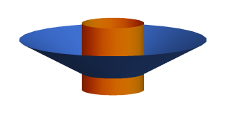
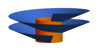
Figure 2: Upper plot: Schematic picture of the generalized Lefschetz thimble, spanned on a compact submanifold as proposed by Witten (Witten, 2011, 3.3). Lower plot: The thimble will exhibit infinitely many Riemann surfaces if we choose a noncompact submanifold from the critical cylinder. In both plots the critical cylinder is depicted in orange and the thimble in blue.

However, the non-compact directions refer to zero-modes, i.e. they leave the action invariant. This corresponds to multiplying the partition sum with an infinite volume factor, which drops out for all physical observables, when calculating expectation values. The prerequisite for these observables is, that they are independent from the zero-modes, i.e. that they are gauge-invariant observables.

The global minimum among our critical manifolds is given by $\{P_{\mu\nu}(x)=\mathbbm{1}\;\forall\;x,\mu<\nu\}$. Since this is a minimum in the non-complexified gauge theory, the matrix $M$ is positive semidefinite. As the gauge field is constant, the complex prefactor is identical to all Takagi-modes. We are free to choose the same complex prefactor also for the real zero-modes. Since the eigenvectors of $M$ span the whole $\mathbb{R}^{n}$ space and since we chose the same complex prefactor for all directions, we can make a basis transformation to the unit basis $\{e_{1},\ldots,e_{n}\}$. Moving in one of these directions $e_{i}$ corresponds to a change of a single (local) color degree of freedom. This basis can thus be used to construct a local update algorithm on the generalized main Lefschetz thimble, see Sec. II.8.

As we are interested in a single homotopic covering of our original compact integration domain, we need to limit the tangent spaces.

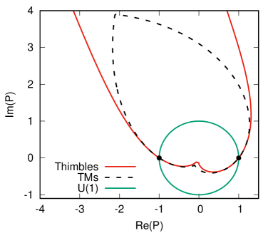
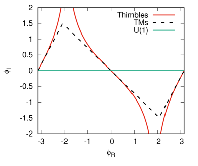
Figure 3: Lefschetz thimbles and tangential manifolds (TMs) bounded by their intersection for the one-plaquette model at $\beta=1+3i$ in group and angular (algebra) representation.

It turns out that the construction of a continous manifold that is homotopic to the original integration domain is the main conceptual difficulty in this approach. For the $\mathrm{U}(1)$ one-plaquette model, we have only two critical points and tangent spaces. They give, when glued together at their intersections, a manifold homotopic to $\mathrm{U}(1)$, see Fig. 3. We introduce boundaries on the main tangential manifold by identifying intersections with the tangential spaces of the other subleading critical manifolds. We will call these limited tangent spaces, tangential manifolds (TM) from now on. For the full lattice theory we discuss several possible choices of boundaries throughout this work.

II.5 Hierarchy of critical manifolds

The choice of critical manifolds introduces a natural hierarchy which is reflected by the values of the action. Their importance decreases according to their weight factor $e^{-S}$ with increasing action. Given our choice of critical configurations with diagonal plaquettes from the original integration domain ($\mathrm{U}(N)$ or $\mathrm{SU}(N)$), we can easily express the action in terms of the plaquette eigenvalues. We find

$$S=\beta\sum_{x}\sum_{\mu<\nu}\left[1-\frac{1}{N}\sum_{k=1}^{N}\cos(\phi_{\mu,\nu}^{(k)}(x))\right]\,,$$ (19)

where the $\phi_{x}^{(k)}$ is the angle of the $k$-th eigenvalue of the plaquette $P_{\mu\nu}(x)$. These critical action values are minima of the attached thimbles, since the real part of the action naturally increases if one moves away from the critical manifolds for $\mathrm{Re}\,(\beta)>0$ in Takagi direction. This is still true, if one considers the Thimble tangent space in a region around the critical manifold, limiting it to a TM. The main critical point ($\phi_{x}^{(k)}=0\;\forall x,k$) defines the global minimum of the action in this many TMs scenario. Consequently with increasing $\mathrm{Re}\,(\beta)$, certain TMs become exponentially suppressed and we obtain a pronounced hierarchy with the main TM as leading order. For purely imaginary values of $\beta$, every thimble contributes equally.

II.6 Update algorithm on a TM with a Takagi basis

Next, we discuss possible sampling algorithms that are restricted to a single TM. Following our strategy to span the tangent space by the Takagi vectors and real zero-modes, we readily have a parametrization at hand. According to Eq. (18) we can express each configuration on the tangent space by real coordinates $b_{k}$, specifying a vector in the Lie-algebra. Note that for the zero-modes ($\alpha=0$) we have no complex prefactor. Using these coordinates, one can think of applying various different update procedures on the tangent space, starting from a single random walk Monte Carlo (crude Monte Carlo), over a Hybrid Monte Carlo to a trained flow-based neural network Kanwar et al. (2020); Boyda et al. (2020). The important steps are:

1. Choose a critical configuration, to specify the tangent space on which to carry out the updates. This configuration may also serve as starting configuration.

2. Calculate the real Hessian $M$ and determine its eigenpairs ($\alpha_{i}$, $v_{i}$). This has to be done only once for a given critical configuration, independent of the coupling $\beta$.

3. Propose a new configuration by drawing a set of real coordinates $b_{k}$. The proposed configuration is than specified according to Eq. (18). Perform an accept/reject step based on the real part of the action difference between the old and new configuration. If the proposed configuration is outside the boundaries of the TM, we assign to it a zero probability and reject the proposed configuration, recording the old configuration like in the Metropolis algorithm.

4. Finally take the remaining sign problem into account by reweighting with the imaginary part of the action.

II.7 Leading and subleading thimbles

So far, we have restricted the sampling to a single TM attached to a specific critical configuration. Ultimately, we are interested in sampling a compact manifold that is homotopic to the original integration domain. In the standard thimble decomposition the combination of various Lefschetz thimble leads, by definition, to a multi-modal probability distribution. Sampling such distributions by a Monte Carlo procedure is difficult. As a solution, a tempered sampling procedure was proposed Alexandru et al. (2017c); Fukuma et al. (2019). Another possibility are independent Monte Carlo processes on each thimble. However, in this case the relative weights between thimbles need to be known. One possibility to infer these values is by using prior knowledge of a physical observable for normalization Di Renzo and Eruzzi (2018).

Here we construct a homotopic manifold by piecewise definition, where we use the TMs as building blocks. As our construction deviates from the thimble decomposition especially close to the boundaries, we do not have infinite action barriers between the patches. Hence, a sampling procedure that proposes configurations across boundaries would be in principle possible. However, we found that it is most convenient to sample the main tangent space with a single Monte Carlo chain and take all remaining patches into account via reweighting. We exemplify this procedure for a system of two TMs, $\tau_{0}$, $\tau_{1}$. Calculating expectation values over this extended region requires the relative weight $Z_{1}/Z_{0}$. Here $Z_{1}$ denotes the partition function corresponding to the subleading tangential manifold and $Z_{0}$ refers to the corresponding quantity on the main tangential manifold. It holds

$$\left<\mathcal{O}\right>_{\tau_{0}\cup\tau_{1}} =\frac{\int_{\tau_{0}}\mathrm{d}U~{}\mathcal{O}[U]e^{-S[U]}+\int_{\tau_{1}}\mathrm{d}U~{}\mathcal{O}[U]e^{-S[U]}}{\int_{\tau_{0}}\mathrm{d}U~{}e^{-S[U]}+\int_{\tau_{1}}\mathrm{d}U~{}e^{-S[U]}}$$

$$=\frac{\left<\mathcal{O}\right>_{\tau_{0}}+(Z_{1}/Z_{0})\left<\mathcal{O}\right>_{\tau_{1}}}{1+(Z_{1}/Z_{0})}\,.$$ (20)

Following the method proposed in Bluecher et al. (2018), we introduce a mapping

$$f\colon\tau_{0}\longrightarrow\;\;\tau_{1}\,.$$ (21)

It maps configurations from one of the two patches to the other. With this mapping we can express the ratio $Z_{1}/Z_{0}$ as

$$\frac{Z_{1}}{Z_{0}} =\frac{\int_{\tau_{0}}\mathrm{d}Ue^{-S[f(U)]+S[U]}\det[\mathrm{d}f]e^{-S[U]}}{\int_{\tau_{0}}\mathrm{d}Ue^{-S[U]}}$$

$$=\left<e^{-S\circ f+S}\det[\mathrm{d}f]\right>_{\tau_{0}}\,.$$ (22)

It remains to find a suitable $f$. Since we consider only tangent spaces, $f$ is linear and can be constructed as a basis transformation from the Takagi basis of $\tau_{0}$ to $\tau_{1}$. The Jacobian $\det[\mathrm{d}f]$ is therefore a constant factor. As the eigenbases of the real Hessian $M$ are orthogonal and can be chosen to have determinant one, the Jacobian depends consequently only on the the different sets of complex prefactors $c_{k}$ of the Takagi vectors. These depend in turn only on the sign of the eigenvalues $\alpha_{k}$. Therefore we find for the Jacobian

$$\det[\mathrm{d}f]=\frac{\left(\sqrt{\frac{-\beta^{*}}{|\beta|}}\right)^{n_{\tau_{1}}^{(-)}}}{\left(\sqrt{\frac{+\beta^{*}}{|\beta|}}\right)^{n_{\tau_{0}}^{(+)}-n_{\tau_{1}}^{(+)}}}\,,$$ (23)

where $n^{(+)}$ and $n^{(-)}$ are the number of positive/negative eigenvalues of the real Hessian $M$ (see Sec. II.4) at the respective patch. Here we assumed that $\tau_{0}$ is the patch attached to the main critical manifold having only positive eigenvalues being the global minimum. If the patches $\tau_{0}$ and $\tau_{1}$ are of different size, one may introduce an independent scale parameter to the mapping $f$, which is than also reflected as factor in the Jacobian. As the main tangential manifold is usually the largest such a factor is not necessarily needed in practice. It may however be used for optimization purposes.

II.8 Alternative updates on the main tangent space

As outlined in Sec. II.4 we can sample the main tangent space by just setting each complex factor $c_{k}$ to $\sqrt{{\beta^{*}}/{|\beta|}}$. In practice this tilts every link, since in this case all eigenvalues are positive or zero. Having identical complex prefactors, we can perform a basis transformation of our coordinates to the unit basis. Therein each coordinate corresponds to a single gauge degree of freedom. This allows for applying a local heat bath or Metropolis algorithm. The situation discussed here is shown at the bottom of Fig. 2. The unbounded critical manifold in imaginary direction has to be dealt with.

We limit the plaquette values in accordance with the intersection points of the tangent spaces in the one plaquette-model, creating TMs (see Fig. 3). Similarly as before, we define the region outside the boundary to have zero probability.

But since link variables can still diverge in imaginary direction we have to apply a second limit or just record variables, which are unaffected by the zero modes. In our theory, these are the plaquettes variables. An alternative is to adopt gauge cooling Seiler et al. (2013) to make this problem milder. A severe limitation of this method stems from the fact that only observables invariant under all zero-modes can be measured. Taking pure Yang-Mills theory it is not possible to measure the Polyakov loop. It is invariant under gauge transformations but not under a global zero mode. The latter is represented by changing all links in the same direction and amount leaving the plaquettes and therefore the action invariant.

III Application to a 2-dimensional $\text{U}(1)$-gauge theory

In this section we apply the above outlined method to two-dimensional pure $\mathrm{U}(1)$ gauge theory with periodic boundary conditions. Recently, complementary studies on this theory with a sign problem have appeared in the literature. In Hirasawa et al. (2020) the complex Langevin method is employed. The complex action here is caused by a non-zero vacuum angle. On the other hand in Kashiwa and Mori (2020) the theory with a complex gauge coupling is investigated by means of the path-optimization method.

III.1 The effective degrees of freedom

We formulate the theory in terms of its effective degrees of freedom.
Eq. (8) can be verified easily by noting that every link appears twice in all plaquettes. Hence the links cancel each other when being multiplied altogether. Consequently, one plaquette can be expressed in terms of all others. The action of the two-dimendional theory is rewritten as follows

$$S = -\frac{\beta}{2}\left[\sum_{(x,t)\neq(0,0)}\left(P_{1,2}(x,t)+P_{1,2}^{-1}(x,t)\right)\right.$$ (24)

$$+ \left.\left(\prod_{(x,t)\neq(0,0)}P_{1,2}^{-1}(x,t)+\prod_{(x,t)\neq(0,0)}P_{1,2}(x,t)\right)\right]\,,$$

neglecting constant terms. The last term is called toron term. One can reformulate the full theory in terms of these plaquettes variables having a reduced partition sum, which gives the same expectation values for observables that are invariant under zero modes

$$Z\;=\;\int\prod_{(x,t)\neq(0,0)}\mathrm{d}\theta(x,t)$$

$$\;\times\;\exp\left[\beta/2\sum_{(x,t)\neq(0,0)}\left(e^{i\theta(x,t)}+e^{-i\theta(x,t)}\right)\right]$$ (25)

$$\;\times\;\exp\left[\beta/2\left(e^{-i\sum_{(x,t)\neq(0,0)}\theta(x,t)}+e^{i\sum_{(x,t)\neq(0,0)}\theta(x,t)}\right)\right]\,.$$

For a full derivation see App. B. The periodic boundary conditions are represented by the toron term we placed at position $(0,0)$. Replacing this term by an independent plaquette term is equivalent to employing open boundary conditions. This shall be used as an approximation to the theory in the following. With open boundary conditions the integral factorizes in plaquettes variables yielding

$$Z=\left[\int_{\mathrm{U}(1)}\mathrm{d}Pe^{\beta/2(P+P^{-1})}\right]^{V}=\left[I_{0}(\beta)\right]^{V}\,.$$ (26)

The plaquette expectation value is then

$$<\frac{1}{2}(P+P^{-1})>=\frac{I_{1}(\beta)}{I_{0}(\beta)}\,,$$ (27)

which is exactly the the same as for the one-plaquette model. There is no volume dependence. Since the difference between periodic and open boundary conditions vanishes in the infinite volume limit, this is the expected value.
We construct the approximation scheme by successively including TMs as integration domains. Thereto we split the integral according to the critical points $P=\pm 1$ of the one plaquette model and get

$$Z = \left[\int_{\tau_{0}}\mathrm{d}Pe^{\beta/2(P+P^{-1})}+\int_{\tau_{1}}\mathrm{d}Pe^{\beta/2(P+P^{-1})}\right]^{V}$$ (28)

$$=: \left[Z_{0}+Z_{1}\right]^{V}=\sum_{k=0}^{V}\begin{pmatrix}V\\ k\end{pmatrix}Z_{0}^{V-k}Z_{1}^{k}\,.$$

We can map this to the lattice by $k$ denoting the number of plaquettes being $-1$ at the critical configuration. $\begin{pmatrix}V\\ k\end{pmatrix}$ is the number of such combinations on the lattice. Eq. (28) allows to calculate approximate values for the comparison with numerical simulations (see Fig. 4).

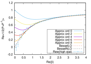
Figure 4: Thimble hierarchy depending on $\mathrm{Re}\,(\beta)$ in the approximation on a $4\times 4$ lattice at constant $\mathrm{Im}\,(\beta)=1$.

Complementary, there exists a formal solution for the for the full lattice theory with periodic boundary conditions involving no approximations. We can write the partition sum as

$$Z=\int\mathrm{d}U\exp\left({-S[U]}\right)=\sum_{n=-\infty}^{+\infty}\left[I_{n}(\beta)\right]^{V}\,,$$ (29)

being a series in modified Bessel functions $I_{n}(\beta)$, where $V$ is the number of plaquettes Balian et al. (1974); Migdal (1975). The leading order of this series corresponds to our approximation. The following orders take finite volume effects into account and yield the exact result provided that the series converges for the given value of $\beta$.

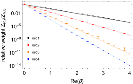
Figure 5: Comparison of the ratio of the partition functions $Z_{R,j}/Z_{R,0}=\langle\exp(-(S_{R,j}-S_{R,0}))\rangle_{0}$ i.e. the relative weights between the lowest four subleading and the leading order TMs (basis configurations). The index $j$ labels the subleading orders and the subscript $0$ indicates that the expectation value is calculated on the configurations measured on the leading order tangential surface, as in Bluecher et al. (2018). Here, the lattice is of size $4\times 4$, $\mathrm{Im}\,(\beta)=1$ and spherical boundaries are used. The data reflects very well the hierarchy described in Sec. III.2. As a comparison the functions $\exp(-S_{R}[P^{\mathrm{crit}}])$ are added to the plot in light colors.

III.2 Critical manifolds and their hierarchy

For an even number $k$ in Eq. (28) the critical configurations in the approximation and in the original lattice theory coincide. In contrast, for odd $k$, this does not hold due to the periodic boundary conditions. However, it is possible to construct critical manifolds being (arbitrarily) close to the corresponding configurations in the approximation. For odd $k<V/2-1$ we set $k$ plaquettes to $e^{i(\pi-\epsilon)}$ and the rest to $e^{i\epsilon}$ such that Eq. (13) is satisfied. This leads to the choice

$$\epsilon=\frac{\pi}{V-2k},$$ (30)

which we refer to together with the critical configurations for even $k$ as basis configurations from now on. Furthermore as discussed in Sec. II.3, Eq. (13) gives rise to a multiplet of configurations being related to the basis configurations by a symmetry. To see this, note that these $\epsilon$ configuration have topological charge $\lceil\frac{k}{2}\rceil$. Now, we can change the topological sector by adding/ subtracting $\frac{2\pi}{V-2k}$ from $\epsilon$. We observe that if $|\epsilon|<\pi/2$, the Takagi vectors do not change. Consequently we can apply this transformation directly to measured plaquettes values by multiplying them with $e^{\pm 2\pi/(V-2k)}$, where the sign is chosen whether we have a $e^{i(\pi-\epsilon)}$ or $e^{i\epsilon}$ plaquettes. This transformation does not only apply to odd $k$ but also to even $k$. By this procedure, we reach $2(V/4-\lceil\frac{k}{2}\rceil)$ critical manifolds in different topological sectors for odd $k$ and $2(V/4-1-\frac{k}{2})+1$ for even $k$, respectively.
Second, we can go from the $k$-th TM to the ($V\!\!-k$)-th TM by changing the plaquettes from the critical configuration according to

$$P^{\mathrm{crit}}_{1,2}(x)\;\longrightarrow\;-(P^{\mathrm{crit}}_{1,2}(x))^{-1}\,.$$ (31)

The corresponding real Hessian $M\rightarrow(-M)$ changes sign and has the same eigenvectors and zero modes. Only the non-zero eigenvalues $\alpha\rightarrow(-\alpha)$ change sign. Consequently and using the fact that eigenvectors are unique up to a non-zero scalar multiplication we get the Takagi vectors for the $(V\!\!-k)$-th TM by multiplying the Takagi vectors from the $k$-th TM by $\sqrt{-1}=i$. For $k\neq V/2,V/2\pm 1$, all zero modes do not change the plaquettes. Writing a plaquette configuration on the $k$-th tangent space as $P^{\mathrm{crit}}_{1,2}(x)e^{i\Delta\varphi(x)}$, we can write the mapping to the configuration on the opposite $(V\!\!-k)$-th tangent space as

$$P^{\mathrm{crit}}_{1,2}(x)e^{i\Delta\varphi(x)}\;\rightarrow\;-(P^{\mathrm{crit}}_{1,2}(x))^{-1}e^{-\Delta\varphi(x)}\,,$$ (32)

having again a transformation for directly measuring the plaquette values. Having these, the same procedure to reach the different topological sectors can be applied to these plaquette values.

An exception is the case $k=V/2$, which has an additional zero mode, which can be parametrized by

$$P_{12}(x)=e^{i\varphi}\;\text{and}\;P_{12}(x)=e^{i(\pi-\varphi)}\,,$$ (33)

for $V/2$ plaquettes on either side. This transformation necessarily leaves the action invariant while changing actual plaquettes values. The configurations, where all plaquettes are $\pm i$, which would be assigned to $k=V/2\pm 1$ in our scheme are included in this critical manifold and are therefore being left out. This transformation reduces the combinatorial factor to $\frac{1}{2}\begin{pmatrix}V\\ V/2\end{pmatrix}$.

The critical manifolds form a hierarchy depending on their associated value of the action

$$S\ \begin{cases}=2k\beta,&\>k\;\text{even},\\[4.30554pt] \approx\beta\left(2k+\frac{\pi^{2}}{2(V-2k)^{2}}\right),&\;k\;\text{odd}\,.\end{cases}$$

for the basis configurations. Depending on $\mathrm{Re}\,(\beta)$ the critical manifolds differ in importance for the partition sum since on thimbles and suitably bounded TMs the real part of the action is minimal at the critical manifold. Consequently, if $\beta$ is purely imaginary, every thimble or TM contributes equally. Otherwise one can obtain an approximate result by taking only a few thimbles or TMs into account as the others are exponentially suppressed. Fig. 5 illustrates the hierarchy of the critical manifolds considering subleading TMs up to order $k=4$ restricted to the basis configurations. The simulation setup used for the shown data is described in detail in Sec. III.4 and III.6.

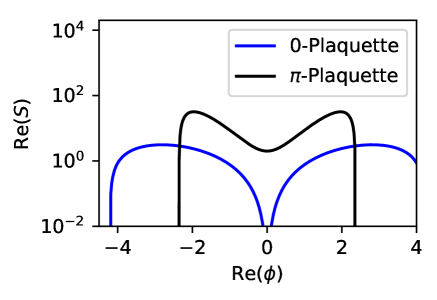
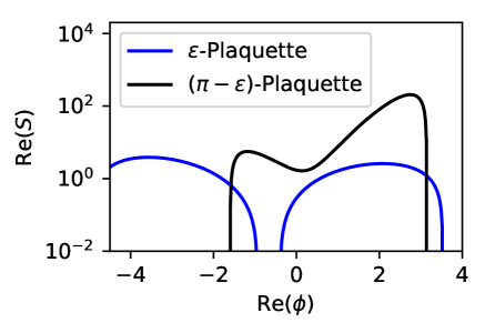
Figure 6: Real part of the action of a single plaquette on the tangent space of the thimble. At the top, we look at the situation $\phi=0$, i.e. $P=1$ and $P=-1$ like in the one plaquette model. In the plot below, we applied a shift $\epsilon=\pi/4$ to see the behaviour of shifted plaquettes, which we encounter in critical configurations with non-zero topological charge.

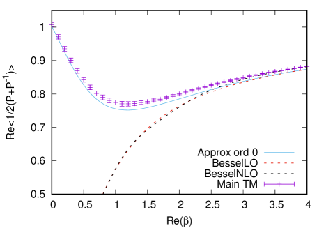
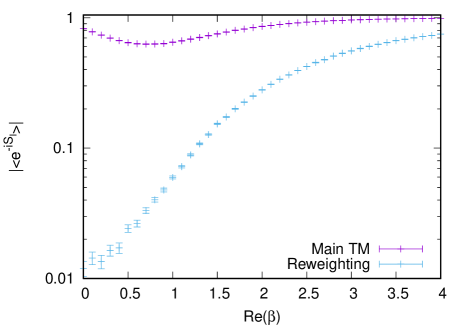
Figure 7: Result of the simulation on the main TM with real plaquette boundaries for constant $\mathrm{Im}\,(\beta)=1$ on a $4\times 4$ lattice. Note the fact that for high $\mathrm{Re}\,(\beta)$, the result approximates the BesselNLO result. This indicates that we simulate the actual lattice theory and not by accident a cartesian product of the one-plaquette model. On the right is the average sign compared with standard reweighting.

III.3 Ensuring homotopy

To ensure global homotopy, we need to make sure, that the TMs form a patchwork covering $\left[\mathrm{U}(1)\right]^{2V}$. Therefore, we have to create boundaries, which match each other exactly. Strictly speaking, this is not generally possible in higher dimensions, since there is no theorem that tells us, that these tangent spaces have to intersect in this manner as it is the case for thimbles. But we can at least get close to something alike minimizing the systematic error introduced by homotopy violations as much as possible.
Our approach comes with thinking in effective degrees of freedom being plaquettes variables with a toron term as shown in Sec. III.1. Looking at the different (subleading) tangent spaces, we have applied several schemes, each based on different criteria:

1. Real plaquette boundaries based on the one plaquette model: These are shown in Fig. 3. The plaquette variables take values in a region bounded by the intersection points of the two tangents in the one-plaquette model. In the full lattice theory, we still find these intersection points for the transitions in configurations where $k$ is even. We therefore limit the real parts of the plaquettes by these intersections. For $\epsilon\neq 0$ configurations the transition looks different and we take it into account by a shift of the boundaries. Having transition points does not mean that we get full homotopy. We would need to identify intersections with real dimension $2V-1$ which do not necessarily exist.

2. Imaginary plaquettes bounds: The limit can also be applied to the imaginary part of the plaquettes preventing them from drifting to far off in imaginary direction. This allows a larger space to be explored than for real plaquettes bounds. Moreover these boundaries are far easier to implement since all real critical manifolds are part of the original group and we only need one value to specify these boundaries.
   However, this doesn’t care so much for homotopy like the real boundaries, since the plaquettes in the full lattice theory only approximately lie on the same tangent spaces found in the one plaquette model. Consequently overlapping TMs are not excluded in the case of imaginary plaquettes boundaries, while the real plaquette boundaries still guarantee that there is no Overlapping.

3. Action boundaries: On a Lefschetz thimble, there exists a coordinate system with the critical point at the center, where $S_{R}$ is a simple rising quadratic function (Milnor et al., 1969, Lemma 2.2). Since the TM is close to it in the vicinity of the critical manifold, we observe the similar rising behaviour up to some distance illustrated for the local action in Fig. 6. We limit the plaquettes variables by the local maxima of $S_{R}$. Since configurations are exponentially suppressed by it and the fact that this distance goes beyond the intersection points mentioned before allows a larger part of configuration space to be explored, while the systematic error stays small.

4. Spherical boundaries: This is the most conservative choice being independent from the coordinate system. We observe that wandering along the Takagi vector with the highest eigenvalue $\alpha=8$ (this is true for all even lattice sizes including and greater than $2\times 2$) for the main TM turns it into the ultimate subleading TM (whose critical configuration has all plaquettes equal to $-1$) intersecting with its counterpart ($\alpha=-8$) from there. This can be understood in terms of the effective d.o.f. as a diagonal connection in a hypercube. The intersection marks a corner in the cube containing the main TM. We now choose the radius of the inner sphere of the cube to make sure, we do not intersect with other TMs, where we can assign a radius in the same way. We get

   $$r_{\mathrm{max}}=\frac{\sqrt{2V}\pi}{4\sqrt{V-1}}\mathrm{Re}\,\sqrt{\frac{\beta}{|\beta|}}\,,$$ (34)

   as the radius of the effective sphere (the distance from the critical manifold is calculated in terms of the non-zero eigenmodes).
   A disadvantage is that here the curse of dimensionality hits directly into the calculations, since with rising dimension, the volume of the inner sphere becomes negligible in comparison to the cube and we explore only small portions of configuration space. One can counter that by scaling the radii paying the price of overlapping TMs introducing another systematic error.

5. $\mathrm{Im(S)}$ boundaries: The idea here is that the TMs go into the other TMs by their intersections. So the imaginary part of the action of one TM has to change continuously to the one of the other (On thimbles $\mathrm{Im}\,S$ is constant and changes abruptly at their singular intersection, which in our case is at infinity.). Having a pronounced hierarchy allows us to set the boundaries using this feature by e.g. allowing one tangent space only to vary in an interval of $\mathrm{Im}\,S$ and the other one on a subsequent interval.
   Problematic is the fact that we have intersections of one TM with multiple TMs in different orders. So here we possibly limit the explored space too much.

All in all, we have found a combination of real plaquettes boudaries with $\epsilon$ shifts and action boundaries most promising. To that end we calculate the former and correct them, if they extend futher than the action boundaries, which is especially important for TMs with high $\epsilon$. Otherwise we can fall into the regions with negative action, where the the TM is far away from the thimble, see Fig. 6.

III.4 Algorithm for sampling on the main TM

In the following we explain the sampling method to generate configurations on the main tangential surface.

• Diagonalize the Hessian at the main critical point where all plaquettes are $+1$.

• Construct the parametrization of the main TM surface. The eigenvectors from (1) with non-zero eigenvalues correspond to thimble directions. Tilt those as described in Eq. (16) above to obtain the Takagi basis $\{\xi_{i}\ i=1,\ldots,2V\}$.

• Define boundaries. Before running the simulation specify the configuration space to be sampled by choosing suitable boundaries of the main TM. For possible choices see Sec. III.3.

• Run the Monte Carlo simulation. A vector on the leading TM in the Takagi basis is given by $\xi=\phi_{i}\xi_{i}$ with $\phi_{i}\in\mathbb{R}$. Beginning with a cold start at the critical manifold, i.e. $\phi_{i}=0\ \forall\ i=1,\ldots,2V$ sample the $\phi_{i}$ via the Metropolis algorithm using proposals $\Delta\phi_{i}\sim\mathcal{N}(0,\sigma)$. Here, a sweep is defined by applying a Metropolis accept-reject step for every direction $i$. The Metropolis updates are constructed such that the following conditions are satisfied

  • Configurations with $S_{R}<0$ are being rejected.

  • A proposed configuration outside of the specified boundaries is being rejected.

The measured configurations are stored to be used for the reweighting on the subleading TMs. This part of the algorithm is described in detail in Sec. III.6.

Like already mentioned in Sec. II.8, there is also a local update algorithm (see App. C).

III.5 Numerical results on the main TM

Looking at the approximation in Fig. 4, we expect the main tangent results to roughly follow the zero order approximation. For high $\beta_{R}$, the other tangent spaces are exponentially suppressed allowing for convergence to the full result. Noticing that the full result for this range is slightly above the one plaquette model due to finite volume effects, we hope to see the same from the simulation, which is the case, see Fig. 7. This proves that we do not accidentially just simulate the one-plaquette model by our procedure.

Another important point, is that the sign problem should be reduced in comparison with standard reweighting, which is also the case (see second plot in Fig. 7).

So, we can expect for high enough $\beta_{R}$ (e.g. here larger than $3$) correct results for simulations at complex beta with a lesser sign problem. To extend this range, we need to take the subleading TMs into account, see Sec. III.6.

For standard phase reweighting, the average sign should exponentially decrease with increasing space-time volume. Since our simulation works similarly just on a tilted space, we see the same happening here. The difference is that our average sign is higher than the one for standard reweighting and the slope is less steep, see Fig. 8. Therefore, higher lattice volumes are more easily accessible in our approach. Indeed, we needed to increase statistics for the reweighting simulations, while the number of samples for the different volumes in the TM simulations remained the same.

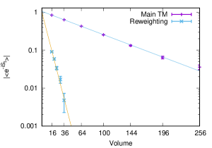
Figure 8: The average sign plotted for increasing volume at constant $\beta=2+1.4i$.

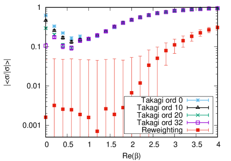
Figure 9: Absolute values of the expectation values of the phase of the reweighting factor of Eq. (35) depending on the number of included tangent spaces and $\beta$ in comparison with a standard reweighting simulation.

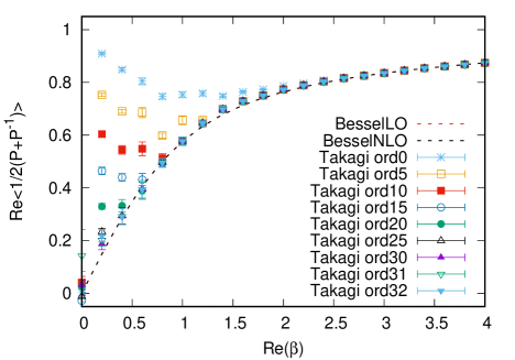
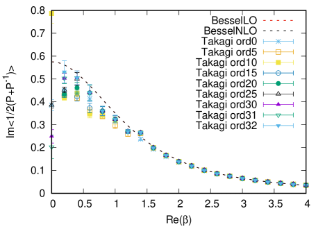
Figure 10: Takagi simulation incorporating different orders of reweighted tangent spaces on an $8\times 8$ lattice at constant $\mathrm{Im}\,(\beta)=1$. The dashed line indicates the Bessel result, see Eq. (29). Each order $k$ contains for practical reasons the $V-k$ order and all topological TMs associated with these. Shown are the real part and imaginary part of the plaquette expectation value.

III.6 Reweighting of subleading TMs

For the reweighting, the observable from Eq. (II.7) becomes

$$<\mathcal{O}>\;=$$ (35)

$$\quad\frac{<e^{-iS_{I}}\mathcal{O}+\sum_{k=1}^{n}m_{k}\det[\mathrm{d}f_{k}]e^{S_{R}-S\circ f_{k}}\mathcal{O}\circ f_{k}>_{\tau_{0}}}{<e^{-iS_{I}}+\sum_{k=1}^{n}m_{k}\det[\mathrm{d}f_{k}]e^{S_{R}-S\circ f_{k}}>_{\tau_{0}}}\,,$$

where $n$ denotes the number of subleading tangent space orders, one wants to incorporate, $m_{k}$ are the multiplicities and $f_{k}$ are linear transformations projecting the main TM $\tau_{0}$ onto the subleading tangent space $\tau_{k}$. This is done by aligning the Takagi basis using the real vectors $v_{j}$ to calculate a transformation matrix

$$\gamma^{(k)}_{ij}=(v^{(k)}_{j})^{T}v^{(0)}_{i}\,,$$ (36)

which we apply to the subleading Takagi basis

$$z^{(k)}_{i}=\sum_{j}\gamma^{(k)}_{ij}c^{(k)}_{j}v^{(k)}_{j}\,,$$ (37)

where the $c^{(k)}_{j}$ are the complex prefactors from Eq. (16). The $z^{(k)}_{i}$ are now our new aligned basis vectors for $\tau_{k}$. Therefore we can directly project from the leading to subleading tangent spaces. As already mentioned in Sec. II.7, depending on the other boundaries of the subleading tangent space, one can apply scaling factors to the variables. We observed, that for $\beta_{R},\beta_{I}\geq 0$, the main TM is always larger (or equally large) as the other subleading TMs. Instead of rescaling, we use an indicator function $\chi_{\tau_{k}}(U)$ for the boundaries: If the projected space $f_{k}(\tau_{0})=\tilde{\tau}_{k}\supseteq\tau_{k}$, then we have

$$\int_{\tau_{k}}\mathrm{d}Ug(U)=\int_{\tilde{\tau}_{k}}\mathrm{d}Ug(U)\chi_{\tau_{k}}(U)$$ (38)

with $g(U)$ an arbitrary function on the subspace. So, we simply set the integrand to zero in the reweighting process, if the projected configuration is out of bounds.

We use several symmetries to incorporate the different topological sectors for each order as well as a mapping from the $k$-th to the $(V\!\!-k)$-th TM already discussed in Sec. III.2. In the end, we have to diagonalize only $V/2$ Hessians to get every contribution. For practical reasons, we subsumed the $V/2$ TM under order $V/2-1$ and $V/2$ using a turn by $\varphi=\pi$ of the additional zero mode (33). During the reweighting process, we need to check for every contribution, if it is in its predefined boundaries, since they also differ over topological sectors (see Sec. III.3).

We applied the procedure on an $8\times 8$ lattice at constant $\mathrm{Im}\,(\beta)=1$ and compared different orders of reweighting with the BesselNLO result (see end of Sec. III.1). The results are shown in Fig. 10 as well as the average sign in Fig. 9 depending on how many orders of TMs one takes into account. The boundaries chosen are real plaquette boundaries based on the one plaquette model, since they prevent overlapping of the TMs, while allowing a large space to be explored.

IV Discussion

As we have stated already in the introduction, the particular choice of our deformation has two important advantages:

• Due to the flatness of the patches a parametrization in terms of real coordinates and basis vectors is easily constructed. It is thus straight forward to realize a sampling procedure on a particular patch. In contrast to the generalize Lefschetz thimble approach, there is no need to solve a flow equation to propose a new configuration nor to evaluate a Jacobian at each sampling point.

• Since our coordinate systems originate from a critical configuration on each patch, which is the configuration that receives the largest weight on that patch, a reweighting from one patch to another is possible without any severe overlap problem.

In the case of a pronounced hierarchy among critical configurations, we have demonstrated in the case of the 2d U(1) theory, that a well controlled approximation scheme emerges if successive contributions from suppressed patches are taken into account.

On the other hand there are two – as we believe less severe – disadvantages:

• Sampling on the flat tangential manifold rather than on the curved thimble, does not erase the sign problem completely. It would be interesting to analyze whether the optimal deformation of the original manifold, which minimizes the combined sign problem of the action on the integration domain and the one introduced by the Jacobian, is closer to the thimble decomposition or our decomposition from flat patches. We leave this for future investigations. We have demonstrated that the resulting sign problem in the case of the 2d U(1) gauge theory is, although sill exponential in volume, very mild compared to the standard reweighting procedure.

• In order to construct our deformation, we need to know all relevant critical configurations. Depending on the space-time dimension, volume and gauge group, this can be a very large amount of critical configurations.

It is one of the main results of this work that we have identified a large number of critical configurations, which are characterized by specific distributions of plaquettes across on the lattice. In particular, we have demonstrated that we can chose these critical configuration from the maximal torus of the original gauge group. We have shown further that there exists a large number of degenerate critical configurations and patches due to lattice symmetries. For the reweighting procedure we thus need to take only one of these patches into account if appropriate combinatorial multiplicity factors are used. The results look promising and systematic errors by non-homotopy vanish with growing lattice size.

We want to emphasize here that the choice of a complex coupling $\beta$ is not at all a pathological choice. In the limit of a purely imaginary coupling, the kernel of the discussed partition sum can be seen as the real time propagator of the theory. For the evaluation of real time correlation functions in a thermal bath, the Schwinger-Keldysh formalism is usually applied. Our sampling strategy might also be applied to the Schwinger-Keldysh contour, even though in this case an additional sign problem arises from the edges of the contour.

Moreover, the critical configurations we have identified here are not only critical in the case of the Yang Mills action with complex coupling $\beta$. The same configurations remain critical when we introduce fermionic matter fields with a chemical potential $\mu$. In this case the effective action might be written as

$$S_{\mathrm{eff}}(\mu;U)=\beta S_{G}(U)-\mathrm{Tr}\ln D(\mu;U)\,.$$ (39)

Hence, the action gradient is the sum of a contribution from the gauge ($S_{G}(U)$) and the fermionic part ($S_{F}(\mu;U)$) of the action. That the action gradient of the gauge part vanishes at our critical configurations has been discussed in detail above. The fermionic contribution to the gradient is given as

$$\partial_{x,\nu,a}S_{F}= \,i\,\mathrm{Tr}\Biggl{[}D^{-1}\Bigl{(}e^{\mu\delta_{\nu,0}}U_{\nu}(x)$$

$$\hskip 42.67912pt-e^{-\mu\delta_{\nu,0}}U^{\dagger}_{\nu}(x+\hat{\nu})\Bigr{)}t_{a}\Biggr{]}\,.$$ (40)

For those critical points that are not only chosen from the maximal torus of the gauge group but are also constructed from center elements of the original gauge group, the fermionic contribution vanishes as well. As all link variables are proportional to the unit matrix, the (none sparse) inverse of the fermion matrix $D^{-1}$ contains $N\times N$ diagonal blocks which are also proportional to the unit matrix. We conclude that the matrix multiplying the generator $t_{a}$ is proportional to the unit matrix and as such the whole expression vanishes. We thus hope that our strategy might also prove useful in this case, i.e. the field theoretical description of dense matter, including QCD at net-baryon number density.

V Conclusion

We have put forward here a novel nonperturbative lattice approach for Yang Mills theories with a complex gauge coupling $\beta$. The approach is based on a deformation of the original integration domain of the theory into complex space. Guided by the Lefschetz thimble decomposition of the partition sum we have chosen a new integration domain. This is constructed piecewise from patches of tangential manifolds to the relevant Lefschetz thimbles.

For the numerical implementation we have chosen to set up a Monte Carlo procedure on the main tangent space only. All further contributions from other patches are taken into account by reweighting. We have tested our approach by applying it to the case of 2d U(1) gauge theory. Here, it far out-performs our benchmark simulation with standard reweighting, see Fig. 1.

Based on this observation we plan to apply our approach to general $\mathrm{U}(N)$ and $\mathrm{SU}(N)$ gauge groups in 4d. While our approach has shown to feature an exponentially better performance than standard reweighting, it remains to be shown that the sign problem stays numerically manageable also in these cases. We hope to address these questions in a forthcoming publication. Moreover, we envisage simulations of fermionic matter fields at finite chemical potential as well as real-time lattice theories with expectation values along the Schwinger-Keldysh contour.

Appendix A General complex Hessians

If we can not write the Hessian as $H=\beta M$, with a real matrix $M$ as in Sec. II.4, we consider real and imaginary parts of the Takagi Eq. (14) separately (see e.g. Alexandru et al. (2016a))

$$(H^{R}-iH^{I})(v^{R}-iv^{I})=\lambda(v^{R}+iv^{I})\\[4.30554pt] \Leftrightarrow\begin{pmatrix}H^{R}&-H^{I}\\ -H^{I}&-H^{R}\end{pmatrix}\begin{pmatrix}v^{R}\\ v^{I}\end{pmatrix}=\lambda\begin{pmatrix}v^{R}\\ v^{I}\end{pmatrix}\;.$$ (41)

The matrix is by definition symmetric and we have only real eigenvalues, positive $\lambda$ for Takagi and negative $\lambda$ for Anti-Takagi vectors. The zero modes span again the whole critical manifold. Since for compact gauge groups, we are only interested in the real subspace, which are naturally compact. Therefore, we impose $v^{I}=0$ and get

$$H^{R}v^{R}=0\;\;\text{and}\;\;H^{I}v^{R}=0\;.$$ (42)

This implies that the critical manifold is spanned by the mutual zero modes of the real and imaginary part of the Hessian. The strategy therefore is to calculate the zero modes either parts and test, if these are also zero modes of the other part. The number of real zero modes and of the Takagis have to add up to the overall dimension.

Appendix B The toron formulation

We reformulate the theory as mentioned in Eq. (24). Then we gauge all time-like directions into one link. This reduces the degrees of freedom by $N_{x}(N_{t}-1)$.

Next, we define new lattice variables $\theta$ and express the links (in their algebra representation $\phi_{\mu}(x,t)$) in terms of these. Thereto we write direction vectors ($\vec{\varphi}(x,t),\vec{\varphi}_{2}(x),\vec{\varphi}_{1}(0)$) in link space indicating how the new variables change the links in their respective direction. This yields the following parametrization

$$\phi_{\mu}(y,t) =\sum_{(x,\tau)\neq(0,0)}\theta(x,\tau)(\vec{\varphi}(x,\tau))_{\phi_{\mu}(y,t)}$$ (43)

$$+\sum_{x}\theta_{2}(x)(\vec{\varphi}_{2}(x))_{\phi_{\mu}(y,t)}+\theta_{1}(0)(\vec{\varphi}_{1}(0))_{\phi_{\mu}(y,t)}$$

for each remaining link. The $\theta(x,t)$ shall denote plaquette variables, while the $\theta_{2}(x)$ and $\theta_{1}(0)$ denote zero modes at space slices or the zero time slice. We will integrate them out later. All space-like links can be replaced by plaquette variables

$$\vec{\varphi}(x,t) =\hat{\phi}_{1}(x,t\mod N_{t})-\hat{\phi}_{1}(x,t-1\mod N_{t})\,,$$

$$t\in\{2,\ldots,N_{t}\}\,,$$ (44)

and a zero mode

$$\vec{\varphi}_{2}(x)=\sum_{t=0}^{N_{t}-1}\hat{\phi}_{1}(x,t)\,,$$

for each space slice. We use the notation $\hat{\phi}$ to denote a unit vector in link space corresponding to the variable $\phi$.

We have $V$ variables, which are linear independent, since we can express each space-like link by

$$\hat{\phi}_{1}(x,t)=\frac{1}{N_{t}}\Big{(}\vec{\varphi}_{2}(x) +\sum_{k=1}^{(t-1)\mod N_{t}}k\vec{\varphi}(x,k)$$ (45)

$$-\sum_{l=1}^{(-t)\mod N_{t}}l\vec{\varphi}(x,N_{t}-l)\Big{)}\,.$$

We replace the remaining $N_{x}$ time-like links with plaquette variables

$$\vec{\varphi}(x,0) =\hat{\phi}_{2}(x,0)+\hat{\phi}_{1}(x,1)$$ (46)

$$-\hat{\phi}_{2}(x+1\mod N_{x},0)-\hat{\phi}_{1}(x,0)\,,$$

for $x\in\{1,\ldots,N_{x}-1\}$ and the zero mode

$$\vec{\varphi}_{1}(0)=\sum_{x=0}^{N_{x}-1}\hat{\phi}_{2}(x,0)\,.$$

Using the fact that we already have a basis transform for the space-like links, we can express the remaining time-like links in terms of these variables in a similar fashion to Eq. (45). This proves that our variable transformation is invertible and therefore we have a non-zero Jacobian. By the parametrization (43) and the toron action (24), we rewrite the partition sum to

$$Z\;=\;\int\mathrm{d}\theta_{1}(0)\prod_{x}\mathrm{d}\theta_{2}(x)\prod_{(x,t)\neq(0,0)}\mathrm{d}\theta(x,t)\det\left[\frac{\partial\vec{\phi}}{\partial\vec{\theta}}\right]$$

$$\;\times\;\exp\left[\beta/2\sum_{(x,t)\neq(0,0)}\left(e^{i\theta(x,t)}+e^{-i\theta(x,t)}\right)\right]$$ (47)

$$\;\times\;\exp\left[\beta/2\left(e^{-i\sum_{(x,t)\neq(0,0)}\theta(x,t)}+e^{i\sum_{(x,t)\neq(0,0)}\theta(x,t)}\right)\right]\,.$$

Since our transformation is linear, the Jacobian $\det\left[\frac{\partial\vec{\phi}}{\partial\vec{\theta}}\right]$ is constant and drops out when taking expectation values. The same is true for the integrals over the zero modes. They do not change the plaquettes and the action. Their contribution is given by a constant factor. Therefore they can be dropped without changing expectation values. This reduces our degrees of freedom by $N_{x}+1$ to $V-1$. The remaining effective degrees of freedom $\theta(x,t)$ are called toron variables.

Appendix C A local update procedure for a 2-dimensional $\mathrm{U}(1)$ gauge theory

We parametrize this tangent space by arclength. Therefore, we have

$$\varphi_{\mu}(x)=\sqrt{\frac{\beta^{*}}{|\beta|}}\lambda_{\mu}(x)\;,$$ (48)

where $\lambda_{\mu}(x)\in\mathbb{R}$. We limit this space by the intersections seen in the one plaquette model (see Sec. II.4). Therefore we have

$$\Lambda(x) \;=\;\lambda_{0}(x)+\lambda_{1}(x+\hat{0})-\lambda_{0}(x+\hat{1})-\lambda_{1}(x)$$

$$\;\in\;[-\pi R,+\pi R]\;,\quad\text{with}\quad R=\mathrm{Re}\;\sqrt{\frac{\beta^{*}}{|\beta|}}\;.$$ (49)

We enforce this limit by setting the probability for proposed configurations outside this limits to zero, effectively rejecting them in the Metropolis step. The algorithm is according to that

1. Go through the lattice by a checker board pattern and pick accordingly $\lambda_{\mu}(x)$.

2. Make a proposal $\Delta\lambda_{\mu}(x)\sim\mathrm{Gauss}(\mu=0,\sigma)$. and calculate the two adjacent plaquettes $\Lambda(x)$, $\Lambda(x-\hat{\nu})$ with $\nu\neq\mu$.

3. If $\Lambda(x)$ and/or $\Lambda(x-\hat{\nu})$ is not within the boundaries, set $e^{-S^{\prime}}=0$. Otherwise calculate the change of the action $\Delta S(P_{01}(x),P_{01}(x-\hat{\nu}))$

4. Do a Metropolis Accept/Reject step and begin again from 1.

Since our links can wander off into the imaginary direction, we perform gauge cooling steps, see i.e. Seiler et al. (2013). Locally for a site $x$ we can analytically compute an optimum for the gauge transformation $V(x)$. Therefore we look at the unitarity norm

$$\mathcal{F}[U_{\mu}(x)]\;=$$ (50)

$$\quad\sum_{x,\mu}\mathrm{Tr}\left[U^{\dagger}_{\mu}(x)U_{\mu}(x)+(U^{\dagger}_{\mu}(x))^{-1}U^{-1}_{\mu}(x)-2\mathbb{I}\right]\;,$$

which simplifies in our case $U_{\mu}(x)=e^{i\phi_{\mu}(x)}$ to

$$\mathcal{F}[\phi_{\mu}(x)] =\sum_{x,\mu}\left[e^{-2\phi^{I}_{\mu}(x)}+e^{2\phi^{I}_{\mu}(x)}-2\right]$$

$$=\sum_{x,\mu}\left[|U_{\mu}(x)|^{-2}+|U_{\mu}(x)|^{2}-2\right]\;,$$ (51)

depending only on the absolute value of the links. How a gauge transformation changes (50) depends therefore only on its absolute value. For a local $V(x)$ we get the local minimum at

$$|V(x)|=\sqrt[4]{\frac{\sum_{\mu}\left(|U_{\mu}(x)|^{-2}+|U_{\mu}(x-\hat{\mu})|^{2}\right)}{\sum_{\mu}\left(|U_{\mu}(x)|^{2}+|U_{\mu}(x-\hat{\mu})|^{-2}\right)}},$$ (52)

which we apply between sweeps.
Alternatively one doesn’t need to record the link values and we restrict ourselves to just recording the plaquette values, which are naturally bounded. We apply the update steps only in terms of changes in links affecting their neighboring plaquettes.
Reweighting to different orders of TMs can also be applied here by injectively mapping the plaquette configurations to link configurations and aligning the TMs bases to the unit basis, corresponding to the individual links. Given a set of plaquette values $\theta(x,t)$ in the algebra, a possible mapping to link variables $\phi_{\mu}(x,t)$ would be

1. For $x=0$ and all $t\in 0,\ldots,N_{t}-1$ set

   $$\phi_{2}(0,t)=\theta(0,t).$$

2. For $x=1$, all $t$, set

   $$\phi_{2}(2,t)=-\theta(1,t).$$

3. Successively for $x\in 2,\ldots,N_{x}-2$ and all $t$, set

   $$\phi_{2}(x+1,t)=\phi_{2}(x,t)-\theta(x,t).$$

4. The last space-slice $x=N_{x}-1$ is assigned successively by setting the first space-like link $\phi_{1}(x,0)=0$ and for $t\in 1,\ldots,N_{t}-1$ to

   $$\phi_{1}(x,t)=\phi_{1}(x,t-1)+\theta(x,t-1)+\phi_{2}(0,t-1)-\phi_{2}(x,t-1).$$

The last plaquette value $\theta(N_{x}-1,N_{t}-1)$ is automatically taken into account up to a factor of $2\pi$ by the periodic boundary conditions. Now the values obtained for the algebra of the links are used to map onto the subleading TMs.

Appendix D Proof of the matrix identity

We consider the system of equations

$$\mathrm{Tr}[MT^{a}]=0\;\forall a,$$ (53)

where $M$ is a general $N\times N$ complex matrix and $T^{a}$ are generators of the lie algebra $\mathfrak{su}(N)$ or $\mathfrak{u}(N)$. We show that Eq. (53) holds, iff $M=c\mathbbm{1}$ for an arbitrary $c\in\mathbb{C}$ for $\mathfrak{su}(N)$ and $M=0$ for $\mathfrak{u}(N)$.
First note, that the $T^{a}$ also form the basis of the complex lie algebras $\mathfrak{sl}(N,\mathbb{C})$, $\mathfrak{gl}(N,\mathbb{C})$. This is done by allowing complex coefficients effectively removing the anti-hermiticity of the elements. Consequently elements are only defined by being traceless for $\mathfrak{sl}(N,\mathbb{C})$ and we have $\mathfrak{gl}(N,\mathbb{C})\simeq\mathbb{C}^{N\times N}$.
The statement does not depend on the basis of the Lie algebra: Let $T^{a}$ and $S^{a}$ be two basis of the same Lie algebra. We show that

$$\mathrm{Tr}[MT^{a}]=0\;\forall a\;\Leftrightarrow\;\mathrm{Tr}[MS^{a}]=0\;\forall a\;$$ (54)

by expanding $S^{a}=\sum_{b}c^{a}_{b}T^{b}$ and using the linearity of the trace

$$\mathrm{Tr}[MS^{a}]=\sum_{b}c^{a}_{b}\mathrm{Tr}[MT^{b}]=0.$$ (55)

Especially the statement is equivalent to

$$\mathrm{Tr}[MT]=0\;\forall T\in\mathfrak{sl}(N,\mathbb{C})\;\text{or}\;\forall T\in\mathfrak{gl}(N,\mathbb{C}).$$ (56)

Note, that the backward direction is trivial, since $\mathrm{Tr}[c\mathbbm{1}T]=c\mathrm{Tr}[T]=0$ for $T$ being traceless and $\mathrm{Tr}[0T]=\mathrm{Tr}[0]=0$ for $T\in\mathfrak{gl}(N,\mathbb{C})$.
For the forward direction we use the more general statement (56). For $T\in\mathfrak{sl}(N,\mathbb{C})$, suppose first $M_{ij}\neq 0$ for $i\neq j$. Then we can choose $T_{lk}=\delta_{lj}\delta_{ki}$, which is obviously traceless and have

$$\mathrm{Tr}[MT]= \sum_{k,l}M_{kl}T_{lk}=\sum_{k,l}M_{kl}\delta_{lj}\delta_{ki}$$

$$= M_{ij}\neq 0.$$ (57)

For $M_{ii}\neq M_{jj},\;i\neq j$ we take $T_{lk}=\delta_{li}\delta_{ki}-\delta_{lj}\delta_{kj}$, which is also traceless and have

$$\mathrm{Tr}[MT]= \sum_{k,l}M_{kl}T_{lk}=\sum_{k,l}M_{kl}(\delta_{li}\delta_{ki}-\delta_{lj}\delta_{kj})$$

$$= M_{ii}-M_{jj}\neq 0.$$ (58)

Since $i$ and $j$ were arbitrary $M=c\mathbbm{1}$ for some $c\in\mathbb{C}$.
For $T\in\mathfrak{gl}(N,\mathbb{C})\sup\mathfrak{sl}(N,\mathbb{C})$, $T$ is not traceless anymore and can also be e.g. $\mathbbm{1}$, which excludes the $M=c\mathbbm{1}$ case and $M$ has to be zero to fulfill the statement.

References

- Barbour et al. (1998) I. M. Barbour, S. E. Morrison, E. G. Klepfish, J. B. Kogut, and M.-P. Lombardo, Nucl. Phys. B Proc. Suppl. 60A, 220 (1998), arXiv:hep-lat/9705042 .
- Fodor and Katz (2002) Z. Fodor and S. Katz, Phys. Lett. B 534, 87 (2002), arXiv:hep-lat/0104001 .
- Allton et al. (2002) C. Allton, S. Ejiri, S. Hands, O. Kaczmarek, F. Karsch, E. Laermann, C. Schmidt, and L. Scorzato, Phys. Rev. D 66, 074507 (2002), arXiv:hep-lat/0204010 .
- Allton et al. (2003) C. Allton, S. Ejiri, S. Hands, O. Kaczmarek, F. Karsch, E. Laermann, and C. Schmidt, Phys. Rev. D 68, 014507 (2003), arXiv:hep-lat/0305007 .
- Gavai and Gupta (2003) R. V. Gavai and S. Gupta, Phys. Rev. D 68, 034506 (2003), arXiv:hep-lat/0303013 .
- de Forcrand and Philipsen (2002) P. de Forcrand and O. Philipsen, Nucl. Phys. B 642, 290 (2002), arXiv:hep-lat/0205016 .
- D’Elia and Lombardo (2003) M. D’Elia and M.-P. Lombardo, Phys. Rev. D 67, 014505 (2003), arXiv:hep-lat/0209146 .
- Kratochvila and de Forcrand (2004) S. Kratochvila and P. de Forcrand, Prog. Theor. Phys. Suppl. 153, 330 (2004), arXiv:hep-lat/0309146 .
- Alexandru et al. (2005) A. Alexandru, M. Faber, I. Horvath, and K.-F. Liu, Phys. Rev. D 72, 114513 (2005), arXiv:hep-lat/0507020 .
- Karsch and Mutter (1989) F. Karsch and K. Mutter, Nucl. Phys. B 313, 541 (1989).
- de Forcrand et al. (2014) P. de Forcrand, J. Langelage, O. Philipsen, and W. Unger, Phys. Rev. Lett. 113, 152002 (2014), arXiv:1406.4397 [hep-lat] .
- Gattringer and Langfeld (2016) C. Gattringer and K. Langfeld, Int. J. Mod. Phys. A 31, 1643007 (2016), arXiv:1603.09517 [hep-lat] .
- Gagliardi and Unger (2020) G. Gagliardi and W. Unger, Phys. Rev. D 101, 034509 (2020), arXiv:1911.08389 [hep-lat] .
- Ambjorn et al. (2002) J. Ambjorn, K. Anagnostopoulos, J. Nishimura, and J. Verbaarschot, JHEP 10, 062 (2002), arXiv:hep-lat/0208025 .
- Fodor et al. (2007) Z. Fodor, S. D. Katz, and C. Schmidt, JHEP 03, 121 (2007), arXiv:hep-lat/0701022 .
- Langfeld et al. (2016) K. Langfeld, B. Lucini, R. Pellegrini, and A. Rago, Eur. Phys. J. C 76, 306 (2016), arXiv:1509.08391 [hep-lat] .
- Karsch and Wyld (1985) F. Karsch and H. Wyld, Phys. Rev. Lett. 55, 2242 (1985).
- Aarts et al. (2010) G. Aarts, E. Seiler, and I.-O. Stamatescu, Phys. Rev. D 81, 054508 (2010), arXiv:0912.3360 [hep-lat] .
- Aarts et al. (2013) G. Aarts, F. A. James, J. M. Pawlowski, E. Seiler, D. Sexty, and I.-O. Stamatescu, JHEP 03, 073 (2013), arXiv:1212.5231 [hep-lat] .
- Sexty (2014) D. Sexty, Phys. Lett. B 729, 108 (2014), arXiv:1307.7748 [hep-lat] .
- Attanasio et al. (2020) F. Attanasio, B. Jäger, and F. P. Ziegler, Eur. Phys. J. A 56, 251 (2020), arXiv:2006.00476 [hep-lat] .
- Pham (1983) F. Pham, Proc. Symp. pure Math 40, 319 (1983).
- Witten (2010) E. Witten, (2010), arXiv:1009.6032 [hep-th] .
- Cristoforetti et al. (2012) M. Cristoforetti, F. Di Renzo, and L. Scorzato (AuroraScience), Phys. Rev. D86, 074506 (2012), arXiv:1205.3996 [hep-lat] .
- Alexandru et al. (2020) A. Alexandru, G. Basar, P. F. Bedaque, and N. C. Warrington, (2020), arXiv:2007.05436 [hep-lat] .
- Cristoforetti et al. (2014) M. Cristoforetti, F. Di Renzo, G. Eruzzi, A. Mukherjee, C. Schmidt, L. Scorzato, and C. Torrero, Phys. Rev. D 89, 114505 (2014), arXiv:1403.5637 [hep-lat] .
- Alexandru et al. (2017a) A. Alexandru, G. Basar, P. F. Bedaque, and G. W. Ridgway, Phys. Rev. D 95, 114501 (2017a), arXiv:1704.06404 [hep-lat] .
- Bursa and Kroyter (2018) F. Bursa and M. Kroyter, JHEP 12, 054 (2018), arXiv:1805.04941 [hep-lat] .
- Mori et al. (2017) Y. Mori, K. Kashiwa, and A. Ohnishi, Phys. Rev. D96, 111501 (2017), arXiv:1705.05605 [hep-lat] .
- Mori et al. (2018) Y. Mori, K. Kashiwa, and A. Ohnishi, PTEP 2018, 023B04 (2018), arXiv:1709.03208 [hep-lat] .
- Alexandru et al. (2017b) A. Alexandru, P. F. Bedaque, H. Lamm, and S. Lawrence, Phys. Rev. D 96, 094505 (2017b), arXiv:1709.01971 [hep-lat] .
- Wynen et al. (2020) J.-L. Wynen, E. Berkowitz, S. Krieg, T. Luu, and J. Ostmeyer, (2020), arXiv:2006.11221 [cond-mat.str-el] .
- Alexandru et al. (2017c) A. Alexandru, G. Basar, P. F. Bedaque, and N. C. Warrington, Phys. Rev. D 96, 034513 (2017c), arXiv:1703.02414 [hep-lat] .
- Fukuma et al. (2019) M. Fukuma, N. Matsumoto, and N. Umeda, Phys. Rev. D 100, 114510 (2019), arXiv:1906.04243 [cond-mat.str-el] .
- Di Renzo and Eruzzi (2018) F. Di Renzo and G. Eruzzi, Phys. Rev. D 97, 014503 (2018), arXiv:1709.10468 [hep-lat] .
- Bluecher et al. (2018) S. Bluecher, J. M. Pawlowski, M. Scherzer, M. Schlosser, I.-O. Stamatescu, S. Syrkowski, and F. P. Ziegler, SciPost Phys. 5, 044 (2018), arXiv:1803.08418 [hep-lat] .
- Di Renzo et al. (2020) F. Di Renzo, S. Singh, and K. Zambello, (2020), arXiv:2008.01622 [hep-lat] .
- Alexandru et al. (2016a) A. Alexandru, G. Basar, and P. Bedaque, Phys. Rev. D93, 014504 (2016a), arXiv:1510.03258 [hep-lat] .
- Wilson (1974) K. G. Wilson, Phys. Rev. D10, 2445 (1974).
- Cristoforetti et al. (2013) M. Cristoforetti, F. Di Renzo, A. Mukherjee, and L. Scorzato, Phys. Rev. D88, 051501 (2013), arXiv:1303.7204 [hep-lat] .
- Fujii et al. (2013) H. Fujii, D. Honda, M. Kato, Y. Kikukawa, S. Komatsu, and T. Sano, JHEP 10, 147 (2013), arXiv:1309.4371 [hep-lat] .
- Alexandru et al. (2016b) A. Alexandru, G. Basar, P. F. Bedaque, G. W. Ridgway, and N. C. Warrington, JHEP 05, 053 (2016b), arXiv:1512.08764 [hep-lat] .
- Witten (2011) E. Witten, AMS/IP Stud. Adv. Math. 50, 347 (2011), arXiv:1001.2933 [hep-th] .
- Lüscher (2010) M. Lüscher, JHEP 08, 071 (2010), [Erratum: JHEP 03, 092 (2014)], arXiv:1006.4518 [hep-lat] .
- Kanwar et al. (2020) G. Kanwar, M. S. Albergo, D. Boyda, K. Cranmer, D. C. Hackett, S. Racanière, D. J. Rezende, and P. E. Shanahan, Phys. Rev. Lett. 125, 121601 (2020), arXiv:2003.06413 [hep-lat] .
- Boyda et al. (2020) D. Boyda, G. Kanwar, S. Racanière, D. J. Rezende, M. S. Albergo, K. Cranmer, D. C. Hackett, and P. E. Shanahan, (2020), arXiv:2008.05456 [hep-lat] .
- Seiler et al. (2013) E. Seiler, D. Sexty, and I.-O. Stamatescu, Phys. Lett. B723, 213 (2013), arXiv:1211.3709 [hep-lat] .
- Hirasawa et al. (2020) M. Hirasawa, A. Matsumoto, J. Nishimura, and A. Yosprakob, JHEP 09, 023 (2020), arXiv:2004.13982 [hep-lat] .
- Kashiwa and Mori (2020) K. Kashiwa and Y. Mori, Phys. Rev. D 102, 054519 (2020), arXiv:2007.04167 [hep-lat] .
- Balian et al. (1974) R. Balian, J. M. Drouffe, and C. Itzykson, Phys. Rev. D10, 3376 (1974), [,74(1974)].
- Migdal (1975) A. A. Migdal, Sov. Phys. JETP 42, 413 (1975), [,114(1975)].
- Milnor et al. (1969) J. Milnor, M. SPIVAK, and R. WELLS, Morse Theory. (AM-51), Volume 51 (Princeton University Press, 1969).