Accurate error estimation in CG

Abstract

In practical computations, the (preconditioned) conjugate gradient (P)CG method is the iterative method of choice for solving systems of linear algebraic equations $Ax=b$ with a real symmetric positive definite matrix $A$. During the iterations it is important to monitor the quality of the approximate solution $x_{k}$ so that the process could be stopped whenever $x_{k}$ is accurate enough. One of the most relevant quantities for monitoring the quality of $x_{k}$ is the squared $A$-norm of the error vector $x-x_{k}$. This quantity cannot be easily evaluated, however, it can be estimated. Many of the existing estimation techniques are inspired by the view of CG as a procedure for approximating a certain Riemann–Stieltjes integral. The most natural technique is based on the Gauss quadrature approximation and provides a lower bound on the quantity of interest. The bound can be cheaply evaluated using terms that have to be computed anyway in the forthcoming CG iterations. If the squared $A$-norm of the error vector decreases rapidly, then the lower bound represents a tight estimate. In this paper we suggest a heuristic strategy aiming to answer the question of how many forthcoming CG iterations are needed to get an estimate with the prescribed accuracy. Numerical experiments demonstrate that the suggested strategy is efficient and robust.

15A06, 65F10

1 Introduction

Nowadays, the (preconditioned) conjugate gradient (P)CG method of Hestenes and Stiefel [11] is the method of choice for solving large and sparse systems of linear algebraic equations

(1) $$Ax=b$$

with a real symmetric positive definite matrix $A$ of order $n$. In theory, the CG method has the best of the two worlds of iterative and direct linear solvers. As an iterative method, it has low memory requirements and provides an approximate solution $x_{k}$ at each iteration allowing to stop the algorithm whenever a stopping criterion is met. As a direct method, it finds (assuming exact arithmetic) the solution after at most $n$ iterations, and the approximate solution $x_{k}$ is optimal in the sense that it minimizes the squared $A$-norm (also called the energy norm) of the error vector $x-x_{k}$,

(2) $$\varepsilon_{k}\equiv\|x-x_{k}\|_{A}^{2}=(A(x-x_{k}),x-x_{k}),$$

over the underlying linear manifold. Note that $\left\|x-y\right\|_{A}^{2}$ as a function of $y$ was called “the error function” in the original Hestenes and Stiefel paper [11]. The authors mention [11, p. 413] that this function can be used as a measure of the “goodness” of $x_{k}$ as an approximation of $x$. Following them and for the sake of simplicity, we will call $\varepsilon_{k}$ the error. In the context of solving various real word problems, the error $\varepsilon_{k}$ has an important meaning, e.g., in physics, quantum chemistry, or mechanics, and plays a fundamental role in evaluating convergence and estimating the algebraic error in the context of numerical solving of PDE’s [1, 12, 2, 3].

The theoretical properties of CG can be described in many mathematically equivalent ways. For example, the connection with orthogonal polynomials, which has already been noticed in [11], allows seeing CG as a procedure for computing Gauss quadrature approximation to a Riemann–Stieltjes integral. This view of CG is very useful not only for estimating norms of the error vectors, but also for analyzing the CG behavior in finite precision arithmetic. During many finite precision CG computations, the orthogonality among the residual vectors is usually lost quickly and convergence is delayed [9, 10]. Based on previous results of Paige [20], it has been shown by Greenbaum [9] that the results of finite precision CG computations can be interpreted (up to some small inaccuracy) as results of exact CG applied to a larger system with a system matrix having many eigenvalues distributed throughout tiny intervals around the eigenvalues of $A$. In other words, the results of [9] show that some theoretical properties of CG remain valid even in finite precision arithmetic. For a summary of the properties of the CG and Lanczos algorithms in finite precision arithmetic see, e.g., [16, 17].

Inspired by the connection of CG with Riemann–Stieltjes integrals, a way of research on estimating norms of the error vector was started by Gene Golub in the 1970s and continued throughout the years with several collaborators (e.g., G. Dahlquist, S. Eisenstat, S. Nash, B. Fischer, G. Meurant, Z. Strakoš). The main idea is to approximate the Riemann–Stieltjes integral of a suitable function by a Gauss or another modified quadrature rule (Gauss–Radau, Gauss–Lobatto, anti-Gauss etc.), and try to bound the estimated quantity [6, 8, 7]. Note that the resulting bounds can sometimes be very inaccurate approximations to the quantity of interest.

As already mentioned above, the error $\varepsilon_{k}$ must play a prominent role in evaluating CG convergence. In this paper we concentrate on its accurate estimation. Following the ideas of [8, 7, 21, 18, 19], one can improve the accuracy of the bounds, considering quadrature rules at iterations $k$ and $k+d$ for some integer $d\geq 0$ called the delay. At CG iteration $k+d$, an improved estimate of the error at iteration $k$ is obtained. For a detailed construction of the (lower and upper) bounds on $\varepsilon_{k}$ based on the delay approach see, e.g., [18, Section 2.5]. The larger the delay is, the better are the bounds at iteration $k$. However, a constant value of $d$ is usually not sufficient in the initial stage of convergence, and it may require too many extra steps of CG in the convergence phase. Hence, there is a need for developing a heuristic technique to choose $d$ adaptively at each iteration, to reflect the required accuracy of the estimate.

In this paper, we focus on estimating the error $\varepsilon_{k}$ using the Gauss quadrature approach that provides a lower bound. We address the problem of the adaptive choice of $d$. In particular, we develop an adaptive (heuristic) strategy, which aims to ensure that the lower bound approximates the error $\varepsilon_{k}$ with a prescribed tolerance. Note that an analogous technique can be also used to improve the accuracy of other bounds based, e.g., on Gauss–Radau quadrature.

The paper is organized as follows. In Section 2 we introduce the notation, recall the standard Hestenes and Stiefel version of the CG algorithm, and present formulas that will be used for constructing the lower bound of the error. In Section 3, we describe an adaptive strategy for choosing the delay $d$, aiming to meet the prescribed accuracy of the lower bound. Section 4 shows how to modify the formulas for preconditioned CG. Some possible extensions to make the adaptive strategy more reliable in hard cases are presented in Section 5. Results of numerical experiments are given in Section 6 and the paper ends with a concluding discussion. In Appendix A we provide a simplified MATLAB code of the suggested algorithm.

2 The CG algorithm and the lower bound on the error

Algorithm 1 Conjugate Gradients

  input $A$, $b$, $x_{0}$

  $r_{0}=b-Ax_{0}$, $p_{0}=r_{0}$

  for $k=0,\dots$ until convergence do

     $\alpha_{k}=\frac{r_{k}^{T}r_{k}}{p_{k}^{T}Ap_{k}}$

     $x_{k+1}=x_{k}+\alpha_{k}p_{k}$

     $r_{k+1}=r_{k}-\alpha_{k}Ap_{k}$              $\left.\begin{array}[]{@{}c@{}}\\ {}\hfil\\ {}\hfil\\ {}\hfil\\ {}\hfil\\ {}\hfil\end{array}\right\}\begin{tabular}[]{l}{\tt cgiter(k)}\end{tabular}$

     $\beta_{k+1}=\frac{r_{k+1}^{T}r_{k+1}}{r_{k}^{T}r_{k}}$

     $p_{k+1}=r_{k+1}+\beta_{k+1}p_{k}$

  end for

The classical version of the Conjugate Gradient method (Hestenes and Stiefel, [11]) is given by Algorithm 1. For later use, we denote the function that performs one CG iteration for updating the approximations $x_{k}$, corresponding residuals $r_{k}$, direction vectors $p_{k}$, and computing the CG coefficients $\alpha_{k}$ and $\beta_{k+1}$ by cgiter(k).

The theoretical properties of CG are well known and we do not list them here; see, for instance, [16]. In our context it is only important that the sequence of errors $\{\varepsilon_{k}\}$ is decreasing and that the value of the difference between two consecutive terms is known. The proof of results of the following lemma can be found in standard literature; see, e.g., [8, 16, 21].

Lemma 2.1.

Until the solution is found, i.e., $x_{s}=x$, it holds that

(3) $$\varepsilon_{k}=\alpha_{k}\|r_{k}\|^{2}+\varepsilon_{k+1},\qquad k=0,1,\ldots,s-1,$$

with $\alpha_{k}\|r_{k}\|^{2}>0$, $k=0,1,\ldots,s-1$. In particular, the squared $A$-norm of the error vector $x-x_{k}$ in CG is decreasing, i.e.,

(4) $$\varepsilon_{k}>\varepsilon_{k+1},\qquad k=0,1,\ldots,s-1.$$

Note that Lemma 2.1 assumes exact arithmetic so that the algorithm always finds the exact solution, i.e., $x_{s}=x$ for some $s\leq n$. In finite precision computations, the errors $\varepsilon_{k}$ usually do not approach zero, but reach an ultimate level of accuracy proportional to the squared machine precision, and then, they stagnate. Nevertheless, it has been shown in [21] that until the ultimate level of accuracy is reached, the identity (3) and the inequality (4) hold also for the computed quantities, up to some small inaccuracy. Hence, considering iterations $k$ before this level is reached, we can assume that (3) and (4) do hold also during finite precision computations.

The relation (3) is the basis for the derivation of the lower bound on the error. Given a nonnegative integer $d$ and assuming that (3) holds for iterations $k$, $k+1$, $\dots$, $k+d$, with $k+d\leq s-1$, we obtain

(5) $$\varepsilon_{k}\;=\;\sum^{k+d}_{j=k}\alpha_{j}\|r_{j}\|^{2}\;+\;\varepsilon_{k+d+1}\,,$$

see [21], and we define

(6) $$\Delta_{k:k+d}\equiv\sum^{k+d}_{j=k}\alpha_{j}\|r_{j}\|^{2}.$$

Note that instead of $\Delta_{k:k}$ we write $\Delta_{k}$. Using the fact that $\varepsilon_{k+d+1}\geq 0$, the quantity (6) represents a lower bound on $\varepsilon_{k}$. The indisputable advantage of the bound (6) is that it is very cheap to compute since it only involves quantities which have to be computed in CG, and, as already mentioned, it works under natural assumptions also for finite precision computations; for more details see [21].

While (5) suggests that the computable lower bound (6) is tight for sufficiently large $d$, the choice of $d$ that ensures a sufficient accuracy of the lower bound in practical computations, is usually unknown. A constant value of $d$ can be fine in some special cases with a rapid and linear convergence. However, in general, we expect that the convergence of the $A$-norm of the error vector $x-x_{k}$ in (P)CG is irregular. Quasi-stagnation can alternate with convergence periods, and in a convergence period we can often observe linear, superlinear, but also sublinear convergence.

To illustrate numerically the behavior of the bound $\Delta_{k:k+d}^{\scriptscriptstyle 1/2}$, we consider the matrix s3dkq4m2 of order $n=90449$ that can be downloaded from the SuiteSparse Matrix collection. The right-hand side vector $b$ is randomly generated and normalized to $1$. The factor $L$ in the preconditioner $M=LL^{T}$ is determined by the MATLAB incomplete Cholesky (ichol) factorization with threshold dropping, type = ’ict’, droptol = 1e-5, and with the global diagonal shift diagcomp = 1e-2.

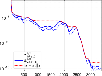
Figure 1: Matrix s3dkq4m2: the $A$-norm of the error vector $x-x_{k}$ (dotted curve) and the lower bound $\Delta_{k:k+d}^{\scriptscriptstyle 1/2}$ for two fixed values of $d$: $d=10$ (solid curve) and $d=100$ (thick solid curve).

In Figure 1 we can observe that $\|x-x_{k}\|_{A}$ (dotted curve) exhibits an irregular behaviour. The lower bound $\Delta_{k:k+d}^{\scriptscriptstyle 1/2}$ for $d=10$ (solid curve) underestimates significantly the quantity of interest in the case of quasi-stagnation, but, when convergence starts around iteration 2500, the lower bound $\Delta_{k:k+d}^{\scriptscriptstyle 1/2}$ is sufficiently accurate. The choice $d=100$ (thick solid curve) improves the results, but $\|x-x_{k}\|_{A}$ is still underestimated by several orders of magnitude. However, in the final convergence phase we now use a value of $d$ larger than necessary, and, therefore, we waste computational resources, particularly, if the error is used as a criterion to stop the iterations. One may think that we do not have to care too much about the quasi-stagnation phase, but if the underestimation of the $A$-norm of the error is too large, we may undesirably stop the iterations too soon when we are far of having a good approximation of the solution.

This example demonstrates clearly a need for developing a technique to choose $d$ adaptively. As we said, if our stopping criterion is based on the lower bound (6) and $d$ is too small, we are at risk to stop the iterations too early. At the same time, we would like to keep $d$ as small as possible to avoid unnecessary iterations. This is a nontrivial task. As we will see later, we can never guarantee a completely safe choice of $d$. Nevertheless, we are able to suggest a strategy that works satisfactorily in most cases.

3 The adaptive choice of $d$

In this section we set a requirement on the accuracy of the bound, introduce the ideal value of $d$, which ensures this accuracy, and present a first adaptive strategy for the choice of $d$.

3.1 Prescribing the accuracy of the estimate

Given a prescribed tolerance $\tau\in(0,1)$, we require that the relative error of the lower bound satisfies

(7) $$\frac{\varepsilon_{k}-\Delta_{k:k+d}}{\varepsilon_{k}}\leq\tau.$$

By simple manipulations, this is equivalent to

(8) $$\varepsilon_{k}\leq\frac{\Delta_{k:k+d}}{1-\tau}.$$

In other words, if (7) holds, then we also get an upper bound on the error. We observe that the relative error of the upper bound (8) is bounded above by $\tau/(1-\tau)$. Note also that if (7) holds, then

(9) $$\frac{\|x-x_{k}\|_{A}-\Delta_{k:k+d}^{1/2}}{\|x-x_{k}\|_{A}}<\tau,$$

i.e., the $A$-norm $\|x-x_{k}\|_{A}=\varepsilon_{k}^{1/2}$ is approximated by $\Delta_{k:k+d}^{1/2}$ with a relative accuracy less than $\tau$.

Using (5), one can rewrite (7) as

(10) $$\frac{\varepsilon_{k+d+1}}{\varepsilon_{k}}\leq\tau.$$

It means that $d$ should be ideally chosen such that the error decreases sufficiently in $d+1$ iterations. We now translate this requirement into the problem of choosing a proper value of $d$.

Definition 3.1.

We define the ideal value of $d$ at a given iteration $k$ to be the minimal value of $d$ such that (10) holds, and denote it by $\widetilde{d}_{k}$. To simplify the notation we usually omit the subscript $k$.

As demonstrated in Figure 1, a constant value of $d$ will usually not be satisfactory, where “satisfactory” means that it satisfies (10) at each iteration and avoids $\widetilde{d}\ll d$. In other words, the value of $d$ should depend on the iteration number $k$, $d=d_{k}$ (again to simplify the notation we will omit the subscript $k$). The adaptive choice of $d$ that reflects the required accuracy and tightly approximates $\widetilde{d}$ is a challenging problem we tackle in the rest of the section.

3.2 An adaptive strategy for choosing $d$

The strategy we propose is based on replacing the unknown errors in (10) by their estimates. For the denominator, we use the lower bound (6), which is available at the iteration $k+d$. The approximation of the numerator using the available information is a complicated task. If some a priori information is known, in particular a tight underestimate of the smallest eigenvalue of $A$, one may try to use the upper bound based on Gauss–Radau quadrature [19]. However, as mentioned in [19] and discussed in more detail in Section 5.1, even if we know the smallest eigenvalue to high accuracy, the Gauss–Radau upper bound is usually delayed in later iterations, and, therefore, does not always provide a sufficiently accurate information on the current error.

Here our main idea is to bound the error $\varepsilon_{k+d+1}$ using the available (poor) lower bound $\Delta_{k+d+1}$ that can be computed in the iteration $k+d+1$, and a safety factor $S>1$ (that again depends on $k$) such that

(11) $$\varepsilon_{k+d+1}\leq S\Delta_{k+d+1}.$$

Having some heuristic value of $S$ that would ideally satisfy the inequality (11) in hands at iteration $k$, we choose $d$ as the minimal value satisfying

(12) $$\frac{S\Delta_{k+d+1}}{\Delta_{k:k+d}}\leq\tau.$$

The following lemma shows that $S$ can be bounded from above by $\kappa(A)$.

Lemma 3.2.

In the notation introduced above, it holds that $\varepsilon_{k}\leq\kappa(A)\Delta_{k}.$

Proof 3.3.

To get the lower bound on $\Delta_{k}=\alpha_{k}\|r\|_{k}^{2}$, we use the inequality

$$p_{k}^{T}Ap_{k}\leq r_{k}^{T}Ar_{k}$$

which can be proved using only local orthogonality, that is, orthogonality of two consecutive vectors; see [16, Lemma 2.31]. Denoting $\lambda_{\min}$ and $\lambda_{\max}$ the smallest and the largest eigenvalue of $A$, it holds that

$${\Delta_{k}}=\frac{\|r_{k}\|^{2}}{p_{k}^{T}Ap_{k}}\|r_{k}\|^{2}\geq\frac{\|r_{k}\|^{2}}{r_{k}^{T}Ar_{k}}\|r_{k}\|^{2}\geq\frac{1}{\lambda_{\max}}\|r_{k}\|^{2}\geq\frac{\lambda_{\min}}{\lambda_{\max}}\|x-x_{k}\|_{A}^{2},$$

where we have used $r_{k}=b-Ax_{k}=A(x-x_{k})$. Finally, ${\Delta_{k}}\geq\kappa(A)^{-1}\varepsilon_{k}.$

Note that the local orthogonality used in the proof of Lemma 3.2 is well preserved during finite precision computations; see [21]. Also, the recursively computed residual $r_{k}$ corresponds with the true residual $b-Ax_{k}$ during finite precision CG computations until the ultimate level of accuracy is reached. In summary, one can expect that the inequality in Lemma 3.2 holds also during finite precision computations (up to some small unimportant inaccuracy) until the ultimate level of accuracy is reached.

Before introducing the formula for $S$, we make one important remark. At iteration $k+d+1$, a new term $\Delta_{k+d+1}$ is available. Recalling relation (5), this term can be added to all previous lower bounds on the errors to obtain better approximations. In [22, Sect. 5.2], this technique is called “reconstruction of the convergence curve”. In particular, the previous lower bounds on the errors $\varepsilon_{\ell}$ can be improved using all the available information by

$$\varepsilon_{\ell}\approx\sum^{{k+d+1}}_{j=\ell}\alpha_{j}\|r_{j}\|^{2}=\Delta_{\ell:{k+d+1}},\qquad{0\leq\ell\leq k+d},$$

and $\Delta_{\ell:{k+d+1}}$ represents again a lower bound on $\varepsilon_{\ell}$.

Our numerical experiments show that a proper value of $S$ can vary with the iterations. Therefore, our aim is to vary $S$ based on the information we get from the previous iterations. The choice of $S$ should account for the underestimation of $\varepsilon_{k+d+1}$ by the (simplest) lower bound $\Delta_{k+d+1}$. Therefore, at iteration $k$ we choose it as the largest underestimation in some number of the latest iterations,

(13) $$S\equiv\max_{m\leq\ell\leq k+d}\frac{{\Delta_{\ell:k+d+1}}}{\Delta_{\ell}}\approx\max_{m\leq\ell\leq k+d}\frac{\varepsilon_{\ell}}{\Delta_{\ell}}.$$

Here $m$ could be set as 0, meaning that the overall convergence history is used. However, then $S$ would be nondecreasing, which does not reflect the observed behavior. Therefore, we use information only from the latest iterations that caused a significant decrease in the error from iteration $m$ to iteration $k$, say, about four orders of magnitude (i.e. two orders of magnitude in the $A$-norm of the error vector $x-x_{k}$). In other words, we define $m$ to be the largest $\ell$, $0\leq\ell<k$ such that

(14) $$\frac{\Delta_{k:k+d+1}}{\Delta_{\ell:k+d+1}}\leq\mbox{TOL},\qquad\mbox{TOL}\equiv 10^{-4}.$$

If the condition (14) is not satisfied for any admissible $\ell$, we define $m=0$. In this way, only the latest part of the reconstructed convergence curve is used to determine $S$.

Note that the computation of the bound using (6) requires $d$ additional CG iterations. In practice, however, one runs the CG algorithm, and estimates the error in a backward way, i.e., $d$ iterations back. The CG algorithm with the adaptive choice of $d$ based on (6) and (13) is given in Algorithm 2. When a stopping criterion is satisfied on line 14 of Algorithm 2, one can use the latest available approximate solution $x_{\ell}$, thanks to the monotonicity (4) of errors in CG.

Algorithm 2 CG with the adaptive choice of $d$

1:  input $A$, $b$, $x_{0}$, $\tau$, TOL

2:  $r_{0}=b-Ax_{0}$, $p_{0}=r_{0}$

3:  ${d=0}$, $k=0$

4:  for $\ell=0,\dots,$ do

5:        cgiter($\ell$)

6:        compute $\Delta_{\ell}$

7:        if $\ell>0$ then

8:              compute $\Delta_{k:k+d}$

9:              determine $m$ and $S$ using (14) and (13)

10:              while $d\geq 0$ and (12) do

11:                    accept $\Delta_{k:k+d}$ as an estimate for $\varepsilon_{k}$

12:                    $k=k+1$, ${d=d-1}$

13:                    compute $\Delta_{k:k+d}$, if $d\geq 0$

14:              end while

15:              use the latest estimate $\Delta_{k-1:k+d}$ in stopping criteria, if $k>0$

16:              ${d=d+1}$

17:        end if

18:  end for

Note that on line 11 of Algorithm 2 we accept $\Delta_{k:k+d}$ as an estimate of $\varepsilon_{k}$. However, at this moment we can compute a better approximation to $\varepsilon_{k}$ given by $\Delta_{k:k+d+1}$ which should be used in practical computations. Nevertheless, for the sake of consistency with numerical experiments where we check the inequality (7), we store here $\Delta_{k:k+d}$. On line 11 we can also store the corresponding value of $d_{k}=d$. On line 15, the latest estimate $\Delta_{k-1:k+d}$ (after the update of $k$ on line 12) can be used as a guaranteed lower bound and $\Delta_{k-1:k+d}/(1-\tau)$ as a heuristic upper bound on $\varepsilon_{k-1}$. Note also that on lines 7-15, it always holds $k+d=\ell-1$ so that $\Delta_{k+d+1}=\Delta_{\ell}$. If one wants to fix the smallest value of $d$ to guarantee that information from at least, say $d_{\min}$, forthcoming iterations is always used to approximate $\varepsilon_{k}$, then one can replace the condition $d\geq 0$ on line 10 by the condition $d\geq d_{\min}$.

4 Modifications of the algorithms for preconditioned CG

In the standard view of preconditioning, the CG method is thought of as being applied to a “preconditioned” system

(15) $$\hat{A}\hat{x}=\hat{b},\qquad\hat{A}=L^{-1}AL^{-T},\quad\hat{b}=L^{-1}b,$$

where $L$ represents a nonsingular (eventually lower triangular) matrix. Denoting the corresponding CG coefficients and vectors with a hat and defining

$$x_{k}\equiv L^{-T}\hat{x}_{k},\ \ r_{k}\equiv L\,\hat{r}_{k},\ \ p_{k}\equiv L^{-T}\hat{p}_{k},\ \ z_{k}\equiv L^{-T}L^{-1}r_{k}\equiv M^{-1}r_{k},$$

(here $x_{k}$ and $r_{k}$ represent the approximate solution and residual for the original problem $Ax=b$), we obtain the standard version of the preconditioned CG (PCG) method which involves only $M=LL^{T}$; for more details see, e.g., [15, 22, 16]. The preconditioner $M$ should be chosen such that the linear system with the matrix $M$ is easy to solve, while the matrix $L^{-1}AL^{-T}$ ensures fast convergence of PCG.

Algorithm 3 Preconditioned CG (PCG) algorithm

  input $A$, $b$, $x_{0}$, $M$

  $r_{0}=b-Ax_{0}$

  $z_{0}=M^{-1}r_{0}$, $p_{0}=z_{0}$

  for $k=0,\dots$ until convergence do

     $\hat{\alpha}_{k}=\frac{z_{k}^{T}r_{k}}{p_{k}^{T}Ap_{k}}$

     $x_{k+1}=x_{k}+\hat{\alpha}_{k}p_{k}$

     $r_{k+1}=r_{k}-\hat{\alpha}_{k}Ap_{k}$

     Solve $Mz_{k+1}=r_{k+1}$              $\left.\begin{array}[]{@{}c@{}}\\ {}\hfil\\ {}\hfil\\ {}\hfil\\ {}\hfil\\ {}\hfil\\ {}\hfil\end{array}\right\}\begin{tabular}[]{l}{\tt pcgiter(k)}\end{tabular}$

     $\hat{\beta}_{k+1}=\frac{z_{k+1}^{T}r_{k+1}}{z_{k}^{T}r_{k}}$

     $p_{k+1}=z_{k+1}+\hat{\beta}_{k}p_{k}$

  end for

Since

$$\|\hat{r}_{k}\|^{2}=r_{k}^{T}L^{-T}L^{-1}r_{k}=r_{k}^{T}M^{-1}r_{k}=z_{k}^{T}r_{k}\,$$

and

$$\|\hat{x}-\hat{x}_{k}\|_{\hat{A}}^{2}=(L^{T}x-L^{T}x_{k})^{T}L^{-1}AL^{-T}(L^{T}x-L^{T}x_{k})=\|x-x_{k}\|_{A}^{2},$$

the $A$-norm of the error vector $x-x_{k}$ in PCG can be estimated similarly as in classical CG. In particular, (5) takes the form

(16) $$\varepsilon_{k}\;=\;\hat{\Delta}_{k:k+d}\;+\;\varepsilon_{k+d+1}\,,$$

where

(17) $$\hat{\Delta}_{k:k+d}\equiv\sum^{k+d}_{j=k}\hat{\alpha}_{j}z_{j}^{T}r_{j}.$$

Therefore, in PCG we can compute the lower bounds using the PCG coefficients $\hat{\alpha}_{k}$ and inner products $z_{k}^{T}r_{k}$ (instead of using $\|\hat{r}_{k}\|^{2}$) that are computed anyway in the forthcoming PCG iterations. In other words, the lower bound (17) is still easy and cheap to evaluate. Note that the safety factor $S$ is now bounded by the condition number of the preconditioned matrix; see Lemma 3.2.

5 Improvements

In this section we comment on several modifications that can be helpful in some difficult cases.

5.1 The initial choice of $d$

Algorithm 2 is very simple, and it provides fairly good results in most of the situations; see Section 6 for numerical experiments. However, in some cases we can observe a long quasi-stagnation phase of the $A$-norm of the error vector during the initial iterations of (P)CG; see, e.g., the example s3dkt3m2 in Figure 5. Then, it can happen that the strategy suggested in Algorithm 2 may not detect the quasi-stagnation, and the chosen value of $d_{k}$ is typically significantly smaller than the ideal $\widetilde{d}_{k}$. As a result, the $A$-norm of the error vector can be underestimated by several orders of magnitude. The large underestimation can last typically until (P)CG starts to converge faster. To overcome this difficulty, we propose a safer strategy for the choice of the initial value of $d$ rather than starting from $d=0$.

Our aim is to find $d>0$ such that

$$\frac{\varepsilon_{d}}{\varepsilon_{0}}<\tau,$$

where $\tau$ is the prescribed tolerance. While $\varepsilon_{0}$ can be approximated as above by its lower bound $\Delta_{0:d}$, we need to obtain a convenient approximation to $\varepsilon_{d}$, ideally an upper bound.

If some underestimate of the smallest eigenvalue $\lambda_{\min}$ of the (preconditioned) system matrix is known, one can use upper bounds on the error $\varepsilon_{d}$ discussed in [19]. In particular, if $0<\mu\leq\lambda_{\min}$ is given, then

(18) $$\varepsilon_{d}<\alpha_{d}^{\scriptscriptstyle(\mu)}\|r_{d}\|^{2}<\frac{\|r_{d}\|^{2}}{\mu}\frac{\|r_{d}\|^{2}}{\|p_{d}\|^{2}}$$

where $\alpha_{d}^{\scriptscriptstyle(\mu)}$ can be computed recursively using

(19) $$\alpha_{j+1}^{\scriptscriptstyle(\mu)}=\frac{\left(\alpha_{j}^{\scriptscriptstyle(\mu)}-\alpha_{j}\right)}{\mu\left(\alpha_{j}^{\scriptscriptstyle(\mu)}-\alpha_{j}\right)+\beta_{j+1}},\quad\alpha_{0}^{\scriptscriptstyle(\mu)}=\frac{1}{\mu},\quad j=1,\dots,d-1.$$

While the first bound in (18),

(20) $$\omega_{d}^{\scriptscriptstyle(\mu)}\equiv\alpha_{d}^{\scriptscriptstyle(\mu)}\|r_{d}\|^{2}$$

cannot be used as an approximation to $\varepsilon_{d}$ if $\mu>\lambda_{\min}$, the second bound in (18) can still serve as an approximation to $\varepsilon_{d}$ for any $\mu\approx\lambda_{\min}$; see [19]. Note that there are several applications in the context of numerical solving of PDE’s, see, e.g., [4, 5, 14], where a tight underestimate of $\lambda_{\min}$ can always be determined a priori.

If no a priori information about the smallest eigenvalue $\lambda_{\min}$ is known, we can approximate it from the (P)CG process as described in [19]. In particular, denoting the initial values

$${\rho}_{0}=\alpha_{0},\ {\tau}_{0}={\rho}_{0},\ {\sigma}_{0}=0,{s}_{0}=0,\ {c}_{0}=1,\ \pi_{0}=1,$$

by incremental(), the smallest eigenvalue $\lambda_{\min}$ of the (preconditioned) matrix can be approximated incrementally from the (P)CG coefficients, using the recurrences denoted as incremental($k$):

$${\sigma}_{k} = -\sqrt{\alpha_{k}\frac{\beta_{k}}{\alpha_{k-1}}}\left({s}_{k-1}{\sigma}_{k-1}+{c}_{k-1}{\tau}_{k-1}\right),\ \ {\tau}_{k}=\alpha_{k}\left(\beta_{k}\frac{{\tau}_{k-1}}{\alpha_{k-1}}+1\right),$$

$${\chi}_{k}^{2} = \left({\rho}_{k-1}-{\tau}_{k}\right)^{2}+4{\sigma}_{k}^{2},\ \ {c}_{k}^{2}=\frac{1}{2}\left(1-\frac{{\rho}_{k-1}-{\tau}_{k}}{{\chi}_{k}}\right),$$

$${\rho}_{k} = {\rho}_{k-1}+{\chi}_{k}{c}_{k}^{2},$$

$${s}_{k} = \sqrt{1-{c}_{k}^{2}},\ \ {c}_{k}=|{c}_{k}|\,\mathrm{sign}({\sigma}_{k}),$$

$$\mu_{k} = {\rho}_{k}^{-1},$$

$$\pi_{k} = \frac{\pi_{k-1}}{\pi_{k-1}+\beta_{k}}.$$

Using the idea of incremental norm estimation, the above algorithm aims to approximate the smallest Ritz value. The updated value $\mu_{k}$ estimates the smallest Ritz value from above, and, therefore, $\mu_{k}>\lambda_{\min}$. Numerical experiments in [19] predict that for $k$ sufficiently large $\mu_{k}$ usually approximates the smallest Ritz value to one or two valid digits. Since $\pi_{k}=\|r_{k}\|^{2}/\|{p_{k}}\|^{2}$, we can define the quantity

(21) $$\widetilde{\Delta}_{k}\equiv\frac{\pi_{k}}{\mu_{k}}\|r_{k}\|^{2}$$

with the idea of approximating the rightmost upper bound in (18); see [19]. In the initial stage of convergence, the smallest Ritz value (and, therefore, also $\mu_{k}$) is a poor approximation to the smallest eigenvalue $\lambda_{\min}$. Therefore, we cannot expect that $\mu_{k}\approx\lambda_{\min}$, and $\widetilde{\Delta}_{k}$ typically underestimates $\varepsilon_{k}$ by several orders of magnitude. However, as soon as the smallest Ritz value starts to be a fair approximation of $\lambda_{\min}$, one can expect that $\widetilde{\Delta}_{k}$ is an upper bound on $\varepsilon_{k}$. Note that if $\mu\leq\lambda_{\min}$ is available, then one can replace $\mu_{k}$ in (21) by $\mu$, and $\widetilde{\Delta}_{d}$ would represent a guaranteed upper bound on $\varepsilon_{d}$.

Algorithm 4 CG with the adaptive choice of $d$ and the initial phase

1:  input $A$, $b$, $x_{0}$, $\tau$, $\mathrm{TOL}$

2:  $r_{0}=b-Ax_{0}$, $p_{0}=r_{0}$

3:  ${d=0}$, $k=0$

4:  incremental()

5:  initial = true

6:  for $\ell=0,\dots,$ do

7:        cgiter($\ell$)

8:        if initial then

9:              incremental($\ell$)

10:              compute $\widetilde{\Delta}_{d}$ using (21)

11:              if (22) then

12:                    initial = false

13:              else

14:                    ${d=d+1}$

15:              end if

16:        else

17:              use code on lines 8-16 of Algorithm 2

18:        end if

19:  end for

As an improved strategy, we suggest to choose the initial value of $d$ such that

(22) $$\frac{\varepsilon_{d}}{\varepsilon_{0}}\approx\frac{\widetilde{\Delta}_{d}}{\Delta_{0:d}}<\tau;$$

see Algorithm 4. As already mentioned, in the initial stage of convergence, the quantity $\widetilde{\Delta}_{d}$ can underestimate $\varepsilon_{d}$ by several orders of magnitude. Despite this fact, the ratio ${\widetilde{\Delta}_{d}}/{\Delta_{0:d}}$ often represents an upper bound on $\varepsilon_{d}/\varepsilon_{0}$. To get an idea why it is so, let us assume that the error stagnates in the initial stage of convergence. Then both $\widetilde{\Delta}_{d}$ as well as $\Delta_{0:d}$ substantially underestimate the target quantities, but the underestimation using $\widetilde{\Delta}_{d}$ is relatively smaller than the one based on $\Delta_{0:d}$. As a result, the ratio of the two underestimates is an upper bound on $\varepsilon_{d}/\varepsilon_{0}$. The above considerations are purely heuristic, but work satisfactory in all of our experiments.

5.2 Using (the approximation of) the upper bound

The quantity $\widetilde{\Delta}_{k}$ defined by (21) can also be used to approximate the ratio in (10), leading to another strategy for the adaptive choice of $d$. However, as already mentioned in Section 3.2, even if we know the smallest eigenvalue to a high accuracy, the bounds and approximations presented in (18) and (21) often do not provide relevant information on the current error $\varepsilon_{k}$ in the final stage of convergence. In some cases they can be delayed several hundreds of iterations over $\varepsilon_{k}$. As a result, an adaptive strategy based on approximating $\varepsilon_{k+d+1}$ by $\widetilde{\Delta}_{k+d+1}$ in (10) would use values of $d$ larger than necessary.

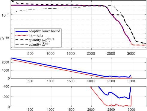
Figure 2: Matrix s3dkt3m2, top part: the $A$-norm of the error vector $x-x_{k}$ (dots), the square root of the upper bound $\omega_{d}^{\scriptscriptstyle(\mu)}$ (bold dashed), the quantity $\widetilde{\Delta}_{k}^{1/2}$ (dashed), and the lower bound with the adaptive choice of $d$ based on replacing $\varepsilon_{k+d+1}$ in (10) by $\widetilde{\Delta}_{k+d+1}$ (blue solid curve). Bottom parts: the adaptive value $d_{k}$ (blue bold solid curve) and the ideal value $\widetilde{d}_{k}$ (red solid curve).

This is clearly demonstrated in Figure 2, where the example s3dkt3m2 is considered. In the top part of the figure we plot the $A$-norm of $x-x_{k}$ (dotted curve), the quantity $\widetilde{\Delta}_{k}^{1/2}$ (dashed curve) defined using (21), and the square root of the Gauss–Radau upper bound $\omega_{k}^{\scriptscriptstyle(\mu)}$ defined in (20) (bold dashed curve). Note that to compute the upper bound $\omega_{k}^{\scriptscriptstyle(\mu)}$, we have to provide a tight underestimate $\mu$ of the smallest eigenvalue of the preconditioned matrix. For experimental reasons, we computed the smallest Ritz value at an iteration $k$ in which the ultimate level of accuracy was reached, and got a very accurate approximation to the smallest eigenvalue of the preconditioned matrix. Then we defined $\mu$ to be this computed approximation to the smallest eigenvalue divided by $1+10^{-4}$. We set $\tau=0.25$. If we use the quantity $\widetilde{\Delta}_{k+d+1}$ to approximate $\varepsilon_{k+d+1}$ in the ratio (10), and choose $d$ such that the approximated radio is less than $\tau$, we obtain very tight lower bounds (blue solid curve). However, in the final stage of convergence that is very important for stopping the iterations, such an adaptively chosen $d$ differs from the ideal $\widetilde{d}_{k}$ by about 200 (the bottom part). In other words, we compute about 200 iterations of P(CG) more than necessary to reach a given level of accuracy. Note that very similar results will be obtained when using the Gauss–Radau upper bound (20) to approximate $\varepsilon_{k+d+1}$ in the ratio (10), since normal and bold dashed curves almost coincide in the final stage of convergence. We will show how to fix these problems with the Gauss–Radau upper bound in a forthcoming paper.

In summary, the strategy for the adaptive choice of $d$ based on replacing $\varepsilon_{k+d+1}$ by $\widetilde{\Delta}_{k+d+1}$ or by $\omega_{k+d+1}^{\scriptscriptstyle(\mu)}$ in (10), seems to be a safe strategy in the sense that it usually produces $d$ larger than their ideal counterparts. For such $d$’s, the inequality (10) is satisfied. On the other hand, it can use values of $d$ that are significantly larger than necessary to reach the prescribed accuracy of the estimate $\Delta_{k:k+d}$. In particular, we observed unnecessarily large values of $d$ in the later (P)CG convergence phase. Therefore, it is better to use the strategy of Algorithm 2, eventually combined with the strategy for choosing the initial value of $d$.

6 Numerical experiments

In the following numerical experiments we consider a set of test problems from the SuiteSparse Matrix collection, listed in Table 1. We believe that the selected problems represent the most relevant scenarios one can face in practical computations. The experiments were run using double precision in MATLAB R2019b.

name	size	rhs $b$	precond. $M=LL^{T}$
bcsstk02	66	} 310em[ equal components]	—
bcsstk04	132		—
bcsstk09	1083		ict(1e-3, 1e-2)
s3dkt3m2	90 449	comes with the matrix	ict(1e-5, 1e-2)
s3dkq4m2	90 449	} 510em[ $\mbox{rand}(-1,1)$]	ict(1e-5, 1e-2)
pwtk	217 918		ict(1e-5, 1e-1)
af_shell3	504 855		zero-fill
tmt_sym	726 713		zero-fill
ldoor	952 203		zero-fill

Table 1: A set of test problems from the SuiteSparse Matrix collection.

When it is not provided with the matrix, the right-hand side $b$ is chosen such that $b$ has equal components in the eigenvector basis or such that the entries of $b$ are randomly generated in the interval $(-1,1)$. In both cases, $b$ is normalized to have the unit norm $\|b\|=1$. The right-hand side for s3dkt3m2 with only the last element nonzero comes with the application; see [13].

The preconditioners are determined by the incomplete Cholesky factorization (using the ichol command), either with zero-fill or with threshold dropping (ict) where the first parameter is the drop tolerance and the second parameter is the global diagonal shift; for more details see the MATLAB documentation.

In Figures 3 to 6 we test the accuracy of the lower bound $\Delta_{k:k+d_{k}}^{\scriptscriptstyle 1/2}$ as an approximation of the $A$-norm of the error vector $x-x_{k}$, $\|x-x_{k}\|_{A}=\varepsilon_{k}^{\scriptscriptstyle 1/2}$, where $d_{k}$ is determined as in Algorithm 2. In the top parts of Figures 3 to 6 we plot the lower bound $\Delta_{k:k+d_{k}}^{\scriptscriptstyle 1/2}$ (blue solid curve) together with $\|x-x_{k}\|_{A}$ (red dots). In the middle parts of figures we plot the relative error

$$\frac{\varepsilon_{k}-\Delta_{k:k+d_{k}}}{\varepsilon_{k}}$$

(blue solid curve) together with the prescribed tolerance $\tau=0.25$ (dotted line); see (7). Finally, in the bottom parts of Figures 3 to 6 we plot the value of $d_{k}$ determined by Algorithm 2, and compare it with the ideal value $\widetilde{d}_{k}$ of Definition 3.1. Note that the ideal value $\widetilde{d}_{k}$ was determined using the quantities $\varepsilon_{k}$ that are not known in practical computations.

bcsstk02

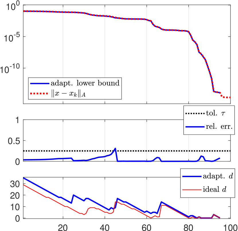
CG iterations

bcsstk04

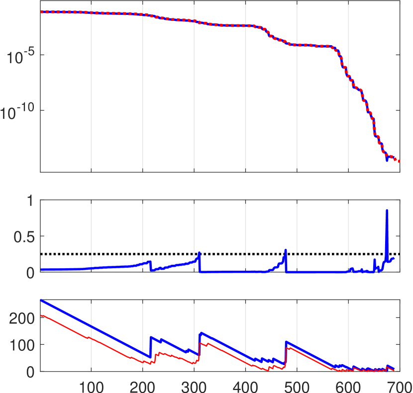
CG iterations

Figure 3: Matrices bcsstk02 and bcsstk04: the $A$-norm of the error vector $x-x_{k}$ and the adaptive lower bound (top part), the relative error and the prescribed tolerance from (7) (middle part), the value $d_{k}$ and the ideal value $\widetilde{d}_{k}$ (bottom part).

For the first two test problems (Figure 3), the unpreconditioned CG method needs significantly more iterations than what is the size of the problem to reach the ultimate level of accuracy. In other words, convergence is substantially delayed due to finite precision arithmetic. We choose these examples to demonstrate that the estimates and techniques for the adaptive choice of $d$ work well also in finite precision. This is actually no surprise. Using results of [21] we know that the estimation process is based on identities that do hold (up to some small inaccuracy) also during finite precision computations, despite the loss of orthogonality, until the ultimate level of accuracy is reached. One can observe that the required accuracy of estimates is reached and that the value of $d_{k}$ is close to the ideal value $\widetilde{d}_{k}$ in almost all iterations.

bcsstk09+no precond.

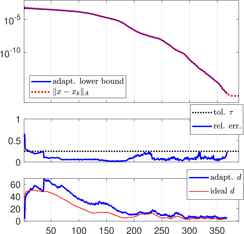
CG iterations

bcsstk09+ict(1e-3, 1e-2)

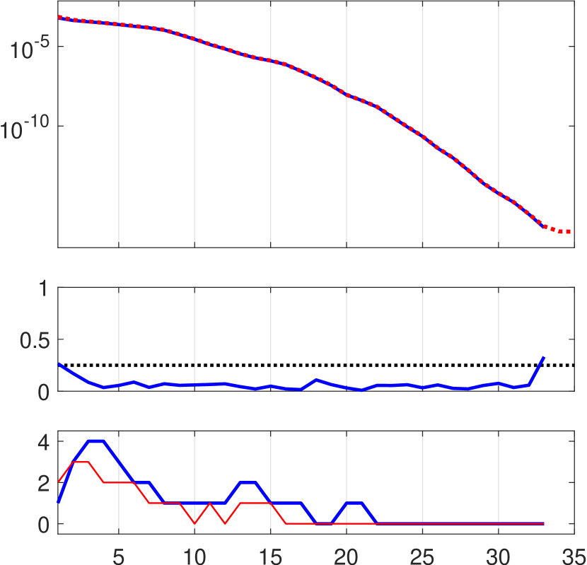
PCG iterations

Figure 4: Matrix bcsstk09 without and with the preconditioner: the $A$-norm of the error vector $x-x_{k}$ and the adaptive lower bound (top part), the relative error and the prescribed tolerance from (7) (middle part), the value $d_{k}$ and the ideal value $\widetilde{d}_{k}$ (bottom part).

In Figure 4 we test the performance of the adaptive procedure by considering the test problem bcsstk09 of size $1083$ with and without a preconditioner. Similarly as in the previous example, the adaptive strategy of Algorithm 2 works satisfactorily and provides estimates with the prescribed accuracy.

In the unpreconditioned case, the convergence is at first quite slow so that one needs larger values of $d_{k}$ (around 50) to reach the prescribed accuracy. As soon as convergence accelerates (around iteration 200), just a moderate value of $d_{k}$ (around 10) is needed. Our strategy perfectly captures this behavior, though in the beginning $d_{k}$ overestimates the ideal value $\widetilde{d}_{k}$ moderately. However, this should not represent a serious drawback in practical computations since the iterations will probably be stopped after iteration 200, when $d_{k}$ and the ideal $\widetilde{d}_{k}$ almost coincide. If stopped earlier, we just obtain a more accurate estimate than necessary.

In the preconditioned case, convergence is fast and the adaptive strategy provides values of $d_{k}$ that are almost identical to $\widetilde{d}_{k}$. This is in particular true in the final convergence phase when $\widetilde{d}_{k}=0$ so that PCG uses only terms from the current iteration. Hence, in this example, the adaptive strategy works very well in the case of fast convergence and no unnecessary iterations are needed.

pwtk

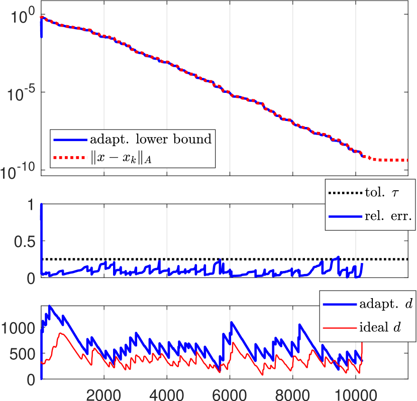
PCG iterations

af_shell3

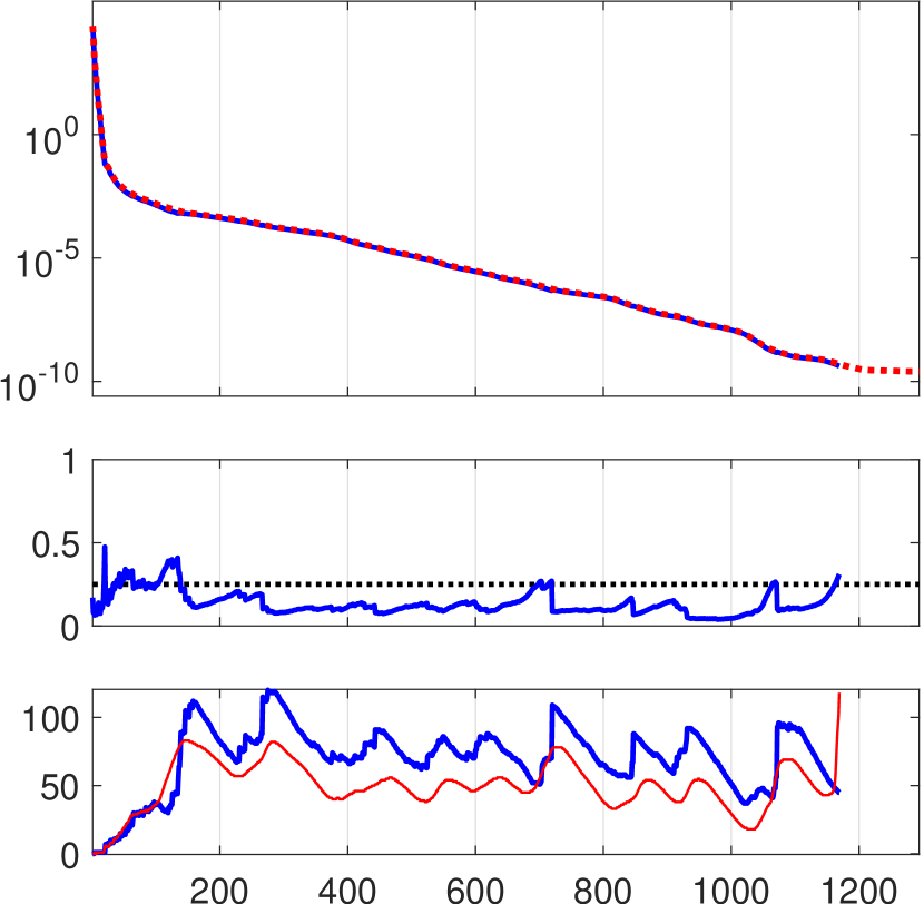
PCG iterations

tmt_sym

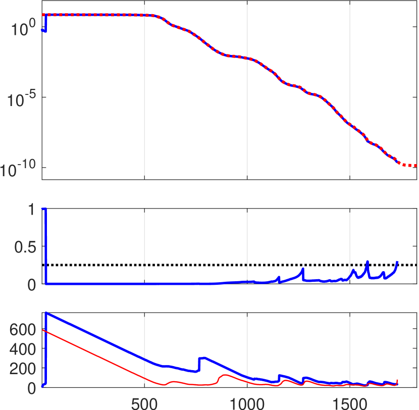
PCG iterations

ldoor

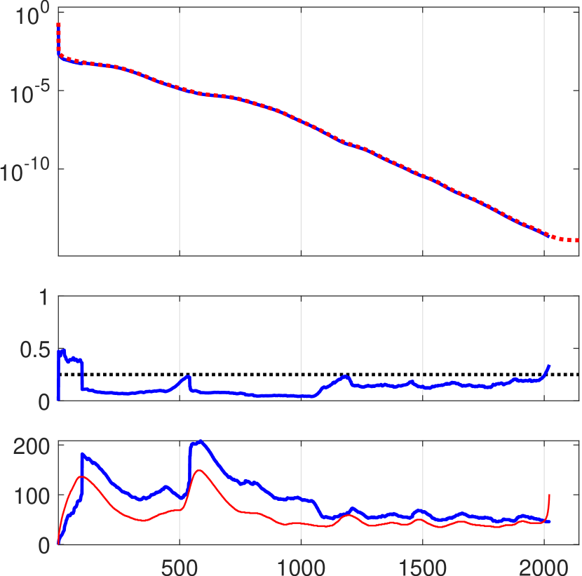
PCG iterations

Figure 5: Matrices pwtk, af_shell3, tmt_sym, ldoor: the $A$-norm of the error vector $x-x_{k}$ and the adaptive lower bound (top part), the relative error and the prescribed tolerance from (7) (middle part), the value $d_{k}$ and the ideal value $\widetilde{d}_{k}$ (bottom part).

In Figure 5 we consider quite large problems pwtk, af_shell3, tmt_sym, and ldoor that we are still able to handle using MATLAB on a personal computer. In all four cases, PCG was used to solve the systems. We can again conclude that our adaptive strategy works satisfactorily and provides tight bounds. Algorithm 2 can handle slow or fast convergence (as for pwtk and ldoor), the staircase convergence (pwtk and tmt_sym) and (mostly) also initial quasi-stagnation phases (tmt_sym). In some iterations, the value $d_{k}$ overestimates moderately the ideal value $\widetilde{d}_{k}$, providing more accurate adaptive estimates than required. On the other hand, it is better to slightly overestimate the ideal value of $\widetilde{d}_{k}$ than to underestimate it. As in the previous examples we observe that in iterations that are suitable for stopping the algorithm (a few orders of magnitude above the ultimate level of accuracy), the adaptively determined $d_{k}$ is very close to the ideal $\widetilde{d}_{k}$ so that no unnecessary iterations are needed to get the estimates with the required accuracy.

Note that in the test problem tmt_sym, the $A$-norm of the error vector exhibits quite a long initial quasi-stagnation phase (up to the iterations 500). In such cases, $d_{k}$ computed by Algorithm 2 need not be close to $\widetilde{d}_{k}$ in a few initial iterations. As a result, the lower bound $\Delta_{k:k+d_{k}}^{\scriptscriptstyle 1/2}$ can underestimate visibly the quantity of interest $\varepsilon_{k}^{\scriptscriptstyle 1/2}$; see also the test problem bcsstk04_sym (Figure 3). In such cases, the strategy for the initial choice of described in Section 5.1 should be used. This strategy will be discussed in more detail in a later experiment.

s3dkt3m2

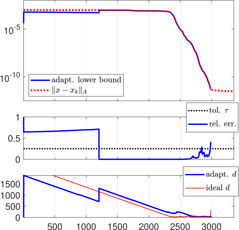
PCG iterations

s3dkq4m2

PCG iterations

Figure 6: Matrices s3dkt3m2, s3dkq4m2: the $A$-norm of the error vector $x-x_{k}$ and the adaptive lower bound (top part), the relative error and the prescribed tolerance from (7) (middle part), the value $d_{k}$ and the ideal value $\widetilde{d}_{k}$ (bottom part).

In Figure 6 we show the most difficult cases we have found when testing Algorithm 2 for the adaptive choice of $d_{k}$. In the test problems s3dkt3m2 and s3dkq4m2, the $A$-norm of the error vector exhibits various phases of the convergence (sublinear, superlinear, quasi-stagnation) that alternate. The quasi-stagnation phase can happen at the very beginning as for s3dkt3m2 but also in later iterations as for s3dkq4m2. Such a complicated convergence behaviour need not be fully captured by Algorithm 2. At some iterations, the resulting $d_{k}$ underestimates significantly the ideal value $\widetilde{d}_{k}$ and, therefore, we observe visually a considerable underestimation of the quantity of interest. While for s3dkt3m2 we are able to fix the problem using a suitable initial $d_{0}$, see Section 5.1 and Figure 8, for the problem s3dkq4m2 we were not able to find an improvement that would prevent an underestimation close to the iteration 1000.

Nevertheless, though the strategy of Algorithm 2 applied to the test problems shown in Figure 6 does not always provide estimates of $\|x-x_{k}\|_{A}$ with a required accuracy, it can still be considered as satisfactory. It provides lower bounds that are close to the quantity of interest (they are of the same magnitude) so that one could use them in stopping criteria. Moreover, in both cases, $d_{k}$ is very close to $\widetilde{d}_{k}$ in the final convergence phase that is suitable for stopping the algorithm.

In Figure 7 we demonstrate the technique of Section 5.1 for the initial choice of $d_{0}$. As already observed in test problems bcsttk04, tmt_sym, and s3dkt3m2, Algorithm 2 can provide smaller values of $d_{k}$ than needed in the initial quasi-stagnation phase. One can overcome this trouble by the strategy presented in Section 5.1 when approximating the nominator in (22) using the quantity (21) that does not need any a priory information or using the Gauss–Radau upper bound, if available. In our experiment we use Algorithm 4, i.e., the quantity (21).

For both test problems tmt_sym and s3dkt3m2, the strategy based on the criterion (22) determines properly a safe value $d_{0}$ that ensures the prescribed relative accuracy of the initial estimate. The value $d_{0}$ overestimates the ideal value $\widetilde{d}_{0}$ which means that the error has significantly decreased in $d_{0}$ iterations of PCG, and that the initial estimate is more accurate than required. In other words, using $d_{0}$ we have safely overcame the initial quasi-stagnation phase.

After $d_{0}$ is found in Algorithm 4, we continue along the lines of Algorithm 2. In particular, we immediately get the estimates of the $A$-norm of the error vector for the initial plateau since the values of $k$ are increased and the values of $d$ are decreased on line 12 of Algorithm 2, without computing further PCG iterations. Once the criterion (12) is not met, we continue to use the standard strategy of Algorithm 2. Again, $d_{k}$ is very close to $\widetilde{d}_{k}$ in the final convergence phase.

s3dkt3m2+$d_{0}$

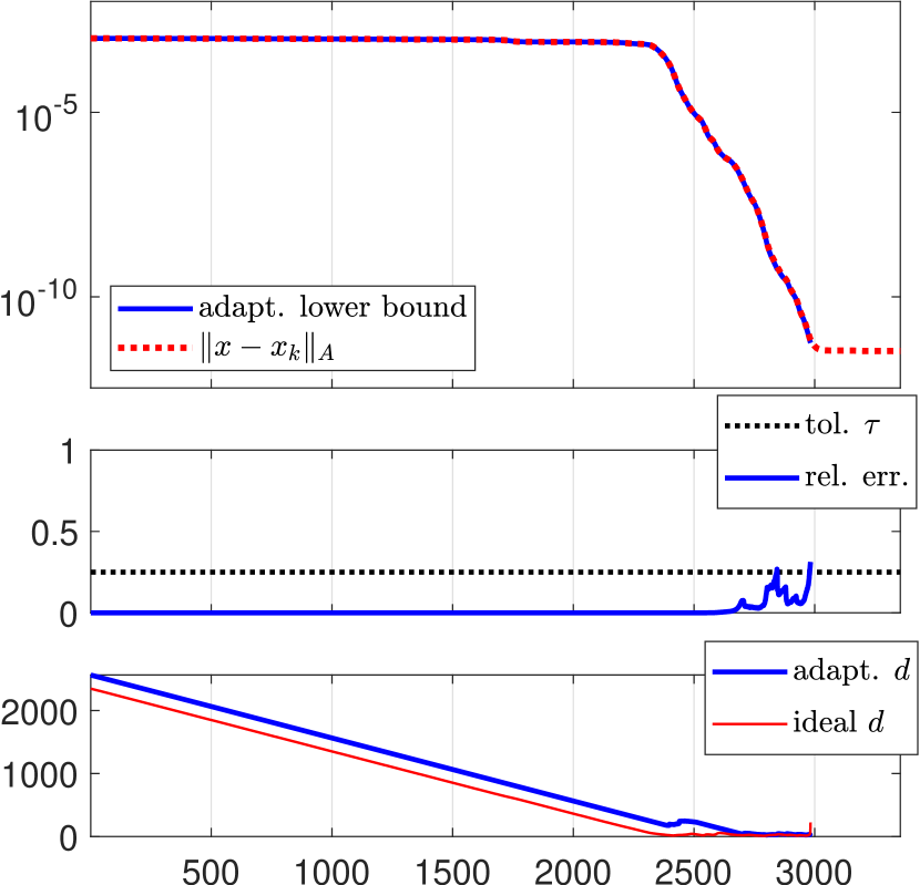
PCG iterations

tmt_sym+$d_{0}$

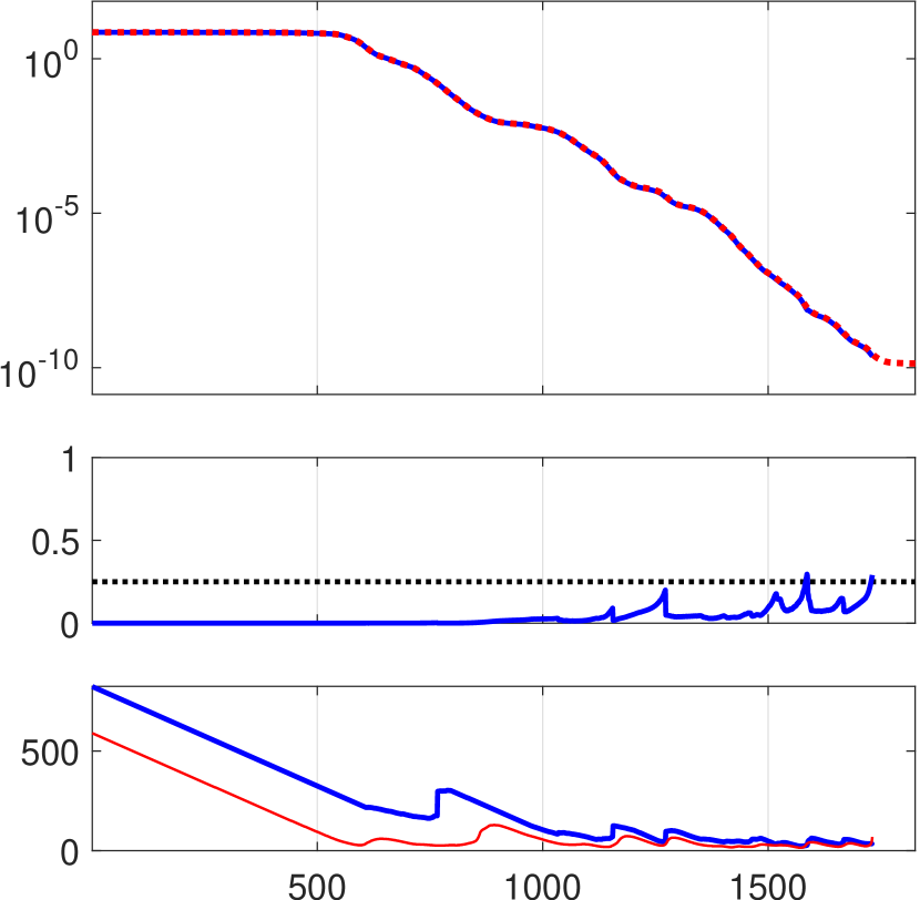
PCG iterations

Figure 7: Matrices s3dkt3m2 and tmt_sym with the adaptive algorithm of Section 5.1 to determine the initial value $d_{0}$: the $A$-norm of the error vector $x-x_{k}$ and the adaptive lower bound (top part), the relative error and the prescribed tolerance from (7) (middle part), the value $d_{k}$ and the ideal value $\widetilde{d}_{k}$ (bottom part).

bcsstk04

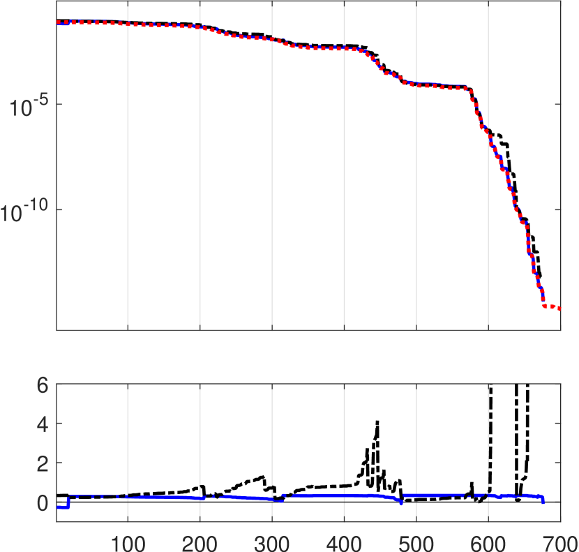
PCG iterations

s3dkt3m2

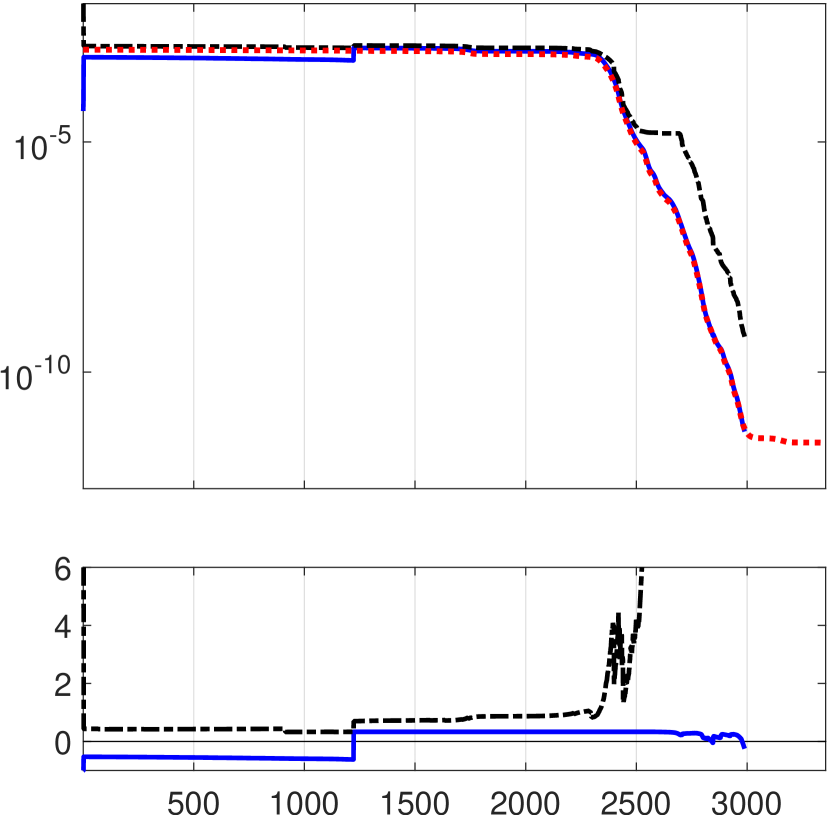
PCG iterations

Figure 8: Matrices bcsstk04 and s3dkt3m2. Top part: the $A$-norm of the error vector $x-x_{k}$ (red dashed curve), the square root of the heuristic upper bound (8) (blue solid curve), and the square root of the upper bound (24) (black dash-dotted curve). Bottom part: the accuracy of bounds measured by the relative quantities (25).

Finally, in the last Figure 8 we test the quality of the heuristic upper bound (8),

(23) $$\frac{\Delta_{k:k+d}}{1-\tau}$$

that uses the adaptive choice of $d_{k}$ as in Algorithm 2. We know that if $d_{k}$ is chosen such that (7) is satisfied (if $d_{k}\geq\widetilde{d}_{k}$), then (23) represents an upper bound on $\varepsilon_{k}$. Note that even though the heuristic upper bound (23) is not guaranteed to be an upper bound in general, its advantage is that no estimates of eigenvalues are needed. We compare the heuristic upper bound (23) with the upper bound $\Omega_{k:k+d}^{\scriptscriptstyle(\mu)}$ defined below that uses the same number of $d_{k}$ terms as the quantity (23). In particular, the bound $\Omega_{k:k+d}^{\scriptscriptstyle(\mu)}$ is defined using the identity (5) with the last term $\varepsilon_{k+d}$, and the Gauss–Radau upper bound (20) on $\varepsilon_{k+d}$,

(24) $$\|x-x_{k}\|^{2}_{A}\leq\Delta_{k:k+d-1}+\alpha_{k+d}^{\scriptscriptstyle(\mu)}\|r_{k+d}\|^{2}\equiv\Omega_{k:k+d}^{\scriptscriptstyle(\mu)}.$$

The bound (24) depends on an a priori given underestimate $\mu$ to the smallest eigenvalue of the (preconditioned) system matrix. In our experiments, the underestimate $\mu$ was computed in the same way as described in Section 5.2.

In the top part of Figure 8 we plot $\|x-x_{k}\|_{A}$ (red dots) together with the upper bound $(\Omega_{k:k+d_{k}}^{\scriptscriptstyle(\mu)})^{1/2}$ and the heuristic upper bound given by the square root of (23); in the bottom part, we check the quality of bounds using the relative quantities

(25) $$\frac{\Omega_{k:k+d_{k}}^{\scriptscriptstyle(\mu)}-\varepsilon_{k}}{\varepsilon_{k}}\ \mbox{(dashed)}\quad\mbox{ and }\quad\frac{\frac{\Delta_{k:k+d_{k}}}{1-\tau}-\varepsilon_{k}}{\varepsilon_{k}}\ \mbox{(solid)}.$$

Obviously, the considered heuristic upper bound is more accurate than the Gauss–Radau upper bound in the convergence phase that is crucial for stopping the iterations. In a future work we would like to explain the behavior of the Gauss–Radau upper bound (why it is delayed) and possibly fix the problem seen in the last iterations.

7 Summary and concluding discussion

In this paper we focused on the accurate estimation of the error $\varepsilon_{k}$ in the P(CG) method. Our approach is based on the Hestenes and Stiefel formula (5) that is well preserved also during finite precision computations. Our goal was to find a nonnegative integer $d$ (ideally the smallest one) such that the relative accuracy of the estimate $\Delta_{k:k+d}$ is less than or equal to a prescribed tolerance $\tau$. The developed technique for the adaptive choice of $d$ is purely heuristic so that the accuracy of the estimate $\Delta_{k:k+d}$ cannot be guaranteed in general. Nevertheless, the heuristic strategy has shown to be robust and reliable, which was demonstrated by numerical experiments. Moreover, in the final stage of convergence that is suitable for stopping the iterations, the suggested value of $d$ is usually very close to the optimal (ideal) one so that one avoids unnecessary iterations.

One can also think of many other different adaptive strategies that are based, e.g., on the Gauss–Radau or anti-Gaussian quadrature rules, or on other techniques for approximating the ratio (10). We have tested many of them, and the strategy suggested in this paper seems to be efficient, simple, and robust.

Our techniques can also be adjusted for estimating the relative quantities

$$\frac{\|x-x_{k}\|_{A}^{2}}{\|x-x_{0}\|^{2}_{A}}\quad\mbox{or}\quad\frac{\|x-x_{k}\|_{A}^{2}}{\|x\|^{2}_{A}}$$

using the fact that $\|x\|_{A}^{2}=\|x-x_{0}\|^{2}_{A}+b^{T}x_{0}+r_{0}^{T}x_{0}$; see also [22].

We hope that the results presented in this paper will prove to be useful in practical computations. They allow to approximate the error $\varepsilon_{k}$ at a negligible cost during (P)CG iterations without any user-defined parameter, while taking into account the prescribed relative accuracy of the estimate.

Appendix A Algorithm 2 (MATLAB code, preconditioned version)

⬇

1function [x,estim,delay] = pcga(A,b,tau,maxit,L,x)

2%% ... preconditioned CG with the adaptive choice of d

3

4r = b - A * x; % ... pcg initialization

5z = L\r; z = L’\z; p = z;

6rr = z’ * r;

7k = 1; d = 0;

8

9for ell = 1:maxit+1

10

11 RR = rr; % ... begin cgiter(ell)

12 Ap = A * p;

13 alpha = RR/(p’ * Ap);

14 x = x + alpha * p;

15 r = r - alpha * Ap;

16 z = L \ r; z = L’ \ z;

17 rr = z’ * r;

18 beta = rr / RR;

19 p = z + beta * p; % ... end cgiter(ell)

20

21 Delta(ell) = alpha * RR;

22 curve(ell) = 0;

23 curve = curve + Delta(ell);

24

25 if ell > 1 % ... adaptive choice of d

26 S = findS(curve,Delta,k);

27

28 num = S * Delta(ell);

29 den = sum(Delta(k:ell-1));

30

31 while (d >= 0) && (num/den <= tau)

32 delay(k) = d;

33 estim(k) = den;

34 k = k + 1; d = d - 1;

35 den = sum(Delta(k:ell-1));

36 end

37 d = d + 1;

38 % ... use estim(k-1) in stopping criteria, if k > 1

39 end

40end

41end % of function

42

43function [S] = findS(curve,Delta,k)

44%% ... find the safety factor S using the tolerance 1e-4

45

46ind = find((curve(k)./curve) <= 1e-4, 1, ’last’);

47if isempty(ind), ind = 1; end

48

49S = max(curve(ind:end-1)./Delta(ind:end-1));

50end

References

- [1] M. Arioli, A stopping criterion for the conjugate gradient algorithms in a finite element method framework, Numer. Math., 97 (2004), pp. 1–24.
- [2] M. Arioli, E. H. Georgoulis, and D. Loghin, Stopping criteria for adaptive finite element solvers, SIAM J. Sci. Comput., 35 (2013), pp. A1537–A1559.
- [3] V. Dolejší and P. Tichý, On efficient numerical solution of linear algebraic systems arising in goal-oriented error estimates, J. Sci. Comput., 83 (2020), pp. 1–29.
- [4] T. Gergelits, K.-A. Mardal, B. F. Nielsen, and Z. Strakoš, Laplacian preconditioning of elliptic PDEs: localization of the eigenvalues of the discretized operator, SIAM J. Numer. Anal., 57 (2019), pp. 1369–1394.
- [5] T. Gergelits, B. F. Nielsen, and Z. Strakoš, Generalized spectrum of second order differential operators, SIAM J. Numer. Anal., 58 (2020), pp. 2193–2211.
- [6] G. H. Golub and G. Meurant, Matrices, moments and quadrature, in Numerical analysis 1993 (Dundee, 1993), vol. 303 of Pitman Res. Notes Math. Ser., Longman Sci. Tech., Harlow, 1994, pp. 105–156.
- [7] G. H. Golub and G. Meurant, Matrices, moments and quadrature. II. How to compute the norm of the error in iterative methods, BIT, 37 (1997), pp. 687–705.
- [8] G. H. Golub and Z. Strakoš, Estimates in quadratic formulas, Numer. Algorithms, 8 (1994), pp. 241–268.
- [9] A. Greenbaum, Behavior of slightly perturbed Lanczos and conjugate-gradient recurrences, Linear Algebra Appl., 113 (1989), pp. 7–63.
- [10] A. Greenbaum and Z. Strakoš, Predicting the behavior of finite precision Lanczos and conjugate gradient computations, SIAM J. Matrix Anal. Appl., 13 (1992), pp. 121–137.
- [11] M. R. Hestenes and E. Stiefel, Methods of conjugate gradients for solving linear systems, J. Research Nat. Bur. Standards, 49 (1952), pp. 409–436.
- [12] P. Jiránek, Z. Strakoš, and M. Vohralík, A posteriori error estimates including algebraic error and stopping criteria for iterative solvers, SIAM J. Sci. Comput., 32 (2010), pp. 1567–1590.
- [13] R. Kouhia, Description of the CYLSHELL set, tech. report, Aalto University, May 1998. Matrix Market.
- [14] M. Kubínová and I. Pultarová, Block preconditioning of stochastic Galerkin problems: new two-sided guaranteed spectral bounds, SIAM/ASA J. Uncertain. Quantif., 8 (2020), pp. 88–113.
- [15] G. Meurant, Numerical experiments in computing bounds for the norm of the error in the preconditioned conjugate gradient algorithm, Numer. Algorithms, 22 (1999), pp. 353–365.
- [16] G. Meurant, The Lanczos and conjugate gradient algorithms: From Theory to Finite Precision Computations, vol. 19 of Software, Environments, and Tools, Society for Industrial and Applied Mathematics (SIAM), Philadelphia, PA, 2006.
- [17] G. Meurant and Z. Strakoš, The Lanczos and conjugate gradient algorithms in finite precision arithmetic, Acta Numer., 15 (2006), pp. 471–542.
- [18] G. Meurant and P. Tichý, On computing quadrature-based bounds for the -norm of the error in conjugate gradients, Numer. Algorithms, 62 (2013), pp. 163–191.
- [19] G. Meurant and P. Tichý, Approximating the extreme Ritz values and upper bounds for the -norm of the error in CG, Numer. Algorithms, 82 (2019), pp. 937–968.
- [20] C. C. Paige, Accuracy and effectiveness of the Lanczos algorithm for the symmetric eigenproblem, Linear Algebra Appl., 34 (1980), pp. 235–258.
- [21] Z. Strakoš and P. Tichý, On error estimation in the conjugate gradient method and why it works in finite precision computations, Electron. Trans. Numer. Anal., 13 (2002), pp. 56–80.
- [22] Z. Strakoš and P. Tichý, Error estimation in preconditioned conjugate gradients, BIT, 45 (2005), pp. 789–817.