Machine Learning for Vibrational Spectroscopy via Divide-and-Conquer Semiclassical Initial Value Representation Molecular Dynamics with Application to N-Methylacetamide

Abstract

A machine learning algorithm for partitioning the nuclear vibrational space into subspaces is introduced. The subdivision criterion is based on Liouville’s theorem, i.e. best preservation of the unitary of the reduced dimensionality Jacobian determinant within each subspace along a probe full-dimensional classical trajectory. The algorithm is based on the idea of evolutionary selection and it is implemented through a probability graph representation of the vibrational space partitioning. We interface this customized version of genetic algorithms with our divide-and-conquer semiclassical initial value representation method for calculation of molecular power spectra. First, we benchmark the algorithm by calculating the vibrational power spectra of two model systems, for which the exact subspace division is known. Then, we apply it to the calculation of the power spectrum of methane. Exact calculations and full-dimensional semiclassical spectra of this small molecule are available and provide an additional test of the accuracy of the new approach. Finally, the algorithm is applied to the divide-and-conquer semiclassical calculation of the power spectrum of 12-atom trans-N-Methylacetamide.

I Introduction

When full-dimensional calculations are not computationally feasible, one needs to introduce some sort of approximation. This happens quite often in quantum molecular dynamics because the full-dimensional potential V(q) is generally non separable. However, if the system potential were made of the sum of a finite number of lower dimensional terms of the type $V_{a}\left(q_{1},\>q_{2}\right)+V_{b}\left(q_{\text{3}}\right)+V_{c}\left(q_{4},\>q_{5},\>q_{6}\right)+...$, then each collection of variables within the several terms would compose a sensible subspace suitable for an independent calculation. Unfortunately, this is not the case for nuclear dynamics, but one may wonder which is the decomposition of the full-dimensional vibrational space into subspaces such that the couplings between different subspace modes are minimized. The main goal of this paper is to provide a possible answer to this issue by means of a clustering optimization algorithm.

The algorithm we propose has its roots in the sound ground of Genetic Algorithms (GAs), but it is different for technical definitions and implementation and we will refer to it with the more general label of Evolutionary Algorithm. The theoretical background and implementation of GAs could be traced back to the works of Holland, Goldberg, and Henry.Holland (1962); Goldberg and Holland (1988); Holland et al. (1992) Since then, they have been successfully applied to various problems in analytical chemistry and chemometrics, such as the analysis of NMR pulse patterns from complex molecules,Freeman and Xili (1987) the optimal choice of wavelengths to determine the concentration of a sample, and conformational analysis. Hibbert (1993) GAs have been proven to be the first choice in many cases of feature selection in regression and classification problems in general Leardi (2001); Niazi and Leardi (2012) and in Quantitative Structure Activity Relationships in particular.Beheshti et al. (2016); Niazi and Leardi (2012) Evolutionary Algorithms have also been used in materials science to study the dynamical properties of molecules on surfaces during molecular dynamics simulations.Bhattacharya et al. (2009)

We test the accuracy of the new optimization algorithm when applied to the calculation of vibrational power spectra using semiclassical molecular dynamics. Specifically, we employ the divide-and-conquer approach to the time-averaged semiclassical initial value representation (DC-SCIVR) method for nuclear power spectrum calculations.Ceotto, Di Liberto, and Conte (2017) In the DC-SCIVR strategy, the vibrational space is divided into subspaces to overcome the issue of the full-dimensional calculation. So far, at the best of our knowledge, three methods for the partition of the full-dimensional vibrational problem into lower dimensional subspaces have been proposed. These are the Hessian method,Di Liberto, Conte, and Ceotto (2018a) the Wehrle-Šulc-Vaníc̆ek method,Wehrle, Sulc, and Vanicek (2014) and the Jacobi method.Di Liberto, Conte, and Ceotto (2018a) According to the latter, the residual coupling between subspaces is estimated by recurring to Liouville’s theorem. In few words, the best clustering of vibrational modes is the one where each subspace preserves as much as possible its phase space volume during a classical, full-dimensional trajectory. This approach has the advantage of being based on dynamics, i.e. it depends on both nuclear kinetic and potential contributions. Originally, we applied this method by searching over all possible subspace combinations. As a matter of fact, the problem scales approximately as a binomial factor times the number of subspaces $n_{s}$, i.e. $\sim n_{s}\times F!/D!(F-D)!$, where $F$ is the number of degrees of freedom and $D$ is the size of a subspace. Furthermore, it is not possible to know in advance how many subspaces one should choose and the size of each one.

In this work we introduce an Evolutionary Algorithm and another simplified and less demanding approach. Both are able to automatize these choices and highly reduce the computational cost of the optimization. The paper is organized as follows: In Sec. II, we recap the DC-SCIVR method and present the optimization algorithms. Sec. III presents our results for spectroscopic calculations and Sec. IV concludes the paper and offers some perspectives.

II Methods

II.1 Semiclassical spectra

The semiclassical power spectrum $I(E)$ of a system described by the Hamiltonian $\hat{H}$ is equal to the Fourier-transformed wavepacket survival amplitude (in atomic units)Heller (1981a)

$$I(E)=\frac{1}{2\pi}\intop_{-\infty}^{+\infty}e^{iEt}\langle\chi|\chi(t)\rangle dt,$$ (1)

where $|\chi\left(t\right)\rangle=e^{-i\hat{H}t}|\chi\rangle$ is the quantum time-evolution of the arbitrary reference state $|\chi\rangle$. By writing the reference state as a linear combination of the Hamiltonian eigenstates $|\psi_{j}\rangle$, i.e. $|\chi\rangle=\sum_{j}c_{j}|\psi_{j}\rangle$, it can be shown that

$$I(E)=\sum_{j}|c_{j}|^{2}\delta(E-E_{j}).$$ (2)

Hence, the power spectrum is equal to a sum of delta functions centered at the vibrational frequencies $E_{j}$. A convenient way to calculate the formula in Eq. (1) is given by the time-averaging semiclassical initial value representation (TA-SCIVR) method.Kaledin and Miller (2003a, b); Miller (1968, 1971, 1998, 2001, 2005); Sun, Wang, and Miller (1998); Thoss, Wang, and Miller (2001); Yamamoto and Miller (2003) This is obtained by applying a time-averaging filter to the Heller-Herman-Kluk-Kay (HHKK) propagatorHeller (1981b); Herman and Kluk (1984); Miller (2002); Kluk, Herman, and Davis (1986); Kay (1994a, b, c, 2006); Grossmann and Xavier (1998); Antipov, Ye, and Ananth (2015); Church, Antipov, and Ananth (2017); Church and Ananth (2019); Buchholz et al. (2018), which defines the approximate quantum time evolution. The final TA-SCIVR expression of Eq. (1) for a system characterized by $F$ degrees of freedom reads

$$I(E)= \left(\frac{1}{2\pi}\right)^{F}\iint d\mathbf{p}_{0}d\mathbf{q}_{0}\>\frac{1}{2\pi T}$$ (3)

$$\bigg{|}\intop_{0}^{T}dt\,\langle\chi|\mathbf{p}_{t}\mathbf{q}_{t}\rangle e^{i\left(S_{t}(\mathbf{p}_{0},\mathbf{q}_{0})+\phi_{t}(\mathbf{p}_{0},\mathbf{q}_{0})+Et\right)}\bigg{|}^{2},$$

where $T$ is the total simulation time, $S_{t}(\mathbf{p}_{0},\mathbf{q}_{0})$ the instantaneous action of the classically evolved trajectory $\left(\mathbf{p}_{t},\mathbf{q}_{t}\right)$, and the phase-space integration is performed on the initial trajectory momenta $\mathbf{p}_{0}$ and positions $\mathbf{q}_{0}$. In the previous equation $|\mathbf{p}_{t}\mathbf{q}_{t}\rangle$ are coherent states with the following form in position representationHeller (1991)

$$\langle\mathbf{x}|\mathbf{p}_{t}\mathbf{q}_{t}\rangle= \left(\frac{\det(\bm{\gamma})}{\pi^{F}}\right)^{\frac{1}{4}}$$ (4)

$$\exp\left[-\frac{1}{2}\left(\mathbf{x}-\mathbf{q}_{t}\right)^{\mathrm{T}}\bm{\gamma}\left(\mathbf{x}-\mathbf{q}_{t}\right)+i\mathbf{p}_{t}^{\mathrm{T}}\left(\mathbf{x}-\mathbf{q}_{t}\right)\right],$$

where $\bm{\gamma}$ is an $F\times F$ diagonal matrix, whose elements are chosen to be numerically equal to the harmonic frequencies of the system. In Eq. (3), $\phi_{t}(\mathbf{p}_{0},\mathbf{q}_{0})$ is the phase of the HHKK prefactorDi Liberto and Ceotto (2016)

$$\phi_{t}(\mathbf{p}_{0},\mathbf{q}_{0})=$$

$$phase\left[\sqrt{\frac{1}{2^{F}}\left|\mathbf{M_{qq}}+\bm{\gamma}^{-1}\mathbf{M_{pp}}\bm{\gamma}-i\mathbf{M_{qp}}\bm{\gamma}+i\bm{\gamma}^{-1}\mathbf{M_{pq}}\right|}\right],$$ (5)

where $\mathbf{M_{ij}}$ with $\mathbf{i,j}=\mathbf{p},\mathbf{q}$ are the elements of the Jacobian (monodromy) matrix

$$\mathbf{J}=\begin{pmatrix}\mathbf{M_{pp}}&\mathbf{M_{pq}}\\ \mathbf{M_{qp}}&\mathbf{M_{qq}}\end{pmatrix}=\begin{pmatrix}\dfrac{\partial\mathbf{p}_{t}}{\partial\mathbf{p}_{0}}&\dfrac{\partial\mathbf{p}_{t}}{\partial\mathbf{q}_{0}}\\ \\ \dfrac{\partial\mathbf{q}_{t}}{\partial\mathbf{p}_{0}}&\dfrac{\partial\mathbf{q}_{t}}{\partial\mathbf{q}_{0}}\end{pmatrix}.$$ (6)

The determinant $\left|\det(\mathbf{J})\right|$ is always equal to 1 along the trajectory, in accordance with Liouville’s theorem. The major problem associated to the TA-SCIVR spectral density calculation is represented by the computational cost of the Monte Carlo phase-space integration in Eq. (3).Ma et al. (2018) To overcome this problem, the multiple coherent states SCIVR (MC SCIVR) has been introduced. The method relies on the idea that the most important contribution to the spectrum comes from the trajectories whose energies are as close as possible to the quantum mechanical eigenvalues.De Leon and Heller (1983) Thus, in MC SCIVR, the phase-space integral of Eq. (3) is formally replaced by a sum over the most relevant trajectories, i.e. those corresponding to the spectral signals of interest. The MC-SCIVR initial conditions for the $j$-th degree of freedom areCeotto et al. (2009a, b)

$$\begin{cases}q_{0}^{(j)}=q_{eq}^{(j)}\\ p_{0}^{(j)}=\sqrt{(2n_{j}+1)\omega_{j}}\end{cases},$$ (7)

being $q_{eq}^{(j)}$ the equilibrium position of the $j$-th mode, and $\omega_{j}$ its harmonic frequency. Our reference states are combinations of coherent states of the type

$$|\chi\rangle=\prod_{j}^{F}\left(|p_{0}^{(j)},q_{0}^{(j)}\rangle+\epsilon_{j}|-p_{0}^{(j)},q_{0}^{(j)}\rangle\right),$$ (8)

where $\epsilon_{j}=\pm 1$ according to which spectroscopic signal one wants to enhance. For example, a collection of +1 values allows one to enhance the ZPE signal (together with the even transitions), while a selected $\epsilon_{j}=-1$ and the remaining $\epsilon_{i\neq j}=+1$ enhances the odd transition of the $j-th$ mode.Ceotto, Tantardini, and Aspuru-Guzik (2011) MC SCIVR has been successfully applied to the study of several systems,Gabas, Conte, and Ceotto (2017); Ceotto, Dell‘ Angelo, and Tantardini (2010); Conte, Aspuru-Guzik, and Ceotto (2013); Micciarelli et al. (2019, 2018); Tamascelli et al. (2014); Buchholz, Grossmann, and Ceotto (2016, 2017, 2018); Zhuang et al. (2012); Ceotto, Zhuang, and Hase (2013); Aieta et al. (2020) including the different conformers of the glycine amino acid.Gabas, Conte, and Ceotto (2017) To improve with respect to the harmonic initial conditions of Eq.s (7), a preliminary adiabatic switching warm up can be implemented with the result that frequency estimates are generally more accurate and complications due to deterministic chaos are largely avoided.Conte et al. (2019)

However, for very high-dimensional systems, the overlap between the initial and the evolved wavepacket of Eq. (1) is smaller and smaller as the dimensionality increases, given that the reference states are the direct product of monodimensional coherent states. To overcome this limitation, the Divide-and-Conquer (DC) SCIVR method has been recently introduced. Ceotto, Di Liberto, and Conte (2017); Di Liberto, Conte, and Ceotto (2018a) The DC basic idea is to project the system onto lower-dimensional subspaces. Within these subspaces, it is possible to calculate reduced-dimensionality spectra. Then, the full-dimensional spectrum can be obtained by convolving the subdimensional ones. The DC-SCIVR working equation is

$$\tilde{I}(E)=\left(\frac{1}{2\pi}\right)^{D}\iint d\tilde{\mathbf{p}}_{0}d\tilde{\mathbf{q}}_{0}\>\frac{1}{2\pi T}\bigg{|}\intop_{0}^{T}dt\,\langle\tilde{\chi}|\tilde{\mathbf{p}}_{t}\tilde{\mathbf{q}}_{t}\rangle e^{i\left(\tilde{S}_{t}(\tilde{\mathbf{p}}_{0},\tilde{\mathbf{q}}_{0})+\tilde{\phi}_{t}(\tilde{\mathbf{p}}_{0},\tilde{\mathbf{q}}_{0})+Et\right)}\bigg{|}^{2},$$ (9)

where the quantities projected onto a $D$-dimensional subspace have been indicated with the tilde symbol. The DC-SCIVR approach has been successfully applied to complex and fluxional systems, like small water clustersDi Liberto, Conte, and Ceotto (2018b) and the protonated water dimer.Bertaina, Di Liberto, and Ceotto (2019) It is also possible to implement the multiple coherent states idea into the DC-SCIVR method by replacing the double integral of Eq. (9) with a sum running on the most relevant trajectories. This method, named MC-DC SCIVR, can deal with very high-dimensional systems. Notable applications of MC-DC SCIVR include dipeptide derivatives,Gabas et al. (2018) nucleobasesGabas, Di Liberto, and Ceotto (2019) and nucleosides, Gabas, Conte, and Ceotto (2020) and molecules adsorbed on titania surfaces.Cazzaniga et al. (2020) The most relevant issue to deal with for a successful DC-SCIVR calculation is the choice of the optimal subspace decomposition. In fact, all the quantities appearing in Eq. (9) can be exactly projected onto subspaces, except for the action, because the potential is not in general separable and its coupling terms significantly change the action. To project the action, we adopted the following equation

$$\tilde{S}_{t}(\tilde{\mathbf{p}}_{0},\tilde{\mathbf{q}}_{0})=\intop_{0}^{t}dt^{\prime}$$

$$\left[\frac{1}{2}\,\tilde{\mathbf{p}}_{t^{\prime}}^{T}\tilde{\mathbf{p}}_{t^{\prime}}-\left(V(\tilde{\mathbf{q}}_{t^{\prime}},\mathbf{q}_{t^{\prime}}^{(F-D)})-V(\tilde{\mathbf{q}}_{eq},\bm{q}_{t^{\prime}}^{(F-D)})\right)\right],$$ (10)

which is exact for separable potentials.Ceotto, Di Liberto, and Conte (2017) The projected pre-exponential factor is obtained by substituting the elements of the $2M\times 2M$ sub-block Jacobian matrix of the type of Eq. (6) into the prefactor equation (5).

Between the possible criteria that one can adopt to partition the vibrational space into subspaces, the one that makes each $2D\times 2D$ sub-block Jacobian matrix determinant closer to 1 is the less severe approximation for the reduced dimensionality spectra. We have called this procedure the “Jacobi method”.Di Liberto, Conte, and Ceotto (2018a) By recalling Liouville’s theorem, this vibrational space subdivision is the one that minimizes the energy exchange between subspaces, because an ideal partition where each sub-block determinant is equal to unity preserves the energy within each subspace. More specifically, we compute the Jacobian matrix (Eq. (6)), which, in turn, is computed during the dynamics according to the prescription given by Brewer et al. Brewer, Hulme, and Manolopoulos (1997).

The main goal of this work is to find an efficient method for the subdivision of the Jacobian matrix of Eq. (6) into a number $n_{s}$ of subdimensional Jacobian matrices, each containing a cluster of normal modes, such that each subspace evolution $\left(\tilde{\mathbf{p}}_{t},\tilde{\mathbf{q}}_{t}\right)$ is the closest possible to satisfy Liouville’s theorem. In other words, an optimal choice of the normal mode clustering would lead to $\prod_{i}^{n_{s}}\det\mathbf{\tilde{J}}_{i}$ as close as possible to 1, where $\tilde{\mathbf{J}}_{i}$ is the Jacobian matrix of subspace $i$, and it is extracted from the full-dimensional Jacobian simply selecting all the entries involving the modes that belong to subspace $i$. In our procedure, we compute the Jacobian matrix at every time step along a test trajectory, which starts from the equilibrium position of the atom coordinates and with initial kinetic energy equal to the harmonic zero point energy. Originally,Di Liberto, Conte, and Ceotto (2018a) we presented a hierarchical search of the most frequently selected subspaces along the test trajectory in a two-step procedure. First, for each possible dimensionality $1\dots D<F$, all the ${F\choose D}$ possible subspaces were considered and the most frequently chosen along the dynamics were saved. Then, the absolute value of the deviation from 1 of each subspace Jacobian was computed at each time step, and the optimal subspace for each dimensionality was declared the one with the smallest average deviation. The subspace associated with the overall smallest deviation was selected and the whole procedure reiterated on the remaining degrees of freedom until all modes had been included into a subspace. This approach has still a non convenient computational scaling cost which is proportional to $\sum_{D=1}^{F-1}D\binom{F}{D}$, since all subspace combinations need to be tested. Furthermore, it is hierarchical and thus prone to find local optima for the global subdivision. In this study, we develop and test an algorithm able to find the global optimal subspaces with lower computational efforts and given a constrained maximum subspace dimensionality $\bar{D}$. This maximum dimensionality constraint can be freely chosen at the beginning of our proposed procedure. It is useful because, as anticipated, it comes from the necessity to perform semiclassical calculations below a certain dimensionality to get sensible results.

II.2 Probability Graph-Evolutionary Algorithms (PG-EA)

Here we introduce a combined Probability Graph and Evolutionary Algorithm (PG-EA) approach to find the best vibrational space subdivision according to Liouville’s criterion explained above. Evolutionary algorithms emulate the natural selection of an initial population, where the “fittest” individual is the most likely to survive and its genes to be inherited by the next generation. In GAs jargon, the population is composed of chromosomes, which are collections of fitness parameters, each one called a gene. There is no obvious or required way to represent the genes and there are many valid choices. At each epoch, all chromosomes are evaluated and sorted according to their fitness score. First, a fraction of the best individuals give birth to a set of newborn chromosomes by mixing and mutating genes during the crossover and mutation processes. Then, the new chromosomes take the place of those individuals that are least fit to survive, so that the next epoch would be enriched by the more fitted chromosomes.

In our case, each chromosome represents a possible clustering of vibrational degrees of freedom into subspaces to compose the full vibrational space. The collection of all the chromosomes provides many possible subdivisions of the full-dimensional vibrational space. Each chromosome is evaluated by an appropriate score function that rates the individual’s fitness. The fitness function is evaluated after time evolution of the Jacobian matrix along a test trajectory, which in our case is the trajectory that evolves from the equilibrium geometry with the energy of the vibrational ground state. Given the consideration at the end of Sec. II.1, we propose the following fitness function for a possible collection $C$ of normal modes subdivisions

$$f(C)=\dfrac{1}{N}\sum_{\mathrm{steps}}^{N}\sum_{s\in C}\left|1-\left|\det(\tilde{\mathbf{J}}_{s})\right|\right|,$$ (11)

where the external sum is over the $N$ time steps. We prefer Eq. (11) with respect to a possible fitness function, such as $|1-\prod_{i}^{n_{s}}\det\mathbf{\tilde{J}}_{i}|$ as employed in Ref.11, because in the latter case there could be a compensation of error that the internal sum in Eq. (11) avoids. More specifically, the optimal criterion in Eq. (11) is satisfied when all the subspaces have the determinant of the Jacobian closest to +1 in modulus, at every trajectory step. Furthermore, this function rewards preferentially a chromosome made of few large subspaces over one made of several small subspaces because any new term in the internal sum over C is addictive and positive. We prefer to have large subspaces to account for as many normal modes couplings as possible.

Once an initial guess of possible chromosomes is given, we need a probability distribution function to generate the new chromosomes, i.e. the new mode subdivision into subspaces. We propose our own customized Evolutionary Algorithm inspired to GAs for updating the probability distribution $\mathbf{\Phi}(\tau)$ from which newborn chromosomes are sampled at a certain epoch $\tau$.

First, we represent a chromosome as the adjacency matrix of an unweighted cluster graph, that is a graph where each connected component is a clique (i.e. a fully connected subgraph), as reported in Figure 1. The vertexes are the normal modes that are connected only if they fall into the same subspace. This representation minimizes the redundancy of information, since cliques are invariant to vertex permutation and a cluster graph is invariant to clique permutations.

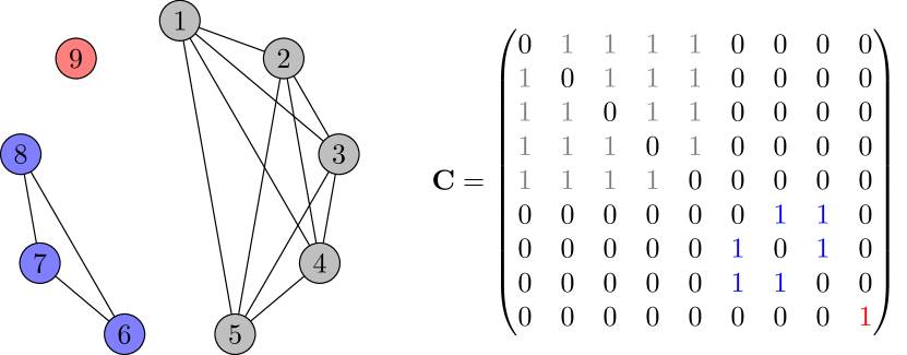
Figure 1: Chromosome expressed in a cluster graph representation. Here, 9 normal modes, corresponding to the graph vertexes, are grouped into three subspaces (gray, blue, and red), containing 5, 3, and 1 modes, respectively. Each subspace is a fully connected graph (a clique), and there is no interaction between any two subspaces. On the right, the corresponding adjacency matrix is colored accordingly.

All the information about the subspaces is codified in the adjacency matrix $\mathbf{C}$. It is defined by $C_{ij}=1$ only if modes $i$ and $j$ are in the same subspace, otherwise $C_{ij}=0$. $C_{ii}=1$ only if mode $i$ is in a one-dimensional subspace. In the end, we have increased the problem variables from the $F$-dimensional redundant representation (such as in the linear representation (1,2,3,4,5)(6,7,8)(9)=(2,4,1,5,3)(8,7,6)(9)=…) to the $F(F+1)/2$-dimensional non-redundant one. The $F$-dimensional representation is redundant because any mode permutation within a given subspace leaves the subspace unaffected. Our adjacency matrix representation is invariant to row and column permutation within the subspace block. Hence, every subspace configuration has a unique adjacency matrix representation. Furthermore, our adjacency matrix is symmetric, thus completely defined by its F(F+1)/2 lower (upper) triangular elements.

Secondly, we customize the crossover and mutation operators to mix the chromosomes with simple arithmetic rules and store the genetic information in a matrix of weights $\mathbf{\Phi}(\tau)$, which represents the probability distribution of the mixed chromosomes at the evolution epoch $\tau$. We define the crossover $\mathcal{X}$ of a couple of chromosomes $C$ and $C^{\prime}$ as a weighted average of their adjacency matrices

$$\mathcal{X}=\dfrac{1}{w_{C}+w_{C^{\prime}}}\left(w_{C}\mathbf{C}+w_{C^{\prime}}\mathbf{C}^{\prime})\right),$$ (12)

where $\mathbf{C}$ and $\mathbf{C}^{\prime}$ are adjacency matrices and the weights $w_{C}$ and $w_{C^{\prime}}$ depend on the chromosome fitnesses. The pure mutation $\mathcal{M}$ of a chromosome $C$ with probability $\mu$ is

$$\mathcal{M}=\dfrac{1}{1+F\mu}\left(\mathbf{1}\mu+\mathbf{C}\right),$$ (13)

where $\mathbf{1}$ is the square matrix of ones and $F$ is the number of genes. In our approach each vibrational normal mode corresponds to a gene, as illustrated in the previous example of Fig. 1. Both crossover and mutation have the basic property of scattering the gene probability. More specifically, the crossover distributes the probability among the genes expressed in $C$ and $C^{\prime}$, depending on their fitness, and the mutation distributes it among every possible outcome, independently of the fitness and the expression. The combination of the crossover and mutation processes is obtained by the subsequent application of the two operations: the mutation can be equivalently applied to the single chromosomes previous to undergoing crossover, or to the result of the crossover process. In addition, considering that we use $m$ chromosomes for the optimization, only an elite fraction $\eta<1$ of these are the fittest chromosomes that undergo the crossover and mutation processes. Eventually, the resulting probability distribution at epoch $\tau$, $\mathbf{\Phi}(\tau)$, is:

$$\mathbf{\Phi}(\tau)=\dfrac{1}{1+F\mu}\left[\mathbf{1\mu}+\dfrac{1}{\sum_{i}^{m\eta}w_{i}}\sum_{i=1}^{m\eta}w_{i}\mathbf{C}_{i}\right],$$ (14)

where $\text{C}_{i}$ is the $i$-th chromosome adjacency matrix and the new probability distribution is essentially generated by suitably mixing the adjacency matrices of the previous generation. This is the machine learning part, where the algorithm, epoch by epoch, learns the optimal probability distribution from an evolving population of chromosomes. For this work we use the simple weighting scheme $w_{i}=(m\eta-i)/m\eta$ with the resulting normalization constant $\sum_{i}^{m\eta}w_{i}=(m\eta-1)/2$, the elite fraction is $\text{$\eta$}=0.4$, while the mutation probability $\mu$ and the number of chromosomes will be specified below case by case. $\mathbf{\Phi}(\tau)$ is updated at every epoch and contains the average genetic material of the previous generation of chromosomes according to Eq. (14).

To sample new chromosomes from the probability distribution, $\mathbf{\Phi(\tau)}$ must be normalized. For the expression in Eq. (14), this means that $\mathbf{\Phi(\tau)}$ has to be symmetric and doubly stochastic, i.e. with rows and columns summing up to 1, so that we can consider $\mathbf{\Phi(\tau)}$ a weighted undirected graph to sample from. To enforce the doubly stochastic property and, at the same time, retain the symmetry, we rely on Sinkhorn’s theorem,Sinkhorn and Knopp (1967) which ensures that there exist two diagonal matrices $\mathbf{R}$ and $\mathbf{S}$ such that $\mathbf{R}\mathbf{\Phi}(\tau)\mathbf{S}$ is doubly stochastic. $R_{ii}$ and $S_{jj}$ are found by repeatedly and alternatively normalizing the rows and the columns of $\mathbf{\Phi}(\tau)$, according to the updates

$$\begin{split}R_{ii}&=\dfrac{1}{\sum_{j}\Phi_{ij}(\tau)S_{jj}}\quad\ \forall\ i\\ S_{jj}&=\dfrac{1}{\sum_{i}\Phi_{ij}(\tau)R_{ii}}\quad\ \forall\ j\ ,\end{split}$$ (15)

with $S_{jj}$ initialized to 1 for all $j$. $\mathbf{R}$ and $\mathbf{S}$ will converge, up to a small threshold $\varepsilon$, after an unspecified number of iterationsSinkhorn and Knopp (1967). In all the applications described below we use $\varepsilon=10^{-8}$ on each element of $\mathbf{R}$ as and $\mathbf{S}$, which is always satisfied in less than 100 iterations.

Third, we need to elaborate a procedure for obtaining the newborn chromosomes from the symmetric and doubly stochastic probability matrix $\mathbf{\Phi}(\tau)$. To sample representative cluster graphs from $\mathbf{\Phi}(\tau)$, we propose a sampling procedure to generate a population which reflects the original distribution:

1. generate the random numbers $r_{i},i=1,2,\dots F$ and sample independently the chances of each mode to be in a subspace alone. If $r_{i}<\Phi_{ii}(\tau)$ then the normal mode $i$ is in a subspace alone;

2. iterate on the leftover modes in a random order: if the $k$-th mode is already joined with another mode, then continue with the next one, otherwise sample the edge between modes $k$ and $j\neq k$ with a random number and join them with a probability given by the matrix element $\Phi_{jk}(\tau)$. If the $k$-th cannot be joined to any $j$ (for instance, because each of them is in a one-dimensional subspace) it stays in a subspace by itself;

3. identify the connected components of the sampled graph and complete them, obtaining the cluster graph for a newborn chromosome.

Note that before step 3, the procedure samples tree graphs, which means that there are no redundant sampling steps. Each chromosome sampled with this procedure may be weakly biased anyway and the random shuffle of the mode order in step 2 is required to make the sampled population representative and the overall sampling unbiased. To achieve step $3$ we look for a basis of the Laplacian matrix Kernel, with the Laplacian matrix defined as $L_{ij}=-C_{ij}+\delta_{ij}\sum_{j}C_{ij}$. Since $\sum_{j}L_{ij}=0$ by definition, the vector of ones always belongs to $Ker(\mathbf{L})$, i.e. to the collection of vectors x such that $\mathbf{Lx}=\bm{0}$. Furthermore, if the graph is disconnected, $\mathbf{L}$ can be rearranged to be block diagonal by swapping row and column indexes, with each block being the Laplacian of the corresponding connected subgraph. Hence each basis vector of $Ker(\mathbf{L})$ is 1 on the entries of the connected vertices and 0 elsewhere. The sum of all basis vectors is the vector of ones. To practically find a basis for $Ker(\mathbf{L})$ we solve the linear equation $\mathbf{Lx}=\bm{0}$ by applying Gaussian EliminationHigham (2011) to the augmented matrix $\mathbf{L}|\mathbf{I}$, with output $\mathbf{L_{rref}|B}$, where $\mathbf{L_{rref}}$ is the reduced row echelon form of $\mathbf{L}$. The rows $\mathbf{x}$ in $\mathbf{B}$ corresponding to the row indices where $\mathbf{L_{rref}}=\bm{0}$ do solve the linear equation and hence form a basis for the kernel.

To measure the likelihood of a subspace $s$ of size $D$ sampled from $\mathbf{\Phi}(\tau)$, we sum the edge products of all the possible trees that span the clique (subspace), as

$$p(s,\tau)=\frac{(D-1)^{D-1}}{D^{D-2}}\sum_{\mathbf{T}\in span(\tilde{\mathbf{\Phi}}_{s}(\tau))}\prod_{e=1}^{D}T_{e},$$ (16)

where $T_{e}$ is the edge of the tree graph $\mathbf{T}$, which spans the subspace probability distribution $\tilde{\mathbf{\Phi}}_{s}(\tau)$ (that is the probability distribution considering only the modes in $s$). The first factor is a normalization constant so that $p(s,\tau)$ does not depend on the subspace size and it is maximized to 1 when $\tilde{\mathbf{\Phi}}_{s}(\tau)$ is uniform. $D^{D-2}$ is the number of spanning trees for a clique according to Cayley’s formula.Cayley (1889) $p(s,\tau)$ measures the degree of convergence towards the chosen subspace $s$, such that, as $p(s,\tau)$ approaches unity, the population becomes more and more uniform and eventually the algorithm stops learning. The brute force application of Eq. (16) is out of reach for large subspaces ($D>\approx 10$), therefore, we use it only to check the algorithm progression towards an optimal solution of the small systems described below. Furthermore, GAs in general, and PG-EA in particular, do not require a full convergence of the population for the solution to be satisfactory. On the contrary, if the solution is unknown or hard to find, a homogeneous population is undesirable, as it kills diversity and damps the optimization.

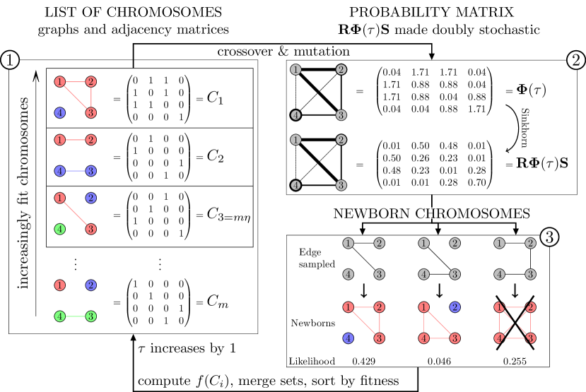
Figure 2: A numerical example of the PG-EA for a four dimensional system. The procedure is broken down into 3 steps. The inner rectangle in panel 1 includes the $m\eta$ elite chromosomes which will be employed for mutation and crossover in panel 2.

In Fig. (2) we report a four normal mode example to show how the PG-EA algorithm works in practice. First, as we do in all our simulations, the initial probability distribution is set as $\Phi_{ij}(0)=1/F\ \forall\ i,j$. Then, we generate the initial chromosome population according to the sampling procedure described at points 1-3 above. Each chromosome graph is reported together with the corresponding adjacency matrix in panel 1 in the left side of Fig. (2). The chromosomes $C_{j}$ are ordered by the fitness score, which is calculated using the function $f\left(C\right)$ (pay attention that according to our definition of the fitness function, Eq. 11, the preferred chromosomes are those with lower fitness score). The chromosome fraction $m\eta$ undergoes crossings and mutations. We reject (i.e. apply an infinite penalty) to any subspace which has a dimension larger than the largest subspace value $\bar{D}$ that one fixes a priori. Since assigning the fitness score is the most expensive step, it is advisable to build a score database, i.e. a list of already known chromosomes with their fitness value, so that, whenever a known chromosome is encountered its score does not have to be recomputed. After undertaking crossovers and mutations according to Eq. (14), a new (non-normalized) probability distribution is generated (panel 2 on the right side of Fig. 2). After transforming the new probability distribution into a symmetric and doubly stochastic distribution matrix using Sinkhorn’s algorithm, we generate the newborn chromosomes according to the sampling procedure of points 1-3 described above. A likelihood coefficient is calculated according to Eq. (16). In the lower right part of Fig. 2, the 4-dimensional solution is rejected because its dimensionality is greater than the largest subspace value $\bar{D}$, which in this numerical example has been fixed to be $\bar{D}=3$. Finally, a fitness coefficient is attributed to each chromosome and we are back to panel 1 for the next iteration. At each epoch, the fittest $i$-th chromosome, i.e. the one with the lowest $f\left(C_{i}\right)$ value, provides the graph with the so far optimal normal modes arrangement into subspaces.

II.3 2-mode interaction method

As an alternative, we propose an approximate and computationally cheaper method to deal with large molecules when the computational cost of PG-GA is prohibitive or in instances in which one can reasonably assume that for each normal mode the coupling is mainly due to the interaction with just a second mode.

In this alternative approach, we first compute a 2-mode coupling network, where each vertex $i,j$ is a normal mode and each edge is weighted by the two-mode Jacobian determinant $G_{ij}=\det(\tilde{\mathbf{J}}_{ij})$. $\tilde{\mathbf{J}}_{ij}$ is a $4\times 4$ matrix containing all the partial derivatives between the phase-space momenta and positions of modes $i$ and $j$ with respect to the initial conditions. For each full-dimensional Jacobian matrix $\mathbf{J}$ along the trajectory, we evaluate the determinant of every two-mode combination, $G_{ij}$. Then, we compute the distance matrix $\mathbf{E}=|\mathbf{G}-\mathbf{1}|$, which measures how large is the error done by assuming that the relevant interaction is only between the couple (i,j) of modes while other interactions are disregarded. Specifically, when $E_{ij}=0$, then modes $i$ and $j$ are fully correlated and uncoupled to any other mode. $\mathbf{E}$ is computed at every time step of the test trajectory and all $\mathbf{E}$ matrices are averaged into a single distance matrix representative of the whole trajectory.

Then, we employ an agglomerative hierarchical clustering technique called Weighted Pair Group Method with Arithmetic mean (WPGMA) Sokal (1958) to cluster the normal modes using the information encoded in $\mathbf{E}.$ The algorithm produces a dendrogram where each branching is an optimal subspace. Among the several hierarchical clustering techniques available in the literature, we choose WPGMA because it provides results which are the closest to the exact ones for the model systems considered below. WPGMA clustering is iterative and hierarchical. To start, each mode is in a subspace by itself. Then, at every iteration, the two ”closest” subspaces are merged into one and the dendrogram profile shows a link. The distance between the newly formed subspace $(j\cup k)$ and a given subspace $i$ is calculated as the arithmetic mean of the distances from the newly merged subspaces $j$ and $k$:

$$E^{\prime}_{i(j\cup k)}=\dfrac{E_{ij}+E_{ik}}{2}.$$ (17)

The procedure goes on until a maximum distance criterion has been met, i.e. until all modes fall into one large subspace.

The whole process is represented by a dendrogram, where each node corresponds to a subspace and each edge represents the link between two subspaces. At the root of the dendrogram there is the full-dimensional system, which contains all modes. The leaves are the subspaces containing one mode only. The distance $E_{ij}$ of every update is a measure of how close the linked subspaces are. Finally, this process generates a number of arrangements of normal modes at different level of the tree, and for every such arrangement we measure the fitness score, i.e. the full-dimensional Jacobian factorization error with Eq. (11), along with $E_{ij}$.

III Results

This section presents our results and it can be divided into three parts. In Sec. III.1, we show how PG-EA and the 2-mode interaction method are effective when applied to model systems like coupled Morse oscillators with non-trivial coupling topologies but obvious mode separations. In subsection III.2, we show that we can improve spectra accuracy with respect to previous calculations where the hierarchical subspace optimization originally proposed was adopted.Di Liberto, Conte, and Ceotto (2018a) Finally, in subsection III.3 we show that PG-EA allows us to apply the DC-SCIVR method and select the subspaces with the Jacobi criterion even for simulation of mid-large molecules such as the 12-atom trans-N-Methylacetamide. Remarkably, it would not have been possible to accomplish this task with a brute force combinatorial approach.

III.1 Model systems

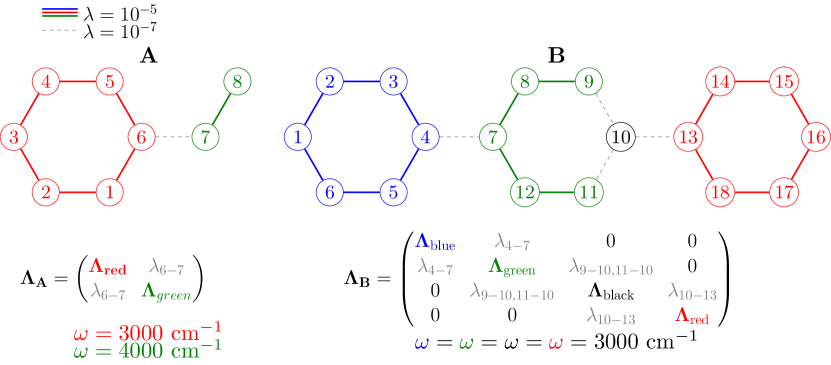
Figure 3: Toy model systems with different coupling topologies. The circled numbers represent Morse oscillators and the edges their couplings. When two oscillators are not connected by an edge, the relative coupling matrix element $\lambda_{ij}$ is zero. The oscillator frequencies $\omega$, reported below each coupling matrix, are 3000 $\leavevmode\nobreak\ \mathrm{cm}^{-1}$ except for modes 7 and 8 of topology A, for which $\omega=4000\leavevmode\nobreak\ \mathrm{cm}^{-1}$. Note that for topology A reported on the left, oscillators 1 and 5 are equivalent and they produce the same signal, as well as 2 and 4. Similar symmetry considerations can be applied to topology B.

To preliminarily test our algorithms, we consider the arrangements of $F$ coupled Morse oscillators A and B in figure 3. Each oscillator experiences the following Morse-type potential

$$V^{morse}= \sum_{i=1}^{F}D_{e}\left(1-e^{-\omega_{i}(2D_{e})^{-1/2}(q_{i}-q_{eq,i})}\right)^{2}+$$ (18)

$$\sum_{i=1}^{F-1}\sum_{j>i}^{F}\lambda_{ij}(q_{i}-q_{eq,i})(q_{j}-q_{eq,j}),$$

where the dissociation energy $D_{e}=38293\leavevmode\nobreak\ \mathrm{cm}^{-1}$ and the equilibrium position $q_{eq}=1.4\>\text{a.u.}$ are valid for all $F$ degrees of freedom. According to the coupling graphs and matrices $\mathbf{\Lambda}$ schematically represented in Figure 3, the oscillators might be uncoupled (no edge), weakly coupled ($\lambda=10^{-7}\>\text{a.u.}$, dashed edge) or strongly coupled ($\lambda=10^{-5}\>\text{a.u.}$, solid edge). We devise two topologies (A and B) to provide non-trivial examples. A has oscillator frequency $\omega=3000\>\text{cm}^{-1}$ for the oscillators 1 through 6 and $\omega=4000\>\text{cm}^{-1}$ for oscillators 7 and 8; B has all oscillators with the same frequency $\omega=3000\>\text{cm}^{-1}$. In both cases the correct separation into subspaces is unique.

Both PG-EA and the 2-mode interaction method separate system A correctly. In PG-EA we use $m=50$ chromosomes, mutation probability $\mu=0.001$, crossover fraction $\eta=0.4$ and 70 epochs, with the constraint that the maximum dimension is $\bar{D}=6$. The likelihood of the optimal subspaces calculated using Eq. (16) is plotted against the epochs in panel (a) at the top left of Fig. 4, showing that the population quickly converges to the unique global optimum represented by the continuous lines. The 2-mode interaction method provides three choices for the subspaces, the best of which is the global optimum (1,2,3,4,5,6)(7,8), reported in the first branching of the dendrogram in panel (b) at the top right of Fig. 4. This global optimum has a Jacobian factorization error of about $3.37\cdot 10^{-6}$. The example of topology B is much more challenging, as it is an 18-dimensional system divided in 4 loosely connected regions, one of which containing a single mode. As expected, it turns out that the best subspace division has oscillator 10 (black subspace in Fig. 3) joined together with five oscillators (7-12, green subspace), since there is one term less in the fitness function summation with respect to the case in which oscillator 10 is left isolated. In panel (c) at the bottom left of Fig. (4), PG-EA provides the optimal desired solution using $m=300$ chromosomes, $\mu=0.1$, $\eta=0.4$ and 1000 epochs, with the constraint that the largest subspace dimension is $\bar{D}=10$. In panel (d) at the bottom right of Fig. 4, the 2-mode interaction method also provides the optimal solution, as shown in the upper part of the dendrogram with the smallest Jacobian factorization error.

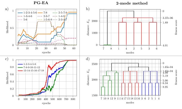
Figure 4: Vibrational modes subdivision optimizations of the model systems in Fig. (3) using PG-EA (left panels (a) and (c)) and the 2-modes interaction method (right panels (b) and (d)). In the top panels ((a) and (b)) the subspace optimizations of topology A is effectively achieved using both methods. The dendrogram (panel (b)) is colored to highlight the least error branching. In the bottom panels (panels (c) and (d)) the subspace optimization is effectively reached by both methods for topology B.

Now, one may wonder if these subdivisions are indeed the most suitable ones for DC-SCIVR spectroscopic calculations. In Figure 5 we show that DC SCIVR can account properly for most of the spectral features of these systems, if the subspaces are chosen accordingly to the algorithms described above. For example when choosing the subspace separation (1,3,5,8)(2,4,6,7), which is the least fit for case A i.e. it has the largest fitness score in case of requiring 2 subspaces only, the corresponding spectra are quite noisy as shown in Figure 5. Furthermore, phantom signals are observed, for example at $2686\>\text{cm}^{-1}$. Conversely, the spectra of the subspaces suggested by both our algorithms, which are reported with green and red lines, are without noise to the naked eye. However, we notice that the signal originated from a combination band of modes from different subspaces at $7006\>cm^{-1}$ is too weak in this scale to be observed. This is not a drawback of the algorithms proposed in this work, but a known feature of the DC-SCIVR method in predicting mixed overtones originated from modes belonging to different subspaces.

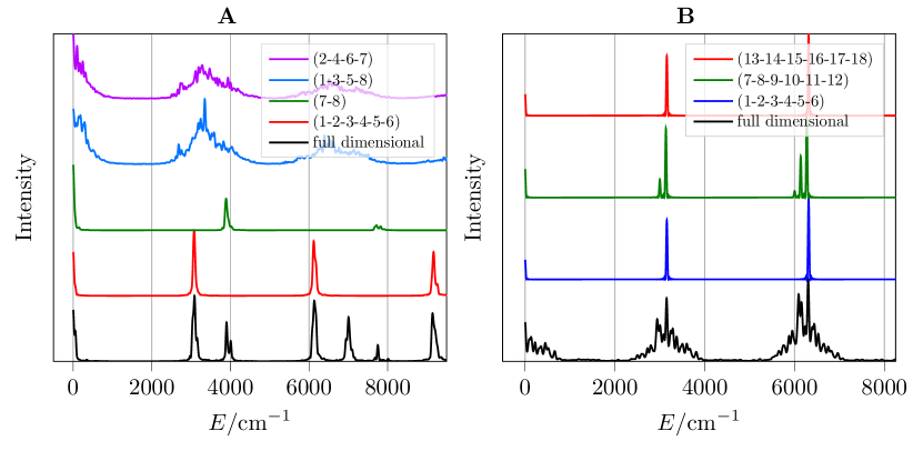
Figure 5: Spectra of the coupling topologies A and B of Morse oscillators with ZPE signals shifted to 0 $\mathrm{cm^{-1}}$. Left panel for system A: in black the full-dimensional spectrum; in red and green the best subspaces (ring and segment respectively with reference to figure 3), while the blue and purple are the two worst subspaces. Right panel for system B: in blue, dark green and red the best subspaces; in black the full-dimensional calculation.

On the right part of Fig. 5 we show the optimal subspace spectra for system B. In this case, the system is too large to have a well-converged semiclassical full-dimensional TA-SCIVR spectrum as shown by the black continuous line spectrumCeotto, Tantardini, and Aspuru-Guzik (2011). Instead, it is possible to recover the most significant spectroscopic features of the system with a DC-SCIVR calculation based on the optimal subspaces suggested by the algorithms.

III.2 The CH4 Molecule

This section further confirms the ability of the proposed algorithms to find optimal subspace separations for DC-SCIVR calculations when applied to real systems. We show that our techniques can reproduce and improve the DC-SCIVR spectra even for small molecules. We consider CH4 as the case system. Methane vibrational spectrum is a tough challenge for DC SCIVR because the molecule is characterized by highly chaotic dynamics and high symmetry which is difficult to recover if a proper subspace partition is not implemented. We simulate 180000 trajectories 30000 a.u. long and each trajectory is rejected if during the dynamics $||\det(\mathbf{J}^{T}\mathbf{J})|-1|>10^{-5}$. The initial trajectory conditions are sampled from the Husimi distribution centered in phase space at $(\sqrt{\bm{\omega}},\mathbf{q}_{eq})$, while gradients and Hessian matrices are computed by finite differences with infinitesimal displacements equal to $10^{-3}$ a.u. for all modes.

We use the Force-Field by Lee, Martin and Taylor Lee, Martin, and Taylor (1995) which takes into account the symmetry relations of cubic and quartic force constants. Gray and Robiette (1979); Raynes et al. (1987) The same PES and the hierarchical subspace optimization with the Jacobi method was employed in a previous work of the group.Ceotto, Di Liberto, and Conte (2017) For this system PG-EA successfully converges with the constraint $\bar{D}\leq 7$, which leads to the optimal couple of subspaces (2,5)(1,3,4,6,7,8,9), with a fitness score of about 0.71. The three subspaces (1)(2,3)(4,5,6,7,8,9) were selected in a previous work of the group Ceotto, Di Liberto, and Conte (2017) using the Jacobi criterion but looking for optimal subspaces with a brute force hierarchical approach and constraining the largest subspace to be six dimensional. These three subspaces have an associated fitness score of about 0.91. For methane PG-EA converges using $m=100$ chromosomes, $\eta=0.4$, $\mu=0.01$ and 50 epochs. The Likelihood plot is represented in panel (a) in the left part of figure 6.

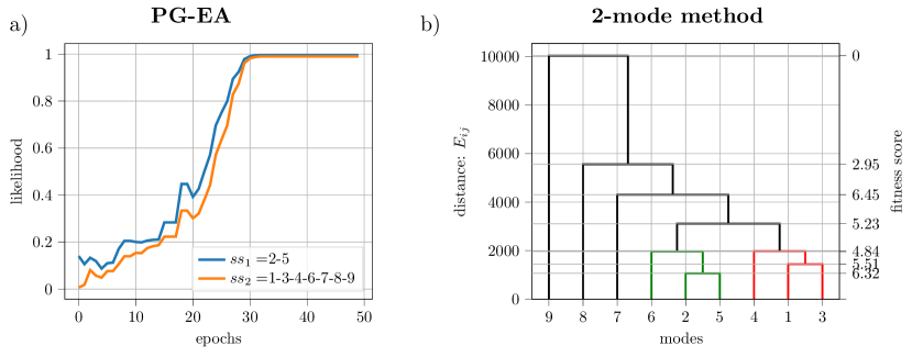
Figure 6: Likelihood of the optimal subspaces of methane during PG-EA optimization (panel (a)) and dendrogram for separation with 2-mode approximation method (panel (b)). Note that the 2-mode approximation leads to a very different result.

As shown in Fig. 6 (panel (b)), the 2-mode approximation leads, in this case, to a poor subspace separation: the best branch in the dendrogram is the colored (1,3,4)(2,5,6)(7)(8)(9) with a score of 4.84, leading to a bigger error than PG-EA for the Jacobian factorization.

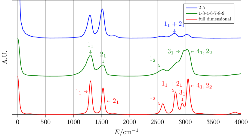
Figure 7: Spectrum of methane: the full-dimensional spectrum is in red; the reduced dimensionality spectra chosen according to PG-EA are in green and blue.

Methane, in absence of a preliminary adiabatic switching sampling,Conte et al. (2019) is known to be characterized by highly chaotic dynamics, Lee, Martin, and Taylor (1995) thus we employed 180000 trajectories to provide convergent results, with a rejection rate of about 90%, keeping nearly 2000 trajectories per degree of freedom. Fig. 7 reports both the full-dimensional spectrum (red continuous line) and the partial dimensional ones (green and blue), according to the PG-EA vibrational space sub-division found above. All spectroscopic features are properly reproduced. Note that degenerate modes belonging to different subspaces give rise to spectral lines at the same energy (see for instance $1_{1}$ and $2_{1}$ signals displayed in both subspace spectra in Fig. 7). In these cases, we consider more accurate the peaks appearing in the largest subspace, as more mode interactions are taken into account, even if frequencies of degenerate modes in different subspaces are very similar and cannot be distinguished by naked eye. In Fig. 7 we employ an incremental notation for the spectral features, so that degenerate signals are collected together under the same label. For a deeper insight, we report in Tab. 1 the value in wavenumbers of each spectral peak frequency.

Table 1: Quantum frequencies of vibration of the methane molecule in $\mathrm{cm}^{-1}$ calculated on the PES by Lee, Martin and Taylor Lee, Martin, and Taylor (1995) using full-dimensional TA SCIVR, DC-SCIVR based on PG-EA subspace partition, and discrete variable representation calculations (Exact). MAE stands for Mean Absolute Error, calculated using exact (MAE (Exact)) or full-dimensional semiclassical values (MAE (TA SCIVR)) as reference. In the fourth column, we report the DC-SCIVR frequencies obtained from the subdivision proposed in Ref.11 where a different approach for the Jacobi method was employed.

Incremental label	Modes (symmetry)	Exact Carter, Shnider, and Bowman (1999)	TA SCIVR	DC SCIVR (1)(2,3)(4-9)Di Liberto, Conte, and Ceotto (2018a)	DC SCIVR PG-EA (2,5)(1,3,4,5-9) [sub]a
$1_{1}$	1,2,3 $(F_{2})$	1313	1304	1287	1305 [G]
$2_{1}$	4,5 $(E)$	1535	1529	1534	1530 [G]
$1_{2}$	1,2,3	2624	2600	2562	2610 [G]
$1_{1}+2_{1}$	1,2,3,4,5	2836	2827		2807 [B]
$3_{1}$	6 $(A_{1})$	2949	2948	2960	2980 [G]
$4_{1}$	7,8,9 $(F_{2})$	3053	3051	3044	3036 [G]
$2_{2}$	4,5	3067	3051	3044	3036 [G]
MAE (Exact)			9.6	22.0	19.3
MAE (TA SCIVR)				14.3	13.4

^asubspace from which the wavenumber is taken: G for the 7-D green one and B for 2-D blue one with reference to Figure 7

In conclusion, PG-EA provides a subdivision of the vibrational space appropriate for DC-SCIVR spectroscopic calculations and we can move to apply it to larger systems where previous recipes for vibrational space subdivision are impracticle.

III.3 Trans-N-Methylacetamide

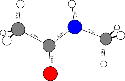
Figure 8: trans-N-Methylacetamide equilibrium geometry on the Potential Energy Surface by Nandi, Qu, and Bowman.Qu and Bowman (2019) Representative bond lengths of the equilibrium geometry are shown in Ångström. The HNCO peptide bond is of fundamental importance for the dynamics of peptides.

Here we present the subspace optimization and the associated DC-SCIVR spectroscopic calculations for the 30-mode trans-N-Methylacetamide (NMA) molecule represented in Fig. 8. NMA has been studied thoroughly both computationally Chen et al. (1995); Kubelka and Keiderling (2001); Torii et al. (1998) and experimentally Ataka, Takeuchi, and Tasumi (1984); Mayne and Hudson (1991); Chen et al. (1995); Torii et al. (1998); Triggs and Valentini (1992), as it is one of the simplest examples of a molecule featuring the HNCO peptide bond. We use the full-PES by Nandi, Qu and BowmanQu and Bowman (2019), which has been designed both for cis- and trans- NMA and that accounts for the three-fold symmetry of the methyl rotors. The PES is permutationally invariant and was fitted to thousands of ab initio calculated energies and gradients at B3LYP/cc-pVDZ level of theory.Qu and Bowman (2019) In this case we can compare our DC-SCIVR spectroscopic results with harmonic frequencies and gas phase IR and Raman experimental values.Ataka, Takeuchi, and Tasumi (1984)

The two methyl rotational frequencies, i.e. the two lowest-frequency normal mode values, are not considered to be part of the vibrational space. Thus, the dimensionality of the vibrational space we consider is 28. We use a simulation time step of 5 a.u. The finite difference displacement of the $i$-th normal mode for Hessian and gradients is rescaled by $10^{-3}\sqrt{\max(\bm{\omega})/\mathbf{\omega}_{i}}$,Cazzaniga et al. (2020) to account for different PES curvatures along each one of the normal mode coordinates. We use the signal obtained from a single 30000 a.u. long trajectory with initial conditions $(\sqrt{\bm{\omega}},\mathbf{q}_{eq})$. We do not observe any conformational change from the trans to the cis potential energy basin during our simulations.

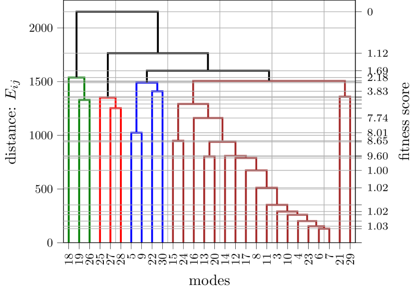
Figure 9: 2-mode interaction dendrogram of trans-NMA. Four subspaces are generated with a Jacobian factorization score equal to 2.18. As an alternative, one might prefer the five-subspace option with an error of 3.83. We do not show the likelihood vs epochs plot, since the convergence of the whole population is not achieved nor desired. Furthermore computing the likelihood in Eq. 16 for a 12 dimensional subspaces is not feasible as it requires the computation of $12^{10}$ products.

We apply PG-EA, the 2-mode interaction method, and the Hessian methodDi Liberto, Conte, and Ceotto (2018a) to divide the vibrational space into subspaces. The results are quite different. For PG-EA, we run a thorough optimization using 10000 epochs, $m=300$ chromosomes, $\mu=0.01$ and $\eta=0.4$, with the largest subspace constraint set to $\bar{D}=15$ and we obtain the following three subspaces: A = (3,5,7,10,11,12,15,21,23,26,28,30), B = (4,9,14,16,17,18,19,22,24,25,27,29) and C = (6,8,13,20). The fitness score of the chromosome, i.e. the score of the Jacobian factorization, is 1.96. When applying the basic average Hessian criterionDi Liberto, Conte, and Ceotto (2018a) with a corse-graining parameter equal to $8\cdot 10^{-6}$, we obtain the following subspaces: $a=$(3,5,7,22), $b=$(10,11,13,16,17,18,20,24,25,26,27,28,29), $c=$(4), $d=$(6), $e=$(8), $f=$(9), $g=$(12), $h=$(14), $i=$(15), $j=$(19), $k=$(21), $l=$(23), $m=$(30), which can be associated to a fitness score equal to 4.49. Finally, we apply the 2-mode dendogram approach and obtain the following subspaces: $\alpha=$(3,4,6,7,8,10,11,12,13,14,15,16,17,20,21,23,24,29), $\beta=$(5,9,22,30), $\gamma=$(18,19,26), $\delta=$(25,27,28) with a fitness score of 2.18. The 2-mode interaction method produced the dendrogram reported in Figure 9, which has a slightly worse score than the PG-EA result. However, the presence of an 18-dimensional subspace makes this subdivision not convenient for Monte Carlo phase-space integration convergence. The Hessian method is instead clearly penalized by the many 1-D subspaces found. These considerations suggest that the PG-EA subdivision into three subspaces is indeed the best choice.

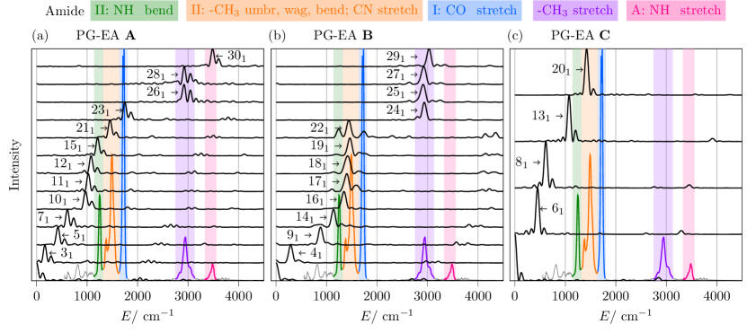
Figure 10: Panels (a), (b), and (c) are the three partial spectra for the three A, B, and C PG-EA subspaces. The colored spectrum is the experimental IR spectrum. Wallace (2020) The black continuous spectra are DC-SCIVR spectra calculated using different $\epsilon_{j}$ value (see Eq.(8)) for each normal mode of the subspace. Colored windows are for the different spectroscopic regions as denominated by experimentalists. These windows are commonly labeled Amide II (green and orange), Amide I (blue) and Amide A (pink). The purple window corresponds to CH3 stretching. Amide III, IV, and V bands are located below $\sim 1200\>\mathrm{cm}^{-1}$ and are very dependent on the side chains.

Based on PG-EA, we calculate the spectra reported in Fig. 10, where the different spectral regions are highlighted by different colors according to the experimentalists’ denomination. Overall, the DC-SCIVR spectra are reproducing well all the spectroscopic features of this molecule. Actually there are more spectral features in the DC-SCIVR simulation than there are in the experiment because DC SCIVR calculates the power spectrum, which is made of all vibrational levels (that we scale with respect to the zero-point energy), even those associated to transitions which are not IR active. An IR spectrum simulation with related intensities would require calculation of the vibrational eigenfunctions. This feature is not implemented yet in our divide-and-conquer approach, but we are planning to do it soon. In addition, according to our simulations and referring to the experimentalists’ denomination, mode 23 is the only one responsible for the Amide I band, subspace A contributes the most to amide III and A bands, while amide II is mostly localized in subspace B.

Table 2: Vibrational fundamental frequencies for trans-N-Methylacetamide (NMA). The first column denominates the vibrational modes. In the second column the fundamental frequencies in harmonic approximation (HO) are reported. DC SCIVR fundamental frequency of vibrations are obtained on the basis of subspace partition by means of PG-EA (third column), Hessian method (Hess, fourth column), and 2-mode interaction method (2-mode, fifth column). The results are sorted by increasing value of the harmonic frequencies and assigned by comparing the associated vibrational motion to the corresponding experimental description. Superscripts refer to the subspace each mode belongs to. The sixth column reports the ab-initio harmonic frequencies at the MP2/aug-cc-pVTZ level of theory (HO/MP2) .Kaledin and Bowman (2007) All data are compared by calculating the Mean Absolute Error (MAE) with respect to the experimental values (last column, Exp) by Ataka, Takeuchi and Tasumi.Ataka, Takeuchi, and Tasumi (1984)

	Frequency subID / $\mathrm{cm^{-1}}$
modes #	HO	DC SCIVR PG-EA (3 subs)	DC SCIVR Hess (12 subs)	DC SCIVR 2-mode (4 subs)	HO/MP2Kaledin and Bowman (2007)	Exp Ataka, Takeuchi, and Tasumi (1984)
3	150	163 A	159 a	156 α	151
4	290	289 B	285 c	283 α	259	279
5	393	421 A	417 a	416 β	347	429
6	433	451 C	451 d	448 α	423	439
7	621	609 A	608 a	606 α	630	619
8	629	613 C	611 e	612 α	633	658
9	866	881 B	875 f	871 β	883	857
10	995	967 A	970 b	972 α	1003	980
11	1038	1024 A	1028 b	1025 α	1058	1037
12	1112	1078 A	1080 g	1080 α	1119	1089
13	1132	1075 C	1069 b	1072 α	1169
14	1166	1137 B	1138 h	1134 α	1195	1168
15	1260	1208 A	1210 i	1205 α	1290	1266
16	1391	1345 B	1344 b	1347 α	1402	1370
17	1415	1401 B	1388 b	1388 α	1460	1419
18	1434	1418 B	1409 b	1415 γ	1487	1432
19	1474	1462 B	1463 j	1461 γ	1494	1446
20	1485	1422 C	1426 b	1430 α	1499	1432
21	1491	1453 A	1453 k	1453 α	1529	1472
22	1550	1441 B	1444 a	1472 β	1561	1511
23	1772	1774 A	1747 l	1745 α	1749	1707
24	3019	2936 B	2934 b	2920 α	3088	2915
25	3040	2914 B	2923 b	2919 δ	3091	2958
26	3072	2920 A	2903 b	2908 γ	3165	2916
27	3125	2926 B	2933 b	2924 δ	3188	3008
28	3126	2924 A	2912 b	2912 δ	3188	3008
29	3137	3030 B	3044 b	3037 α	3197	2973
30	3630	3485 A	3484 m	3485 β	3703	3498
MAE Exp	47.9	30.0	29.7	27.5	78.5

All these subspace choices produce spectra with almost the same MAEs, as reported in Tab. 2. This suggests that the subspace choice is flexible, as well as the choice of the subdivision criterion. However, PG-EA is the method that minimizes the number of subspaces and prevents from having many 1-D subspaces, which could result into a very noisy and not resolved spectrum.Cazzaniga et al. (2020)

A closer inspection of the vibrational frequency values in Tab 2 allows us to better understand the physical meaning of the MAE of the different methods, in particular of the Harmonic versus the DC-SCIVR one. In the case of the harmonic frequencies reported in the second column of Tab. (2), 22 out of 26 vibrational frequencies are higher than the experimental values. Thus, the MAE value of $48\>\text{cm}^{-1}$ is because of estimates by excess. In the case of the DC-SCIVR calculations it is the other way around. For example, 20 PG-EA values are underestimating the experimental frequencies and the MAE value of $\text{30\>cm}^{-1}$ is given by estimates by defect. Thus, the amount of anharmonic contribution introduced by the DC-SCIVR calculations is on average per mode $\sim 78\>\text{cm}^{-1}.$ This amount is comparable with the MAE under the column HO/MP2, where harmonic frequencies are calculated at a higher level of ab initio theory than the DFT-B3LYP/cc-pVDZ one. These considerations are suggesting that most probably, for this molecule, the discrepancies with respect to the experimental values are mainly due to the DFT level of ab initio theory. Conversely, only at a lower degree the inaccuracy can be related to the semiclassical approximation or the quality of the potential energy surface fitting, as previously shown on other systems.Conte, Botti, and Ceotto (2020) Unfortunately, a DC-SCIVR simulation at MP2/aug-cc-pVTZ level of ab initio theory is out of reach at time of writing due to its computational burden.

IV Summary and Conclusions

We have presented a machine learning algorithm based on a Probability Graph representation and an Evolutionary Algorithm procedure. The algorithm is able to find the best subdivision of the full-dimensional vibrational space into subspaces for model systems in which the best subspace division is known. Our approach is able to preserve Liouville’s theorem for each subspace as much as possible and for a given maximum dimensionality of the subspaces. We proved that the clustering provided by PE-GA is indeed one of the possible solutions that minimize the energy exchange between subspaces during the vibrational dynamics, and thus the most convenient for DC-SCIVR and spectroscopic calculations in general. As an alternative, we have proposed a 2-mode coupling scheme which is less computational intense but also less accurate. Application to the DC-SCIVR power spectrum calculation of trans N-Methylacetamide is made manageable under Liouville’s criterion restrictions only by means of these algorithms. The calculation of the DC-SCIVR power spectrum of trans-NMA with subspace division selected with Liouville’s criterion is manageable only employing these two algorithms.

The choice of the PG-EA parameters is arbitrary to some extent. As a matter of fact, the method is bound to look for new solutions at every epoch and hence it will get the global optimum, eventually. However, a sensible choice of the number of chromosomes and the mutation probability may significantly enhance the optimization. Assuming that the number of epochs is fixed, increasing the number of (elite) chromosomes means that the population evolves more slowly, enhancing the chances of eventually hitting the global optimum. However, as the evaluation of the fitness function is the most expensive step, a large population requires significantly more computational time. Conversely, using a small population means a fast evolution and therefore it is likely to obtain a fast local minimum. We suggest that a sensible choice of the mutation probability is in the interval [0.001, 0.2]. This parameter makes sure that the algorithm does not get stuck in a local minimum, even if the whole population is homogeneous. It becomes less and less important as the pool of possible solutions and the number of elite chromosomes increase.

There are several quantum methods that can take advantage from partitioning the nuclear vibrational degrees of freedom. Clearly, dividing the vibrational space into putative independent subspaces is an approximation. However, if this subdivision is performed according to Jacobi’s criterion, it may turn out not to be a rough approximation, especially for high dimensional and loosely connected systems. We believe that, at the affordable cost of a single adiabatic classical trajectory with Hessian calculation, the PG-EA algorithm can be useful to assist any method that has to deal with increasing computational costs with system dimensionality but that is able to perform accurate spectroscopic calculations for each subspace independently. This may be the case, for example, of the Local Mode variant of MultimodeWang and Bowman (2012); Liu, Wang, and Bowman (2012); Wang and Bowman (2013) or other semiclassical wavepacket propagation methods developed by other groups.Begusic, Roulet, and Vanicek (2018); Patoz, Begusic, and Vanicek (2018); Wehrle, Oberli, and Vaníček (2015)

The work we have presented provides a rigorous rationalization of the simplification of a larger dimensional problem into a set of lower dimensional ones. The examples illustrated in the paper demonstrate that reliable spectroscopic results are obtained if a rigorous strategy is employed to get to a reasonable subspace partition while a non-educated, unwise choice of subspaces may lead to inaccurate or unreliable results. Our algorithms might serve as a powerful tool for advancing the computational spectroscopy of large molecules.

AIP PUBLISHING DATA SHARING POLICY

The data that support the findings of this study are available from the corresponding author upon reasonable request.

References

- Holland (1962) J. H. Holland, “Outline for a logical theory of adaptive systems,” Journal of the ACM (JACM) 9, 297–314 (1962).
- Goldberg and Holland (1988) D. E. Goldberg and J. H. Holland, “Genetic algorithms and machine learning,” (1988).
- Holland et al. (1992) J. H. Holland et al., Adaptation in natural and artificial systems: an introductory analysis with applications to biology, control, and artificial intelligence (MIT press, 1992).
- Freeman and Xili (1987) R. Freeman and W. Xili, “Design of magnetic resonance experiments by genetic evolution,” Journal of Magnetic Resonance 75, 184–189 (1987).
- Hibbert (1993) D. B. Hibbert, “Genetic algorithms in chemistry,” Chemometrics and Intelligent Laboratory Systems 19, 277–293 (1993).
- Leardi (2001) R. Leardi, “Genetic algorithms in chemometrics and chemistry: a review,” Journal of Chemometrics: A Journal of the Chemometrics Society 15, 559–569 (2001).
- Niazi and Leardi (2012) A. Niazi and R. Leardi, “Genetic algorithms in chemometrics,” Journal of Chemometrics 26, 345–351 (2012).
- Beheshti et al. (2016) A. Beheshti, E. Pourbasheer, M. Nekoei, and S. Vahdani, “Qsar modeling of antimalarial activity of urea derivatives using genetic algorithm–multiple linear regressions,” Journal of Saudi Chemical Society 20, 282–290 (2016).
- Bhattacharya et al. (2009) B. Bhattacharya, G. D. Kumar, A. Agarwal, Ş. Erkoç, A. Singh, and N. Chakraborti, “Analyzing fe–zn system using molecular dynamics, evolutionary neural nets and multi-objective genetic algorithms,” Computational Materials Science 46, 821–827 (2009).
- Ceotto, Di Liberto, and Conte (2017) M. Ceotto, G. Di Liberto, and R. Conte, “Semiclassical "Divide-and-Conquer" Method for Spectroscopic Calculations of High Dimensional Molecular Systems,” Phys. Rev. Lett. 119, 010401 (2017).
- Di Liberto, Conte, and Ceotto (2018a) G. Di Liberto, R. Conte, and M. Ceotto, “"divide and conquer" semiclassical molecular dynamics: A practical method for spectroscopic calculations of high dimensional molecular systems,” J. Chem. Phys. 148, 014307 (2018a).
- Wehrle, Sulc, and Vanicek (2014) M. Wehrle, M. Sulc, and J. Vanicek, “On-the-fly ab initio semiclassical dynamics: Identifying degrees of freedom essential for emission spectra of oligothiophenes,” J. Chem. Phys. 140, 244114 (2014).
- Heller (1981a) E. J. Heller, “The semiclassical way to molecular spectroscopy,” Acc. Chem. Res. 14, 368–375 (1981a).
- Kaledin and Miller (2003a) A. L. Kaledin and W. H. Miller, “Time averaging the semiclassical initial value representation for the calculation of vibrational energy levels,” J. Chem. Phys. 118, 7174–7182 (2003a).
- Kaledin and Miller (2003b) A. L. Kaledin and W. H. Miller, “Time averaging the semiclassical initial value representation for the calculation of vibrational energy levels. ii. application to h2co, nh3, ch4, ch2d2,” J. Chem. Phys. 119, 3078–3084 (2003b).
- Miller (1968) W. H. Miller, “Uniform semiclassical approximations for elastic scattering and eigenvalue problems,” J. Chem. Phys. 48, 464–467 (1968).
- Miller (1971) W. H. Miller, “Semiclassical nature of atomic and molecular collisions,” Accounts of Chemical Research 4, 161–167 (1971).
- Miller (1998) W. H. Miller, “Spiers memorial lecture quantum and semiclassical theory of chemical reaction rates,” Faraday Discussions 110, 1–21 (1998).
- Miller (2001) W. H. Miller, “The semiclassical initial value representation: A potentially practical way for adding quantum effects to classical molecular dynamics simulations,” J. Phys. Chem. A 105, 2942–2955 (2001).
- Miller (2005) W. H. Miller, “Quantum dynamics of complex molecular systems,” Proc. Natl. Acad. Sci. USA 102, 6660–6664 (2005).
- Sun, Wang, and Miller (1998) X. Sun, H. Wang, and W. H. Miller, “On the semiclassical description of quantum coherence in thermal rate constants,” J. Chem. Phys. 109, 4190–4200 (1998).
- Thoss, Wang, and Miller (2001) M. Thoss, H. Wang, and W. H. Miller, “Generalized forward–backward initial value representation for the calculation of correlation functions in complex systems,” J. Chem. Phys. 114, 9220–9235 (2001).
- Yamamoto and Miller (2003) T. Yamamoto and W. H. Miller, “Semiclassical calculation of thermal rate constants in full Cartesian space: The benchmark reaction D+ H2 -> DH+ H,” J. Chem. Phys. 118, 2135–2152 (2003).
- Heller (1981b) E. J. Heller, “Frozen Gaussians: A very simple semiclassical approximation,” J. Chem. Phys. 75, 2923–2931 (1981b).
- Herman and Kluk (1984) M. F. Herman and E. Kluk, “A semiclassical justification for the use of non-spreading wavepackets in dynamics calculations,” Chem. Phys. 91, 27–34 (1984).
- Miller (2002) W. H. Miller, “An alternate derivation of the herman kluk (coherent state) semiclassical initial value representation of the time evolution operator,” Mol. Phys. 100, 397–400 (2002).
- Kluk, Herman, and Davis (1986) E. Kluk, M. F. Herman, and H. L. Davis, “Comparison of the propagation of semiclassical frozen Gaussian wave functions with quantum propagation for a highly excited anharmonic oscillator,” J. Chem. Phys. 84, 326–334 (1986).
- Kay (1994a) K. G. Kay, “Semiclassical propagation for multidimensional systems by an initial value method,” J. Chem. Phys. 101, 2250–2260 (1994a).
- Kay (1994b) K. G. Kay, “Integral expressions for the semiclassical time-dependent propagator,” J. Chem. Phys. 100, 4377–4392 (1994b).
- Kay (1994c) K. G. Kay, “Numerical study of semiclassical initial value methods for dynamics,” J. Chem. Phys. 100, 4432–4445 (1994c).
- Kay (2006) K. G. Kay, “The Herman–Kluk approximation: Derivation and semiclassical corrections,” Chem. Phys. 322, 3–12 (2006).
- Grossmann and Xavier (1998) F. Grossmann and A. L. Xavier, “From the coherent state path integral to a semiclassical initial value representation of the quantum mechanical propagator,” Phys. Lett. A 243, 243–248 (1998).
- Antipov, Ye, and Ananth (2015) S. V. Antipov, Z. Ye, and N. Ananth, J. Chem. Phys. 142, 184102 (2015).
- Church, Antipov, and Ananth (2017) M. S. Church, S. V. Antipov, and N. Ananth, “Validating and implementing modified filinov phase filtration in semiclassical dynamics,” J. Chem. Phys. 146, 234104 (2017).
- Church and Ananth (2019) M. S. Church and N. Ananth, “Semiclassical dynamics in the mixed quantum-classical limit,” J. Chem. Phys. 151, 134109 (2019).
- Buchholz et al. (2018) M. Buchholz, E. Fallacara, F. Gottwald, M. Ceotto, F. Grossmann, and S. D. Ivanov, “Herman-kluk propagator is free from zero-point energy leakage,” Chem. Phys. 515, 231–235 (2018).
- Heller (1991) E. J. Heller, J. Chem. Phys. 94, 2723–2729 (1991).
- Di Liberto and Ceotto (2016) G. Di Liberto and M. Ceotto, “The Importance of the Pre-exponential Factor in Semiclassical Molecular Dynamics,” J. Chem. Phys. 145, 144107 (2016).
- Ma et al. (2018) X. Ma, G. Di Liberto, R. Conte, W. L. Hase, and M. Ceotto, “A quantum mechanical insight into sn2 reactions: Semiclassical initial value representation calculations of vibrational features of the \ceCl-CH3Cl pre-reaction complex with the venus suite of codes,” J. Chem. Phys. 149, 164113 (2018).
- De Leon and Heller (1983) N. De Leon and E. J. Heller, “Semiclassical quantization and extraction of eigenfunctions using arbitrary trajectories,” J. Chem. Phys. 78, 4005–4017 (1983).
- Ceotto et al. (2009a) M. Ceotto, S. Atahan, G. F. Tantardini, and A. Aspuru-Guzik, “Multiple coherent states for first-principles semiclassical initial value representation molecular dynamics,” J. Chem. Phys. 130, 234113 (2009a).
- Ceotto et al. (2009b) M. Ceotto, S. Atahan, S. Shim, G. F. Tantardini, and A. Aspuru-Guzik, “First-principles semiclassical initial value representation molecular dynamics,” Phys. Chem. Chem. Phys. 11, 3861–3867 (2009b).
- Ceotto, Tantardini, and Aspuru-Guzik (2011) M. Ceotto, G. F. Tantardini, and A. Aspuru-Guzik, “Fighting the curse of dimensionality in first-principles semiclassical calculations: Non-local reference states for large number of dimensions,” J. Chem. Phys. 135, 214108 (2011).
- Gabas, Conte, and Ceotto (2017) F. Gabas, R. Conte, and M. Ceotto, “On-the-fly ab initio Semiclassical Calculation of Glycine Vibrational Spectrum,” J. Chem. Theory Comput. 13, 2378 (2017).
- Ceotto, Dell‘ Angelo, and Tantardini (2010) M. Ceotto, D. Dell‘ Angelo, and G. F. Tantardini, “Multiple coherent states semiclassical initial value representation spectra calculations of lateral interactions for CO on Cu (100),” J. Chem. Phys. 133, 054701 (2010).
- Conte, Aspuru-Guzik, and Ceotto (2013) R. Conte, A. Aspuru-Guzik, and M. Ceotto, “Reproducing Deep Tunneling Splittings, Resonances, and Quantum Frequencies in Vibrational Spectra From a Handful of Direct Ab Initio Semiclassical Trajectories,” J. Phys. Chem. Lett. 4, 3407–3412 (2013).
- Micciarelli et al. (2019) M. Micciarelli, F. Gabas, R. Conte, and M. Ceotto, “An effective semiclassical approach to ir spectroscopy,” J. Chem. Phys. 150, 184113 (2019).
- Micciarelli et al. (2018) M. Micciarelli, R. Conte, J. Suarez, and M. Ceotto, “Anharmonic vibrational eigenfunctions and infrared spectra from semiclassical molecular dynamics,” J. Chem. Phys. 149, 064115 (2018).
- Tamascelli et al. (2014) D. Tamascelli, F. S. Dambrosio, R. Conte, and M. Ceotto, “Graphics processing units accelerated semiclassical initial value representation molecular dynamics,” J. Chem. Phys. 140, 174109 (2014).
- Buchholz, Grossmann, and Ceotto (2016) M. Buchholz, F. Grossmann, and M. Ceotto, “Mixed semiclassical initial value representation time-averaging propagator for spectroscopic calculations,” J. Chem. Phys. 144, 094102 (2016).
- Buchholz, Grossmann, and Ceotto (2017) M. Buchholz, F. Grossmann, and M. Ceotto, “Application of the mixed time-averaging semiclassical initial value representation method to complex molecular spectra,” J. Chem. Phys. 147, 164110 (2017).
- Buchholz, Grossmann, and Ceotto (2018) M. Buchholz, F. Grossmann, and M. Ceotto, “Simplified approach to the mixed time-averaging semiclassical initial value representation for the calculation of dense vibrational spectra,” J. Chem. Phys. 148, 114107 (2018).
- Zhuang et al. (2012) Y. Zhuang, M. R. Siebert, W. L. Hase, K. G. Kay, and M. Ceotto, “Evaluating the Accuracy of Hessian Approximations for Direct Dynamics Simulations,” J. Chem. Theory Comput. 9, 54–64 (2012).
- Ceotto, Zhuang, and Hase (2013) M. Ceotto, Y. Zhuang, and W. L. Hase, “Accelerated direct semiclassical molecular dynamics using a compact finite difference Hessian scheme,” J. Chem. Phys. 138, 054116 (2013).
- Aieta et al. (2020) C. Aieta, M. Micciarelli, G. Bertaina, and M. Ceotto, “Anharmonic quantum nuclear densities from full dimensional vibrational eigenfunctions with application to protonated glycine,” Nature Communications 11, 1–9 (2020).
- Conte et al. (2019) R. Conte, L. Parma, C. Aieta, A. Rognoni, and M. Ceotto, “Improved semiclassical dynamics through adiabatic switching trajectory sampling,” J. Chem. Phys. 151, 214107 (2019).
- Di Liberto, Conte, and Ceotto (2018b) G. Di Liberto, R. Conte, and M. Ceotto, “"divide-and-conquer" semiclassical molecular dynamics: An application to water clusters,” J. Chem. Phys. 148, 104302 (2018b).
- Bertaina, Di Liberto, and Ceotto (2019) G. Bertaina, G. Di Liberto, and M. Ceotto, “Reduced rovibrational coupling cartesian dynamics for semiclassical calculations: Application to the spectrum of the zundel cation,” J. Chem. Phys. 151, 114307 (2019).
- Gabas et al. (2018) F. Gabas, G. Di Liberto, R. Conte, and M. Ceotto, “Protonated glycine supramolecular systems: the need for quantum dynamics,” Chem. Sci. 9, 7894–7901 (2018).
- Gabas, Di Liberto, and Ceotto (2019) F. Gabas, G. Di Liberto, and M. Ceotto, “Vibrational investigation of nucleobases by means of divide and conquer semiclassical dynamics,” J. Chem. Phys. 150, 224107 (2019).
- Gabas, Conte, and Ceotto (2020) F. Gabas, R. Conte, and M. Ceotto, “Semiclassical vibrational spectroscopy of biological molecules using force fields,” Journal of Chemical Theory and Computation (2020).
- Cazzaniga et al. (2020) M. Cazzaniga, M. Micciarelli, F. Moriggi, A. Mahmoud, F. Gabas, and M. Ceotto, “Anharmonic calculations of vibrational spectra for molecular adsorbates: A divide-and-conquer semiclassical molecular dynamics approach,” J. Chem. Phys. 152, 104104 (2020).
- Brewer, Hulme, and Manolopoulos (1997) M. L. Brewer, J. S. Hulme, and D. E. Manolopoulos, “Semiclassical dynamics in up to 15 coupled vibrational degrees of freedom,” J. Chem. Phys. 106, 4832–4839 (1997).
- Sinkhorn and Knopp (1967) R. Sinkhorn and P. Knopp, “Concerning nonnegative matrices and doubly stochastic matrices,” Pacific Journal of Mathematics 21, 343–348 (1967).
- Higham (2011) N. J. Higham, “Gaussian elimination,” Wiley Interdisciplinary Reviews: Computational Statistics 3, 230–238 (2011).
- Cayley (1889) A. Cayley, “A theorem on trees,” Quart. J. Math. 23, 376–378 (1889).
- Sokal (1958) R. R. Sokal, “A statistical method for evaluating systematic relationships.” Univ. Kansas, Sci. Bull. 38, 1409–1438 (1958).
- Lee, Martin, and Taylor (1995) T. J. Lee, J. M. Martin, and P. R. Taylor, “An accurate ab initio quartic force field and vibrational frequencies for CH4 and isotopomers,” J. Chem. Phys. 102, 254–261 (1995).
- Gray and Robiette (1979) D. Gray and A. Robiette, “The anharmonic force field and equilibrium structure of methane,” Molecular Physics 37, 1901–1920 (1979).
- Raynes et al. (1987) W. Raynes, P. Lazzeretti, R. Zanasi, A. Sadlej, and P. Fowler, “Calculations of the force field of the methane molecule,” Molecular Physics 60, 509–525 (1987).
- Carter, Shnider, and Bowman (1999) S. Carter, H. M. Shnider, and J. M. Bowman, “Variational calculations of rovibrational energies of CH4 and isotopomers in full dimensionality using an ab initio potential,” J. Chem. Phys. 110, 8417–8423 (1999).
- Qu and Bowman (2019) C. Qu and J. M. Bowman, “A fragmented, permutationally invariant polynomial approach for potential energy surfaces of large molecules: Application to n-methyl acetamide,” J. Chem. Phys. 150, 141101 (2019).
- Chen et al. (1995) X. Chen, R. Schweitzer-Stenner, S. A. Asher, N. G. Mirkin, and S. Krimm, “Vibrational assignments of trans-n-methylacetamide and some of its deuterated isotopomers from band decomposition of ir, visible, and resonance raman spectra,” The Journal of Physical Chemistry 99, 3074–3083 (1995).
- Kubelka and Keiderling (2001) J. Kubelka and T. A. Keiderling, “Ab initio calculation of amide carbonyl stretch vibrational frequencies in solution with modified basis sets. 1. n-methyl acetamide,” The Journal of Physical Chemistry A 105, 10922–10928 (2001).
- Torii et al. (1998) H. Torii, T. Tatsumi, T. Kanazawa, and M. Tasumi, “Effects of intermolecular hydrogen-bonding interactions on the amide i mode of n-methylacetamide: matrix-isolation infrared studies and ab initio molecular orbital calculations,” The Journal of Physical Chemistry B 102, 309–314 (1998).
- Ataka, Takeuchi, and Tasumi (1984) S. Ataka, H. Takeuchi, and M. Tasumi, “Infrared studies of the less stable cis form of n-methylformmaide and n-methylacetamide in low-temperature nitrogen matrices and vibrational analyses of the trans and cis forms of these molecules,” Journal of Molecular Structure 113, 147–160 (1984).
- Mayne and Hudson (1991) L. C. Mayne and B. Hudson, “Resonance raman spectroscopy of n-methylacetamide: overtones and combinations of the carbon-nitrogen stretch (amide ii’) and effect of solvation on the carbon-oxygen double-bond stretch (amide i) intensity,” The Journal of Physical Chemistry 95, 2962–2967 (1991).
- Triggs and Valentini (1992) N. E. Triggs and J. J. Valentini, “An investigation of hydrogen bonding in amides using raman spectroscopy,” The journal of physical chemistry 96, 6922–6931 (1992).
- Wallace (2020) W. E. Wallace, “Infrared spectra,” NIST Chemistry WebBook, NIST Standard Reference Database Number 69, Eds. P.J. Linstrom and W.G. Mallard, National Institute of Standards and Technology, Gaithersburg MD, 20899 (2020).
- Kaledin and Bowman (2007) A. Kaledin and J. Bowman, “Full dimensional quantum calculations of vibrational energies of n-methyl acetamide,” The Journal of Physical Chemistry A 111, 5593–5598 (2007).
- Conte, Botti, and Ceotto (2020) R. Conte, G. Botti, and M. Ceotto, “Sensitivity of semiclassical vibrational spectroscopy to potential energy surface accuracy: A test on formaldehyde,” Vibrational Spectroscopy 106, 103015 (2020).
- Wang and Bowman (2012) Y. Wang and J. M. Bowman, “Coupled-monomers in molecular assemblies: Theory and application to the water tetramer, pentamer, and ring hexamer,” J. Chem. Phys. 136, 144113 (2012).
- Liu, Wang, and Bowman (2012) H. Liu, Y. Wang, and J. M. Bowman, “Quantum calculations of intramolecular IR spectra of ice models using ab initio potential and dipole moment surfaces,” J. Phys. Chem. Lett. 3, 3671–3676 (2012).
- Wang and Bowman (2013) Y. Wang and J. M. Bowman, “IR spectra of the water hexamer: Theory, with inclusion of the monomer bend overtone, and experiment are in agreement,” J. Phys. Chem. Lett. 4, 1104–1108 (2013).
- Begusic, Roulet, and Vanicek (2018) T. Begusic, J. Roulet, and J. Vanicek, “On-the-fly ab initio semiclassical evaluation of time-resolved electronic spectra,” J. Chem. Phys. 149, 244115 (2018).
- Patoz, Begusic, and Vanicek (2018) A. Patoz, T. Begusic, and J. Vanicek, “On-the-fly ab initio semiclassical evaluation of absorption spectra of polyatomic molecules beyond the condon approximation,” J. Phys. Chem. Lett. 9, 2367–2372 (2018).
- Wehrle, Oberli, and Vaníček (2015) M. Wehrle, S. Oberli, and J. Vaníček, “On-the-Fly ab Initio Semiclassical Dynamics of Floppy Molecules: Absorption and Photoelectron Spectra of Ammonia,” J. Phys. Chem. A 119, 5685–5690 (2015).