Adaptive modelling of variably saturated seepage problems

Abstract

In this article we present a goal-oriented adaptive finite element method for a class of subsurface flow problems in porous media, which exhibit seepage faces. We focus on a representative case of the steady state flows governed by a nonlinear Darcy-Buckingham law with physical constraints on subsurface-atmosphere boundaries. This leads to the formulation of the problem as a variational inequality. The solutions to this problem are investigated using an adaptive finite element method based on a dual-weighted a posteriori error estimate, derived with the aim of reducing error in a specific target quantity. The quantity of interest is chosen as volumetric water flux across the seepage face, and therefore depends on an a priori unknown free boundary. We apply our method to challenging numerical examples as well as specific case studies, from which this research originates, illustrating the major difficulties that arise in practical situations. We summarise extensive numerical results that clearly demonstrate the designed method produces rapid error reduction measured against the number of degrees of freedom.

This article has been accepted for publication in The Quarterly Journal of Mechanics and Applied Mathematics Published by Oxford University Press.

1 Introduction

The modelling of subsurface flows in porous media presents a multitude of mathematical and numerical challenges. Heterogeneity in soils and rocks as well as sharp changes of several orders of magnitude in hydraulic properties around saturation are the multi-scale phenomena that are particularly difficult to capture in numerical models. In addition, physically realistic domains include a wide variety of boundary conditions, some of which depend upon a free (phreatic) surface and therefore also upon the problem solution itself. These boundary conditions are described by inequality constraints. At points where the active constraint switches from one to the other, gradient singularities in the solution can arise which must be resolved well to avoid polluting the accuracy of the solution. The situation is analogous to a thin obstacle problem, for which gradient discontinuities arise around the thin obstacle [1]. For these reasons, such problems are good candidates for $h$-adaptive numerical methods, where a computational mesh is automatically refined according to an indicator for the numerical error. It is the aim of such methods to provide the necessary spatial resolution with greater efficiency than is possible with structured meshes.

A common model for steady flow in porous media in the geosciences is a free surface problem where the medium is assumed to be either saturated with flow governed by Darcy’s law or dry with no flow at all. The free surface is the boundary between the two regions with a no-flow condition applied across it. Some authors solve this as a pure free boundary problem where the computational domain is unknown a priori such as in [2]. However, this means that as the domain is updated, expensive re-meshing must take place, allowing fewer of the data structures to be re-used from one iteration to the next. To avoid the difficulties of this approach, in [3], the problem formulation is modified to a fixed domain in which flow can take place (such as a dam) and the pressure variable defined on the whole domain, removing the need for changes in problem geometry and costly re-meshing during numerical simulations. The theory of this type of formulation is described in detail in [4]. A good approximation theory is available for finite element methods applied to such problems. It should be noted though that this model is a simplification, owing to the fact that it does not allow for unsaturated effects.

To avoid the computational complexities of a changing domain, in this work we consider the porous medium to be variably saturated, and therefore we solve for pore pressure over the entire domain (cf [5]). The results presented in [6] suggest that this approach is in fact necessary to accurately represent the subsurface. It is also expected that this framework will allow relatively easy extension to unsteady cases where unsaturated effects are extremely important for the dynamics.

Although there has been much study of this problem, there are relatively few examples of adaptive finite element techniques being used. This is because the partial differential equation governing subsurface flow presents difficulties for the traditional theory of a posteriori estimation. This stems from the behaviour of the coefficient of hydraulic conductivity, which depends on the solution itself and approaches zero in the dry soil limit, leading to degeneracy of the PDE problem. This violates the standard assumption of stability in elliptic PDE problems.

In an early work on the approximation of solutions to variational inequalities by the finite element method, Falk [7] derives an a priori error estimate for linear finite elements on a triangular mesh when $N=2$ with $k(u)\equiv 1$, providing optimal convergence rates in the $H^{1}$-norm. The author also remarks that due to the relatively low regularity of the solution, higher order numerical methods can not provide a better rate. In situations such as this, local mesh refinement comes into its own.

Traditional a posteriori estimation for finite element methods gives upper bounds of the form

$${\lVert u-u_{h}\rVert}_{E}\leqslant C\varepsilon(u_{h},h,f)$$ (1)

where $u$ is the exact solution to some partial differential equation, $C$ is a positive constant, $u_{h}$ is the numerical solution, $h$ is the mesh function and $f$ is problem data. $C$ is usually only computable for the simplest domains and meshes, and can be large. The norm is usually an energy norm: a global measure chosen so that the asymptotic convergence rate of the method is optimal. In practical computations, however, the user is often not interested in asymptotic rates that may never be reached, but would prefer a sharp estimate of the error to give confidence in the approximation.

The dual-weighted residual framework for error estimation was inspired by ideas from optimal control as a means to estimate the error in approximating a general quantity of interest. Pursuing this analogy, the objective functional to be minimised is the error in numerically approximating a solution to the PDE problem, the constraints are the PDE problem and boundary conditions, and the control variables are local resolution in the spatial discretisation.

There has been a huge amount of work on error estimation and adaptivity using the dual-weighted approach and it has shown to be extremely effective in computing quantities which depend upon local features in steady-state problems in [8], heterogeneous media [9] and variable boundary conditions in variational inequalities [10, 11]. In almost all cases the performance of the goal based algorithm cannot be bettered in efficiency. The goal-based framework also extends to time dependent problems, where it has been applied to the heat equation by [12] and the acoustic wave equation by [13] among others.

A common feature of numerical methods for seepage problems in the literature is that they are designed around getting a good representation of the phreatic surface, namely the level set of zero pressure head that divides saturated from unsaturated soil. There are however many other possible quantities of interest such as flow rate over a seepage face that could represent the productivity of a well. In this work, correct representation of the phreatic surface is prioritised only if it is important for the calculation of the quantity of interest, and we let local mesh refinement do the work for us, rather than expensive re-meshing of the free surface. Indeed, in the current framework, mesh refinement is rather simple to implement and relatively cheap.

The dual-weighted residual method has been applied to linear problems with similar characteristics. In [10], a simplified version of the Signorini problem is solved. The authors of [9] consider a groundwater flow problem in which the focus is to estimate the error in the nonlinear travel time functional. In both cases, the underlying PDE operator is linear.

The key step in deriving an a posteriori error bound for this variational inequality is the introduction of an intermediate function that solves the unrestricted PDE corresponding to the inequality. This allows the removal of the exact solution from the resulting bound. Finally, the unrestricted solution allows the problem data to enter into the problem, allowing a fully computable a posteriori error bound. In this paper, we apply these cutting edge techniques of a posteriori error estimation and adaptive computing to complex and relevant problems informed by geophysical applications. We demonstrate that the error bound is sharp and allows for highly efficient error reduction in the target quantity in a variety of situations which include geometric singularities, multi scale effects in layered media and complex boundary conditions at the seepage face.

The remainder of the paper is set out as follows. In section 2, we describe the seepage problem and derive a weak formulation. The problem is discretised with a finite element method in section 3. Section 4 is devoted to the derivation of a dual-weighted a posteriori estimate for the finite element error. Sections 5 and 5.3 describe the particulars of the adaptive algorithm and our implementation of it. Section 6 contains numerical experiments, to illustrate the performance of the error estimate and adaptive routine in two test cases. Finally, section 7 contains the application of our adaptive routine to two case studies with experimental data chosen to illustrate some of the most difficult cases that arise in practice.

2 Description of Problem

In this section, we give the mathematical formulation of the seepage problem and derive its weak form. Let $u$ denote the pressure head of fluid flowing in a porous medium in a bounded, convex domain $\Omega\subseteq\mathbb{R}^{N}$, $N=2$ or $3$ with boundary $\partial\Omega$. The flow of the fluid is described by the flux density vector $\mathbf{q}(u)$. Note that $\mathbf{q}(u)$ is not the fluid velocity $\mathbf{v}$, but is related to it by

$$\mathbf{v}=\frac{\mathbf{q}(u)}{\phi},$$ (2)

where $\phi$ is the porosity of the medium, that is, the proportion of the medium that may be occupied by fluid. Flux density is related to the pressure field by

$$\mathbf{q}(u):=-k(u)\nabla\left(u+h_{z}\right),$$ (3)

where $h_{z}$ is the vertical height above a fixed datum representing the action of gravity upon the fluid and $k$ is a nonlinear function that characterises the hydraulic conductivity of the medium. We refrain from precisely writing $k$ here as our analytic results only require quite abstract assumptions on the specific form of $k$, however, for our practical tests, we will always have in mind that $k$ is of van Genuchten type [14], compare with (50) and Figure 2. The modification of Darcy’s law following the observation that hydraulic conductivity depends upon the capillary potential $u$ is due to [15], and is a generalisation of the standard Darcy law that applies to soil that is completely saturated. In this case, the coefficient $k$ introduces strong nonlinearity into the problem.

Now consider the steady state and suppose that $f$ is a source/sink term. Then we can combine (3) with the mass balance equation

$$\nabla\cdot\mathbf{q}(u)=f$$ (4)

to obtain the equation of motion for steady-state variably saturated flow

$$-\nabla\cdot k(u)\nabla(u+h_{z})=f.$$ (5)

To complete the above system and solve it, boundary conditions must be specified. We briefly review the most relevant here and point an interested reader to [16] for a more complete list.

Boundaries that are in contact with a body of water can be modelled by enforcing a Dirichlet boundary condition $u=g$, where $g$ is some function chosen based upon the assumption that the body has a hydrostatic pressure distribution. The boundary condition therefore enforces continuity of pressure head across the boundary. A hydrostatic condition can also be used to set the water table, and can represent the prevailing conditions far from the soil-air boundary.

The flow of water across a boundary is given by the component of the Darcy flux, (3), that is normal to the boundary. We will set $\mathbf{q}(u)\cdot\mathbf{n}=0$ where $\mathbf{n}$ is the unit outward normal vector to $\partial\Omega$ to represent an impermeable boundary.

At subsurface-air boundaries, a set of inequality constraints must be satisfied. The pressure of water in the soil at such a boundary can not exceed that of the atmosphere, and when this pressure is reached, water is forced out of the soil, creating a flux out of the domain. The portion of a subsurface-air boundary at which there is outward flux is known as a seepage face, and it is characterised by the following conditions:

$$u\leqslant 0,\quad\mathbf{q}(u)\cdot\mathbf{n}\geqslant 0,\quad u(\mathbf{q}(u)\cdot\mathbf{n})=0.$$ (6)

We define the contact set to be the portion of the boundary along which the constraint $u\leqslant 0$ is active which is precisely the seepage face

$$B:=\{x\in\Gamma_{A}\mid u(x)=0\}.$$ (7)

We are now ready to state the full problem. We divide the boundary of $\Omega$, $\partial\Omega$, into $\Gamma_{A}$, $\Gamma_{N}$ and $\Gamma_{D}$ such that $\overline{\partial\Omega}=\overline{\Gamma_{A}}\cup\overline{\Gamma_{N}}\cup\overline{\Gamma_{D}}$. Here $\Gamma_{A}$ stands for the portion of the boundary at which a seepage face may form and $\Gamma_{N}$ and $\Gamma_{D}$ respectively denote portions of the boundary where it is known a priori that Neumann (respectively Dirichlet) boundary conditions are to be applied. The problem is to find $u$ such that

rC’l.l ∇⋅q(u) := - ∇⋅k(u)∇(u + h_z) &= f in Ω
q(u) ⋅n = 0 on Γ_N
u = g on Γ_D
u ⩽0,  q(u) ⋅n ⩾0,  u ( q(u) ⋅n ) = 0 on   Γ_A,

where $f$ denotes a source/sink and $g=g(z)$ is an affine function representing hydrostatic pressure. We refer to figure 1 for a visual explanation.

Figure 1: A typical seepage problem. The upper part of the left lateral boundary is in contact with the atmosphere, while the lower part is underwater. The height at which the level set $u=0$ meets the boundary (marked with a dashed line) is a key unknown in seepage problems.

2.1 Weak Formulation

In this section, we write the seepage problem (2) - (2) in weak form. To that end, let $L^{2}(\Omega)$ be the space of square Lebesgue integrable functions defined on $\Omega$. Further, let $H^{k}(\Omega)$ be the space of functions whose weak derivatives up to and including order $k$ are also $L^{2}(\Omega)$. We then define the following function spaces:

$$\mathcal{V}^{g} =\{v\in H^{1}(\Omega)\mid v=g\,\,\text{on}\,\,\Gamma_{D}\}$$ (8)

$$\mathcal{K}^{g} =\{v\in\mathcal{V}^{g}\mid v\leqslant 0\,\,\text{on}\,\,\Gamma_{A}\},$$ (9)

where boundary values are to be understood in the trace sense. Let $A$ be a measurable subset of the domain $\Omega$, $v,w\in L^{2}(\Omega)$, then we write

$$(v\,,w)_{A}:=\int_{A}v\,w\mathop{}\!\mathrm{d}x$$ (10)

as the $L^{2}(A)$ inner product. If the inner product is over $\Omega$, we drop the subscript and if $A$ is a subset of the boundary $\partial\Omega$, we interpret $(v\,,w)_{A}$ as a line integral.

We seek a weak solution $u\in\mathcal{K}^{g}$ satisfying (2) - (2). To that end, multiplying (2) by a test function $v\in\mathcal{K}^{0}$ and integrating by parts, taking into account (2) gives

$$(\mathbf{q}(u),\,\mathbf{n}\,v)_{\Gamma_{A}}-(\mathbf{q}(u),\,\nabla v)=(f,\,v)\quad\forall v\in\mathcal{K}^{0}.$$ (11)

By the boundary conditions and the definition of the space $\mathcal{K}^{0}$, the boundary integral is negative so that (11) can be written as:

$$(-\mathbf{q}(u),\nabla v)\geqslant(f,\,v)\quad\forall v\in\mathcal{K}^{0}.$$ (12)

We now extend the boundary data $g$ to a function $\bar{g}\in\mathcal{K}^{g}$ by insisting that $\bar{g}\equiv 0$ on $\Gamma_{A}$. We will address the choice of function $\bar{g}$ in Remark 3.1 but for now it is sufficient to assume such a choice with this property exists. We may therefore set $v=u-\bar{g}\in\mathcal{K}^{0}$ in (11) to give

$$(\mathbf{q}(u),\mathbf{n}\,(u-\bar{g}))_{\Gamma_{A}}-(\mathbf{q}(u),\,\nabla(u-\bar{g}))=(f,\,u-\bar{g}).$$ (13)

Note that by (2) and the fact that $\bar{g}$ vanishes on $\Gamma_{A}$, the second term on the left hand side of (13) is zero. This result can be subtracted from (12) to obtain the variational inequality in the standard and more compact form for such problems. The problem is then to seek $u\in\mathcal{K}^{g}$ such that

$$\left(-\mathbf{q}(u),\nabla(v+\bar{g}-u)\right)\geqslant(f,v+\bar{g}-u)\quad\forall v\in\mathcal{K}^{0}.$$ (14)

In the seminal paper [17], existence and uniqueness of solutions is proved for problem (14) in the case where $k(u)\equiv 1$, see also [18]. This is extendable to monotone nonlinear operators, however note the coefficient $k$ that parametrises the soil properties is often such that the operator does not satisfy this assumption, compare with Figure 2, although it can be regularised to mitigate this, as is done in for example [19].

In the case $k(u)\equiv 1$, the regularity result $u\in H^{2}(\Omega)$ is established [3]. To the author’s knowledge, no such result is available for van Genuchten type nonlinearities. Indeed, our numerical results indicate this cannot be the case as the problem lacks regularity around the boundary of the contact set, shown in figure 1 as the boundary between $B$ and $\Gamma_{A}\backslash B$.

3 Finite Element Method

In this section, we introduce a finite element method to discretise (14). Let us assume that the domain $\Omega$ is polyhedral. Then we can define an exact subdivision of $\Omega$ into a finite collection $\mathcal{T}$ of polygonal elements satisfying [20, §2].

1. $K\in\mathcal{T}$ is an open simplex or open box, for example for $N=2$, the mesh would consist of triangles or quadrilaterals;

2. Two distinct elements intersect in a common vertex, a common edge or not at all ($N=2$), and a common vertex, edge or face or not at all ($N=3$);

3. $\cup_{K\in\mathcal{T}}\overline{K}=\overline{\Omega}$.

We assume in addition that $\Gamma_{A}$ aligns with the mesh in the sense that for all $K\in\mathcal{T}$, $\partial K\cap\partial\Omega$ is either fully contained in $\Gamma_{A}$ or else intersects $\Gamma_{A}$ in at most one point ($N=2$) or one edge ($N=3$). We make a similar assumption on elements lying on $\Gamma_{D}$. For this choice of $\mathcal{T}$ we define the space

$$\mathcal{V}^{g}_{h}=\{v\in\mathcal{V}^{g}\mid v\,\text{has total degree 1 on each}\,K\in\mathcal{T}\}$$ (15)

and the discrete subset

$$\mathcal{K}^{g}_{h}=\{v\in\mathcal{V}^{g}_{h}\mid v\leqslant 0\text{ on }\Gamma_{A}\}.$$ (16)

Note that for triangles or quadrilaterals when $N=2$ and tetrahedra and hexahedra when $N=3$, since a function $v_{h}\in\mathcal{K}^{0}_{h}$ is linear along an element edge it is fully determined by its nodal values, that is, the set $\{v_{h}(x)\mid x\,\text{ is a vertex of}\,\,\mathcal{T}\}$. Further, by the assumption that $\mathcal{T}$ aligns with $\Gamma_{A}$, it is enough to enforce $v_{h}(x)\leqslant 0$ at this finite collection of points. This is not necessarily true for higher order finite elements, and for this reason we restrict our attention to those of total degree $1$.

Remark 3.1 (Choice of the function $\bar{g}$).

Now we are in a position to describe the construction of an appropriate extension $\bar{g}$ of $g$. We define the space

$$\mathcal{V}^{g,\,0}=\{v\in\mathcal{V}^{g}\mid v=0\text{ on }\Gamma_{A}\}$$ (17)

and corresponding finite element space

$$\mathcal{V}^{g,\,0}_{h}:=\mathcal{V}^{g}_{h}\cap\mathcal{V}^{g,\,0}$$ (18)

and let $\bar{g}$ to be the solution to the following finite element problem: Find $\bar{g}\in\mathcal{V}^{g,\,0}_{h}$

$$(\nabla\bar{g},\nabla v_{h})=0\quad\forall v_{h}\in\mathcal{V}^{0,\,0}_{h}$$ (19)

$\bar{g}$ therefore has $H^{1}$ regularity over $\Omega$, satisfies the boundary condition on $\Gamma_{D}$ in the trace sense, and vanishes on $\Gamma_{A}$. We remark that this ensures also $\bar{g}\in\mathcal{K}^{g}$. In the following sections as an abuse of notation, we will identify $g$ with $\bar{g}$ to simplify the exposition.

We are now ready to state the finite element approximation to this problem. We seek $u_{h}\in\mathcal{K}^{g}_{h}$ such that

$$\left(-\mathbf{q}(u_{h}),\nabla(v_{h}+g-u_{h})\right)\geqslant(f,v_{h}+g-u_{h})\quad\forall v_{h}\in\mathcal{K}^{0}_{h}.$$ (20)

4 Automated error control

In this section we describe the derivation of an error indicator for the problem (2) - (2). In doing so we make use of a dual problem that is related to the linearised adjoint problem commonly used for nonlinear problems, but we keep only the zeroth order component of the linearisation. We then proceed in a similar manner to [10], where the authors consider a linear problem, to obtain a bound for the error in the quantity of interest.

4.1 Definition of Dual Problem

The definition of the dual problem is intervowen with the primal solution $u$ as well as the finite element approximation $u_{h}$. To begin, we define the discrete contact set as:

$$B_{h}:=\{x\in\Gamma_{A}\mid u_{h}(x)=0\}.$$ (21)

We let

$$\mathcal{G}=\{v\in V\mid v\leqslant 0\,\,\,\text{on}\,\,\,B_{h}\,\,\,\text{and}\,\,\,\int_{\Gamma_{A}}-\mathbf{q}(u)(v+u_{h})\cdot\mathbf{n}\mathop{}\!\mathrm{d}S\leqslant 0\},$$ (22)

and suppose $J$ is a linear form whose precise structure will be discussed later, and let $z\in\mathcal{G}$ be the solution to the following variational inequality:

$$(k(u)\nabla(\varphi-z),\nabla z)\geqslant J(\varphi-z)\quad\forall\varphi\in\mathcal{G}.$$ (23)

Application of duality arguments to derive error bounds in non-energy norms require assumptions of well-posedness on the dual problem which may not hold. Sharp regularity bounds on the dual problem with $k(u)\equiv 1$ were only recently proven in [21] by a non-standard choice of dual problem. Indeed, the authors prove bounds on the finite element error in the $L^{4}$ norm of optimal order, that is, order $h^{2-\varepsilon}$ for any $\varepsilon\in(0,1/2)$ where $h$ is the mesh size. This motivates us to make the following assumption which we will use in the a posteriori analysis, the proof of which is currently the topic of ongoing research.

Assumption 4.1 (Convergence in $L^{2}$).

With $u$ solving (2) - (2) and $u_{h}$ as defined in (20), there are constants $C>0$ and $s>1$ such that

$${\lVert u-u_{h}\rVert}_{L^{2}(\Omega)}\leqslant Ch^{s}.$$ (24)

Definition 4.2 (Unrestricted solution).

We define a function $U$ to be the solution of the elliptic problem analogous to problem (2)-(2) but without the inequality constraint (2). That is, $U\in\mathcal{V}^{g}$ satisfies

$$(-\mathbf{q}(U),\nabla w)=(f,w)\quad\forall w\in\mathcal{V}^{0}.$$ (25)

The omission of a boundary term in the weak form indicates that $U$ satisfies $\mathbf{q}(U)\cdot\mathbf{n}=0$ on $\Gamma_{A}$.

4.2 Error Bound

Observe that by construction the function $z+u-u_{h}$ is a member of the set $\mathcal{G}$. Indeed, by (2) we have $u\leqslant 0$ on $B_{h}$, by definition of $B_{h}$ and $\mathcal{G}$ respectively we have $u_{h}=0$ and $z\leqslant 0$ on $B_{h}$. We may therefore take $\varphi=z+u-u_{h}$ in (23) to obtain

$$J(u-u_{h})\leqslant(k(u)\nabla(u-u_{h}),\nabla z).$$ (26)

Writing

$$(k(u)\nabla(u-u_{h}),\nabla z)=(\mathbf{q}(u_{h})-\mathbf{q}(u),\nabla z)-((k(u)-k(u_{h}))\nabla(u_{h}+h_{z}),\nabla z),$$ (27)

and expanding

$$k(u)-k(u_{h})=\int_{0}^{1}k^{\prime}(u_{h}+s(u-u_{h}))(u-u_{h})\mathop{}\!\mathrm{d}s,$$ (28)

we note that with the a priori assumption 4.1, we can assume that the second term on the right hand side of (27) is higher order in the error $u-u_{h}$ than the first term, and can therefore be neglected when the computation error becomes small. We will therefore focus on the first term in the following analysis.

In the following lemmata, we prove bounds on differences between the functions $u$, $u_{h}$ and $U$.

Lemma 4.3 (Properties of the unrestricted solution).

With $u$ the primal solution defined through (12), $u_{h}$ the finite element approximation to $u$ given by (20), and $U$ the unrestricted solution defined in (25), we have, for any $v\in\mathcal{K}^{0}$ and $v_{h}\in\mathcal{K}_{h}^{0}$,

$$(\mathbf{q}(u)-\mathbf{q}(U),\nabla(v+g-u))\leqslant 0\quad\forall v\in\mathcal{K}^{0}$$ (29)

and

$$(\mathbf{q}(u_{h})-\mathbf{q}(U),\nabla(v_{h}+g-u_{h}))\leqslant 0\quad\forall v_{h}\in\mathcal{K}^{0}_{h}.$$ (30)

Proof.

We choose test functions $w=v+g-u$ and $w=v_{h}+g-u_{h}$ respectively in (25) where $v\in\mathcal{K}^{0}$ and $v_{h}\in K_{h}^{0}$ are arbitrary to see that

$$(-\mathbf{q}(U),\nabla(v+g-u))=(f,v+g-u)\quad\forall v\in\mathcal{K}^{0}$$ (31)

and

$$(-\mathbf{q}(U),\nabla(v_{h}+g-u_{h}))=(f,v_{h}+g-u_{h})\quad\forall v_{h}\in\mathcal{K}_{h}^{0}.$$ (32)

Subtracting (14) from (31) and (20) from (32), we arrive at the desired result. ∎∎

Definition 4.4 (Restricted solution set).

We define the set

$$\mathcal{W}^{g}_{h}=\{v\in\mathcal{V}^{g}_{h}\mid v\leqslant 0\,\text{ on }\,B_{h}\}.$$ (33)

Note that $\mathcal{W}^{g}_{h}$ is a lightly smaller set than $\mathcal{K}^{g}_{h}$, but that $u_{h}\in\mathcal{W}^{g}_{h}$. This means that $u_{h}$ in fact satisfies

$$(\mathbf{q}(u_{h})-\mathbf{q}(U),\nabla(v_{h}+g-u_{h}))\leqslant 0\quad\forall v_{h}\in\mathcal{W}^{0}_{h}.$$ (34)

Lemma 4.5 (Galerkin orthogonality).

With $u$ the primal solution defined through (12) and $u_{h}$ the finite element approximation to $u$ given by (20) we have

$$(\mathbf{q}(u_{h})-\mathbf{q}(u),\nabla z_{h})\leqslant(\mathbf{q}(U)-\mathbf{q}(u),\nabla(z_{h}+u_{h}-u))\quad\forall z_{h}\in\mathcal{W}^{0}_{h},$$ (35)

in analogy to the usual Galerkin orthogonality result.

Proof.

We can write

$$\begin{split}(\mathbf{q}(u_{h})-\mathbf{q}(u),\nabla z_{h})&=(\mathbf{q}(U)-\mathbf{q}(u),\nabla(z_{h}+u_{h}-u))\\ &+(\mathbf{q}(u_{h})-\mathbf{q}(U),\nabla z_{h})\\ &+(\mathbf{q}(U)-\mathbf{q}(u),\nabla(u-u_{h})).\end{split}$$ (36)

Now suppose $z_{h}\in\mathcal{W}^{0}_{h}$. By setting $v_{h}=u_{h}+z_{h}-g$ in (30), the second term on the right hand side of (36) is negative. Similarly, choosing $v=u_{h}-g$ in (29), the final term is also negative, and the result follows. ∎∎

Lemma 4.6 (Property of the dual solution).

Let $u$ be the primal solution defined through (12), $z$ be the dual solution from (23) and $u_{h}$ the finite element approximation to $u$ given by (20). Then, we have

$$(\mathbf{q}(U)-\mathbf{q}(u),\nabla(z+u_{h}-u))\leqslant 0.$$ (37)

Proof.

By the definition of $U$ we have

$$(-\mathbf{q}(U),\nabla(z+u_{h}-u))=(f,z+u_{h}-u)$$ (38)

and by (11),

$$(-\mathbf{q}(u),\nabla(z+u_{h}-u))=(f,z+u_{h}-u)-(\mathbf{q}(u),\mathbf{n}(z+u_{h}-u))_{\Gamma_{A}},$$ (39)

and therefore, noting that $u(k(u)\nabla u)=0$ on $\Gamma_{A}$,

$$\begin{split}(\mathbf{q}(U)-\mathbf{q}(u),\nabla(z+u_{h}-u))&=\int_{\Gamma_{A}}-\mathbf{q}(u)\cdot\mathbf{n}(z+u_{h}-u)\mathop{}\!\mathrm{d}S\\ &=\int_{\Gamma_{A}}-\mathbf{q}(u)\cdot\mathbf{n}(z+u_{h})\mathop{}\!\mathrm{d}S\leqslant 0,\end{split}$$ (40)

by the definition of the space $\mathcal{G}$. ∎∎

We now state the main result of this section.

Theorem 4.7 (Error bound).

Let $u$ be the solution of (14) and $u_{h}$ the finite element approximation to $u$. Let $U$ be the solution of the unrestricted problem (25), $z$ the dual solution of (23) and $z_{h}\in W_{h}$ an arbitrary function. Then to leading order, we have

$$\begin{split}J(u-u_{h})&\lesssim(\mathbf{q}(u_{h})-\mathbf{q}(U),\nabla(z-z_{h})).\end{split}$$ (41)

Proof.

Starting from (26) and neglecting the higher order term, justified by Assumption 4.1,

$$\begin{split}J(u-u_{h})&\leqslant(\mathbf{q}(u_{h})-\mathbf{q}(u),\nabla z)\\ &=(\mathbf{q}(u_{h})-\mathbf{q}(u),\nabla(z-z_{h}))+(\mathbf{q}(u_{h})-\mathbf{q}(u),\nabla z_{h}).\end{split}$$ (42)

Combining with Lemma (4.5) gives

$$\begin{split}(\mathbf{q}(u_{h})-&\mathbf{q}(u),\nabla(z-z_{h}))+(\mathbf{q}(u_{h})-\mathbf{q}(u),\nabla z_{h})\\ \leqslant&\,(\mathbf{q}(u_{h})-\mathbf{q}(u),\nabla(z-z_{h}))+(\mathbf{q}(U)-\mathbf{q}(u),\nabla(z_{h}+u_{h}-u))\\ =&\,(\mathbf{q}(u_{h})-\mathbf{q}(u),\nabla(z-z_{h}))+(\mathbf{q}(U)-\mathbf{q}(u),\nabla(z+u_{h}-u))\\ &+\,(\mathbf{q}(U)-\mathbf{q}(u),\nabla(z_{h}-z))\\ =&(\mathbf{q}(u_{h})-\mathbf{q}(U),\nabla(z-z_{h}))+(\mathbf{q}(U)-\mathbf{q}(u),\nabla(z+u_{h}-u)),\end{split}$$ (43)

upon rearranging. The second term is negative by Lemma 4.6, completing the proof. ∎∎

To illustrate the usefulness of this result, we state the following corollary to theorem 4.7.

Corollary 4.8 (A posteriori error indicator).

With the notation of theorem 4.7, we have the local error estimate

$$J(u-u_{h})\leqslant\sum_{K\in\mathcal{T}}(f-\nabla\cdot\mathbf{q}(u_{h}),z-z_{h})_{K}+\frac{1}{2}({\llbracket\mathbf{q}(u_{h})\rrbracket},z-z_{h})_{\partial K}.$$ (44)

Proof.

Since $U$ solves (25), we can replace it in the right hand side of (41) and introduce the problem data:

$$(\mathbf{q}(u_{h})-\mathbf{q}(U),\nabla(z-z_{h}))=(f,z-z_{h})+(\mathbf{q}(u_{h}),\nabla(z-z_{h})).$$ (45)

After integrating by parts over each element we obtain the stated result. ∎∎

Equation (44) gives a local quantity that we can approximately evaluate to give an estimate of the local numerical error. Given a suitable approximation of the dual error $z-z_{h}$, this quantity can be computed and used to inform adaptive mesh refinement. The approximate computation of the error estimate will be addressed in section 5.3.

Remark 4.9.

The analysis above allows the choice of $J$ to be made by the user depending on the problem at hand. The resulting estimate used in an adaptive algorithm will prioritise the accurate computation of $J$. For example,

1. Fix $x_{0}\in\Omega$ and set $J_{1}(\varphi)=\varphi(x_{0})$. An adaptive routine based upon the resulting estimate would prioritise accurate computation of the point value of the solution at $x_{0}$.

2. Setting $J_{2}(\varphi)=(u-u_{h},\varphi)$ would give an estimate of the error in the global error in $L^{2}$. Using suitable approximations, such an approach can be used in practice, see section 4 of [22].

3. In seepage problems, a common quantity of interest is the volumetric flow rate of water through the seepage face. Since by definition the soil is saturated along the seepage face, the hydraulic conductivity takes the constant value $K_{s}$ (see section 5). The fluid velocity is given by (2) and therefore the volumetric flow rate is given by

   $$J(u):=-\int_{\Gamma_{A}}\frac{K_{s}}{\phi}\nabla(u+h_{z})\cdot\mathbf{n}\mathop{}\!\mathrm{d}S=\int_{\Gamma_{A}}\frac{\mathbf{q}(u)}{\phi}\cdot\mathbf{n}\mathop{}\!\mathrm{d}S$$ (46)

5 Implementation Details

In this section we discuss various aspects of the practical solution of problem (2) - (2). We first discuss the choice of parametrisation of $k$ in (2), then present the iterative numerical algorithm used to solve the nonlinear problem. Finally, we discuss aspects of the adaptive routine and the tools required to approximately evaluate the error estimate.

5.1 Hydrogeological Properties of the Medium

We make use of the popular model of [23] and [14] to parametrise the unsaturated hydraulic properties of the soil. Consider a volume $V$ of a porous medium of total volume $V_{total}$. $V$ is made up of the solid matrix and air- or fluid-filled pores. If $V_{water}$ is the total volume of water contained in $V$, the volumetric water content $\theta$ is $V_{water}/V_{total}$, and therefore takes values between $0$ and the porosity of the soil. Point values of water content can be defined in the usual way of taking the water content over a representative elementary volume around the point (we refer to section 1.3 of [16] for details). Water content is related to the pressure head in the soil, and can be modelled as a nonlinear function $\theta(u)$. The dimensionless water content $\Theta$ was defined by van Genuchten as

$$\Theta(u)=\frac{\theta(u)-\theta_{R}}{\theta_{S}-\theta_{R}},$$ (47)

where $\theta_{R}$ and $\theta_{S}$ are respectively the minimum and maximum volumetric water contents supported by a soil. Then the normalised water content $\Theta$ takes values between 0 and $1$ with $1$ corresponding to saturation. Hydraulic conductivity, that is the nonlinear coefficient $k$ in (2) is modelled similarly, and takes strictly positive values reaching its maximum value at saturation. The shapes of the functions $k$ and $\Theta$ are dictated by choice of dimensional parameters $K_{S}$ and $\alpha$, and non-dimensional parameter $n$. The units are $[K_{S}]=ms^{-1}$ and $[\alpha]=m^{-1}$. Soil Parameters are often fitted following laboratory experiments for a given soil. The saturated hydraulic conductivity $K_{S}$ is the maximum value that $k$ can take. Finally, $\alpha$ and $n$ are shape parameters whose physical meaning is less clear. The parameter $m$, introduced for ease of presentation, is defined by $m=(n-1)/n$. This model has been shown to give good predictions in most soils near saturation by [24].

Figure 2: The permeability coefficient as a function of pressure head $u$ for different soil types. Note that $k(u)\to 0$ as $u\to-\infty$ but $K_{R}>0$ for all $u$. Further, observe the smoothness of $K_{R}$ is quite different at $u=0$ for different soil types. This lack of regularity makes the numerical simulation of, say clay, particularly challenging. We also note that these functions are scaled by the saturated hydraulic conductivity, $K_{S}$, which varies enormously between different soils. The mean value for different soil types is $5\times 10^{-6}ms^{-1}$ (sand), $5\times 10^{-9}ms^{-1}$ (slate) and $1\times 10^{-8}ms^{-1}$ (clay).

$$\Theta(u)=\begin{cases}\frac{1}{\left[1+(-\alpha u)^{n}\right]^{m}}&\text{$u<0$}\\ 1&\text{$u\geqslant 0$}\end{cases}$$ (48)

$$K_{R}(\Theta(u))=\begin{cases}\Theta(u)^{\frac{1}{2}}\left[1-\left(1-\Theta(u)^{\frac{1}{m}}\right)^{m}\right]^{2}&\text{$u<0$}\\ 1&\text{$u\geqslant 0$}\end{cases}$$ (49)

from which $k$ is then obtained by scaling by the saturated hydraulic conductivity:

$$k(u)=K_{S}\,K_{R}(\Theta(u)).$$ (50)

Examples of hydraulic behaviour of different soils are shown in figure 2. The smoothness of the function $K_{R}$ as it approaches saturation is largely determined by the parameter $n$, with larger $n$ resulting in a smoother transition from unsaturated to saturated soil.

5.2 Solution Methods

To solve the nonlinear problem, we use a Picard iterative technique, common in the literature for computations in variably saturated flow [25]. As described in [26], we choose to implement the seepage face boundary condition using a type of active set strategy in a way that allows it to be updated within the Picard iteration during the solution process of the PDE. This has clear benefits for the accurate resolution of the seepage face, and it is especially important in the adaptive framework that the exit point be allowed to move to take advantage of increasing resolution during the adaptive process. A practical way of achieving this within the nonlinear iteration was first presented in [27], but its focus on representing a single seepage face in an a priori assumed part of the boundary limits the range of applicability. The procedure was generalised in [28] to allow any number of seepage faces by checking for unphysical behaviour at boundary nodes. This is essentially the method used here, but assignment is element-wise. Pressure and flux is checked along boundary faces which are then assigned as being on the seepage face or not, determining the boundary condition to be enforced at the next iteration. It was observed that this approach resulted in less oscillation of the exit point through the iterative process. This process can be thought of as a physically motivated version of a projection method for solving variational inequalities, as described in section 2 of [4]. The algorithm is illustrated below (see Algorithm 1).

Algorithm 1 An Iterative Scheme for the Seepage Problem

1:$u^{0}$, TOL, $N$

2:$u_{h}$, the approximation to the solution of the variational inequality

3:Set $i=1$;

4:while $i<N$ do

5:     Set $B_{h}:=\{x\in\Gamma_{A}\mid u_{h}^{i-1}(x)=0\}$;

6:     for degrees of freedom, $x_{q}$, over $\Gamma_{A}$ do

7:         if $u_{h}^{i-1}(x_{q})>0$ and $x_{q}\notin B_{h}$ then

8:              Constrain $u_{h}^{i}(x_{q})=0$;

9:         else if $(\mathbf{q}(u_{h}^{i})\cdot\mathbf{n})(x_{q})<0$ and $x_{q}\in B_{h}$ then

10:              Constrain $(\mathbf{q}(u_{h}^{i})\cdot\mathbf{n})(x_{q})=0$;

11:         else

12:              Leave boundary conditions unchanged;               

13:     Find $u_{h}^{i}$ such that: $\int_{\Omega}k(u_{h}^{i-1})\nabla(u_{h}^{i}+h_{z})\cdot\nabla v_{h}=\int_{\Omega}fv_{h}$ for all $v_{h}$ over a space with boundary conditions as above;

14:     if $e:={\lVert u_{h}^{i}-u_{h}^{i-1}\rVert}_{L^{2}(\Omega)}<\text{TOL}$ then

15:         Set $u_{h}:=u_{h}^{i}$;

16:         Break;      

17:     $i\texttt{++}$;

The nonlinear iteration is controlled by monitoring the difference in $L^{2}$-norm between successive iterates normalised by the norm of the newest iterate. Since we are concerned with the error in the finite element approximation, a very small iteration tolerance is set to ensure that the nonlinear error is small compared to discretisation error. The iteration registers a failure if this tolerance is not met within a specified number of steps, but in practice this did not occur.

5.3 Adaptive Algorithm

In this section we describe the structure of the algorithm used to optimise the mesh, SOLVE$\rightarrow$ESTIMATE$\rightarrow$MARK$\rightarrow$REFINE.

1. SOLVE the discretisation on the current mesh;

2. Calculate the local error ESTIMATE $\eta_{k}$;

3. Use $\eta_{k}$ to MARK a subset of cells that we wish to refine or coarsen based on the size of the local indicator;

4. REFINE the mesh.

5.3.1 Marking

Cells are marked for refinement using Dörfler marking, which was used in [29] to guarantee error reduction in adaptive approximation of the solution to the Poisson problem. Choose $\theta\in(0,1)$. The estimate for the error is given by $\eta=\sum_{K\in\mathcal{T}}\eta_{K}$. We mark for refinement all elements $K\in\mathcal{M}$, where $\mathcal{M}$ is a minimal collection of elements such that

$$\sum_{K\in\mathcal{M}}\eta_{K}\geqslant\theta\eta.$$ (51)

5.3.2 Refining and Coarsening

An initial mesh $\mathcal{T}^{0}$ is generated over the computational domain. In what follows, we use a quadrilateral mesh since it allows for efficient refinement as detailed below. During the solution process, $\mathcal{T}^{l+1}$ is obtained from $\mathcal{T}^{l}$ by adapting the mesh so that the local mesh size is smaller around cells marked for refinement and larger around cells marked for coarsening. If an element is marked for refinement it is quadrisected. Thus, existing degrees of freedom do not need to be moved meaning that the change of mesh is rather efficient. Moreover we have a guarantee that the shape of the elements will not degenerate as the mesh is refined. Hanging nodes are permitted, but constrained so that the resulting discrete solution remains continuous. It is therefore advantageous to allow a small amount of mesh smoothing such as setting a maximum difference of grid levels between adjacent cells. In the implementation of this algorithm, the actual refinement and coarsening algorithm enforces additional constraints to preserve the regularity of the mesh. For example, the difference in refinement level across a cell boundary is allowed to be at most one. In practice, this is achieved by refining some extra cells that were not marked to ‘smooth’ the mesh. The motivation behind this is that many results on the approximation properties of finite element methods require a degree of mesh regularity. For a more detailed explanation of the implementation of mesh refinement, we refer the reader to the extensive deal.ii documentation available online [30]. With regards to coarsening, due to the hierarchical structure of the meshes that result from this process, cells that have been refined ‘parent’, that is, a quadrilateral in $\mathcal{T}^{i}$ for some $i\leqslant l$ in which it is fully contained. If all four ‘children’ elements are marked for coarsening, the vertex at the middle of the four elements is removed and the parent cell is restored resulting in a locally coarser mesh.

5.3.3 Evaluating the Estimate

Recall the error estimate of proposition 4.7:

$$\eta=\sum_{K\in\mathcal{T}}\eta_{K},$$ (52)

where

$$\eta_{K}=(f-\nabla\cdot\mathbf{q}(u_{h}),z-z_{h})_{K}+\frac{1}{2}({\llbracket\mathbf{q}(u_{h})\rrbracket},z-z_{h})_{\partial K}.$$ (53)

Note that $\eta_{K}$ can only be approximately calculated since the exact dual solution $z$ is not available. There are several strategies for doing this which produce similar results [31]. For computational efficiency, we choose a cheap averaging interpolation to obtain a higher order approximation of the dual solution as follows.

The dual problem is solved on the same finite element space as the primal problem to obtain an approximation $z_{h}$. A function $\bar{z}_{h}$ is then constructed from $z_{h}$ in the following manner. Consider the mesh $\bar{\mathcal{T}^{l}}$ such that refining every element of $\bar{\mathcal{T}^{l}}$ produces $\mathcal{T}^{l}$. The nodal values of $z_{h}$ are used to produce a piecewise quadratic function on $\bar{\mathcal{T}^{l}}$. This technique is sometimes used as a post-processor to improve the quality of finite element approximation itself [32]. We make the approximation

$$\eta_{K}\approx(f-\nabla\cdot\mathbf{q}(u_{h}),\bar{z}_{h}-z_{h})_{K}+\frac{1}{2}({\llbracket\mathbf{q}(u_{h})\rrbracket},\bar{z}_{h}-z_{h})_{\partial K}.$$ (54)

Remark 5.1 (Approximation of the space $\mathcal{G}$).

We finally remark that in the practical implementation, we must solve the dual problem in the set $\mathcal{W}_{h}^{g}$ which may or may not be a subset of $\mathcal{G}$. This is due to the fact that the exact contact set is not available, and so we do not have access to $\mathcal{G}$. In fact, the authors of [10] further suggest approximating $\mathcal{G}$ by $\mathcal{G}^{0}:=\{v\in\mathcal{V}^{0}\mid v=0\,\,\,\text{on}\,\,\,B_{h}\}$, and we also take this approach. This reduces the dual problem to a linear elliptic PDE, thereby simplifying the adaptive process.

6 Numerical Benchmarking

In this section, we present numerical results to demonstrate the effectiveness of the error estimate and adaptive routine in a range of realistic situations of interest in the analysis of subsurface flow. In this sense, we aim to benchmark our work to justify its use in the next section where we tackle specific case studies.

All simulations presented here are conducted using deal.II, an open source C++ software library providing tools for adaptive finite element computations [30]. A fifth order quadrature formula is used in the assembly of the finite element system for each linear solve to attempt to capture some of the variation in the coefficients. To avoid any possible issues with convergence of linear algebra routines, an exact solver, provided by UMFPACK, is used to invert the system matrix.

In all simulations we take as our quantity of interest the volumetric flow rate of water through the seepage face given in equation (46).

6.1 Example 1: Aquifer Feeding a Well

As a first two-dimensional example, let $\Omega=[0,1]^{2}$ represent a vertical section of a subsurface region. Spatial dimensions are given in metres. We refer to Figure 1 for a visual representation of this problem, and give the specifics here. The upper surface $\{(x,z)\mid z=1\}$ represents the land surface while $\{(x,z)\mid z=0\}$ is impermeable bedrock. In both cases no-flux boundary conditions are enforced. We remark that in certain cases the land surface could exhibit seepage faces, as we will see in Example 2, but we assume that this will not be the case here. On $\{(x,z)\mid x=1\}$, a hydrostatic Dirichlet condition is enforced for the pressure with the water table height set at 0.8$m$, that is, we set $u=0.8-z$ along this portion of the boundary. This corresponds to setting the groundwater table far from the well. Finally, $\{(x,z)\mid x=0\}$ is the inner wall of the well. The well is filled with water up to a fixed level $H_{w}$, and a hydrostatic Dirichlet condition for the pressure is applied along the portion of the boundary that is in contact with the body of water. Above $H_{w}$, the seepage face boundary conditions apply. For the simulations presented here, we choose $H_{w}=0.25m$. We remark that this simple setup and variations of it are common benchmarks for works on seepage problems [4, 28, 33, 34].

For the soil parametrisation, we make the choices $n=2.06$, $\alpha=1m^{-1}$, $K_{S}=1{ms^{-1}}$. This results in a soil that has the characteristics of silt whose hydraulic conductivity has been scaled to have magnitude 1. We note that in the stationary case when the right hand vanishes, this has no effect on the pressure head.

Figure 3(a) shows an approximation to the the solution of the problem in this case, with the associated adjoint solution in Figure 3(b). Notice the adjoint solution takes its largest values along the seepage face along which the quantity of interest is evaluated, with values increasing along streamlines that terminate there. This is to be expected as it demonstrates that the flow upstream of the seepage face has the greatest influence upon the quantity of interest.

The simulation is initialised on a coarse mesh of 256 elements and uses the goal-based estimate as refinement criterion. A selection of meshes generated by the adaptive algorithm is given in figure 3(c)–3(f).

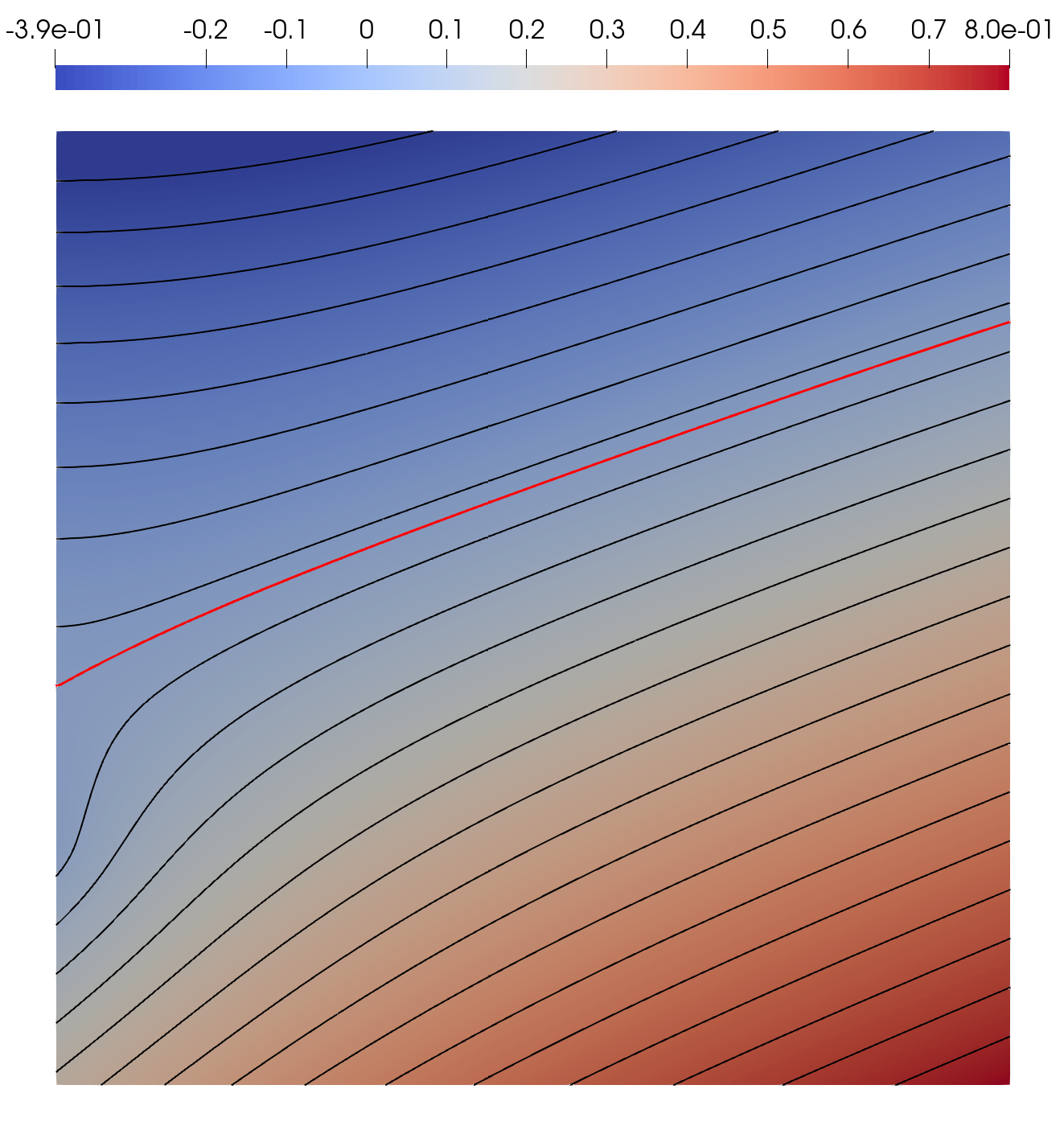
(a) Contours of pressure. Level set $u_{h}=0$ marked with red line.

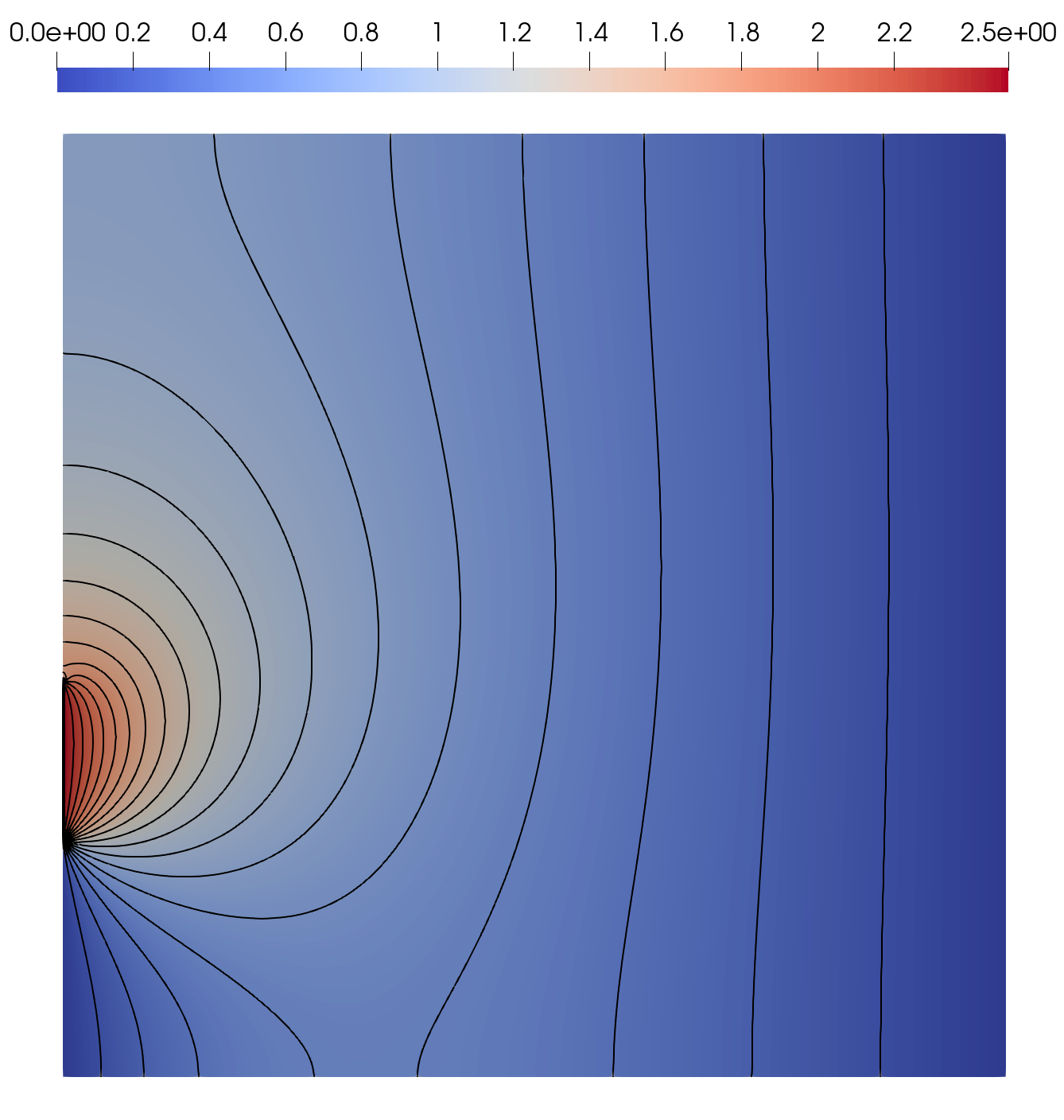
(b) Contours of adjoint variable, $z_{h}$. Note that by definition $z_{h}\geqslant 0$.

(c) $\mathcal{T}^{1}$

(d) $\mathcal{T}^{4}$

(e) $\mathcal{T}^{7}$

(f) $\mathcal{T}^{11}$

Figure 3: Example 1, flow through a single layered, silty soil. We show the pressure, adjoint solution and a sample of adaptively generated meshes showing refinement upstream of the seepage face. The primal variable $u_{h}$ and the adjoint variable $z_{h}$ are both represented on $\mathcal{T}^{11}$ which has approximately 66000 degrees of freedom.

6.2 Example 2: Sloping Unconfined Aquifer with Impeding Layer

Figure 4: The domain models a slope lying on a layer of bedrock with a downstream external boundary. The domain is a parallelogram with corners $(0,1)$, $(0,2)$, $(10,1)$ and $(10,0)$ where all dimensions are in metres. The lower extent of the domain represents an impermeable boundary, as does a layer of rock parallel to the land surface towards the right hand side of the domain. This layer is 0.1m thick with corners $(5,0.95)$, $(5,1.05)$, $(10,0.45)$ and $(10,0.55)$. The water table is fixed with a Dirichlet boundary condition on the left hand boundary of the domain.

The second test case is taken from [26]. Its relevance was shown in [6] where the location of impeding layers was shown to have large effects on the saturation conditions of the soil. The domain setup is illustrated in Figure 4. This configuration leads to water flowing down the slope due to gravity, and allows multiple seepage faces to form. We introduce a forcing term, representing an underground spring, above the layer to force extra seepage faces. It is defined by:

$$f(x)=\begin{cases}10&\text{ if dist($x,(9,1.15))<0.2$}\\ 0&\text{ otherwise.}\end{cases}$$ (55)

We make the same choice of soil parameters as in example 1, that is $n=2.06$, $\alpha=1m^{-1}$, $K_{S}=1{ms^{-1}}$.

The results of this are given in Figure 5. As can be seen in Figure 5(a), three disjoint seepage faces arise from this simulation, two on the right hand face, one above and one below the impermeable barrier, and another at the land surface. It should be noted that the seepage face at the land surface would generate surface run-off. This process is not taken into account by the model we use.

The simulation is initialised on a coarse mesh of 4036 elements. An adaptive simulation using the dual-weighted estimate produced the meshes in figure 5. The algorithm refines heavily around the source and all seepage faces, as well as resolving the corners around the impeding layer.

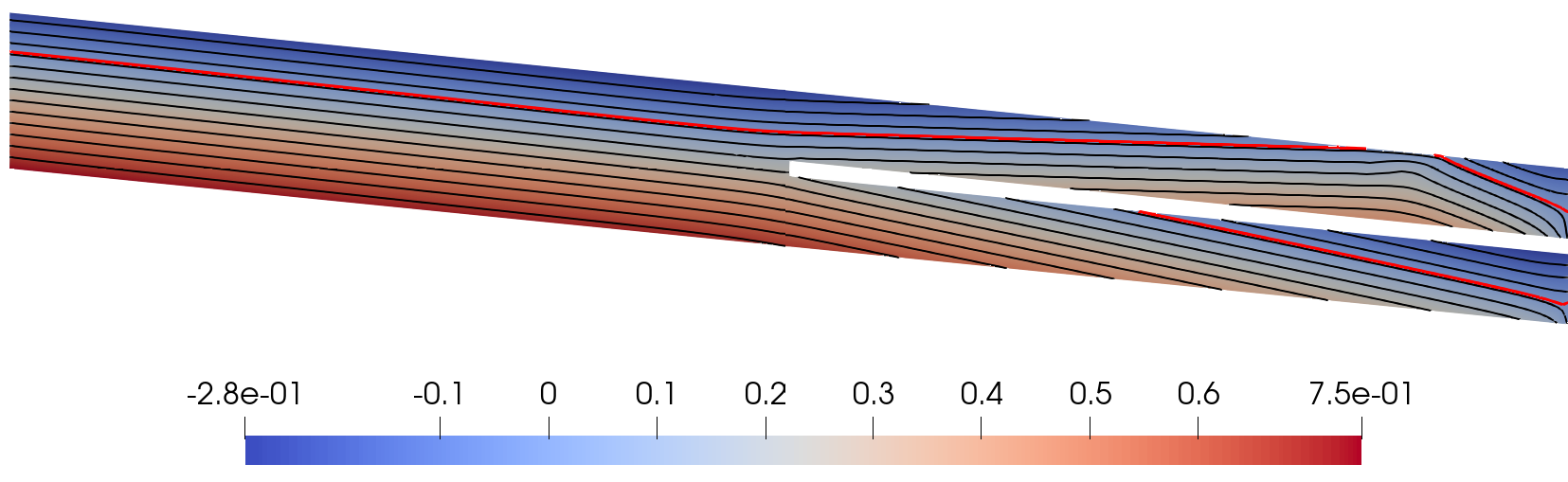
(a) Simulation of hillside with water leak. Level set $u_{h}=0$ marked with red line.

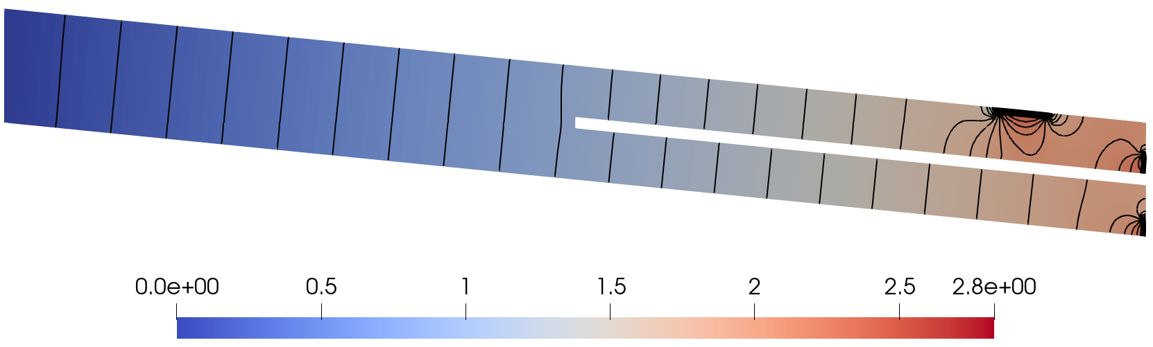
(b) Contours of adjoint variable, $z_{h}$. Note the extreme clustering of contours around the three seepage faces as well as high density around the source.

(c) $\mathcal{T}^{7}$

(d) $\mathcal{T}^{10}$

(e) $\mathcal{T}^{14}$

(f) $\mathcal{T}^{17}$

Figure 5: Example 2, flow through a sloped aquifer with impeding layer. We show the pressure, adjoint solution and a sample of adaptively refined meshes that capture multiple seepage faces as well as potential singularities in the pressure at the corner in the domain. The primal and adjoint variable are both represented on $\mathcal{T}^{17}$ which has approximately $7\times 10^{5}$ degrees of freedom.

6.3 Estimator Effectivity Summary

In Examples 1 and 2 above we compute a reference value for $J(u)$ obtained from a simulation on a very fine grid. This was taken as the ‘true’ value to perform analysis of the behaviour of the estimate. In Figures 6(a)–6(b), we see that as the simulation progresses the effectivity of the estimate, defined as the ratio of the error to the estimate, becomes very close to 1.

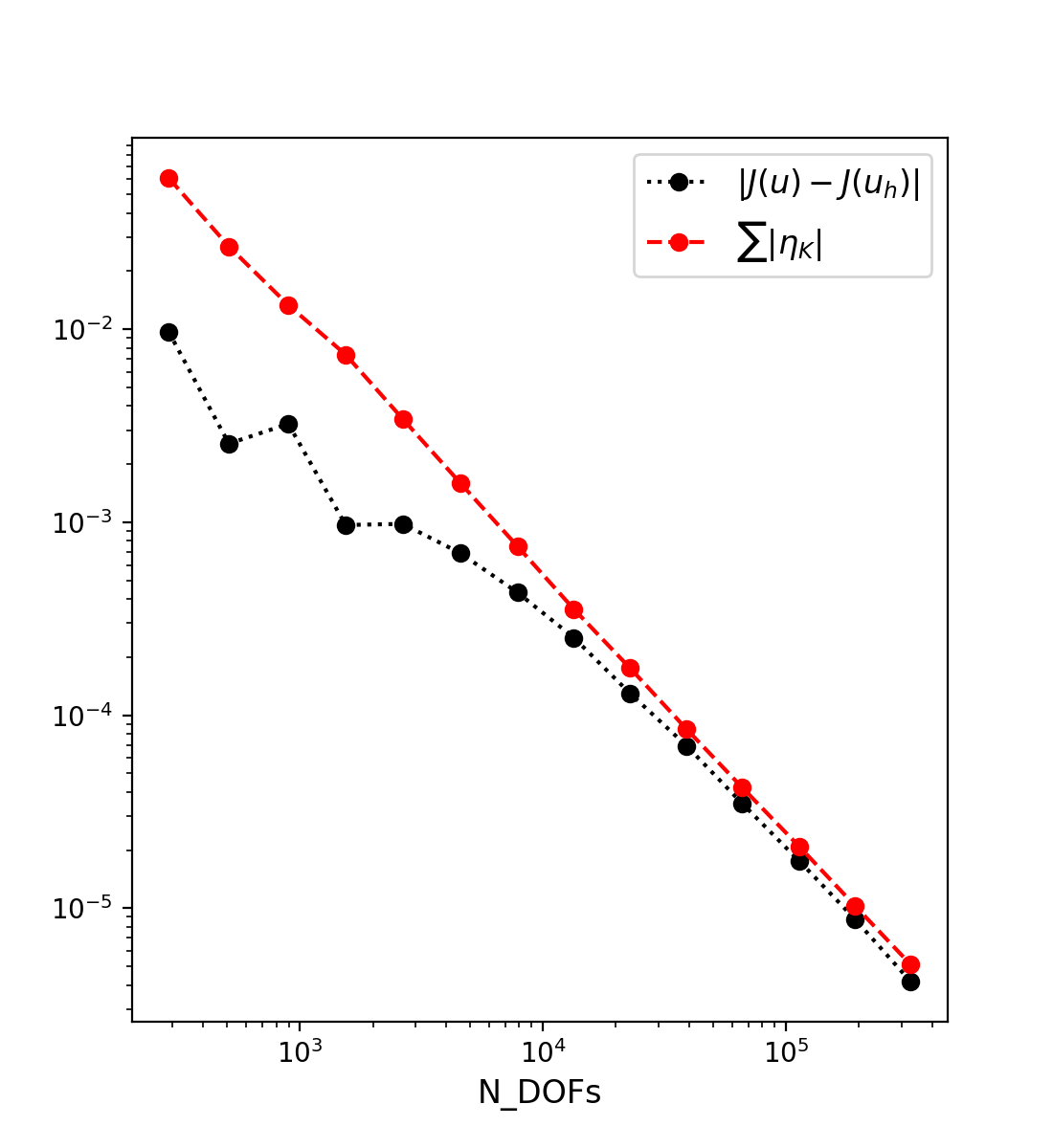
(a) Example 1.

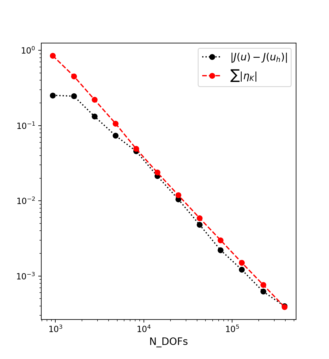
(b) Example 2.

Figure 6: Sharpness of error estimates during adaptive mesh refinement. Notice that the dual-weighted estimate significantly under-estimates the error for the first few refinement cycles but as the simulation progresses the effectivity moves closer to one. This is a well known feature of this class of algorithm further described in [35]

6.4 Adaptive vs Uniform Comparison

To illustrate the gains obtained through adaptive refinement, we make a comparison between the a uniformly refined simulation and the adaptive one. In each case uniform meshes perform extremely poorly with small and unpredictable reductions in error where the adaptive scheme produces fast and monotonic error reduction on all but the coarsest meshes. For comparison, two lines illustrating different rates are included in figure 7(a) illustrating that convergence of $J(u_{h})$ is suboptimal for uniform meshes, and that in terms of degrees of freedom, this optimality can be restored using the goal-based estimate.

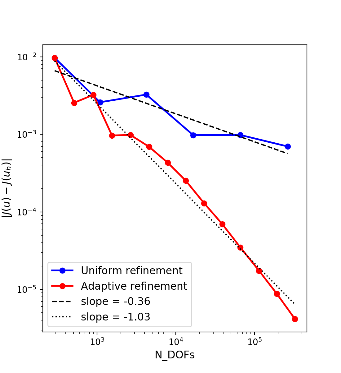
(a) Example 1.

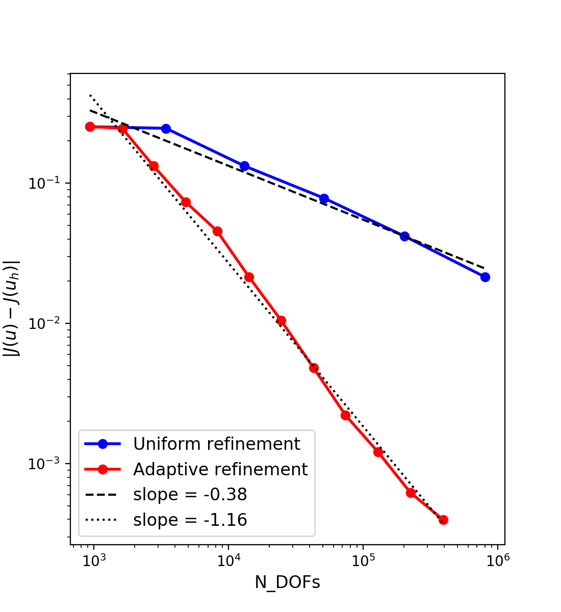
(b) Example 2.

Figure 7: Comparison of orders of convergence in terms of number of degrees of freedom ($N_{DOFS}$) on uniform and adaptive grids. Notice the rate of error reduction is considerably slower for uniform simulations in all cases.

7 Case Studies with Layered Inhomogeneities

We present results making use of borehole data provided by CPRM (Brazilian Geological Survey) by the Siagas system . The wells are used to supply water to two different cities in São Paulo State, Brazil, one in Ibirá and the other in Porto Ferrreira. Both cities are located over the Paraná Sedimentary Basin, but in places with different shallow geology. There are two different problem setups that we consider. In both cases the domain is a vertical section illustrated in Figure 8. We assumed the soil is in homogeneous layers, where there is no variation in the physical properties in the horizontal direction. The soil parameters used for the simulation are given in Table 1. The water table height far from the well is known and applied as a Dirichlet boundary condition for the pressure on the right hand lateral boundary. In both cases, the height of the water in the well gives the left lateral boundary condition, and water is continually pumped out of the well in such a way that the water height remains constant.

We work in cylindrical coordinates with the $(r,\phi,z)$ with the $z$-axis aligned with the centre of the well. The aim is to calculate the total flux into the well. We therefore use the functional $J_{2}$ to account for flux of water over the inner boundary below the water level, defined as follows.

$$J_{2}(u):=2\pi r_{0}\int_{r=r_{0}}\mathbf{q(u)}\cdot\mathbf{n}\mathop{}\!\mathrm{d}z,$$ (56)

where $r_{0}$ denotes the radius of the well, that is, we integrate over the entire inner wall of the well, above and below the water.

(a) Case study 1, well within a two layered soil.

(b) Case study 2, well within a five layered soil.

Figure 8: Geometric setup of the industrial case study problems. Black shading represents an impermeable boundary. In case study two, the gaps between impermeable regions on the inner wall of the well are the filter locations. The far field boundary conditions are analogous to those given in Figure 1 and water is continually pumped out to maintain constant water height.

7.1 Case Study 1 - 2 layered well in Ibirá (CPRM reference 3500023601)

For these case studies, all lengths are given in metres. In the first case we set $\Omega=\{(r,\phi,z)\mid 0.0762\leqslant r\leqslant 50,\,0\leqslant z\leqslant 60\}$. The medium consists of sandy loam for $38\leqslant z\leqslant 60$ and fine sandstone for $0\leqslant z\leqslant 38$. We refer to Table 1 for details of the parametrisations of these soils. Again, the base of the well is assumed to consist of impervious rock, and a no-flow boundary condition is enforced. There is assumed to be no water flow at the land surface. The water table has been measured in the vicinity of the well to be 49.8$m$, so we set a hydrostatic boundary condition at $r=50$ to represent the far field conditions around the well. The height of water in the well is 42.7$m$. The initial mesh is aligned with the layers in the soil. The solution, together with a selection of adaptive meshes are given in Figure 9. The computed flux as a function of degrees of freedom is given in Figure 11(a) showing that the mathematical model is in good agreement with the experimental data.

Table 1: Case study soil parameters. Parameters used in the van Genuchten-Mualem model for hydraulic conductivity in each of the several types of soil and rock. Note the differences of several orders of magnitude in the parameters $K_{S}^{i}$, causing strong discontinuities in the coefficient $k$.

Layer	$K_{S}$ ($ms^{-1}$)	$n$	$\alpha$ ($m^{-1}$)
sandy loam	5E-6	1.65	0.66
med. sandstone	9E-6	1.36	0.012
slate	5.0E-9	6.75	0.98
fine sandstone	1.15E-6	1.361	0.012
diabase	2E-5	1.523	1.066

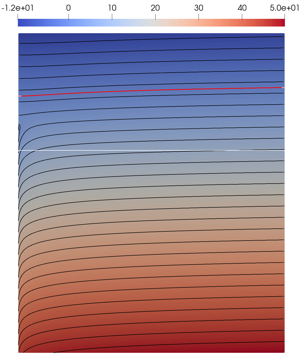
(a) Contours of pressure.

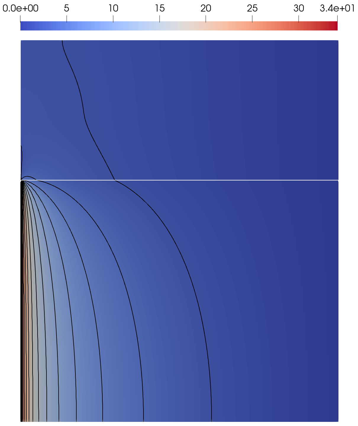
(b) Contours of adjoint pressure, $z_{h}$.

(c) $\mathcal{T}^{15}$

(d) $\mathcal{T}^{20}$

(e) $\mathcal{T}^{30}$

(f) $\mathcal{T}^{35}$

Figure 9: Case study 1, flow through a two layered soil. We show the pressure, the adjoint solution and a sample of adaptively generated meshes. The boundary between the soil layers is marked with a white line. Both solutions are represented on $\mathcal{T}^{35}$ which has approximately 1.5 million degrees of freedom.

7.2 Case study 2 - 5 layered well in Porto Ferreira (CPRM reference 3500009747)

The second case study is a challenging setup with five layers of highly varying hydraulic properties, as well as complex boundary conditions due to the fact that in this case the inner wall of the well is impermeable apart from two filters to allow water to flow into the well. One is below and one above the water, meaning that the former allows flow into the subsurface and the other allows flow out. Along the inner wall, filters cover the part of the wall with $5\leqslant z\leqslant 17$ and $19\leqslant z\leqslant 23$. The water level in the well is set at 17.44, with the other boundary conditions as in case study 1, with the water table at the far boundary set at 33.9. Once again we assume a radially symmetric solution. The domain is given by $\Omega=\{(r,\phi,z)\mid 0.1585\leqslant r\leqslant 50,\,0\leqslant z\leqslant 46\}$. The medium consists of five layers. In order, with the top layer first, the layers consist of sandy loam, medium sandstone, slate, coarse sandstone and diabase. The boundaries between the layers are at $z=34$, $z=18$, $z=16$ and $z=8$. We refer to Figure 8 for a visual description. The slate layer in particular causes this to be a difficult problem to simulate numerically due to its hydraulic conductivity being several of orders of magnitude smaller than those of the other soils and rocks. The initial mesh is aligned with the layers as well as the filter locations and the water level in the well. The solution, together with a selection of adaptive meshes are given in Figure 10. The computed flux as a function of degrees of freedom is given in Figure 11(b) showing a comparison between the mathematical model and the experimental data.

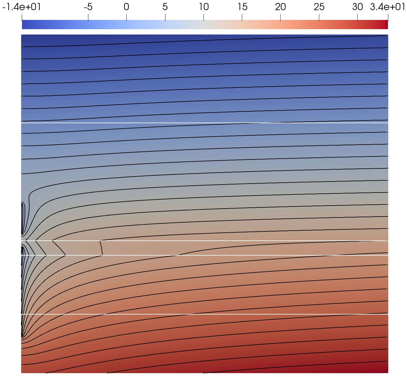
(a) Contours of pressure.

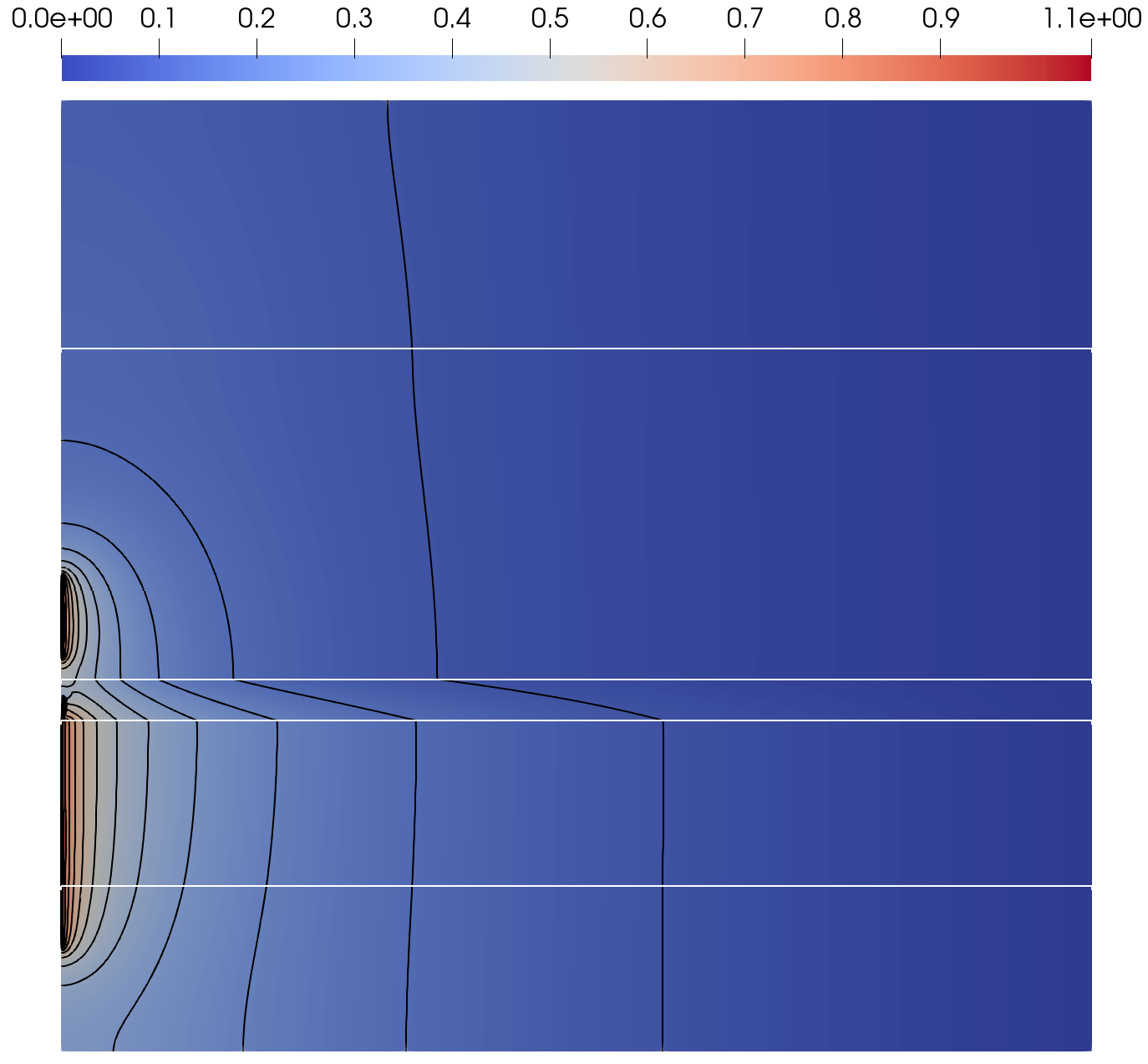
(b) Contours of adjoint pressure, $z_{h}$.

(c) $\mathcal{T}^{20}$

(d) $\mathcal{T}^{25}$

(e) $\mathcal{T}^{35}$

(f) $\mathcal{T}^{45}$

Figure 10: Case study 2, flow through a 5 layer soil. Level set $u=0$ marked with red line. The boundaries between the soil layers are marked with white lines. See table 1 for a detailed description of the properties of each layer. Both solutions are represented on $\mathcal{T}^{45}$ which has approximately 500,000 degrees of freedom. Note that in this case the dual problem is much more interesting due to the structure of the inner wall of the well. The meshes appear to show that the soil layers have very different influences on solution accuracy. In particular, the slate layer shows little mesh refinement due to its low permeability relative to the other layers.

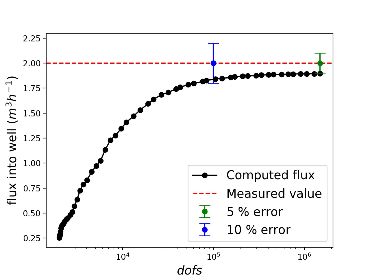
(a) Case study 1. Note that the fully resolved model is within a 5% relative error of the experimental results with a 10% relative error at around $90000$ degrees of freedom.

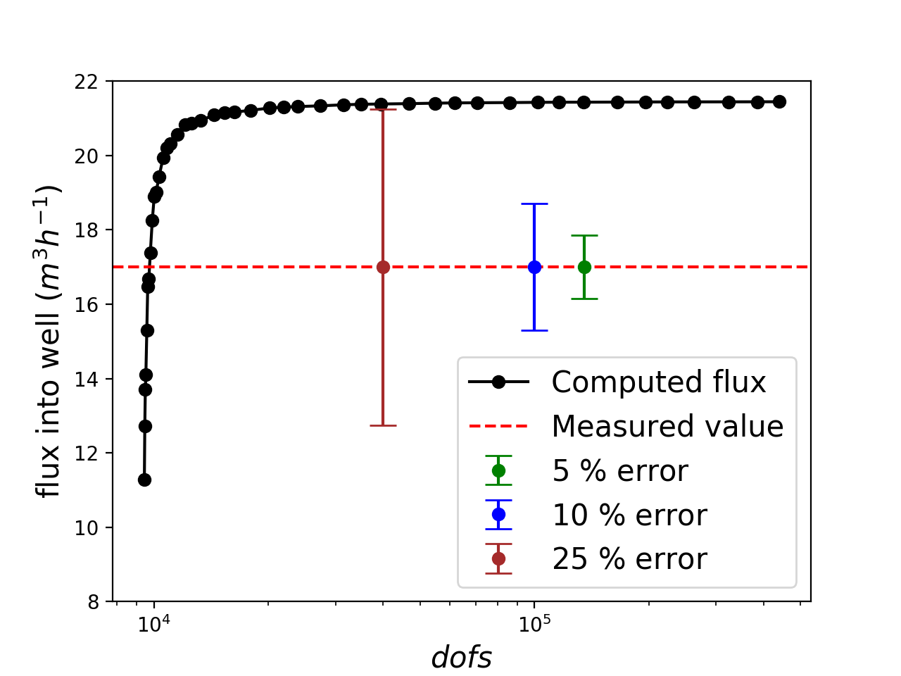
(b) Case study 2. The fully resolved model is around 25% relative error. This is already achieved with $20000$ degrees of freedom. dafuhhadf

Figure 11: Plots displaying the computed value of the water flux into the well under successive refinement cycles of the adaptive finite element method. This allows to infer the maximal amount of water pumped from the well whilst leaving the surrounding water table unchanged.

8 Conclusions & Discussion

In this article, we applied techniques from goal-oriented a posteriori error estimation to a challenging nonlinear problem involving a groundwater flow. For this class of problem, fine uniform meshes do not perform well. Indeed, in Figure 7 we see that convergence can be extremely slow on uniform meshes. By comparison, the dual-weighted error estimate was shown to perform well under a variety of conditions. It has been observed in previous studies (see for example [35]) that due to the approximations that must be made to evaluate the error representation numerically, the error estimate can perform poorly if the initial mesh in simulations is too coarse. In this particular case, we expect that the problem originates in the approximation of the dual problem. Since the dual solution must satisfy homogeneous Dirichlet boundary conditions on the seepage face defined by the primal solution, and since the forcing from the quantity of interest is largest here, there is a sharp boundary layer at the seepage face which is inevitably poorly resolved by a coarse mesh. Notwithstanding, the algorithm produces rapid error reduction with effectivity close to 1 once the mesh is sufficiently locally refined. This means that numerical error can be quantified with a high degree of confidence, and that the dual-weighted error estimate can be used as a termination criterion for an adaptive routine.

The case studies most clearly demonstrate the need for adaptive techniques in solving problems such as this. The multi-scale nature of inhomogeneous soil results in a problem which is extremely challenging to solve by conventional numerical methods. Indeed, the error remains large on uniform meshes even as the mesh approaches $10^{5}$ degrees of freedom where in the adaptive case a steep and consistent reduction in error can be observed with successively refined meshes, see Figure 7. Applying these robust, computationally efficient methods to the case studies allows the accurate quantification of solutions to the variational inequality. Note, however, that these case studies are still extremely challenging. The assumption of layered soil, for example, may not always be physically meaningful. Indeed, we believe it is this assumption that affects the performance of case study 2. For highly variable soils we must use further information, for example those provided through resistivity methods. This is the subject of ongoing research.

References

- [1] E. Milakis and L. Silvestre. Regularity for the nonlinear Signorini problem. Advances in Mathematics, 217(3):1301–1312, 2008.
- [2] M. Darbandi, S.O. Torabi, M. Saadat, Y. Daghighi, and D. Jarrahbashi. A moving-mesh finite-volume method to solve free-surface seepage problem in arbitrary geometries. International Journal for Numerical and Analytical Methods in Geomechanics, 31(14):1609–1629, 2007.
- [3] H. Brezis. Sur une nouvelle formulation du problème de l’écoulement à travers une digue. CR Acad. Sci. Paris, 287:711–714, 1978.
- [4] J. T. Oden and N. Kikuchi. Theory of variational inequalities with applications to problems of flow through porous media. International Journal of Engineering Science, 18(10):1173–1284, 1980.
- [5] J. Zhang, Q. Xu, and Z. Chen. Seepage analysis based on the unified unsaturated soil theory. Mechanics Research Communications, 28(1):107–112, 2001.
- [6] J. J. Rulon, R. Rodway, and R. A. Freeze. The development of multiple seepage faces on layered slopes. Water Resources Research, 21(11):1625–1636, 1985.
- [7] R. S. Falk. Error estimates for the approximation of a class of variational inequalities. Mathematics of Computation, 28(128):963–971, 1974.
- [8] R. Hartmann and P. Houston. Adaptive discontinuous Galerkin finite element methods for the compressible euler equations. Journal of Computational Physics, 183(2):508–532, 2002.
- [9] K. A. Cliffe, J. Collis, and P. Houston. Goal-oriented a posteriori error estimation for the travel time functional in porous media flows. SIAM Journal on Scientific Computing, 37(2):B127–B152, 2015.
- [10] H. Blum and F.-T. Suttmeier. An adaptive finite element discretisation for a simplified Signorini problem. Calcolo, 37(2):65–77, 2000.
- [11] F.-T. Suttmeier. Numerical solution of variational inequalities by adaptive finite elements. Springer, 2008.
- [12] G. Şimşek, X. Wu, K.G. van der Zee, and E.H. van Brummelen. Duality-based two-level error estimation for time-dependent PDEs: Application to linear and nonlinear parabolic equations. Computer Methods in Applied Mechanics and Engineering, 288:83–109, 2015.
- [13] W. Bangerth and R. Rannacher. Finite element approximation of the acoustic wave equation: Error control and mesh adaptation. East West Journal of Numerical Mathematics, 7(4):263–282, 1999.
- [14] M. Van Genuchten. A closed-form equation for predicting the hydraulic conductivity of unsaturated soils. Soil Sci. Soc. Am. J., 44:892–898, 1980.
- [15] E. Buckingham. Studies on the movement of soil moisture. US Dept. Agic. Bur. Soils Bull., 38:28–36, 1907.
- [16] J. Bear. Dynamics of fluids in porous media. Dover, 1988.
- [17] J.-L. Lions and G. Stampacchia. Variational inequalities. Communications on pure and applied mathematics, 20(3):493–519, 1967.
- [18] D. Kinderlehrer and G. Stampacchia. An introduction to variational inequalities and their applications, volume 31. SIAM, 1980.
- [19] M. Bause and P. Knabner. Computation of variably saturated subsurface flow by adaptive mixed hybrid finite element methods. Advances in Water Resources, 27(6):565 – 581, 2004.
- [20] Philippe G Ciarlet. The finite element method for elliptic problems. SIAM, 2002.
- [21] C. Christof and C. Haubner. Finite element error estimates in non-energy norms for the two-dimensional scalar Signorini problem. Preprint IGDK-2018-14, IGDK, 2020.
- [22] R. Becker and R. Rannacher. An optimal control approach to a posteriori error estimation in finite element methods. Acta numerica, 10:1–102, 2001.
- [23] Y. Mualem. A new model for predicting the hydraulic conductivity of unsaturated porous media. Water resources research, 12(3):513–522, 1976.
- [24] M. Van Genuchten and D.R. Nielsen. On describing and predicting the hydraulic properties. Annales Geophysicae, 3(5):615–628, 1985.
- [25] C. Paniconi and M. Putti. A comparison of Picard and Newton iteration in the numerical solution of multidimensional variably saturated flow problems. Water Resources Research, 30(12):3357–3374, 1994.
- [26] C. Scudeler, C. Paniconi, D. Pasetto, and M. Putti. Examination of the seepage face boundary condition in subsurface and coupled surface/subsurface hydrological models. Water Resources Research, 53(3):1799–1819, 2017.
- [27] S. P. Neuman. Saturated-unsaturated seepage by finite elements. Journal of the Hydraulics Division., PROC., ASCE., pages 2233–2250, 1973.
- [28] R. L. Cooley. Some new procedures for numerical solution of variably saturated flow problems. Water Resources Research, 19(5):1271–1285, 1983.
- [29] W. Dörfler. A convergent adaptive algorithm for Poisson’s equation. SIAM J. Numer. Anal., 33(3):1106–1124, 1996.
- [30] D. Arndt, W. Bangerth, T. C. Clevenger, D. Davydov, M. Fehling, D. Garcia-Sanchez, G. Harper, T. Heister, L. Heltai, M. Kronbichler, R. M. Kynch, M. Maier, J.-P. Pelteret, B. Turcksin, and D. Wells. The deal.II library, version 9.1. Journal of Numerical Mathematics, 2019. accepted.
- [31] W. Bangerth and R. Rannacher. Adaptive finite element methods for differential equations. Birkhäuser, 2013.
- [32] A. Dedner, J. Giesselmann, T. Pryer, and J. K. Ryan. Residual estimates for post-processors in elliptic problems. to appear in Journal of Scientific Computing, 2019.
- [33] M. J. Kazemzadeh-Parsi and F. Daneshmand. Unconfined seepage analysis in earth dams using smoothed fixed grid finite element method. International Journal for Numerical and Analytical Methods in Geomechanics, 36(6):780–797, 2012.
- [34] H. Zheng, D.F. Liu, C.F. Lee, and L.G. Tham. A new formulation of Signorini’s type for seepage problems with free surfaces. International Journal for Numerical Methods in Engineering, 64(1):1–16, 2005.
- [35] R. H. Nochetto, A. Veeser, and M. Verani. A safeguarded dual weighted residual method. IMA Journal of Numerical Analysis, 29(1):126–140, 2008.