Kinematics and Multi Band Period-Luminosity-Metallicity Relation of RR Lyrae Stars via Statistical Parallax

Abstract

This paper presents results from photometric and statistical-parallax analysis of a sample of 850 field RR Lyrae (RRL) variables. The photometric and spectroscopic data for sample RRLs are obtained from (1) our new spectroscopic observations (for 448 RRLs) carried out with the Southern African Large Telescope (SALT); (2) our photometric observations using the 1.0-m telescope of the South African Astronomical Observatory (SAAO), and (3) literature. These are combined with accurate proper motion data from the second release of Gaia mission (DR2). This study primarily determines the velocity distribution of solar neighborhood RRLs, and it also calibrates the zero points of the RRLs visual V-band luminosity-metallicity (LZ or $M_{V}-$[Fe/H]) relation and their period-luminosity-metallicity (PLZ) relations in the WISE $W_{1}-$ and 2MASS $Ks-$band. We find the bulk velocity of the halo RRLs relative to the Sun to be $(U_{0},V_{0},W_{0})_{\text{Halo}}$ $=(-16\pm 7,-219\pm 7,-6\pm 5)$ km s^-1 in the direction of Galactic center, Galactic rotation and North Galactic pole, respectively, with velocity-dispersion ellipsoids $(\sigma V_{R},\sigma V_{\phi},\sigma V_{\theta})_{\text{Halo}}=$ $(153\pm 7,106\pm 4,101\pm 4)$ km s^-1. The corresponding parameters for the disk component are found to be $(U_{0},V_{0},W_{0})_{\text{Disk}}=$ $(-19\pm 5,-46\pm 5,-14\pm 3)$ km s^-1 and $(\sigma V_{R},\sigma V_{\phi},\sigma V_{\theta})_{\text{Disk}}=$ $(49\pm 4,38\pm 4,25\pm 3)$ km s^-1. The calibrated PLZ in $W_{1}-$, $Ks-$band, and V-band LZ relations are $\langle\,M_{W1}\rangle=$ $-0.824+0.124[Fe/H]-2.381\log\,P_{F}$, $\langle M_{Ks}\rangle=$ $-0.804+0.101[Fe/H]-2.33\log\,P_{F}$ and $\langle\,M_{V}\rangle=1.041+0.232[Fe/H]$, respectively. The calibrated PLZ and LZ relations are used to estimate the Galactic Center distance and the distance modulus of the Large Magellanic Cloud (LMC), which are found to be 7.99$\pm$0.49 kpc and 18.46$\pm$0.09  mag, respectively. All our results are in excellent agreement with available literature based on statistical parallax analysis, but are considerably more accurate and precise. Moreover, the zero-points of our calibrated PLZ and LZ relations are quite consistent with current results found by other techniques and yield the LMC distance modulus that is within 0.04 mag of the current most precise estimate.

1 Introduction

RR Lyrae type variables are low mass stars that have evolved off the main sequence when their core hydrogen is exhausted and that occupy a fairly narrow strip in the Hertzsprung-Russell diagram at the intersection of the pulsating-star instability strip and the horizontal branch when their mean effective temperature reach $\sim 6000-7500$ K (Iben Jr, 1974). Thus, they are old low-mass yellow or white giants in the core helium burning stage (Salaris & Cassisi, 2005) and belong to Population II (Smith, 1995; Lipka, 2012). Therefore, they can serve as distance indicators, as well as kinematics and metallicity tracers of old populations (Dambis et al., 2013, and the reference there in). They are radially pulsating A–F type stars which pulsate with periods 0.2-1.2 d (Catelan, 2009). They were once stars with similar or slightly lower mass than the Sun, around 0.8 solar masses (Cacciari, 2012). Most of them are classified into three main types according to the mode in which they pulsate radially: fundamental-mode RRab stars, first-overtone RRc stars and double-mode RRd stars. They are easily identified by their periods and characteristic light-curve shapes. Like other pulsating stars they have their own PLZ relation in any band (Nemec et al., 1994; Catelan et al., 2004).

RRLs can be used as standard candles because of their LZ and PLZ relations. The near- or mid-infrared wavelength (hereafter NIR or MIR) PLZ relations are more preferable than the visual $M_{V}-[Fe/H]$ relation, because they are less dependent on interstellar extinction, metallicity and evolution effects. For example, reddening in the visual V-band is one order of magnitude grater than in the K-band (Cardelli et al., 1989, $A_{K}=0.114A_{V}$), and it is roughly 15 times stronger than in the W1-band (Madore et al., 2013, $A_{W1}=0.065A_{V}$). Moreover, the mean magnitudes of RRLs in NIR- and MIR-bands can be estimated more accurately than their mean visual V-band magnitudes due to the smaller amplitude of infrared light curves (Jones et al., 1996; Monson et al., 2017). Despite these useful features of PLZ and LZ relations, there is still no agreement about their parameters especially concerning the zero points. One of the problems is the persistent tension between the results coming from the statistical parallax methods with those from other techniques (pulsational models, Baade-Wesselnik, eclipsing binaries, RGB tip, etc.). We therefore try to recalibrate the zero points of visual V -band LZ and Ks- and W1-band PLZ relations of RRLs by applying the maximum likelihood version of statistical parallax technique to a sample with more than twice the size of the largest such list employed so far.

Statistical parallax is a primary method that can determine simultaneously both the distance scaling parameter (the mean absolute magnitude) and velocity ellipsoid parameters (like the bulk velocity and velocity dispersion) of a set of stars from observables including proper motions and radial velocities. Historically, statistical-parallax analysis of RRL stars was originally used by Pavlovskaya (1953) and later was the subject of study by many different authors (e.g. Rigal, 1958; Herk et al., 1965; Hemenway, 1975; Hawley et al., 1986; Strugnell et al., 1986; Layden et al., 1996; Tsujimoto et al., 1997; Fernley et al., 1998; Gould & Popowski, 1998; Luri et al., 1998; Popowski & Gould, 1998; Clube & Dawe, 1980; Kollmeier et al., 2013; Dambis & Rastorguev, 2001; Dambis, 2009; Dambis et al., 2013; Dambis et al., 2014; Dambis et al., 2017). It is difficult to show exactly how these different authors use the method independently, since they share a common developmental history and employ similar kinematic modeling procedures — except a few earlier studies all authors use what is known as the maximum likelihood method. However, these studies do show clear differences in such details as the sample size used, the numerical techniques used to maximize the likelihood function, the way in estimating the uncertainties of the derived parameters, with some authors incorporating additional features such as Herk et al. (1965) using automatic rejection of outliers and Luri et al. (1996) considering the case of a multicomponent population (Layden, 1998).

Popowski & Gould (1998) investigated how the size of the sample, observational errors, systematic errors and other potential biases affect the statistical parallax solution by deriving analytic expressions for the uncertainties of each inferred parameter. According to their study, the error of statistical parallax solution parameters, like the distance scaling factor, generally behave as $\varpropto N^{-\frac{1}{2}}\kappa^{-1}$; where N is sample size, $\kappa=W/\sigma$ is the ‘Mach number’ which depends on bulk velocity (W) and velocity dispersion ($\sigma$). They also verified that the systematic errors for the solutions are generally small and these can be corrected using Monte Carlo simulations. Therefore, the accuracy of statistical parallax solution parameters improves as the sample of stars with accurate proper motions and radial velocities is increased in size.

Hence building a large enough sample of RR Lyrae type variables with precise and homogeneous photometry, metallicity, proper motion and bona fide radial velocities is of prime importance for performing statistical parallax. Despite this fact, only about 400 plus RRLs in the extended solar neighborhood had all these data available (Dambis et al., 2013) until recently. To alleviate this we carried out the MAGIC project (see Kniazev et al., 2019, for brief description of the project) with SALT (Buckley et al., 2006; O’Donoghue et al., 2006) telescope with the purpose of acquiring the observationally expensive spectroscopic data for the greatest possible number of RRLs in addition to our long-term program of photometric observations of these variables (Dambis et al., 2017). Thus, our new radial velocity and metallicity data for 448 RRLs coming from this program as will be published by A.Y.Kniazev (in preparation) bring the size of the sample to 850 stars.

Furthermore, Gaia DR2 has recently published multi-band photometry (Gaia G, $\textit{G}_{BP}$ and $\textit{G}_{RP}$ ) data as well as five-parameter astrometric (position, parallax, and proper motion) solutions for $\approx$1.3 billion sources as calculated solely from Gaia astrometry (Gaia Collaboration et al., 2018b). For the sources with five-parameter Gaia astrometric solutions the median uncertainty in parallax at the reference epoch J2015.5 is about 0.04 mas for bright (G < 14 mag) sources, 0.1 mas at G = 17 mag, and 0.7 mas at G = 20 mag, and the corresponding uncertainties in the proper motion components are 0.05, 0.2, and 1.2 mas $\text{yr}^{-1}$, respectively (Lindegren et al., 2018). Furthermore, Gaia proper motion data are more uniform and accurate than previously published catalogs. Therefore, it is now an opportune time for a new statistical parallax analysis in order to use the benefit of our more extensive spectroscopic data combined with high quality Gaia proper motion data.

In this study we estimate the velocity distribution of Galactic field RRLs in the solar neighborhood, and refine the zero point of the $M_{V}-[Fe/H]$ and PLZ relations in the WISE W1- and 2MASS Ks-bands via statistical parallax technique. We also use multiband photometric data and estimates obtained from a fide 3D interstellar extinction model (Drimmel et al., 2003) to calibrate RRL $(V-Ks)_{0}$ and $(V-W_{1})_{0}$ intrinsic colours in terms of fundamental period and metallicity by following the footsteps of Dambis et al. (2013). The improvement in this study includes addition of our own new photometric and spectroscopic data for about 448 RRLs, which is 111 % increase over the largest such sample studied so far combined with accurate Gaia proper motion data.

This paper is organized as follows. Section 2 describes in detail the data used in our statistical parallax analysis and how it is compiled. Section 3 reminds the basic principles and provides an overview of statistical parallax technique. Section 4 provides the main results of this work: the kinematic model of Galactic field RRLs; calibrated LZ and PLZ relations of RRLs, and discusses the implication of our results to determine Gaia DR2 parallax offset, Galactic center distance and LMC distance modulus. Finally, we summarize our conclusions in Section  5.

2 Data

As we stated in our previous section, in order to determine the kinematic model parameters and calibrate the $M_{V}-[Fe/H]$ and PLZ relations in the $Ks$- and $W_{1}$-bands using statistical parallax method with better precision, we need a large sample of RRLs with accurate and precise (1) apparent mean magnitude in the Johnson V, 2MASS Ks and WISE $W_{1}$ pass-bands; (2) known periods and pulsation modes; (3) metallicities, proper motions, radial velocities and extinctions in one of the pass-bands. Initially, our sample for this work consists of 850 RRLs. Depending on the spectroscopic data source, we subdivide this sample of RRLs into two parts: The first one is the most complete sample of Galactic field RRL type variables employed in our previous statistical parallax analysis (Dambis et al., 2013), this list initially includes a total of 403 Galactic field RRL stars but one RRL is discarded due to current updates (see Sect 2.1); the second part consists of 448 RRL type variables, which have our own new spectroscopic data acquired as a result of observations performed with SALT telescope. The next subsections describe each type of data in detail.

2.1 Periods and pulsation modes

The accuracy of the phased data relies on the accuracy of the pulsation periods. Thus, the periods and pulsation modes of the first part of the RRLs samples used in this work were adopted from our previous study (Dambis et al., 2013), at that time we took these pulsation periods from ASAS3 catalogue (Pojmanski, 2002), Maintz (2005) compilation and General Catalogue of Variable Stars (GCVS, Samus et al., 2012). However, recently GCVS (Samus et al., 2017) updated parameter values for some RRLs in this sample. Following these updates, we adopt different period values than in our previous study for 28 RRLs (in the range from the longest SS Gru to shortest DI Aps periods), and the pulsation mode of DH Peg and EZ Cep were changed to RRC and RRAB, respectively. Moreover, BI Tel (P=1.17 days) turned out to be an Anomalous Cepheid and was hence discarded (Muraveva et al., 2018a). Our final sample from this group consists of 402 RRLs, of which 367 pulsate in the fundamental mode and 35 in the first overtone mode.

Given that some RRLs show short time scale random period fluctuations, it is unsafe to use outdated published ephemerides to calculate the phases of our SALT spectroscopic observations (e.g. Berdnikov et al., 2017). We therefore determined the periods and pulsation modes for the stars of the second part of our RRL sample from the time series analysis of our own photometric observations obtained with the 1-m telescopes of SAAO in 2016 as well as the data from recently published All-Sky Automated Survey for Supernovae (ASAS-SN) catalogue (Kochanek et al., 2017) with epochs close to our SALT spectroscopic observations (see the next section for details).

The fundamental-mode periods ($P_{F}$) for first-overtone pulsators (99 RRc type variables) of our total sample were computed as $\log P_{F}=\log P+0.127$ (Iben Jr, 1974). Figure 1 shows the distribution of fundamental periods for our total sample, with the shortest period being P=0.25 days (DI Aps) and the longest P=0.96 days (SS Gru). Thus our sample spans a representative range of RRL periods and contains both RRab and RRc type stars.

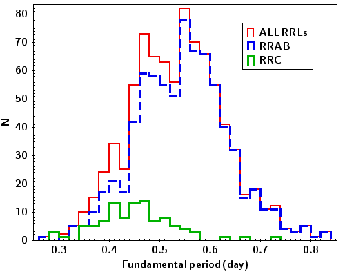
Figure 1: The distribution of fundamental periods.

2.2 Apparent intensity-mean magnitudes in the V-, Ks- and W1-bands

Like the case of the period, we initially adopt the apparent intensity-mean magnitudes for the first group of 402 RRL samples in the Johnson V, 2MASS $K_{s}$ and WISE W1 passbands from Dambis et al. (2013) publication, and then update some of these values based on the resent literatures. According to that paper, (1) the V-band intensity-averaged magnitudes were calculated from nine overlapping sets of observations (see Dambis et al., 2013, and references therein for details); (2) the Ks-band intensity-averaged magnitudes for most of stars were estimated by applying Feast et al. (2008) phase correction procedure on their single-epoch Ks measurements of 2MASS (Cutri et al., 2003); (3) the single-epoch 2MASS Ks magnitudes without phase-corrections were adopted for 32 RRLs, which did not have ephemeris or it was too outdated; (4) the Ks-band intensity-averaged magnitude for thirty stars were adopted from Kinman et al. (2007, 2012), and (5) the W1-band intensity-averaged magnitudes for 398 RRL samples were computed (via Fourier fit) from the WISE All-Sky data release (Cutri et al., 2012).

For the sake of clarity, the compilation of multi-wavelength (V, Ks, W1) mean magnitudes for our total sample using our observations and archives data are presented in the following subsections as organized by passband. Optical-, MIR- and NIR-band data are described in Subsection 2.2.1, Subsection 2.2.2 and Subsection 2.2.3, respectively.

2.2.1 V-band data

As we already pointed out, in order to complement our spectroscopic observations for the second part of our sample, we analyzed the photometry data obtained from our observations and ASAS-SN in order to determine the pulsation characteristics (period, epoch of maximum light, amplitudes and mean magnitudes) of the corresponding RRLs.

Our photometric observations and Data Reduction

We had performed photometric observations for a subset of 197 stars that belongs to the second part of our sample during two observing runs between March and May 2016 using 1-m telescope of SAAO equipped with $BVI_{c}$ filters of the Kron-Cousins system (Cousins, 1976). During photometric nights we were observing two pairs of extinction stars or standard stars (one red and one blue: one pair near the zenith and the other near an air mass of two) in every two to three hours interval (according to the routine described in Berdnikov et al., 2012, and the references therein), in addition to visible target RRLs. We use these observations to calculate the extra atmospheric magnitudes of extinction stars by determining the atmospheric extinction coefficients. We use the same measurements of these standard stars to derive the transformation coefficients and zero points, which helps us to transform the instrumental extra atmospheric magnitudes to the standard Kron-Cousins $BVI_{c}$ system.

We therefore used the same reduction routines as those employed in Berdnikov et al. (2012) to initially reduce the CCD frames taken on all photometric night only. These would let us to determine seasonal mean transformation coefficients which would then be applied to observations of the same standards on each night in order to find the zero points for each night. We thus compiled a catalog of positions and magnitudes of all objects on the best CCD frames from the reduction for all photometric nights. We then selected constant stars from this catalog and used them as comparison stars for differential photometry of all stars on all CCD frames including those taken on non-photometric nights. All this is done by using our own reduction package (custom software developed by L.Berdinkov).

Our BV$I_{c}$ measurements for a typical example RT Ant are presented in Table 1, and the corresponding phased light curve is shown in Fig. 2. The accuracy of our individual observations is nearly 0.01 mag in all filters. Our measured data for 197 RRLs subsample (as illustrated in Fig. 2) are generally not sufficient to model their light curves accurately. For this reason we complemented the time series analysis of our measured V-band observations with ASAS-SN data and applied the Lomb-Scargle Algorithm (Barning, 1963; Lomb, 1976; Scargle, 1982) to determine the initial ephemerides. We then used these ephemerides to determine the amplitudes, intensity mean magnitudes (with uncertainties in the order of $\pm 0.01$ mag) and epochs of maximum light via the Hertzsprung (1919) method employing the algorithm proposed by Berdnikov (1992). Additional light curve data and plots for 33 and 163 of the samples using our observations had been published in Dagne et al. (2017) and Muhie et al. (2020), respectively (available in their online version).

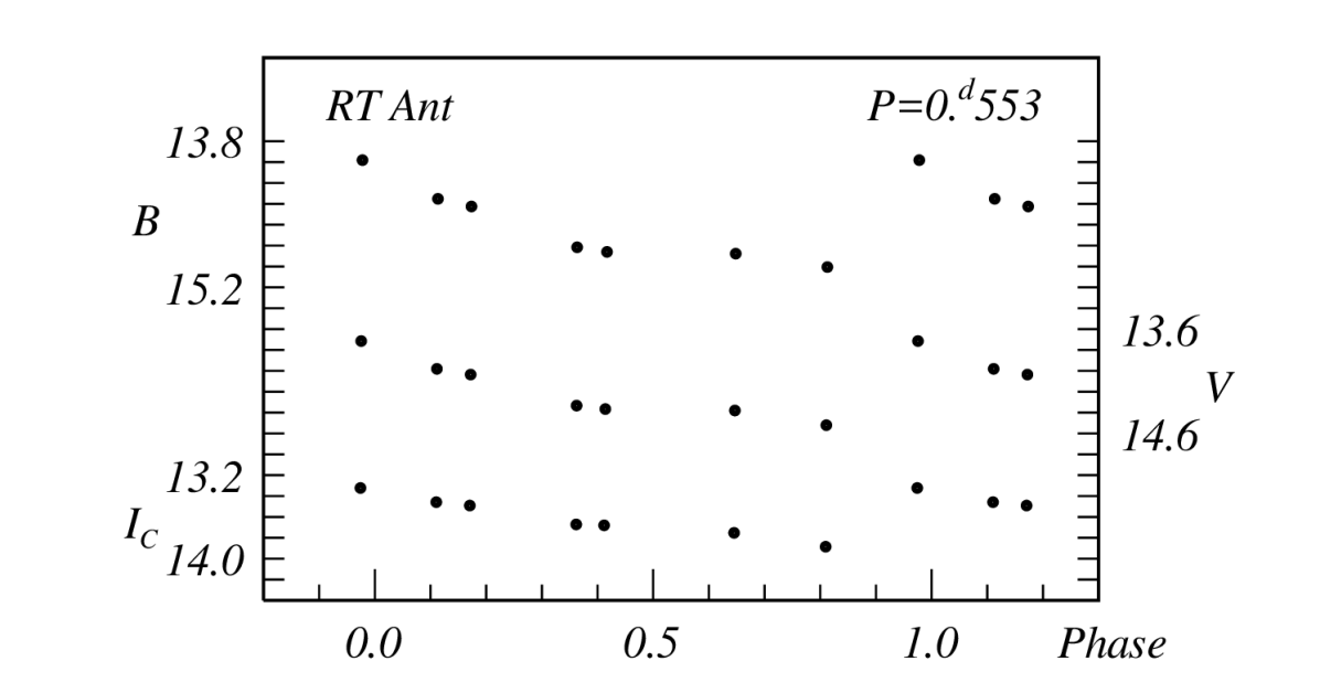
Figure 2: Phased light curve of RT Ant.

Table 1: Photometric Observations of RT Ant

HJD 2400000	Filter	Magnitude	HJD 2400000	Filter	Magnitude	HJD 2400000	Filter	Magnitude
57467.4702	$I_{c}$	13.885	57467.4708	$V$	14.521	57467.4719	$B$	15.006
57469.4620	$I_{c}$	13.680	57469.4632	$V$	14.366	57469.4648	$B$	14.860
57470.4345	$I_{c}$	13.491	57470.4353	$V$	14.036	57470.4361	$B$	14.425
57473.4618	$I_{c}$	13.752	57473.4625	$V$	14.380	57473.4634	$B$	14.877
57476.4837	$I_{c}$	13.458	57476.4843	$V$	13.981	57476.4854	$B$	14.352
57479.3875	$I_{c}$	13.672	57479.3878	$V$	14.333	57479.3884	$B$	14.816
57480.2791	$I_{c}$	13.323	57480.2799	$V$	13.715	57480.2812	$B$	13.981

ASAS-SN

The ASAS-SN project is working towards imaging the entire visible sky every night to a depth of V $\sim$ 17 mag; its aperture photometry data with $\sim 100-400$ epochs of observation that spans $\sim 2-5$ years up to now are freely accessible at ASAS-SN website (Kochanek et al., 2017). Thus, compared to other surveys which have photometry from one to more than ten years older than our SALT spectra measurement, ASAS-SN data can give us pulsation parameters near the dates of our SALT spectroscopic measurements. We therefore used the ASAS-SN V-band data with epochs close enough to our SALT spectroscopy measurements to determine the phases of these measurements.

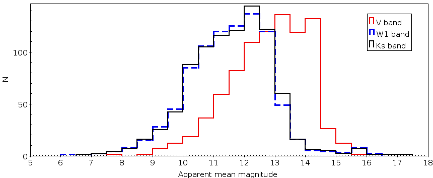
Figure 3: Apparent magnitudes distribution.

Note, however, that ASAS-SN data, which proved to be invaluable for determining the accurate phases of spectroscopic observations, may yield not sufficiently accurate intensity-mean magnitudes because of the large pixel size ($\sim$ 8 arcsec). On the other hand, Gaia DR2 provides photometry in three bands ($G$, $B_{P}$, and $R_{P}$) based on about one dozen-plus visits. We used the homogenized $V$-band intensity-mean magnitudes from (Dambis et al., 2013) combined with the intensity-mean magnitudes derived from our new CCD observations to calibrate $<V>$ in terms of the average $B_{P}$, and $R_{P}$ magnitudes provided in Gaia DR2:

$$<V>=B_{P}+(0.146~{}\pm~{}0.047)-(0.763~{}\pm~{}0.112)(B_{P}-R_{P})$$ (1)

$$+(0.268~{}\pm~{}0.063)(B_{P}-R_{P})^{2}$$

with a scatter of 0.109. The scatter is substantially smaller than the 3-$\sigma$-clipped standard deviation of the difference between the intensity-mean magnitudes inferred from ASAS-SN data and the estimates derived via equation (1), which is equal to $\sim$ 0.17, and we therefore adopt the intensity-mean $V$-band magnitudes converted from Gaia DR2 photometry for 251 stars lacking in our earlier list and without our CCD observations (including 19 stars from (Dambis et al., 2013) with no V-band data).

Finally, these homogeneous V-band mean magnitude data together with their corresponding errors and source of references for the total RRL samples are provided in column 6 and 7 of Table 2, respectively; their distribution is shown in Fig. 3. As seen from Fig. 3, the mean V-band magnitudes of our total sample range from 7.7 to 16.8 mag, and almost all of our sample RRLs are brighter than 14.5 mag

2.2.2 WISE W1-band data

The WISE all- sky photometric survey mapped the entire sky in four MIR bands W1, W2, W3 and W4 with the effective wavelengths of 3.368, 4.618, 12.082 and 22.194 $\mu$m, respectively (Wright et al., 2010). The most comprehensive data of the first two WISE survey data releases are available as ALLWISE catalog (Cutri et al., 2013). WISE operations are currently continuing with a mission called the "near-Earth object WISE reactivation (NEOWISE-R) mission".

Fortunately, the W1-band intensity mean magnitudes for 231 of our second group RRL samples were computed by Chen et al. (2018a) using Fourier fitting techniques of ALLWISE and NEOWISE-R data. Furthermore, Gavrilchenko et al. (2014) estimated the W1-band intensity mean magnitudes for another 121 RRLs of our second group samples by applying robust light-curve template fitting to ALLWISE data. Therefore, we adopted the W1-mean magnitudes for 352 RRLs of our second subsample from these two sources. However, we adopted the single-exposure ALLWISE W1-band data as the WISE W1-band mean magnitudes for the remaining 96 RRLs; this doesn’t affect our analysis because the amplitudes of MIR light curves are small. In order to obtain the single-exposure ALLWISE data, we simply cross-matched the remaining part of our second RRL subsample with ALLWISE catalog using 2-arcsec radius. Here, we also adopted the W1-mean magnitudes for 398 RRLs of our first subsample from Dambis et al. (2013) estimates as mentioned earlier.

Finally, these adopted W1-band intensity-mean magnitude and single exposure data with their corresponding errors and source of references for all of our sample RRLs except four stars (V957 Aql, V524 Oph, HM Aql and IN Psc) with no W1 band measurement values, are available in column 13 and 14 of Table 2, respectively, and their distribution is shown in Fig. 3.

2.2.3 Ks-band data

We use the intensity-mean Ks-band magnitudes inferred from single-epoch photometry in Ks-band available from 2MASS catalog (Skrutskie et al., 2006) by applying the Feast et al. (2008) phase correction procedure for most of the stars of our sample. For 144 stars from the first part of the sample we use the intensity-mean estimates adopted from the recent work of Layden et al. (2019) — these are inferred by combining the $K_{s}$-band magnitudes phase corrected by Feast et al. (2008) with the results of dedicated photometric observations by Layden et al. (2019) themselves, Skillen et al. (1993), Fernley et al. (1993), and unpublished photometry reported by Fernley et al. (1998). We derived the $K_{s}$-band intensity means for 205 stars of the first part of the sample by phase correcting the 2MASS magnitudes as described by Feast et al. (2008) in our earlier paper (Dambis, 2009) and adopted the phase-corrected magnitudes from (Kinman et al., 2007) and Kinman et al. (2012) for 14 and 6 stars of the first part of the sample, respectively. We further phase-corrected the 2MASS $K_{s}$-band magnitudes for 262 stars of the second part of the sample using the procedure described by Feast et al. (2008). This makes up for a total of 631 RRLs (almost three quarters of the sample) with bona fide intensity-mean $K_{s}$-band magnitudes. We left the 2MASS $K_{s}$-band magnitudes for the remaining 219 stars (32 stars in the first part and 187 stars in the second part of the sample) unchanged since we could not properly apply the phase corrections to these stars because of the absence of properly timed ephemerides covering the 2MASS observing epochs. Note that in our case we cannot determine the improvement of the scatter of the PL relation due to the use of phase-corrected magnitudes directly, but we can still estimate it from the scatter of phase correction, which for 369 RR Lyraes from the catalog of Dambis et al. (2013) is equal to $\sigma_{phase-correction}$ 0.09 mag, and the intrinsic scatter of the PL relation, which is equal to about $\sigma_{intrinsic}$ 0.05 mag (Braga et al., 2018). Given that the phase corrections to 2MASS $K_{s}$ magnitudes are totally uncorrelated with the intrinsic deviations from the PL relation, we have $\sigma_{uncorrected(PL)}^{2}$ = $\sigma_{intrinsic}^{2}$ + $\sigma_{phase-correction}^{2}$ $\sim$ 0.10 mag, or about twice the intrinsic scatter. Note, however, that when deriving all the color relations involving $K_{s}$-band magnitudes below in this paper we used only stars with genuine intensity means or phase-corrected magnitudes, whereas uncorrected 2MASS $K_{s}$-band magnitudes are provided only for the sake of completeness.
Finally, these $Ks$ band mean magnitudes and single-epoch magnitudes with their corresponding errors and source of references for our total sample RRLs are available in column 11 and 12 of Table 2, respectively, and their distribution is shown in Fig. 3.

2.3 Proper Motions and parallaxes

The Gaia mission (Gaia Collaboration et al., 2018b) with its legacy of astrometric and photometric data for more than 1.3 billion objects in the Milky Way and beyond brings a revolution in Galactic astrophysics. The only source of proper motions and parallaxes for this study is the recently released Gaia DR2 catalogue, which is freely available through the Gaia archive website. We cross-matched our total sample of RRLs against the Gaia DR2 catalogue using a cross-match radius of 2-arcsec to retrieve the DR2 proper motions, parallaxes and their errors for our total sample RRLs.

The distribution of the Gaia DR2 proper motions and their uncertainties for our entire RRL sample in right ascension and declination are shown in Fig. 4. We notice that the precision of proper motion for most of our sample RRLs ranges from 0.01 to 0.1 mas/yr and smaller than 0.2 mas/yr for almost all stars. Thus, even the larger value of 0.2 mas/yr translates into a transversal velocity error of 5 kms^-1 at 5 kpc. Therefore, these accurate Gaia DR2 proper motion data for our sample allow us to accurately determine their kinematics across their entire space even if we take into account of their errors. Moreover, the position of our sample RRLs as shown in Fig. 5 appear to be homogeneously distributed all over the sky; this makes any possible spatially correlated systematic biases as small as possible.

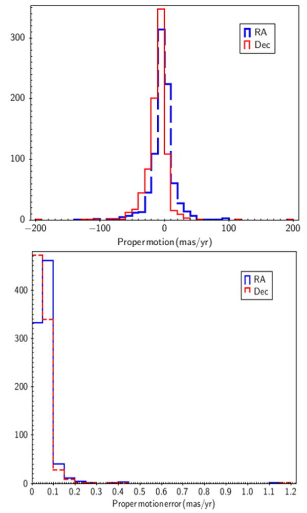
Figure 4: Distribution of proper motions and their error for our sample in both right ascension and declination.

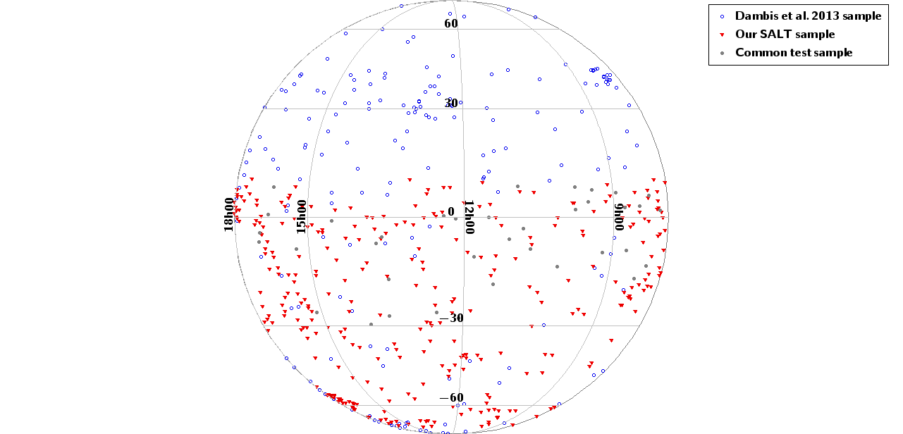
Figure 5: Sky distribution of the total 850 RRL samples. Our new addition samples from our SALT observation and Dambis et al., 2013 compilation are shown with filled read triangles and open blue circles, respectively. 40 RRLs with both spectroscopic data which uses as the test sample for our observation are shown with filled gray circles.

2.4 Abundances

Abundances data for our sample RRLs were not available in public release surveys like SDSS, Gaia and others when we started this study. Thus, like the case of other data types, we adopted homogenized metallicities on the Zinn & West (1984) scale from two primary sources: our previous compilation (Dambis et al., 2013) for the first part of our sample stars, and our new SALT spectroscopic observations for the remaining part. However, the metallicity for CK Uma was not included in Dambis et al. (2013) compilation. Therefore, we adopted the metallicity for this star from LAMOST survey (Luo et al., 2012).

Our SALT spectroscopic observations were performed using the Robert Stobie Spectrograph (RSS; Burgh et al., 2003; Kobulnicky et al., 2003) in the long-slit mode. The VPH grating GR1300 and 1.25 arcsec slit width were used for observations during 2016 and 2017. This configuration produces spectral resolution R = 1300-1500 and covers spectral range of 3900–6000 Å, which gives us a possibility to detect Balmer lines H$\alpha$, H$\beta$, H$\gamma$ and CaII K $\lambda$3924 line. These SALT spectroscopic observations were primary reduced using the SALT science pipeline (Crawford et al., 2010) as the long-slit reduction were done automatically in the way described in Kniazev et al. (2008) with our pipeline based on MIDAS, Unix Shell and IRAF programs. Here, we also used ULySS program by Koleva et al. (2009) with a medium spectral-resolution library of Prugniel et al. (2011) to determine simultaneously the line-of-sight velocities, T_eff, log g and [Fe/H] for the observed stars. Details of these reduction routines and their accuracy with our RSS data for a particular MAGIG project star was presented in Kniazev et al. (2019) and more detail for RRL samples of the project will also be presented in a forthcoming paper (Kniazev et al. 2020, in preparation).

In order to make the measurement scale of our SALT abundances homogeneous with our previous compilation scale, we calibrated our pipeline abundance measurements to our previous published Zinn & West (1984) scale using subsample of RRLs, which have abundance measurement in both scales. Based on this calibration, we find SALT metallicity scale transformation equation (2) to Zinn & West (1984) metalliciity scale:

$$[Fe/H]_{ZW}=(0.836~{}\pm~{}0.053)[Fe/H]_{SALT}-(0.323~{}\pm~{}0.082)$$ (2)

with a scatter of 0.23dex. Our abundances are measured at random phase and we apply no phase corrections. The point is that although generally the inferred spectroscopic abundances of RR Lyraes vary with phase (Pancino et al., 2015), in our particular case the abundances inferred using ULySS program by Koleva et al. (2009) combined with the medium of Prugniel et al. (2011) appear to be phase independent (see Fig. 6, where the difference between our SALT RR Lyrae abundances and previous measurements is plotted against the phase of our SALT observations).

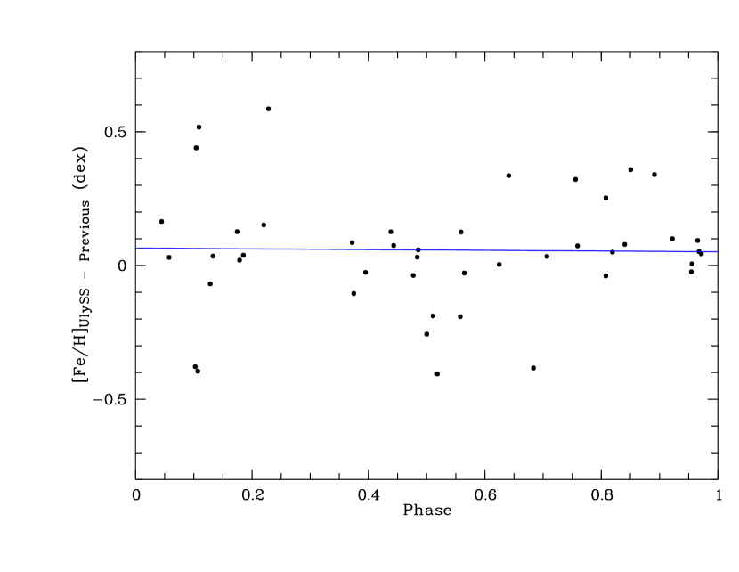
Figure 6: The difference between our abundance estimates based on SALT spectra and the previously published values for the calibrating subsample. Note the absence of any appreciable phase trend.

Whenever necessary, we also made transformation to the modern scale of Carretta et al. (2009) via equation

$$[Fe/H]_{Carr}=1.105[Fe/H]_{ZW}+0.160$$ (3)

with a slightly increased scatter of 0.25dex. The formal internal errors of the inferred metallicities are too small (generally on the order of 0.01–0.05) to be realistic, and we therefore estimate errors based on a comparison with published data (see equation 2 above). We assume that the average errors of the adopted metallicities are the same for all stars whether based on SALT spectra or on published data as presented in our earlier list (Dambis et al., 2013). Given the scatter of equation 2 (0.23dex), the adopted metallicities are accurate to within 0.23dex/$\sqrt{2}$ = 0.16dex.

Fig. 7 compares our measured metallicities transformed to the Carretta et al. (2009) scale (equations 2 and 3 above) with their available Gaia DR2 metallicity (Gaia Collaboration et al., 2019), which were estimated from the Fourier coefficients of Gaia photometric data. Thus, our metallicity measurements and Gaia DR2 data generally agree for stars which have reliable Gaia photometry, but our measurements are more prices.

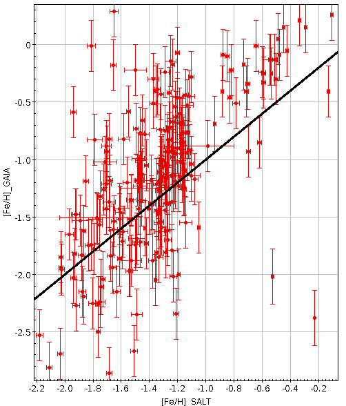
Figure 7: Comparison between our SALT [Fe/H] with their available Gaia DR2 data. The solid line represent the bisector

Finally, these homogeneous metallicities on the Zinn & West (1984) scale with their corresponding errors and source of references for our total 850 sample RRLs are available in column 7 and 8 of Table 2, respectively. As can be seen in Fig. 8, the metallicity distribution of the total sample span quite a broad range; namely, from $-$2.84 to +0.07 dex, and its peak lies between -1.2 and -1.5 dex.

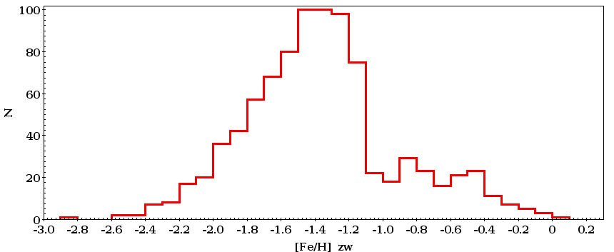
Figure 8: Distribution of [Fe/H] values for RRL variables of our total sample transformed to the Zinn and West scale.

2.5 Radial velocities

Like for metallicity, we adopt the mean radial velocities $(V_{R})$ and standard errors $(\sigma_{V_{R}})$ for the first and second parts of our RRL sample from our previous publication (Dambis et al., 2013) and from our SALT spectroscopic, respectively. We used our SALT H$\alpha$, H$\beta$, H$\gamma$ (Balmer) and CaIIK spectral line observations first to estimate the measured radial velocity at specific phases of pulsation. Then, the precise systematic (center of mass) velocities in the radial direction of RRLs are determined by subtracting the radial velocity due to pulsation at same phase from our highly precise measured radial velocities.

Given that the combination of spectral lines and the procedure we use to measure the radial velocities differ from those employed by other authors, we cannot apply the published formulas and scaling procedures verbatim. The proper way would be to derive our own template radial-velocity curve and scaling relations by observing some stars at several phases with good enough sampling. Unfortunately, this approach was inapplicable in our case because most of the stars with SALT data (461 out of 488) were observed only once, 25 stars were observed twice, and one star was observed three times. We therefore decided to use a published template by properly scaling and shifting it in phase (applying a phase lag). Fig. 9 shows the velocity corrections for the test sample (44 measurements for 40 stars from the list of Dambis et al. (2013) with SALT observation) plotted against phase. A clear phase dependence is immediately apparent, which we fitted by the Liu (1991) template $-S(\phi)-$ by finding the scaling factor and appropriate offsets in both phase and velocity difference. The least-squares fit yields the following result:

$$V_{R}{sys}-V_{R}(SALT)=-(38.6~{}\pm~{}5.8)+$$ (4)

$$(62.0~{}\pm~{}9.3)S(\phi-0.130~{}\pm~{}0.015)$$

with a scatter of 20.5 km/s.

One would naturally expect the errors of $V_{R}{sys}$ inferred from $V_{R}(SALT)$ via equation 4 to depend on the quality of spectra (quantified by the signal-to-noise ratio). We binned our test list of SALT radial-velocity measurements for RR Lyraes with published systemic velocities into five bins by signal-to-noise ratio and found the scatter of the difference between the published systemic velocities and those inferred from SALT data (after quadratically subtracting the errors of published velocities) to be inversely proportional to the signal-to-noise error, $\sigma_{V}(SALT)~{}\sim~{}1223/SNR$ (see Fig. 10). We use this relation to estimate the errors of all individual radial-velocity measurements based on SALT data. These measurements have SNR values spanning from 11.4 to 154.4, implying a range of radial-velocity errors from 8 to 107 km/s. Because of the repeated measurements for a number of stars the errors of the mean radial-velocity estimates actually span from 5.6 to 107 km/s with an average value of 18.8 km/s.

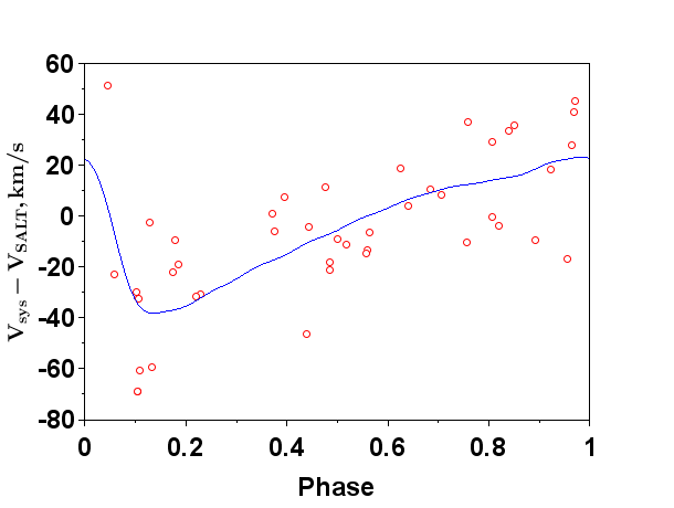
Figure 9: Dependence of the velocity correction, $V_{sys}$ - $V_{SALT}$, on the phase of spectroscopic observations for the test sample stars. The fit of the Liu (1991) template scaled and shifted in both coordinates (see equation 4) is shown by the continuous line.

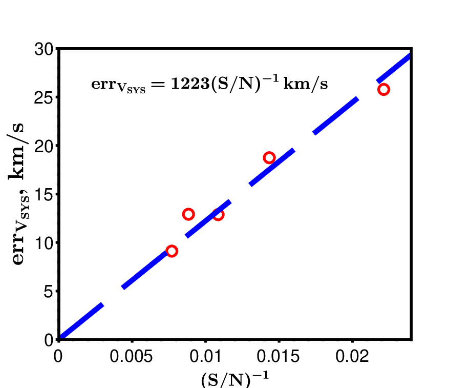
Figure 10: Dependence of the scatter of the previously published systemic velocity, $V_{sys}$, and our phase-corrected radial velocity, $V_{SALT}$, on signal-to-noise ratio.

Fig. 11 compares our measured radial velocities with available Gaia DR2 data (Sartoretti et al., 2018). Thus our radial velocity measurements are in excellent agreement with available Gaia DR2 data.

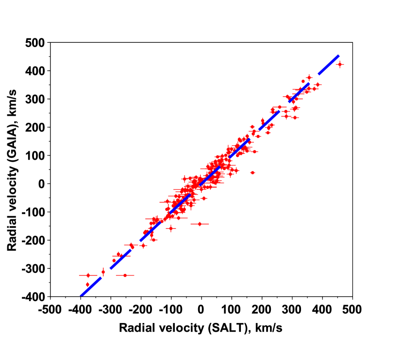
Figure 11: Comparison between our measured radial velocity with their available Gaia DR2 data.

The systemic (center of mass) radial velocities $(V_{R})$ with standard errors and the corresponding references for our total sample RRLs are presented in columns 15 and 16 of Table 2, respectively. Fig. 12 shows the distribution of radial velocity errors for all of our sample stars. As noted from Fig. 12, the precision of radial velocities for most of our sample RRLs are better than 16km/s thereby contributing to accurate modeling of the kinematics of RRLs.

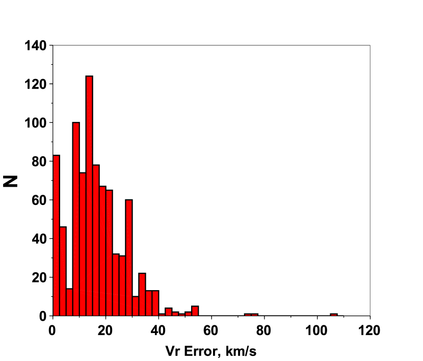
Figure 12: Distribution of radial velocity errors for sample stars.

2.6 Interstellar Extinction and Intrinsic colour calibrations

Similarly to our previous work (Dambis et al., 2013), we begin by estimating interstellar extinction toward our RRLs via the Drimmel et al. (2003) 3D extinction model using the iterative procedure described in detail in that paper. The procedure consists of (1) setting the starting extinction values $A_{V}$ = $A_{W1}$ = $A_{KS}$ to zero; (2) computing the provisional photometric distances to the stars based on their apparent infrared magnitudes, the corresponding absolute magnitudes determined via the appropriate period-metallicity-luminosity relation, and the currently adopted provisional extinction values; (3) updating the $A_{V}$ extinction values by estimating them via the 3D map of Drimmel et al. (2003) based on the sky positions and provisional distances inferred at stage (2) and computing the $A_{W1}$ and $A_{Ks}$ extinction values by converting the inferred $A_{V}$ using the Yuan et al. (2013) extinction coefficients $R_{V}=3.1$, $R_{W1}=0.18$, and $R_{Ks}$=0.306, and (4) repeating steps (2)–(3) with the updated extinction values until the latter converge. We adopt the Dambis et al. (2014) WISE W1-band PLZ relation in Zinn & West (1984) metallicity scale:

$$\begin{array}[]{rcl}\langle M_{W1}\rangle&=&-0.814+0.106[Fe/H]-2.381\log P_{F},\end{array}$$ (5)

to compute the initial distances for the subsample of RRLs (846 stars) that have either measured intensity-mean magnitude or single exposure data in $W1$-band. For the four RRLs without the $W1$-band magnitude data, we used the corresponding period-metallicity-$M_{K}s$ relation

$$\begin{array}[]{rcl}\langle M_{Ks}\rangle&=&-0.769+0.088[Fe/H]-2.33\log P_{F},\end{array}$$ (6)

derived by Dambis et al. (2013).

In principle, we could use the $A_{V}$, $A_{Ks}$, and $A_{W1}$ extinction estimates so derived to calibrate the intrinsic colors $(V-Ks)_{0}$ and $(V-W1)_{0}$ in terms of fundamentalized period and metallicity. The procedure is as follows. First, deredden the intensity-mean magnitudes of our RR Lyraes in the W1-band $-\langle m_{W1}\rangle$, Ks-band $-\langle m_{Ks}\rangle-$ and $V$-band $-\langle m_{V}\rangle-$ by their corresponding interstellar extinction values ($A_{W1}$, $A_{Ks}$ and $A_{V}$, respectively):

$$\langle W1\rangle_{0} = \langle m_{W1}\rangle-A_{W1}$$ (7)

$$\langle Ks\rangle_{0} = \langle m_{Ks}\rangle-A_{Ks}$$ (8)

$$\langle V\rangle_{0} = \langle m_{V}\rangle-A_{V}$$ (9)

We then use equations (7), (8) and (9) to compute the intrinsic colours:

$$\begin{array}[]{rcl}(V-Ks)_{0}&=&\langle V\rangle_{0}-\langle Ks\rangle_{0}\\ &=&\langle m_{V}\rangle-\langle m_{Ks}\rangle-(A_{V}-A_{Ks})\end{array}$$ (10)

$$\begin{array}[]{rcl}(V-W1)_{0}&=&\langle V\rangle_{0}-\langle W1\rangle_{0}\\ &=&\langle m_{V}\rangle-\langle m_{W1}\rangle-(A_{V}-A_{W1})\end{array}$$ (11)

We now calibrate the $(V-W1)_{0}$ and $(V-Ks)_{0}$ colours using the following two well-established assumptions: first, that $M_{V}$ depends linearly on $[Fe/H]$ and does not depend on period at constant $[Fe/H]$ (see, e.g., Catelan et al., 2004):

$$\langle M_{V}\rangle=a_{V}+b_{V}[Fe/H].$$ (12)

and, second, that $<M_{W1}>$ and $<M_{Ks}>$ depend linearly on $[Fe/H]$ and log $P_{F}$:

$$\langle M_{Ks}\rangle=a_{K}+b_{K}[Fe/H]+c_{K}\log P_{F}$$ (13)

and

$$\langle M_{W1}\rangle=a_{W}+b_{W}[Fe/H]+c_{W}\log P_{F}$$ (14)

We further adopt the metallicity slope $b_{V}$ = 0.232 for the $V$-band metallicity-luminosity relation, so that:

$$\langle M_{V}\rangle=a_{V}+0.232[Fe/H].$$ (15)

This slope is based on the two direct estimates (Gratton et al., 2004), which involve RR Lyrae in the LMC (believed to be at approximately the same distance) and the the horizontal branches in M31 satellite galaxies (Federici et al., 2012) (also believed to be at approximately the same distance from us), respectively. As we pointed out earlier (Dambis et al., 2013), the adopted metallicity slope is also quite consistent with the estimates based on Baade-Wesselink analysis (Cacciari et al., 1992). We finally adopt the period slopes of the 2MASS $Ks$- and WISE $W1$-band period-metallicity-luminosity relations from Jones et al. (1992) and Dambis et al. (2014), respectively, where they are estimated from the data for RR Lyraes in globular clusters, so that equations 13 and 14 become:

$$\langle M_{Ks}\rangle=a_{K}+b_{K}[Fe/H]-2.33\log P_{F}$$ (16)

and

$$\langle M_{W1}\rangle=a_{W}+b_{W}[Fe/H]-2.381\log P_{F},$$ (17)

respectively. We now subtract equations (16) and (17) from equation (15) to obtain:

$$\begin{array}[]{rcl}(V-Ks)_{0}&=&\langle M_{V}\rangle-\langle M_{Ks}\rangle\\ &=&(a_{V}-a_{K})+(0.232-b_{K})[Fe/\\ &&H]+2.33\log P_{F}.\end{array}$$ (18)

and

$$\begin{array}[]{rcl}(V-W1)_{0}&=&\langle M_{V}\rangle-\langle M_{W1}\rangle\\ &=&(a_{V}-a_{W})+(0.232-b_{W})[Fe/\\ &&H]+2.381\log P_{F}.\end{array}$$ (19)

We then move the period terms to the left-hand side:

$$(V-Ks)_{0}-2.33\log P_{F}=(a_{V}-a_{K})+(0.232-b_{K})[Fe/H].$$ (20)

and

$$(V-W1)_{0}-2.381\log P_{F}=(a_{V}-a_{W})+(0.232-b_{W})[Fe/H].$$ (21)

We can now solve sets of linear equations (20) and (21) with the unknowns being $a_{V}-a_{K}$, (0.232-$b_{K}$) and $a_{V}-a_{W}$,(0.232-$b_{W}$) for our RR Lyraes to obtain the desired calibrations of the intrinsic colours $(V-Ks)_{0}$ and $(V-W1)_{0}$ in terms of fundamentalized period and metallicity. The resulting 3$\sigma$-clipped least-squares solutions are

$$\begin{array}[]{rcl}(V-Ks)_{0}&=&1.751(\pm 0.020)+0.115(\pm 0.013)[\\ &&Fe/H]+2.33\log P_{F}\\ \end{array}$$ (22)

with a scatter of $\sigma(V-Ks)_{0}=0.175$ (791 of 850 stars) and

$$\begin{array}[]{rcl}(V-W1)_{0}&=&1.903(\pm 0.016)+0.155(\pm 0.011)[\\ &&Fe/H]+2.381\log P_{F}\\ \end{array}$$ (23)

with a scatter of $\sigma(V-W1)_{0}=0.137$ (768 of 846 stars).

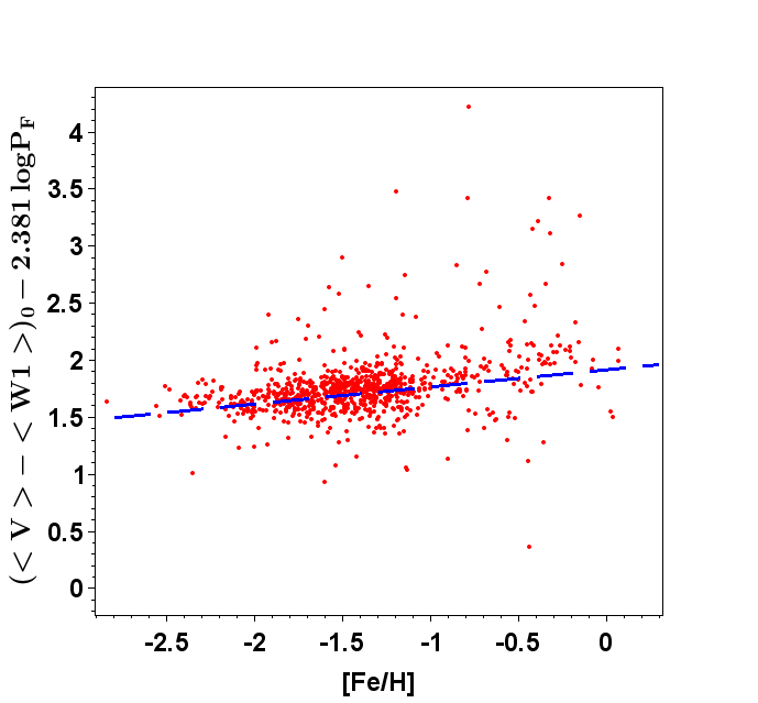
Figure 13: Plot of $(V-W1)_{0}-2.381\log P_{F}$ as a function of $[Fe/H]$. The solid line shows the linear fit (equation (21)) with parameters (23)

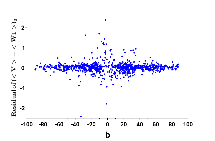
Figure 14: Plot of residual of $(V-W1)_{0}$ (equation (21)) as a function of $b$.

Fig. 13 shows the plot of equation (21) for all 846 RRLs with linear fitting with parameters from (23) superimposed, and Fig. 14 shows the plot of its residuals as a function of Galactic latitude. The most interesting feature of Fig. 14 is that residuals decrease sharply for $|b|\geq 40^{0}$, which indicates that the Drimmel et al. (2003) 3D extinction model is accurate for high Galactic latitudes as suggested in Dambis et al. (2013). We therefore perform new fits based on 271 and 308 RR Lyraes located at $|b|>40^{0}$ (recall that in the case of the $(V-Ks)_{0}$ calibration we use only phase-corrected $K_{s}$-band data for the total subsample):

$$\begin{array}[]{rcl}(V-Ks)_{0}&=&1.834(\pm 0.028)+0.131(\pm 0.018)[\\ &&Fe/H]+2.33\log P_{F}\\ \end{array}$$ (24)

with a scatter of $\sigma(V-Ks)_{0}=0.113$ (264 of 271 stars) and

$$\begin{array}[]{rcl}(V-W1)_{0}&=&1.865(\pm 0.022)+0.108(\pm 0.014)[\\ &&Fe/H]+2.381\log P_{F}\\ \end{array}$$ (25)

with a scatter of $\sigma(V-W1)_{0}=0.094$ (299 of 308 stars) and finally adopt these period-luminosity-colour relations for RR Lyraes.

Hence 0.232 - $b_{K}$ = 0.108 and 0.232 - $b_{W}$ = 0.108, implying that $b_{K}$ = 0.101 and $b_{W}$ = 0.124. Given equations (16) and (17) it follows from this that

$$\langle M_{Ks}\rangle=a_{K}+0.101[Fe/H]-2.33\log P_{F}$$ (26)

and

$$\langle M_{W1}\rangle=a_{W}+0.124[Fe/H]-2.381\log P_{F},$$ (27)

respectively. To make the adopted PLZ relations maximally consistent with those inferred by Dambis et al. (2013) and Dambis et al. (2014), respectively, we set the zero points $a_{K}$ and $a_{W}$ so as to obtain the same absolute magnitudes at the average metallicity and average logarithm of the fundamenalised period for our RR Lyrae sample ($<[Fe/H]>$ =-1.39 and $<\log P_{F}>$ = -0.277), so that:

$$\langle M_{Ks}\rangle=-0.809+0.101[Fe/H]-2.33\log P_{F}$$ (28)

and

$$\langle M_{W1}\rangle=-0.789+0.124[Fe/H]-2.381\log P_{F},$$ (29)

respectively and it is these relations that we use below to compute our initial RR Lyrae distances for the statistical-parallax analysis. Note that the dependence of the $A_{V}$ reddening estimates for RR Lyraes at high Galactic latitudes, which are based on the 3D interstellar extinction model by Drimmel et al. (2003) on the adopted PLZ relation, is negligible as we found earlier by comparing the extinction values computed with RR Lyrae distances inferred using different PLZ relations: the mean offset is of about +0.0002 $\pm$0.0001 with a scatter of 0.0016 (Dambis et al., 2013).

It is not safe to use extinction values derived from the 3D map at low Galactic latitudes, where the clumpy distribution of absorbing matter makes such estimates rather inaccurate and too sensitive to distance errors. We therefore finally determined the interstellar extinction for 541 RRLs that are located at low galactic latitudes ($|b|\leq 40^{0}$) from their $E(V-W1)$ (538 stars) or $E(V-Ks)$ (3 stars) colour excess based on period-metallicity-colour relations (24) and (25) above by converting the latter into $E(B-V)$ and interstellar extinction values ($A_{V},A_{Ks},A_{W1}$) adopting the Yuan et al. (2013) extinction coefficients.

In Fig. 15, we compared our V-band interstellar extinction determined by using our calibrated colour relations for our sample RRLs with their available Gaia DR2 values(Gaia Collaboration et al., 2019). In this case, the values of $A_{G}$ in Gaia G-band photometry were converted to $A_{V}$ using the extinction coefficient of Chen et al. (2018b) ($R_{G}=2.5$) to be consistent with Yuan et al. (2013) extinction coefficients. The lower left corner of Fig. 15 shows the nice agreement existing between our interstellar extinction and Gaia estimation for lower values; on the contrary, there is less agreement for larger extinction values which may be due to less information obtained from the three broad Gaia pass bands to estimate larger extinction values (Anders et al., 2019). Hence, caution must be taken to use Gaia DR2 extinction values as suggested by Arenou et al. (2018). The final V-band interstellar extinction values ($A_{V}$) for our total sample RRLs are presented in column 9 of Table 2.

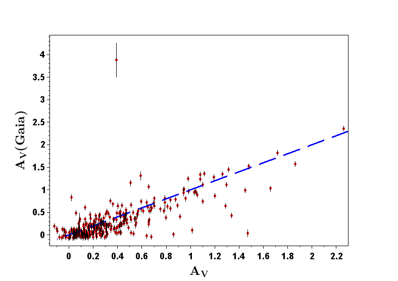
Figure 15: Comparison between the V-band interstellar extinction derived via our calibrated colour relations and Gaia DR2.The broken line represents the bisector.

2.7 Final Database

Using the data sources described above, we constructed a database for a total of 850 RRLs as presented in Table 2 (the full version will be available in the CDS and in the online version of the article–see Supporting Information). The columns of this table are the following: (1) the GCVS name of the star; (2) and (3) its J2000.0 equatorial coordinates $\alpha$ and $\delta$, respectively, in decimal degrees; (4) the variability period in days; (5) the RRL type (AB or C); (6) and (7) the V-band intensity-mean magnitude $<m_{V}>$ with its error and data source reference code (Ref: 1 for our observation; 2 for Gaia DR2 and 3 for Dambis et al. (2013) catalog), respectively; (8) the V-band interstellar extinction $A_{V}$; (9) and (10) the metallicity [Fe/H] on the Zinn & West (1984) scale with its error and data source reference code (Ref: 1 for our observation and 3 for Dambis et al. (2013) catalog); (11) and (12) the Ks-band intensity-mean magnitude $<Ks>$ or 2MASS single epoch magnitude with its error $\sigma_{Ks}$ and data source reference code (Ref: 7 for 2MASS single epoch observation, 8 for Layden et al. (2019) and 9 for mean estimation in this paper and Dambis et al. (2013)), respectively; (13) and (14) the W1-band intensity-mean magnitude $<W1>$ or WISE single epoch magnitude with its errors $\sigma_{W1}$ and data source reference code (Ref: 3 for Dambis et al. (2013) catalog, 4 for Chen et al. (2018a) catalog, 5 for Gavrilchenko et al. (2014) catalog and 6 for ALL WISE single epoch magnitudes), respectively; (15) and (16) the average radial velocity $V_{R}$ with its standard error $\sigma V_{R}$ (both in  km s^-1) and data source reference code (Ref: 1 for our observation and 3 for Dambis et al. (2013) catalog), respectively; (17)-(19) the Gaia DR2 proper motion in  mas yr^-1 to the right ascension ($\mu_{\alpha}$) and declination $(\mu_{\delta})$ and parallax in mas with their corresponding standard errors, respectively.

Table 2: The first 10 lines of the total 850 Galactic field RRL variables database. This is a sample of the full version, which is available in the CDS and the online version of the article (see Supporting Information).

(1)	(2)	(3)	(4)	(5)	(6)	(7)	(8)	(9)	(10)	(11)	(12)	(13)	(14)
Name	$\alpha$	$\delta$	Period	Type	$<V>$	Ref	Av	[Fe/H]	Ref	$<Ks>$	Ref	$<W1>$	Ref
SW And	5.92954	29.401022	0.4423	RRAB	9.712 $\pm$0.009	3	0.28408	-0.38$\pm$ -	3	8.511 $\pm$0.009	8	8.464 $\pm$0.009	3
XX And	19.3642	38.950554	0.7228	RRAB	10.687$\pm$0.009	3	-0.00359	-2.01$\pm$ -	3	9.442 $\pm$0.027	8	9.378 $\pm$0.006	3
ZZ And	12.3952	27.02213	0.5545	RRAB	13.082$\pm$0.018	3	0.21469	-1.58$\pm$ -	3	11.834$\pm$0.035	9	11.795$\pm$0.01	3
XY And	21.6768	34.06858	0.3987	RRAB	13.68 $\pm$0.019	3	0.26325	-0.92$\pm$ -	3	12.892$\pm$0.04	9	12.617$\pm$0.005	3
BK And	353.775	41.102886	0.4216	RRAB	12.97 $\pm$0.037	3	0.397	-0.08$\pm$ -	3	11.663$\pm$0.04	9	11.614$\pm$0.008	3
BK Ant	146.062	-39.6613	0.5166	RRAB	11.799$\pm$ -	2	0.13406	-0.519$\pm$0.16	1	10.614 $\pm$0.04	9	10.547$\pm$0.023	4
BN Ant	149.275	-39.2906	0.5359	RRAB	12.488$\pm$ -	2	0.31463	-1.25$\pm$0.16	1	11.146$\pm$0.04	9	11.107$\pm$0.023	4
RT Ant	143.064	-25.1997	0.553	RRAB	14.198$\pm$ -	1	0.29522	-1.48$\pm$0.16	1	12.878$\pm$0.038	7	12.828$\pm$0.024	6
SS Ant	144.795	-26.5519	0.4837	RRAB	13.526$\pm$ -	2	0.28575	-1.42$\pm$0.16	1	12.582$\pm$0.04	9	12.463$\pm$0.024	5
UZ Ant	166.334	-38.9462	0.6003	RRAB	14.0 $\pm$ -	2	0.24006	-1.75$\pm$0.16	1	12.361$\pm$0.042	7	12.354$\pm$0.023	5
(1)	(15)	(16)	(17)	(18)	(19)
Name	$V_{R}$	Ref	$\mu_{\alpha}\pm\sigma\mu_{\alpha}$	$\mu_{\delta}\pm\sigma\mu_{\delta}$	$\varpi\pm\sigma\varpi$
SW And	-21.0$\pm$1.0	3	-6.8 $\pm$0.1	-19.3$\pm$0.3	1.7797$\pm$0.1636
XX And	0.0 $\pm$1.0	3	58.1 $\pm$0.1	-32.9$\pm$0.1	0.695 $\pm$0.0463
ZZ And	-13.0$\pm$53.0	3	31.6 $\pm$0.1	-17.5$\pm$0.0	0.3148$\pm$0.0273
XY And	-64.0$\pm$53.0	3	11.3 $\pm$0.1	-9.0 $\pm$0.1	0.338 $\pm$0.0429
BK And	-17.0$\pm$7.0	3	6.3 $\pm$0.0	-1.4 $\pm$0.0	0.445 $\pm$0.0281
BK Ant	30.4$\pm$10.5	1	0.3 $\pm$0.0	-3.3 $\pm$0.0	0.6422$\pm$0.0304
BN Ant	258.4$\pm$22.8	1	24.1 $\pm$0.0	-26.8$\pm$0.0	0.4264$\pm$0.0278
RT Ant	396.0$\pm$24.0	1	-4.8 $\pm$0.1	-2.3 $\pm$0.1	0.2202$\pm$0.0327
SS Ant	45.7 $\pm$18.3	1	9.8 $\pm$0.1	-15.4$\pm$0.1	0.1652$\pm$0.033
UZ Ant	515.7$\pm$11.2	1	-17.6$\pm$0.0	-5.8 $\pm$0.0	0.1884$\pm$0.0244

3 Method

As we pointed out earlier, this research uses the bimodal version of maximum-likelihood statistical parallax method to calibrate the zero points of LZ and PLZ relations of RRLs in visual and IR bands, and to estimate the kinematical parameters of RRLs population in the disk and halo of our Galaxy. Here, we present the basic ideas and notation of the method as described in section 2.4 of Dambis (2009); for detailed step-by-step instructions see the papers by Hawley et al. (1986) and Dambis (2009).

We begin by computing the assumed distances in kpc for our sample RRLs using

$$D_{A}=10^{0.2(\langle m_{x}\rangle-A_{x}-M_{A,x})-2}$$ (30)

where $\langle m_{x}\rangle$, $M_{A,x}$ and $A_{x}$ are the apparent mean magnitude, the adopted absolute magnitude and interstellar extinction in x band, respectively. For reasons that are mentioned in section 1 and additional explanations in the next section 4, we estimated $M_{A}$ for almost all of our sample RRLs by adopting the above calibrated W1-band PLZ relation of Dambis et al. (2014) (eq. 29). However, for four RRLs that have no measured $\langle m_{W1}\rangle$, we adopted Ks- band PLZ relation (eq. 28) which is consistent with the above W1-band PLZ relation. Thus, our aim is to use the statistical-parallax technique to determine the absolute-magnitude correction for the adopted PLZ relations ($\Delta M;M_{true}=M_{A}+\Delta M$), which is related to the inverse distance-scale correction factor ($f=D_{A}/D$; the assumed distance divided by the real or true distance) in such a way that $f=10^{0.2\times\Delta M}$.

Using the assumed distance-$D_{A}$ a residual velocity ($\mn@boldsymbol{\nu}$) for a given local homogeneous sample, which is equal to the observed velocity minus the velocity implied by the adopted model, can be calculated:

$$\mn@boldsymbol{\nu}=|\mn@boldsymbol{D_{A}}|\mn@boldsymbol{\mu_{obs}}+V_{R(obs)}\hat{\mn@boldsymbol{r}}-[f\mn@boldsymbol{\Pi}+\mn@boldsymbol{\hat{r}\hat{r}}^{\prime}](\mn@boldsymbol{\bar{V}-\bar{V}_{\odot}}),$$ (31)

where $\mn@boldsymbol{\mu_{obs}}$, $\mn@boldsymbol{V_{R(obs)}}$ $\mn@boldsymbol{\bar{V}}$ and $\mn@boldsymbol{\bar{V}_{\odot}}$ are observed proper motion, radial velocity, relative bulk (average) velocity of the sample star and the Sun with respect to the adopted reference frame, respectively; $\mn@boldsymbol{\hat{r}}$- is the unit vector pointing radially towards the star and $\mn@boldsymbol{\hat{r}}^{\prime}$- is its transpose; $\mn@boldsymbol{\hat{r}\hat{r}}^{\prime}$ is the matrix of projection on to the line of sight; $\mn@boldsymbol{\Pi=U-\hat{r}\hat{r}}^{\prime}$ is the matrix of projection on to the sky plane, and U is the unit matrix. Here, $\mn@boldsymbol{\bar{V}-\bar{V}_{\odot}}$ is one of the unknown model parameters that we need to determine.

Thus, the matrix of covariance (M), which is the covariances tensor of $\mn@boldsymbol{\nu}$, can be computed in terms of the assumed distance of the star, the distance-scale correction factor f, the random error of the distance-scale parameter ($\delta f$), the observational errors of proper motions ($\delta\mu$) and the standard error of the radial velocity $(\delta V_{R})$:

$$\begin{array}[]{rcl}\textbf{M}&=&\displaystyle cov(\mn@boldsymbol{\nu})=\langle\delta\mn@boldsymbol{\nu}\delta\mn@boldsymbol{\nu}^{\prime}\rangle=|\mn@boldsymbol{D_{A}}|^{2}\langle\delta\mn@boldsymbol{\mu}\delta\mn@boldsymbol{\mu}^{\prime}\rangle+\\ &&\displaystyle(\hat{\mn@boldsymbol{r}}\hat{\mn@boldsymbol{r}}^{\prime})\delta V_{R}^{2}+[f\mn@boldsymbol{\Pi}+\mn@boldsymbol{\hat{r}\hat{r}}^{\prime}]\mn@boldsymbol{\Sigma}[f\mn@boldsymbol{\Pi}+\mn@boldsymbol{\hat{r}\hat{r}}^{\prime}]^{\prime}+\\ &&\displaystyle\delta f^{2}\mn@boldsymbol{\Pi}[(\mn@boldsymbol{\bar{V}-\bar{V}_{\odot})(\bar{V}-\bar{V}_{\odot})}^{\prime}+\mn@boldsymbol{\Sigma}]\mn@boldsymbol{\Pi}^{\prime}\end{array},$$ (32)

where $\mn@boldsymbol{\Sigma}$ is the covariance tensor of true residual velocities at the location of the star (the velocity ellipsoid), and this is also another unknown model parameter that we are supposed to determine.

If we assume that residual velocities $\mn@boldsymbol{\nu}$ obey a three-dimensional Gaussian distribution with zero mean and a covariance tensor M in the local homogeneous sample, then the likelihood of obtaining all observations simultaneously for N-stars can be expressed as

$$\begin{array}[]{rcl}L&=&\displaystyle\prod_{i=1}^{N}prob(\mn@boldsymbol{\nu}_{i})\\ &=&\displaystyle\prod_{i=1}^{N}\{(2\pi)^{-\frac{3}{2}}|\textbf{M}|_{i}^{-\frac{1}{2}}\exp(-0.5\mn@boldsymbol{\nu}^{\prime}_{i}\textbf{M}_{i}^{-1}\mn@boldsymbol{\nu}_{i})\},\end{array}$$ (33)

where $|\textbf{M}|_{i}$ and $\mn@boldsymbol{\nu}^{\prime}_{i}$ denotes the determinant of the covariance tensor and the transpose of residual velocity vector for specific star i, respectively. Hence, the distribution function has the meaning of the probability density for the residual velocity of a particular star, and given that stars are distributed independently of each other in the velocity space, their N- point distribution function is equal to the product of functions for all stars of the sample. Therefore, the logarithm of the likelihood of obtaining all observations simultaneously becomes

$$\begin{array}[]{rcl}\ln L&=&\displaystyle\sum_{i=1}^{N}\ln prob(\mn@boldsymbol{\nu}_{i})\\ &=&\displaystyle-0.5\sum_{i=1}^{N}(\ln|\textbf{M}|_{i}+\mn@boldsymbol{\nu}_{i}^{{}^{\prime}}\textbf{M}^{-1}_{i}\mn@boldsymbol{\nu_{i}})+\frac{3}{2}(2\pi)N\end{array}$$ (34)

However, our sample is not homogeneous as it contains two purportedly homogeneous subsamples (Disk and Halo), each of which obeys its own three-dimensional residual velocity distribution and each object may priorly belong to any of the two subsamples. In this case, the residual velocity distributions for any specific star i becomes

$$\begin{array}[]{rcl}prob(\mn@boldsymbol{\nu}_{i})&=&\displaystyle\alpha\times(2\pi)^{-\frac{3}{2}}|\textbf{M}_{1}|^{-\frac{1}{2}}\exp(-0.5\mn@boldsymbol{\nu}^{\prime}_{1}\textbf{M}_{1}^{-1}\\ &&\mn@boldsymbol{\nu}_{1})+(1-\alpha)\times(2\pi)^{-\frac{3}{2}}|\textbf{M}_{2}|^{-\frac{1}{2}}\\ &&\exp(-0.5\mn@boldsymbol{\nu}^{\prime}_{2}\textbf{M}^{-1}_{2}\mn@boldsymbol{\nu}_{2}),\end{array}$$ (35)

where $\alpha$ and $1-\alpha$ are the number fractions of the halo (j=1) and disk (j=2) subsamples (prior probability for a single star i to be in halo and disk subsamples) and these are unknown parameters that we need to estimate; $\mn@boldsymbol{\nu}_{j}$ are the residual velocities of the specified star i with respect to $j^{th}$ subsample, which can also be expressed as

$$\mn@boldsymbol{\nu}_{j}=|\mn@boldsymbol{D_{A}}|\mn@boldsymbol{\mu}_{obs}+V_{R(obs)}\,\,\mn@boldsymbol{\hat{r}}-[f\mn@boldsymbol{\Pi}+\mn@boldsymbol{\hat{r}\hat{r}}^{\prime}](\mn@boldsymbol{\bar{V}}_{j}-\mn@boldsymbol{\bar{V}}_{\odot j});$$ (36)

here, $\mn@boldsymbol{\bar{V}}_{j}$ and $\mn@boldsymbol{\bar{V}}_{\odot j}$ are the average velocity of the $j^{th}$ subsample stars and the Sun at the specified star i location with respect to the adopted reference frame, respectively, and $\textbf{M}_{j},j=1,2$ are the corresponding covariance tensors.

When we express the likelihood function ($\ln L$) of the bimodal RRL population distribution function (equation 35) in terms of the observable quantities and the model parameters to be determined, the likelihood function depends on 14 unknown model parameters: the three components of the relative bulk motion of the halo, ($U_{0}$, $V_{0}$, $W_{0}$)_Halo and disk, ($U_{0}$, $V_{0}$, $W_{0}$)_Disk, RRL subsamples with respect to the Sun (the reflex solar motion with respect to the sample stars); the three diagonal components of the velocity ellipsoid of the halo, $(\sigma V_{R}$, $\sigma V_{\phi}$, $\sigma V_{\theta})_{Halo}$ and disk, $(\sigma V_{R}$, $\sigma V_{\phi}$, $\sigma V_{\theta})_{Disk}$, RRL components; the inverse distance-scale correction factor (f), and the fraction of RRLs that belong to halo component ($\alpha$). To this end, we adopt the peculiar velocity of sun to be (+9, +12, +7) km/s (Mihalas & Binney, 1981) and the local standard of rest velocity to be 220 km/s (Kerr & Lynden-Bell, 1986) in the Cartesian Galactic system.

Thus, the best values of these 14 model parameters were determined according to the principle of maximum likelihood by maximizing $\ln L$, which is equivalent to minimizing $-\ln L$, using the numerical method of minimization without evaluation of derivatives as developed by Pshenichnyi & Redkovskii (1976). We calculate the standard errors for these inferred model parameters by the following formula:

$$\sigma^{2}_{i}=\frac{\int(par_{i}-<par_{i}>)^{2}L(par_{1},...,par_{N})\!\mathrm{d}par_{1}...\mathrm{d}par_{N}}{\int(L(par_{1},...,par_{N})\!\mathrm{d}par_{1}...\mathrm{d}par_{N}}$$ (37)

To check and (if necessary) correct the above results for any possible biases, like not considering the effect of sample selection and uncertainty in the adopted distance, we followed a similar formalism as Dambis et al. (2013). Thus, we generated an entire ensemble of 2500 simulated samples consisting of stars with exactly the same sky coordinates as in our data Table 2 by imposing the above solution and adding random normally distributed noise to all simulated observables with the variances in accordance with the corresponding standard errors of actual input data. We then applied to each of the simulated samples the same maximum-likelihood algorithm as we used for the corresponding actual sample to determine the bias corrections for all inferred parameters. As we show in the next next section (4), where we present the results, the corrections prove to be very small compared to the standard errors of the inferred parameters.

4 Results

4.1 Kinematic parameters for the disc and halo population of the Milky Way RRLs

Our results for 14 statical parallax parameters using the maximum-likelihood version of the statistical parallax method, as described in section 3, applied on the entire 850 RRL sample without priorly assigning any particular star to the thick disc or halo population, are listed in Table 3. Its columns give the results for the following parameters: the fraction of stars of our sample belonging to the corresponding population; the components of the mean mean heliocentric velocity $(U_{0},V_{0},W_{0})$ and velocity dispersion $(\sigma V_{R},\sigma V_{\phi},\sigma V_{\theta})$ along the corresponding axes directed toward the Galactic center, in the sense of Galactic rotation, and toward the North Galactic Pole, respectively. The first two rows give the initially inferred parameter values for the halo population and their standard errors, respectively; The next two rows (3 and 4) give the parameter bias values $\delta_{par}$ and their standard errors, respectively, estimated from 2500 randomly simulated samples with the inferred kinematics and simulated observational errors superimposed; the next two rows (5 and 6), which are printed in bold, give the bias-corrected parameter values and their standard errors, respectively. The next two rows (7 and 8) give the scatter of the parameter values estimated for the set of 2500 simulated samples and the ratios of the scatter to the estimated standard deviation (these ratios allow us to assess how well does our solution reproduce the parameter errors), respectively. These eight rows are followed by a blank line and another eight rows with the results for the disc population (their layout is the same as for the halo population). The last five rows give the initial absolute-magnitude correction $\Delta M$ with its estimated standard error, the $\Delta M$ bias correction $\delta\Delta M$ with its standard error as estimated from 2500 simulated samples, the bias-corrected $\Delta M$ with its standard error (printed in bold), the scatter of $\Delta M$ estimates for 2500 simulated samples, and the ratio of this scatter to the estimated standard error.

Table 3: Kinematical parameters and W1-band absolute-magnitude corrections of Galactic field RRL using bimodal statistical parallax solution on the entire 850 RRL sample with bias correction based on 2500 simulated samples

Population	Fraction of the sample	$U_{0}$	$V_{0}$	$W_{0}$	$\sigma V_{R}$	$\sigma V_{\phi}$	$\sigma V_{\theta}$
	$\left(\alpha\right)$ & $\left(1-\alpha\right)$			$\left(kms^{-1}\right)$
Halo	0.805	-10.08	-220.54	-10.49	141.62	107.27	107.08
	$\pm 0.017$	$\pm 5.28$	$\pm 6.21$	$\pm 4.22$	$\pm 4.70$	$\pm 3.70$	$\pm 3.75$
Bias $\delta_{par}$	-0.001	0.00	-0.33	+0.01	-0.28	-0.60	-0.18
	$\pm 0.001$	$\pm 0.10$	$\pm 0.13$	$\pm 0.09$	$\pm 0.09$	$\pm 0.08$	$\pm 0.07$
Bias corrected	0.804	-10.08	-220.87	-10.48	141.34	106.67	106.90
parameters	$\pm$ 0.017	$\pm$ 5.28	$\pm$ 6.21	$\pm$ 4.22	$\pm$ 4.70	$\pm$ 3.70	$\pm$ 3.75
Scatter(par)	0.017	5.17	6.36	4.29	4.42	3.80	3.67
Scatter(par)/$\sigma_{par}$	1.00	0.98	1.02	1.02	0.94	1.03	0.98
Disc	0.195	-21.91	-46.29	-15.15	54.03	36.54	27.96
	$\pm 0.017$	$\pm 5.14$	$\pm 4.12$	$\pm 2.76$	$\pm 4.40$	$\pm 3.53$	$\pm 2.56$
Bias $\delta_{par}$	+0.001	-0.16	-0.06	+0.09	-0.10	-0.17	-0.23
	$\pm 0.001$	$\pm 0.10$	$\pm 0.08$	$\pm 0.06$	$\pm 0.09$	$\pm 0.06$	$\pm 0.05$
Bias corrected	0.196	-22.07	-46.35	-15.06	53.93	36.37	27.73
parameters	$\pm$ 0.017	$\pm$ 5.14	$\pm$ 4.12	$\pm$ 2.76	$\pm$ 4.40	$\pm$ 3.53	$\pm$ 2.56
Scatter(par)	0.017	4.93	3.96	2.88	4.54	3.25	2.55
Scatter(par)/$\sigma_{par}$	1.00	0.96	0.96	1.04	1.03	0.92	1.00
$DeltaM$	+0.011$\pm$ 0.056
$\delta\Delta M$	-0.002$\pm$ 0.001
Bias corrected $\Delta M$	0.009$\pm$ 0.056
$scatter_{\Delta M}$	0.057
$scatter_{\Delta M}$/$\sigma\Delta M$	1.02

However, our result in Table 3 relies on one assumption that is not quite correct: the velocity distributions are assumed to be position independent. This argument is not true over the broad interval of the Galactocentric distances and heights above the Galactic plane spanned by our RR Lyrae type stars shown in Figure 16. To eliminate or at least reduce this effect, we recomputed the result by applying our procedure to the subsample of 533 RRLs with close to solar Galactocentric distances, $6.4.0\leq R_{g}\leq 9.6$ kpc ( 63 % of our total 850 RRLs sample) and present the result in Table 4 (its layout is identical to that of Table 3).

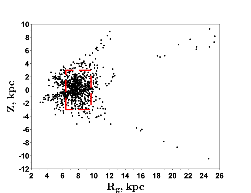
Figure 16: Distribution of RR Lyraes of our sample in the $R_{g}$-$Z$ coordinates. The red rectangle shows the domain of RR Lyraes selected for the $R_{g}$ and $Z$- clipped solution in Table 4

Table 4: Kinematical parameters and W1-band absolute-magnitude corrections of Galactic field RRLs from bimodal statistical parallax solution based on 533 field RRLs with close to solar Galactocentric distances ($6.4\leq R_{g}\leq 9.6$ kpc) located close to the Galactic plane ($|z|\leq 3.0$ kpc)) with bias correction based on 2500 simulated samples

Population	Fraction of the sample	$U_{0}$	$V_{0}$	$W_{0}$	$\sigma V_{R}$	$\sigma V_{\phi}$	$\sigma V_{\theta}$
	$\left(\alpha\right)$ & $\left(1-\alpha\right)$			$\left(kms^{-1}\right)$
Halo	0.763	-15.68	-218.62	-6.38	152.90	106.31	101.35
	$\pm 0.023$	$\pm 7.14$	$\pm 7.37$	$\pm 5.06$	$\pm 6.59$	$\pm 4.30$	$\pm 4.42$
Bias $\delta_{par}$	-0.001	-0.24	-0.37	-0.05	-0.14	-0.61	-0.19
	$\pm 0.001$	$\pm 0.15$	$\pm 0.15$	$\pm 0.10$	$\pm 0.13$	$\pm 0.09$	$\pm 0.08$
Bias corrected	0.762	-15.92	-218.99	-6.43	152.76	105.70	101.16
parameters	$\pm$ 0.022	$\pm$ 7.37	$\pm$ 5.06	$\pm$ 6.59	$\pm$ 4.30	$\pm$ 4.42	$\pm$ 4.61
Scatter(par)	0.022	7.49	7.49	5.11	6.28	4.71	4.19
Scatter(par)/$\sigma_{par}$	0.95	1.05	1.02	1.01	0.95	1.09	0.95
Disc	0.237	-19.05	-45.66	-14.01	49.07	38.62	25.45
	$\pm 0.023$	$\pm 5.19$	$\pm 4.92$	$\pm 2.69$	$\pm 4.46$	$\pm 3.93$	$\pm 2.54$
Bias $\delta_{par}$	+0.001	-0.15	-0.10	+0.01	-0.30	-0.25	-0.18
	$\pm 0.001$	$\pm 0.10$	$\pm 0.09$	$\pm 0.06$	$\pm 0.09$	$\pm 0.07$	$\pm 0.05$
Bias corrected	0.236	-19.20	-45.76	-14.00	48.77	38.37	25.27
parameters	$\pm$ 0.023	$\pm$ 5.19	$\pm$ 4.92	$\pm$ 2.69	$\pm$ 4.46	$\pm$ 3.93	$\pm$ 2.54
Scatter(par)	0.022	5.00	4.40	2.85	4.51	3.59	2.53
Scatter(par)/$\sigma_{par}$	0.95	0.96	0.89	1.06	1.01	0.91	1.00
$DeltaM$	-0.011$\pm$ 0.068
$\delta\Delta M$	-0.004$\pm$ 0.001
Bias corrected $\Delta M$	-0.015$\pm$ 0.068
$scatter_{\Delta M}$	0.068
$scatter_{\Delta M}$/$\sigma\Delta M$	1.00

As it is evident from Tables 3 and 4, the adopted maximum-likelihood statistical-parallax method yields practically bias-free results (the parameter biases never exceed 9% of the corresponding standard errors). Moreover, the error estimates also prove to be quite reliable as shown by the ratio of the scatter of the parameter values inferred for mock samples to the standard errors returned by the statistical-parallax method: these ratios are always contained in the interval from 0.89 to 1.06.

We thus adopt parameters given by the solution applied on the solar neighborhood sample (Table 4) as our final result. Examination of Table 4 shows that disk RRLs at close-to-solar Galacticentric distances rotate rapidly with small dispersion, ($V_{0}=187.2,\sigma V_{\phi}=38.4)$ km/s, while halo RRLs with close to solar $R_{g}$ rotate slowly with a large dispersion, ($V_{0}=14.0,\sigma V_{\phi}=105.7$) km/s, with respect to stationary Galactic center. These results agree with the estimates of Carollo et al. (2010) for the thick Disk ($V_{0}=182,\sigma V_{\phi}=51$)km/s and inner halo stars ($V_{0}=7,\sigma V_{\phi}=95$)km/s (see their table 5). Furthermore, our results are also consistent with a kinematically hot ($V/\sigma<<$1) halo and a kinematically cold ($V/\sigma\sim 1$) disk.

We also see that our result for halo RR Lyrae is strongly radially anisotropic ($\beta=0.54$) as suggested by Wegg et al. (2019) (see their fig 7, 8,9) form their study of the RRL kinematics as a tracer of inner Galactic halo using Gaia DR2. Our result of $\beta=0.54$ for solar-distance RRLs is less than the $\beta=0.7-0.8$ measured by Smith et al. (2009); Bond et al. (2010); Belokurov et al. (2018), but Belokurov et al. (2018) show that the local anisotropy of the stellar halo depends strongly on metallicity.

For comparison, we present in Table 5 the kinematic results of some previous statistical parallax studies for halo RRLs. As it is apparent from this table, our kinematic results for halo RRLs are in good agreement with previous works while providing a remarkable improvement in terms of errors and are more accurate and precise than any other study of this kind so far. The improvement in precision is due to the large number of RRLs used (as shown in the second column of Table 5) with accurate radial velocities and accurate Gaia DR2 proper motions, which translate into accurate tangential velocities when multiplied by the calibrated distance.

Table 5: Kinematic results of some previous statistical parallax studies for their halo RRLs

Reference	$N_{stars}$	$U_{0}$	$V_{0}$	$W_{0}$	$\sigma V_{R}$	$\sigma V_{\phi}$	$\sigma V_{\theta}$
Hawley et al. (1986)	77	21$\pm$19	-184$\pm$17	-4$\pm$11	166$\pm$76	114$\pm$52	91$\pm$40
Layden et al. (1996)	162	-9$\pm$14	-210$\pm$12	-12$\pm$8	168$\pm$13	102$\pm$8	97$\pm$7
Tsujimoto et al. (1997)	99	-12$\pm$17	-200$\pm$11	1$\pm$3	160$\pm$13	104$\pm$9	86$\pm$7
Dambis (2009)	364	-12$\pm$10	-217$\pm$9	-6$\pm$6	167$\pm$9	86$\pm$6	78$\pm$5
Dambis et al. (2013)	336	-7$\pm$9	-214$\pm$10	-10$\pm$6	153$\pm$9	101$\pm$6	96$\pm$5
This work	533	-16$\pm$7	-219$\pm$7	-6$\pm$5	153$\pm$7	106$\pm$4	101$\pm$4

4.2 Zero-point calibration of LZ and PLZ relations based on statistical parallax analysis

Our statistical parallax analysis of RRLs at close-to-solar Galactocentric distances and located within 3 kpc from the Galactic plane as described above yields an absolute magnitude correction of $\Delta M=-$0.015$\pm$0.068 (the last bold row of Table 4), and our final calibrated PLZ relation in the $W1$ band and on Zinn & West (1984) metallicity scale becomes

$$\begin{array}[]{rcl}\langle M_{W1}\rangle&=&-0.824(\pm 0.068)+0.124(\pm 0.023)[Fe/\\ &&H]-2.381(\pm 0.097)\log P_{F}\end{array}$$ (38)

The implied zero point correction for PLZ relation in Ks-band and for LZ relation in visual V-band results

$$\begin{array}[]{rcl}\langle M_{Ks}\rangle&=&-0.804(\pm 0.083)+0.101(\pm 0.027)[Fe/\\ &&H]-2.33\log P_{F}\\ \end{array}$$ (39)

and

$$\begin{array}[]{rcl}\langle M_{V}\rangle&=&1.041(\pm 0.077)+0.232(\pm 0.020)[Fe/H]\\ \end{array}$$ (40)

, respectively.

4.2.1 Comparison of PLZ and LZ relations with earlier works

In resent years, many different authors have calibrated the MIR WISE $W1$-band PLZ relation for RRLs both empirically (e.g. Dambis et al., 2013; Dambis et al., 2014; Sesar et al., 2017; Gaia Collaboration et al., 2017; Muraveva et al., 2018a) and theoretically (e.g Neeley et al., 2017). A brief summary of most of the previous studies are shown in table 3 of Muraveva et al. (2018b). According to these studies, the value of the period slope varies from $-2.247\pm 0.018$ (Neeley et al., 2017) to -2.470$\pm$0.074 (Sesar et al., 2017); the metallicity slope ranges from $0.088\pm 0.026$ (Dambis et al., 2013) to $0.18\pm 0.03$ (Neeley et al., 2017), and the zero point varies from $-0.79\pm 0.07$ (Neeley et al., 2017) to $-0.91\pm 0.36$ (Muraveva et al., 2018a).

All empirically estimated coefficients and zero points for the $W1$-band PLZ relation differ in the adopted metallicity scale and the zero point calibration methods, and this makes comparison of our results with those of other researchers difficult. Regardless of this, both our adopted coefficients and corrected zero point for W1-band PLZ relation marginally agree with all previous empirical and theoretical studies. However, our estimated metallicity is stepper than our previous measurement (Dambis et al., 2014) which had been made on single metallicity populations (i.e. in globular clusters). Moreover, our calibrated zero point is consistent with previous statistical parallax studies, and it is slightly brighter ($\sim 0.07$ mag) than the estimate obtained by Muraveva et al. (2018a) using other method.

The zero-point of our $M_{V}$-[Fe/H] relation at [Fe/H]=-1.5 ($M_{V}=+0.69\pm 0.08$) is consistent with all previous statistical parallax results (see Dambis et al., 2013, and references therein) except Kollmeier et al. (2013) ($M_{V,RRC}=+0.52\pm 0.11$ at $[Fe/H]=-1.59$ ), who calibrated LZ for RRC type variables. It is also consistent with the value of $M_{V}=0.65\pm 0.1$ mag obtained for the same metallicity by Muraveva et al. (2018a), who applied Bayesian approaches to 23 stars of our sample with homogeneous metallicity and Gaia DR2 parallaxes to model the LZ relation adopting the -0.057 mas parallax zero -point offset.

Like the visual $M_{V}-[Fe/H]$ relation, there is extensive literature on the NIR Ks- band PLZ relation for RRLs addressing it either from empirical (e.g see Gaia Collaboration et al., 2017; Neeley et al., 2019; Braga et al., 2018, and references therein) or theoretical (e.g. Bono et al., 2003; Catelan et al., 2004; Marconi et al., 2015) points of view. A comprehensive list of most of the published studies without the present ones are presented in table 3 of Muraveva et al. (2015). A glance at the coefficients listed in this table and the recent studies reveals the following features of the $Ks$- band PLZ relation of RRLs: the period slopes vary from -2.73 (Muraveva et al., 2015) to -2.101 (Bono et al., 2003); the metallicity slopes vary from 0.03 $\pm$ 0.07 (Muraveva et al., 2015) to 0.231$\pm$0.012(Bono et al., 2003); the zero points vary from from $-1.17\pm 0.1$ (Gaia Collaboration et al., 2017) to $-0.769\pm 0.088$ (Dambis et al., 2013), and all these coefficients depend on the metalicity scale and the zero point calibration method.

Our adopted period slope for Ks-band PLZ relation is consistent (within $1\sigma$ of uncertainties) with all previous empirical studies that uses Milky Way RRL samples and with Catelan et al. (2004) theoretical study. It also (within $2\sigma$ of uncertainties) with the previous empirical studies that uses LMC RRL sample (e.g. Borissova et al., 2009; Muraveva et al., 2015), but it is slightly shallower than the previous theoretical studies (e.g. Bono et al., 2003; Marconi et al., 2015). We obtained a significant metallicity dependence of absolute magnitudes in the $Ks$-band like theoretical studies (e.g. Bono et al., 2003; Catelan et al., 2004; Marconi et al., 2015) and the recent empirical studies (e.g. Muraveva et al., 2018a; Neeley et al., 2019; Braga et al., 2018) which was not the case in most of the previous empirical studies. The zero point of our calibrated Ks-band PLZ relation at $[Fe/H]=-1.5$ and period of P=0.5238d ($M_{Ks}=-0.30\pm 0.08$) is only slightly ($\sim$ 0.07 mag) fainter than the resent Muraveva et al. (2018a) calibration ($M_{Ks}=-0.37\pm 0.11$).

4.2.2 Comparison with Gaia DR2 parallax (Gaia DR2 zero-point offset)

A number of studies (eg. Gaia Collaboration et al., 2018b; Arenou et al., 2018; Gaia Collaboration et al., 2018a; Stassun & Torres, 2018; Riess et al., 2018; Zinn et al., 2018) confirmed that Gaia DR2 parallaxes have a systematic zero-point error, which depends on the type of object and on position in the sky. As an additional sanity check of our PLZ and LZ relations, we compared Gaia DR2 trigonometric parallaxes with photometric parallaxes inferred from our calibrated PLZ relation to estimate the zero-point offset for Gaia DR2 parallaxes. For the comparison, we selected 846 sample RRLs that have reliable trigonometric parallaxes from Gaia DR2 and then used our calibrated W1-band PLZ relation (equation 38) to estimate their photometric parallaxes.

Fig.17 compares our photometric parallaxes inferred from our calibrated W1-band PLZ relation and Gaia DR2 parallaxes for 846 RRLs. As expected, there is an overall systematic difference between the Gaia DR2 parallaxes and our photometric parallaxes which depends on magnitude. The non-weighted mean difference between Gaia DR2 and our photometric parallaxes is equal to $-0.065\pm 0.006$ mas. For comparison, in their validation of Gaia DR2 parallaxes for RR Lyrae stars, Arenou et al. (2018) find zero-point offsets of $-0.056\pm 0.005$ mas for RRLs in the Gaia DR2 catalogue and $-0.033\pm 0.009$ mas for RRLs in the GCVS.

Though, our estimated zero-point offset for Gaia DR2 parallax is slightly larger than the published estimates mentioned above, it agrees marginally, and this shows that Gaia DR2 astrometry has dramatically narrowed the gap between stasticall parallax and trigonometric parallax methods to find distance and absolute magnitude of RRLs that have been existing in the past studies before Gaia DR2.

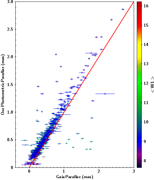
Figure 17: Comparison of the photometric parallaxes inferred from our calibrated $W1$-band PLZ relation with the corresponding DR2 parallaxes for 846 RRLs which have reliable estimates in both. The solid lines represent the bisectors and the auxiliary axis represent the W1-band mean magnitude.

4.3 Distance Measurements

In this section, we measure distances to the Galactic Center and LMC to check the performance of our calibrated PLZ and LZ relations.

4.3.1 Distance to the Galactic Center

Distance to the Galactic center ($R_{\odot}$) is important for the studies on the Galactic structure and dynamics. So far many authors have determined $R_{\odot}$ using different methods and different distance indicators. Here, we improve $R_{\odot}$ estimated by three authors using a similar procedure as Dambis et al. (2013). Thus, we use our calibrated PLZ or LZ relations (equation 38-39) for their Galactic bulge RRLs sample by taking $<[Fe/H]>=-1.0$ as an average metallicity for Galactic bulge RRLs (Walker & Terndrup, 1991) to rescale their $R_{\odot}$. Then, our best $R_{\odot}$ value is determined from the non weighted average of these three rescaled $R_{\odot}$.

The solar Galactocentric distance, $8.3\pm 1$ kpc, was inferred by Carney et al. (1995) using their $K$- band observations on the California Institute of Technology (CIT) system ($K_{\text{CIT}}$) for 58 RRLs in the Baade’s window and by adopting Jones et al. (1992) PL relations. Hence, in order to rescale this $R_{\odot}$ estimate using our PLZ relation in Ks-band (eq. 39) we first transformed our PLZ relation in Ks-band into $K_{\text{CIT}}$-band by ignoring the negligible and statistically insignificant coefficient of the colour term in the transformation equation :

$$\begin{array}[]{rcl}\langle M_{K,CIT}\rangle&=&-0.754(\pm 0.08)+0.082(\pm 0.026)\\ &&[Fe/H]_{ZW}-2.33)\log P_{F}\end{array}$$ (41)

It is noticeable that the zero-point of our $K_{\text{CIT}}$-band relation (eq. 41) in the Baade’s window becomes exactly equal to that of Jones et al. (1992) used by the above authors and hence we can leave the estimate obtained by Carney et al. (1995) unchanged, $R_{\odot}=(8.30\pm 1.0)$ kpc.

The $V$ band extinction corrected mean magnitude of RRLs in the Baade’s window, $<V_{0}>=15.44\pm 0.05$, was estimated by Collinge et al. (2006) from the Optical Gravitational Lensing Experiment (OGLE II) data. Using this result and our calibrated LZ relation (eq. 40) for the Baade’s window, we estimated the Galactic center distance module $\mu_{GC}=14.631\pm 0.128$ which corresponds to $R_{\odot}=8.44\pm 0.49$ kpc.

Groenewegen et al. (2008) also presented a catalog of 37 RRLs in the Galactic bulge that contains the dereddened $Ks$-band magnitudes and periods from their observations. This compilation without five bright outliers together with our calibrated PLZ relation in $Ks$-band at $<[Fe/H]>=-1.0$ offered Galactic center distance modulus estimate of $14.29\pm 0.1$  corresponding to $R_{\odot}$=7.21$\pm 0.62$  kpc.

Finally, we adopt the unweighted mean of our three $R_{\odot}$ measurement, $R_{\odot}=7.99\pm 0.48$, as our best $R_{\odot}$ estimate. This result is consistent with the result of Gravity Collaboration et al. (2019) ($R_{\odot}=8178\pm 13_{stat.}\pm 22_{sys.}pc$), which is estimated based on the orbital parameters of S2 star moving around the central massive black hole Sgr A^∗; but, it is less precise and shorter than the recent ones.

Our result for $R_{\odot}$ combined with the Reid & Brunthaler (2004) proper motion for the Sgr A^∗ along Galactic longitude( $\mu_{SgrA^{*}}$=6.379$\pm$0.026 mas yr^-1) implies a solar velocity of $-242\pm 15$ kms^-1. This is slightly smaller than the recent Hayes et al. (2018) estimate ($-253\pm 6$ kms^-1) using Gaia astrometry of Sagittarius Stream, but it agrees marginally. The estimated solar velocity is also consistent with the one ($\sim$ 238.1 km/s) that can be derived using the Oort constants calculated by Li et al. (2019) and the solar peculiar motion of Ding et al. (2019). This and our kinematic result in Table 4 lead us to conclude that both the inner halo and thick disk RRLs in the solar neighborhood undergoes a prograde rotation with a velocity of 23$\pm$17 kms^-1 and 196$\pm$16 kms^-1, respectively.

4.3.2 The Distance Modulus of the LMC

Another common distance measurement that can test our calibrated PLZ and LZ relations is the distance modulus of the LMC, whose value has been measured in countless studies using different distance indicators and independent techniques (see e.g. Gibson, 1999; Benedict et al., 2002; Clementini et al., 2003; De Grijs et al., 2014; Muraveva et al., 2018a, for compilation of the values in the literature).

In this paper, we measured the LMC distance modulus by applying our calibrated $Ks$-band PLZ relation (39) to a sample of 70 LMC RRLs compiled by Muraveva et al. (2015). For these 70 RRLs Muraveva et al. (2015) took the pulsation mode and periods from the OGLE III catalog (Soszynski et al., 2009) and photometry data from the VMC survey (Cioni et al., 2011) to estimate the $Ks$-band intensity-averaged magnitudes, and spectroscopic metallicities from Gratton et al. (2004), which are 0.06 dex more metal-rich than the Zinn & West (1984) scale. We used our calibrated $Ks$ band PLZ relation to determine the distance moduli for each of 70 LMC RRLs. We then computed the unweighted mean of the individual distance modulus estimates as the distance module of LMC, which is found to be 18.46$\pm$0.09. Our LMC distance modulus estimate agrees well with the most precise LMC distance module $18.477\pm 0.004_{(stat)}\pm 0.026_{(syst)}$ inferred by Pietrzyński et al. (2019) based on eclipsing binaries.

5 Conclusions

In this paper we compiled homogenized photometric (V-,Ks- and W1-band magnitudes), spectroscopic (radial velocity and metallicity) and astrometric (proper motions and parallaxes) data for a sample of 850 Galactic field RR Lyrae type variables. The compilation includes our new spectroscopic (for 448 RRLs) and photometric (for 251 RRLs ) observation data in addition to our previous compilation(Dambis et al., 2013) (for 402 RRLs). The astrometric data for all RRL samples are obtained from Gaia DR2. We used photometric data for a subsample of RRLs and Drimmel et al. (2003) 3D interstellar extinction model to calibrate the $(V-Ks)_{0}$ and $(V-W1)_{0}$ intrinsic colours of RRLs in terms of period and metallicity. Bimodal stastical parallax solutions for a subsample of RRLs with close-to-solar Galactocentric distances yields the zero point correction for our adopted LZ and PLZ relations, and the kinematical parameters for the halo and thick-disc RRL populations.

Our kinematical results indicate that the mean rotational velocity of the halo and disk RRLs in the solar neighborhood are 23$\pm$17 kms^-1 and 196$\pm$16 kms^-1, respectively, with respect to inertial Galactic center reference. Moreover, the velocity dispersions for both halo and disk RRL population are non-isotropic $(\sigma V_{R}>\sigma V_{\phi}>\sigma V_{\theta})$ in the solar neighborhood. Our kinematical results are in good agreement with previous statistical-parallax studies, but are considerably more accurate. Our currently largest homogeneous sample allowed us to reduce the uncertainty of RRLs distances down to $\sim+4.5\%$. Thus, our kinematic results represent the current best estimates of this kind of studies and are at the same time quite consistent with those obtained using other techniques.

Our calibrated LZ and PLZ relations also agree well with those reported in published studies based on statistical parallax analysis. However, the zero points of our calibrated relations are fainter ($\sim$0.1 mag) than other published estimates based on different methods. The reason for this is mostly due to underlying systematics in our analysis. Using our LZ and PLZ relations, we measured the solar Galactocentric distance ($R_{0}=7.99\pm 0.48$ kpc) and the LMC distance modulus (DM LMC = 18.46$\pm$0.09). Our $R_{0}$ estimate is in good agreement with the recent results using eclipsing binaries and our LMC distance modulus agrees within $\sim$0.04 mag with the current precise measurement of Pietrzyński et al. (2019). From the comparison of Gaia DR2 parallaxes with our photometric parallaxes that are estimated using our W1-band PLZ relation, we infer $-0.065\pm 0.006$ Gaia DR2 parallax offset. The magnitude of this offset is slightly larger than the published values.

Using our largest RRL database, we will investigate the structure and history of our Galaxy in near future by combining abundance analysis with kinematics. Further more, we will calibrate LZ and PLZ relations of RRLs using Bayesian Method. In the nearest future we expect to obtain more refined results concerning the kinematics and distance scale of Galactic RR Lyraes by expanding considerably the sample of these variables with 6D phase-space data provided by the recently published and forthcoming astrometric, photometric, and spectroscopic surveys and releases. These include primarily the next Gaia data releases (the third Gaia early data release with considerably improved per motions is expected by the end of 2020), PanStarrs and Zwicky Transient Factory optical photometric surveys, the available and forthcoming products based on the WISE mid-infrared space mission (unwise, catWISE, etc.), as well as extensive SDSS and LAMOST spectroscopic data.

Appendix A Some extra material

Additional Supporting Information may be found in the online version of this article: Table S1. The catalogue of observational data for 850 Galactic field RR Lyrae variables

References

- Anders et al. (2019) Anders F., et al., 2019, Astronomy & Astrophysics, 628, A94
- Arenou et al. (2018) Arenou F., et al., 2018, Astronomy & Astrophysics, 616, A17
- Barning (1963) Barning F. J., 1963, Bulletin of the Astronomical Institutes of the Netherlands, 17, 22
- Belokurov et al. (2018) Belokurov V., Erkal D., Evans N., Koposov S., Deason A., 2018, Monthly Notices of the Royal Astronomical Society, 478, 611
- Benedict et al. (2002) Benedict G. F., et al., 2002, The Astronomical Journal, 123, 473
- Berdnikov (1992) Berdnikov L., 1992, Soviet Astronomy Letters, 18, 207
- Berdnikov et al. (2012) Berdnikov L., Vozyakova O., Kniazev A. Y., Kravtsov V., Dambis A., Zhuiko S., 2012, Astronomy reports, 56, 290
- Berdnikov et al. (2017) Berdnikov L., Dagne T., Kniazev A., Dambis A., 2017, Information Bulletin on Variable Stars, 6212
- Bond et al. (2010) Bond N. A., et al., 2010, The Astrophysical Journal, 716, 1
- Bono et al. (2003) Bono G., Caputo F., Castellani V., Marconi M., Storm J., Degl’Innocenti S., 2003, Monthly Notices of the Royal Astronomical Society, 344, 1097
- Borissova et al. (2009) Borissova J., Rejkuba M., Minniti D., Catelan M., Ivanov V., 2009, Astronomy & Astrophysics, 502, 505
- Braga et al. (2018) Braga V., et al., 2018, The Astronomical Journal, 155, 137
- Buckley et al. (2006) Buckley D., Swart G., Meiring J., Stepp L., 2006, in Proc. SPIE.
- Burgh et al. (2003) Burgh E. B., Nordsieck K. H., Kobulnicky H. A., Williams T. B., O’Donoghue D., Smith M. P., Percival J. W., 2003, in Instrument Design and Performance for Optical/Infrared Ground-based Telescopes. pp 1463–1472
- Cacciari (2012) Cacciari C., 2012, Proceedings of the International Astronomical Union, 8, 101
- Cacciari et al. (1992) Cacciari C., Clementini G., Fernley J., 1992, The Astrophysical Journal, 396, 219
- Cardelli et al. (1989) Cardelli J. A., Clayton G. C., Mathis J. S., 1989, The Astrophysical Journal, 345, 245
- Carney et al. (1995) Carney B. W., Fulbright J. P., Terndrup D. M., Suntzeff N. B., Walker A. R., 1995, The Astronomical Journal, 110, 1674
- Carollo et al. (2010) Carollo D., et al., 2010, The Astrophysical Journal, 712, 692
- Carretta et al. (2009) Carretta E., Bragaglia A., Gratton R., D’Orazi V., Lucatello S., 2009, Astronomy & Astrophysics, 508, 695
- Catelan (2009) Catelan M., 2009, Astrophysics and Space Science, 320, 261
- Catelan et al. (2004) Catelan M., Pritzl B. J., Smith H. A., 2004, The Astrophysical Journal Supplement Series, 154, 633
- Chen et al. (2018a) Chen X., Wang S., Deng L., de Grijs R., Yang M., 2018a, The Astrophysical Journal Supplement Series, 237, 28
- Chen et al. (2018b) Chen B., et al., 2018b, Monthly Notices of the Royal Astronomical Society, 483, 4277
- Cioni et al. (2011) Cioni M.-R., et al., 2011, Astronomy & Astrophysics, 527, A116
- Clementini et al. (2003) Clementini G., Gratton R., Bragaglia A., Carretta E., Di Fabrizio L., Maio M., 2003, The Astronomical Journal, 125, 1309
- Clube & Dawe (1980) Clube S., Dawe J., 1980, Monthly Notices of the Royal Astronomical Society, 190, 591
- Collinge et al. (2006) Collinge M. J., Sumi T., Fabrycky D., 2006, The Astrophysical Journal, 651, 197
- Cousins (1976) Cousins A., 1976, Memoirs of the Royal Astronomical Society, 81, 25
- Crawford et al. (2010) Crawford S. M., et al., 2010, in Observatory Operations: Strategies, Processes, and Systems III. p. 773725
- Cutri et al. (2003) Cutri R., et al., 2003, " The IRSA 2MASS All-Sky Point Source Catalog, NASA/IPAC Infrared Science Archive. http://irsa. ipac. caltech. edu/applications/Gator/"
- Cutri et al. (2012) Cutri R., et al., 2012, VizieR On-line Data Catalog: II/311
- Cutri et al. (2013) Cutri R., et al., 2013, Explanatory Supplement to the AllWISE Data Release Products, by RM Cutri et al.
- Dagne et al. (2017) Dagne T., Berdnikov L., Kniazev A., Dambis A., 2017, Information Bulletin on Variable Stars, 63
- Dambis (2009) Dambis A. K., 2009, Monthly Notices of the Royal Astronomical Society, 396, 553
- Dambis & Rastorguev (2001) Dambis A., Rastorguev A., 2001, Astronomy Letters, 27, 108
- Dambis et al. (2013) Dambis A., Berdnikov L., Kniazev A. Y., Kravtsov V., Rastorguev A., Sefako R., Vozyakova O., 2013, Monthly Notices of the Royal Astronomical Society, 435, 3206
- Dambis et al. (2014) Dambis A., Rastorguev A., Zabolotskikh M., 2014, Monthly Notices of the Royal Astronomical Society, 439, 3765
- Dambis et al. (2017) Dambis A., Berdnikov L., Grebel E., Kniazev A., Katkov I., Dagne T., 2017, in EPJ Web of Conferences. p. 02007
- De Grijs et al. (2014) De Grijs R., Wicker J. E., Bono G., 2014, The Astronomical Journal, 147, 122
- Ding et al. (2019) Ding P.-J., Zhu Z., Liu J.-C., 2019, Research in Astronomy and Astrophysics, 19, 068
- Drimmel et al. (2003) Drimmel R., Cabrera-Lavers A., López-Corredoira M., 2003, Astronomy & Astrophysics, 409, 205
- Feast et al. (2008) Feast M. W., Laney C. D., Kinman T. D., Van Leeuwen F., Whitelock P. A., 2008, Monthly Notices of the Royal Astronomical Society, 386, 2115
- Federici et al. (2012) Federici L., Cacciari C., Bellazzini M., Fusi Pecci F., Galleti S., Perina S., 2012, A&A, 544, A155
- Fernley et al. (1993) Fernley J., Skillen I., Burki G., 1993, Astronomy and Astrophysics Supplement Series, 97, 815
- Fernley et al. (1998) Fernley J., Barnes T., Skillen I., Hawley S., Hanley C., Evans D., Solano E., Garrido R., 1998, Astronomy and Astrophysics, 330, 515
- Gavrilchenko et al. (2014) Gavrilchenko T., Klein C. R., Bloom J. S., Richards J. W., 2014, Monthly Notices of the Royal Astronomical Society, 441, 715
- Gibson (1999) Gibson B. K., 1999, arXiv preprint astro-ph/9910574
- Gould & Popowski (1998) Gould A., Popowski P., 1998, The Astrophysical Journal, 508, 844
- Gratton et al. (2004) Gratton R., Bragaglia A., Clementini G., Carretta E., Di Fabrizio L., Maio M., Taribello E., 2004, Astronomy & Astrophysics, 421, 937
- Groenewegen et al. (2008) Groenewegen M., Udalski A., Bono G., 2008, Astronomy & Astrophysics, 481, 441
- Hawley et al. (1986) Hawley S., Jefferys W., Barnes III T., Lai W., 1986, The Astrophysical Journal, 302, 626
- Hayes et al. (2018) Hayes C. R., Law D. R., Majewski S. R., 2018, The Astrophysical Journal Letters, 867, L20
- Hemenway (1975) Hemenway M., 1975, The Astronomical Journal, 80, 199
- Herk et al. (1965) Herk G. v., et al., 1965, Bulletin of the Astronomical Institutes of the Netherlands, 18, 71
- Hertzsprung (1919) Hertzsprung E., 1919, Astronomische Nachrichten, 210, 17
- Iben Jr (1974) Iben Jr I., 1974, Annual Review of Astronomy and Astrophysics, 12, 215
- Jones et al. (1992) Jones R. V., Carney B. W., Storm J., Latham D. W., 1992, The Astrophysical Journal, 386, 646
- Jones et al. (1996) Jones R. V., Carney B. W., Fulbright J. P., 1996, Publications of the Astronomical Society of the Pacific, 108, 877
- Kerr & Lynden-Bell (1986) Kerr F. J., Lynden-Bell D., 1986, Monthly Notices of the Royal Astronomical Society, 221, 1023
- Kinman et al. (2007) Kinman T., Cacciari C., Bragaglia A., Buzzoni A., Spagna A., 2007, Monthly Notices of the Royal Astronomical Society, 375, 1381
- Kinman et al. (2012) Kinman T., Cacciari C., Bragaglia A., Smart R., Spagna A., 2012, Monthly Notices of the Royal Astronomical Society, 422, 2116
- Kniazev et al. (2008) Kniazev A. Y., et al., 2008, Monthly Notices of the Royal Astronomical Society, 388, 1667
- Kniazev et al. (2019) Kniazev A. Y., Usenko I. A., Kovtyukh V. V., Berdnikov L. N., 2019, Astrophysical Bulletin, 74, 208
- Kobulnicky et al. (2003) Kobulnicky H. A., Nordsieck K. H., Burgh E. B., Smith M. P., Percival J. W., Williams T. B., O’Donoghue D., 2003, in Instrument Design and Performance for Optical/Infrared Ground-based Telescopes. pp 1634–1645
- Kochanek et al. (2017) Kochanek C., et al., 2017, Publications of the Astronomical Society of the Pacific, 129, 104502
- Koleva et al. (2009) Koleva M., Prugniel P., Bouchard A., Wu Y., 2009, Astronomy & Astrophysics, 501, 1269
- Kollmeier et al. (2013) Kollmeier J. A., et al., 2013, The Astrophysical Journal, 775, 57
- Layden (1998) Layden A. C., 1998, arXiv preprint astro-ph/9810461
- Layden et al. (1996) Layden A. C., Hanson R. B., Hawley S. L., Klemola A. R., Hanley C. J., 1996, arXiv preprint astro-ph/9608108
- Layden et al. (2019) Layden A. C., Tiede G. P., Chaboyer B., Bunner C., Smitka M. T., 2019, The Astronomical Journal, 158, 105
- Li et al. (2019) Li C., Zhao G., Yang C., 2019, The Astrophysical Journal, 872, 205
- Lindegren et al. (2018) Lindegren L., et al., 2018, arXiv preprint arXiv:1804.09366
- Lipka (2012) Lipka R., 2012, PhD thesis, University of Tasmania
- Liu (1991) Liu T., 1991, Publications of the Astronomical Society of the Pacific, 103, 205
- Lomb (1976) Lomb N. R., 1976, Astrophysics and space science, 39, 447
- Luo et al. (2012) Luo A.-L., et al., 2012, Research in Astronomy and Astrophysics, 12, 1243
- Luri et al. (1996) Luri X., Mennessier M., Torra J., Figueras F., 1996, Astronomy and Astrophysics Supplement Series, 117, 405
- Luri et al. (1998) Luri X., Gomez A., Torra J., Figueras F., Mennessier M., 1998, arXiv preprint astro-ph/9805215
- Madore et al. (2013) Madore B. F., et al., 2013, The Astrophysical Journal, 776, 135
- Maintz (2005) Maintz G., 2005, Astronomy & Astrophysics, 442, 381
- Marconi et al. (2015) Marconi M., et al., 2015, The Astrophysical Journal, 808, 50
- Mihalas & Binney (1981) Mihalas D., Binney J., 1981, San Francisco, CA, WH Freeman and Co., 1981. 608 p.
- Monson et al. (2017) Monson A. J., et al., 2017, The Astronomical Journal, 153, 96
- Muhie et al. (2020) Muhie T., Berdnikov L., Kniazev A., Dambis A., 2020, Variable Stars, 40
- Muraveva et al. (2015) Muraveva T., et al., 2015, The Astrophysical Journal, 807, 127
- Muraveva et al. (2018a) Muraveva T., Delgado H. E., Clementini G., Sarro L. M., Garofalo A., 2018a, arXiv preprint arXiv:1805.08742
- Muraveva et al. (2018b) Muraveva T., Garofalo A., Scowcroft V., Clementini G., Freedman W. L., Madore B. F., Monson A. J., 2018b, Monthly Notices of the Royal Astronomical Society, 480, 4138
- Neeley et al. (2017) Neeley J. R., et al., 2017, The Astrophysical Journal, 841, 84
- Neeley et al. (2019) Neeley J. R., et al., 2019, Monthly Notices of the Royal Astronomical Society, 490, 4254
- Nemec et al. (1994) Nemec J. M., Nemec A. F. L., Lutz T. E., 1994, The Astronomical Journal, 108, 222
- O’Donoghue et al. (2006) O’Donoghue D., et al., 2006, Monthly Notices of the Royal Astronomical Society, 372, 151
- Pancino et al. (2015) Pancino E., Britavskiy N., Romano D., Cacciari C., Mucciarelli A., Clementini G., 2015, Monthly Notices of the Royal Astronomical Society, 447, 2404
- Pavlovskaya (1953) Pavlovskaya E. D., 1953, Perem. Zvezdy, 9, 349
- Pietrzyński et al. (2019) Pietrzyński G., et al., 2019, Nature, 567, 200
- Pojmanski (2002) Pojmanski G., 2002, arXiv preprint astro-ph/0210283
- Popowski & Gould (1998) Popowski P., Gould A., 1998, The Astrophysical Journal, 506, 271
- Prugniel et al. (2011) Prugniel P., Vauglin I., Koleva M., 2011, Astronomy & Astrophysics, 531, A165
- Pshenichnyi & Redkovskii (1976) Pshenichnyi B., Redkovskii N., 1976, Zhurnal Vychislitel’noi Matematiki i Matematicheskoi Fiziki, 16, 1388
- Reid & Brunthaler (2004) Reid M. J., Brunthaler A., 2004, The Astrophysical Journal, 616, 872
- Riess et al. (2018) Riess A. G., et al., 2018, The Astrophysical Journal, 861, 126
- Rigal (1958) Rigal J. L., 1958, Bull. Astron. Paris, 22, 22, 171
- Salaris & Cassisi (2005) Salaris M., Cassisi S., 2005, Evolution of stars and stellar populations. John Wiley & Sons
- Samus et al. (2012) Samus N. N., Durlevich O. V., Kazarovets E. V., Kireeva N. N., Pastukhova E. N., Zharova A. V., et al. 2012, VizieR On-line Data Catalog, p. 1
- Samus et al. (2017) Samus N., Kazarovets E., Durlevich O., Kireeva N., Pastukhova E., et al., 2017, Astronomy Reports, 61, 80
- Sartoretti et al. (2018) Sartoretti P., et al., 2018, Astronomy & Astrophysics, 616, A6
- Scargle (1982) Scargle J. D., 1982, The Astrophysical Journal, 263, 835
- Sesar et al. (2017) Sesar B., Fouesneau M., Price-Whelan A. M., Bailer-Jones C. A., Gould A., Rix H.-W., 2017, The Astrophysical Journal, 838, 107
- Skillen et al. (1993) Skillen I., Fernley J., Stobie R., Jameson R., 1993, Monthly Notices of the Royal Astronomical Society, 265, 301
- Skrutskie et al. (2006) Skrutskie M., et al., 2006, The Astronomical Journal, 131, 1163
- Smith (1995) Smith H., 1995, RR Lyrae Stars (Cambridge
- Smith et al. (2009) Smith M. e. a., et al., 2009, Monthly Notices of the Royal Astronomical Society, 399, 1223
- Soszynski et al. (2009) Soszynski I., et al., 2009, arXiv preprint arXiv:0910.1354
- Stassun & Torres (2018) Stassun K. G., Torres G., 2018, The Astrophysical Journal, 862, 61
- Strugnell et al. (1986) Strugnell P., Reid N., Murray C., 1986, Monthly Notices of the Royal Astronomical Society, 220, 413
- Tsujimoto et al. (1997) Tsujimoto T., Miyamoto M., Yoshii Y., 1997, The Astrophysical Journal Letters, 492, L79
- Walker & Terndrup (1991) Walker A. R., Terndrup D. M., 1991, The Astrophysical Journal, 378, 119
- Wegg et al. (2019) Wegg C., Gerhard O., Bieth M., 2019, Monthly Notices of the Royal Astronomical Society, 485, 3296
- Wright et al. (2010) Wright E. L., et al., 2010, The Astronomical Journal, 140, 1868
- Yuan et al. (2013) Yuan H.-B., Liu X.-W., Xiang M.-S., 2013, Monthly Notices of the Royal Astronomical Society, 430, 2188
- Zinn & West (1984) Zinn R., West M. J., 1984, The Astrophysical Journal Supplement Series, 55, 45
- Zinn et al. (2018) Zinn J. C., Pinsonneault M. H., Huber D., Stello D., 2018, arXiv preprint arXiv:1805.02650
- Gaia Collaboration et al. (2017) Gaia Collaboration et al., 2017, Astronomy & Astrophysics, 605, A79
- Gaia Collaboration et al. (2018a) Gaia Collaboration et al., 2018a, Astronomy & Astrophysics, 616, A9
- Gaia Collaboration et al. (2018b) Gaia Collaboration et al., 2018b, Astronomy & Astrophysics, 616
- Gaia Collaboration et al. (2019) Gaia Collaboration et al., 2019, Astronomy & Astrophysics, 622, A60
- Gravity Collaboration et al. (2019) Gravity Collaboration et al., 2019, Astronomy & Astrophysics, 625, L10