VECoDeR - Variational Embeddings for Community Detection and Node Representation

Abstract

In this paper, we study how to simultaneously learn two highly correlated tasks of graph analysis, i.e., community detection and node representation learning. We propose an efficient generative model called VECoDeR for jointly learning Variational Embeddings for Community Detection and node Representation. VECoDeR assumes that every node can be a member of one or more communities. The node embeddings are learned in such a way that connected nodes are not only “closer” to each other but also share similar community assignments. A joint learning framework leverages community-aware node embeddings for better community detection. We demonstrate on several graph datasets that VECoDeR effectively outperforms many competitive baselines on all three tasks i.e. node classification, overlapping community detection and non-overlapping community detection. We also show that VECoDeR is computationally efficient and has quite robust performance with varying hyperparameters.

1 Introduction

Graphs are flexible data structures that model complex relationships among entities, i.e. data points as nodes and the relations between nodes via edges. One important task in graph analysis is community detection, where the objective is to cluster nodes into multiple groups (communities). Each community is a set of densely connected nodes. The communities can be overlapping or non-overlapping, depending on whether they share some nodes or not. Several algorithmic (Ahn et al., 2010; Derényi et al., 2005) and probabilistic approaches (Gopalan and Blei, 2013; Leskovec and Mcauley, 2012; Wang et al., 2017; Yang et al., 2013) to community detection have been proposed. Another fundamental task in graph analysis is learning the node embeddings. These embeddings can then be used for downstream tasks like graph visualization (Tang et al., 2016; Wang et al., 2016; Gao et al., 2011; Wang et al., 2017) and classification (Cao et al., 2015; Tang et al., 2015).

In the literature, these tasks are usually treated separately. Although the standard graph embedding methods capture the basic connectivity, the learning of the node embeddings is independent of community detection. For instance, a simple approach can be to get the node embeddings via DeepWalk (Perozzi et al., 2014) and get community assignments for each node by using k-means or Gaussian mixture model. Looking from the other perspective, methods like Bigclam (Yang and Leskovec (2013)), that focus on finding the community structure in the dataset, perform poorly for node-representation tasks e.g. node classification. This motivates us to study the approaches that jointly learn community-aware node embeddings.

Recently several approaches, like CNRL (Tu et al., 2018), ComE (Cavallari et al., 2017), vGraph (Sun et al. (2019)) etc, have been proposed to learn the node embeddings and detect communities simultaneously in a unified framework. Several studies have shown that community detection is improved by incorporating the node representation in the learning process (Cao et al., 2015; Kozdoba and Mannor, 2015). The intuition is that the global structure of graphs learned during community detection can provide useful context for node embeddings and vice versa.

The joint learning methods (CNRL, ComE and vGraph) learn two embeddings for each node. One node embedding is used for the node representation task. The second node embedding is the “context” embedding of the node which aids in community detection. As CNRL and ComE are based on Skip-Gram (Mikolov et al., 2013) and DeepWalk (Perozzi et al., 2014), they inherit “context” embedding from it for learning the neighbourhood information of the node. vGraph also requires two node embeddings for parameterizing two different distributions. In contrast, we propose learning a single community-aware node representation which is directly used for both tasks. In this way, we not only get rid of an extraneous node embedding but also reduce the computational cost.

In this paper, we propose an efficient generative model called VECoDeR for jointly learning both community detection and node representation. The underlying intuition behind VECoDeR is that every node can be a member of one or more communities. However, the node embeddings should be learned in such a way that connected nodes are “closer” to each other than unconnected nodes. Moreover, connected nodes should have similar community assignments. Formally, we assume that for $i$-th node, the node embeddings ${\bm{z}}_{i}$ are generated from a prior distribution $p({\bm{z}})$. Given ${\bm{z}}_{i}$, the community assignments $c_{i}$ are sampled from $p(c_{i}|{\bm{z}}_{i})$, which is parameterized by node and community embeddings. In order to generate an edge $(i,j)$, we sample another node embedding ${\bm{z}}_{j}$ from $p({\bm{z}})$ and respective community assignment $c_{j}$ from $p(c_{j}|{\bm{z}}_{j})$. Afterwards, the node embeddings and the respective community assignments of node pairs are fed to a decoder. The decoder ensures that embeddings of both the nodes and the communities of connected nodes share high similarity. This enables learning such node embeddings that are useful for both community detection and node representation tasks.

We validate the effectiveness of our approach on several real-world graph datasets. In Sec. 4, we show empirically that VECoDeR is able to outperform the baseline methods including the direct competitors on all three tasks i.e. node classification, overlapping community detection and non-overlapping community detection. Furthermore, we compare the computational cost of training different algorithms. VECoDeR is up to 40x more time-efficient than its competitors. We also conduct hyperparameter sensitivity analysis which demonstrates the robustness of our approach. Our main contributions are summarized below:

• We propose an efficient generative model called VECoDeR for joint community detection and node representation learning.

• We adopt a novel approach and argue that a single node embedding is sufficient for learning both the representation of the node itself and its context.

• Training VECoDeR is extremely time-efficient in comparison to its competitors.

2 Related Work

Community Detection. Early community detection algorithms are inspired from clustering algorithms (Xie et al., 2013). For instance, spectral clustering (Tang and Liu, 2011) is applied to the graph Laplacian matrix for extracting the communities. Similarly, several matrix factorization based methods have been proposed to tackle the community detection problem. For example, Bigclam (Yang and Leskovec (2013)) treats the problem as a non-negative matrix factorization (NMF) task. It aims to recover the node-community affiliation matrix and learns the latent factors which represent community affiliations of nodes. Another method CESNA(Yang et al. (2013)) extends Bigclam by modelling the interaction between the network structure and the node attributes. The performance of matrix factorization methods is limited due to the capacity of the bi-linear models. Some generative models, like vGraph (Sun et al., 2019), Circles (Leskovec and Mcauley (2012)) etc, have also been proposed to detect communities in a graph.

Node Representation Learning. Many successful algorithms which learn node representation in an unsupervised way are based on random walk objectives (Perozzi et al., 2014; Tang et al., 2015; Grover and Leskovec, 2016; Hamilton et al., 2017). Some known issues with random-walk based methods (e.g. DeepWalk, node2vec etc) are: (1) They sacrifice the structural information of the graph by putting over-emphasis on the proximity information (Ribeiro et al., 2017) and (2) great dependence of the performance on hyperparameters (walk-length, number of hops etc) (Perozzi et al., 2014; Grover and Leskovec, 2016). Recently, Gilmer et al. (2017) recently showed that graph convolutions encoder models greatly reduce the need for using the random-walk based training objectives. This is because the graph convolutions enforce that the neighboring nodes have similar representations. Some interesting GCN based approaches include graph autoencoders e.g. GAE and VGAE(Kipf and Welling (2016b)) and DGI(Velickovic et al., 2019).

Joint community detection and node representation learning. In the literature, several attempts have been made to tackle both these tasks in a single framework. Most of these methods propose an alternate optimization process, i.e. learn node embeddings and improve community assignments with them and vice versa (Cavallari et al., 2017; Tu et al., 2018). Some approaches, like CNRL (Tu et al., 2018) and ComE (Cavallari et al., 2017), are inspired from random walk, thus inheriting the shortcomings of random walk. Others, like GEMSEC (Rozemberczki et al. (2019), are limited to the detection of non-overlapping communities. There also exist some generative models like CommunityGAN (Jia et al. (2019)) and vGraph (Sun et al. (2019)) that jointly learn community assignments and node embeddings. Some methods have high computational complexity, i.e. quadratic to the number of nodes in a graph, e.g. M-NMF (Wang et al. (2017)) and DNR (Yang et al., 2016a). CNRL, ComE and vGraph require learning two embeddings for each node for simultaneously tackling the two tasks. Unlike them, VECoDeR learns a single community-aware node representation which is directly used for both tasks.

It is pertinent to highlight that although both vGraph and VECoDeR adopt a variational approach but the underlying models are quite different. vGraph assumes that each node can be represented as a mixture of multiple communities and is described by a multinomial distribution over communities, whereas VECoDeR models the node embedding by a single distribution. For a given node, vGraph, first draws a community assignment and then a connected neighbor node is generated based on the assignment. Whereas, VECoDeR draws the node embedding from prior distribution and then community assignment is conditioned on a single node only. In simple terms, vGraph also needs edge information in the generative process whereas VECoDeR does not require it. VECoDeR relies on the decoder to ensure that embeddings of the connected nodes and their communities share high similarity with each other.

3 Methodology

3.1 Problem Formulation

Suppose an undirected graph ${\mathcal{G}}=({\mathcal{V}},{\mathcal{E}})$ with the adjacency matrix ${\bm{A}}\in{\mathbb{R}}^{N\times N}$ and a matrix ${\bm{X}}\in{\mathbb{R}}^{N\times F}$ of $F$-dimensional node features, $N$ being the number of nodes. Given $K$ as the number of communities, we aim to jointly learn the node embeddings and the community embeddings following a variational approach such that: (1) One or more communities can be assigned to every node and (2) the node embeddings can be used for both community detection and node classification.

3.2 Variational Model

Generative Model: Let us denote the latent node embedding and community assignment for $i$-th node by the random variables ${\bm{z}}_{i}\in\mathbb{R}^{d}$ and $c_{i}$ respectively. The generative model is given by:

$$p({\bm{A}})=\int\sum\limits_{{\bm{c}}}p({\bm{Z}},{\bm{c}},{\bm{A}})d{\bm{Z}},$$ (1)

where ${\bm{c}}=[c_{1},c_{2},\cdots,c_{N}]$ and the matrix ${\bm{Z}}=[{\bm{z}}_{1},{\bm{z}}_{2},\cdots,{\bm{z}}_{N}]$ stacks the node embeddings. The joint distribution in (1) is mathematically expressed as

$$p({\bm{Z}},{\bm{c}},{\bm{A}})=p({\bm{Z}})\ p_{\theta}({\bm{c}}|{\bm{Z}})\ p_{\theta}({\bm{A}}|{\bm{c}},{\bm{Z}}),$$ (2)

where $\theta$ denotes the model parameters. Let us denote elements of ${\bm{A}}$ by $a_{ij}$. Following existing approaches (Kipf and Welling, 2016b; Khan et al., 2020), we consider ${\bm{z}}_{i}$ to be $i.i.d$ random variables. Furthermore, assuming $c_{i}|{\bm{z}}_{i}$ to be $i.i.d$ random variables, the joint distributions in (2) can be factorized as

$$p({\bm{Z}}) =\prod\limits_{i=1}^{N}p({\bm{z}}_{i})$$ (3)

$$p_{\theta}({\bm{c}}|{\bm{Z}}) =\prod\limits_{i=1}^{N}p_{\theta}(c_{i}|{\bm{z}}_{i})$$ (4)

$$p_{\theta}({\bm{A}}|{\bm{c}},{\bm{Z}}) =\prod\limits_{i,j}p_{\theta}(a_{ij}|c_{i},c_{j},{\bm{z}}_{i},{\bm{z}}_{j}),$$ (5)

where Eq. (5) assumes that the edge decoder $p_{\theta}(a_{ij}|c_{i},c_{j},{\bm{z}}_{i},{\bm{z}}_{j})$ depends only on $c_{i},c_{j},{\bm{z}}_{i}$ and ${\bm{z}}_{j}$.

Inference Model: We aim to learn the model parameters $\theta$ such that $\text{log}(p_{\theta}({\bm{A}}))$ is maximized. In order to ensure computational tractability, we introduce the approximate posterior

$$q_{\phi}({\bm{Z}},{\bm{c}}|{\mathcal{I}}) =\prod\limits_{i}q_{\phi}({\bm{z}}_{i},c_{i}|{\mathcal{I}})$$ (6)

$$=\prod\limits_{i}q_{\phi}({\bm{z}}_{i}|{\mathcal{I}})q_{\phi}(c_{i}|{\bm{z}}_{i},{\mathcal{I}}),$$ (7)

where ${\mathcal{I}}=({\bm{A}},{\bm{X}})$ if node features are available, otherwise ${\mathcal{I}}={\bm{A}}$. We maximize the corresponding ELBO bound (for derivation, refer to the supplementary material), given by

$$\mathcal{L}_{\mathrm{ELBO}}\approx -\sum\limits_{i=1}^{N}D_{KL}(q_{\phi}({\bm{z}}_{i}|{\mathcal{I}})\ ||\ p({\bm{z}}_{i}))$$

$$- \sum\limits_{i=1}^{N}\frac{1}{M}\sum\limits_{m=1}^{M}D_{KL}(q_{\phi}(c_{i}|{\bm{z}}_{i}^{(m)},{\mathcal{I}})\ ||\ p_{\theta}(c_{i}|{\bm{z}}_{i}^{(m)}))$$

$$+ \sum\limits_{(i,j)\in{\mathcal{E}}}\mathbb{E}_{({\bm{z}}_{i},{\bm{z}}_{j},c_{i},c_{j})\sim q_{\phi}({\bm{z}}_{i},{\bm{z}}_{j},c_{i},c_{j}|{\mathcal{I}})}\bigg{\{}$$

$$\text{log}\bigg{(}p_{\theta}(a_{ij}|c_{i},c_{j},{\bm{z}}_{i},{\bm{z}}_{j})\bigg{)}\bigg{\}},$$ (8)

where $D_{KL}(.||.)$ represents the KL-divergence between two distributions. The distribution $q_{\phi}({\bm{z}}_{i},{\bm{z}}_{j},c_{i},c_{j}|{\mathcal{I}})$ in the third term of Eq. (8) is factorized into two conditionally independent distributions i.e.

$$q_{\phi}({\bm{z}}_{i},{\bm{z}}_{j},c_{i},c_{j}|{\mathcal{I}})=q_{\phi}({\bm{z}}_{i},c_{i}|{\mathcal{I}})q_{\phi}({\bm{z}}_{j},c_{j}|{\mathcal{I}}).$$ (9)

3.3 Design Choices

In Eq. (3), $p({\bm{z}}_{i})$ is chosen to be the standard gaussian distribution for all $i$. The corresponding approximate posterior $q_{\phi}({\bm{z}}_{i}|{\mathcal{I}})$ in Eq. (7), used as node embeddings encoder, is given by

$$q_{\phi}({\bm{z}}_{i}|{\mathcal{I}})={\mathcal{N}}\big{(}\bm{\mu}_{i}({\mathcal{I}}),\text{diag}({\bm{\sigma}^{2}}_{i}({\mathcal{I}}))\big{)}.$$ (10)

The parameters of $q_{\phi}({\bm{z}}_{i}|{\mathcal{I}})$ can be learnt by any encoder network e.g. graph convolutional network (Kipf and Welling (2016a)), graph attention network ( Veličković et al. (2017)), GraphSAGE (Hamilton et al. (2017)) or even two matrices to learn $\bm{\mu}_{i}({\mathcal{I}})$ and $\text{diag}({\bm{\sigma}^{2}}_{i}({\mathcal{I}}))$. Samples are then generated using reparametrization trick (Doersch (2016)).

For parameterizing $p_{\theta}(c_{i}|{\bm{z}}_{i})$ in Eq. (4), we introduce community embeddings $\{{\bm{g}}_{1},\cdots,{\bm{g}}_{K}\};\ {\bm{g}}_{k}\in\mathbb{R}^{d}$. The distribution $p_{\theta}(c_{i}|{\bm{z}}_{i})$ is then modelled as the softmax of dot products of ${\bm{z}}_{i}$ with ${\bm{g}}_{k}$, i.e.

$$p_{\theta}(c_{i} =k|{\bm{z}}_{i})=\frac{\text{exp}(<{\bm{z}}_{i},{\bm{g}}_{k}>)}{\sum\limits_{\ell=1}^{K}\text{exp}(<{\bm{z}}_{i},{\bm{g}}_{\ell}>)}.$$ (11)

The corresponding approximate posterior $q_{\phi}(c_{i}=k|{\bm{z}}_{i},{\mathcal{I}})$ in Eq. (7) is affected by the node embedding ${\bm{z}}_{i}$ as well as the neighborhood. To design this, our intuition is to consider the similarity of ${\bm{g}}_{k}$ with the embedding ${\bm{z}}_{i}$ as well as with the embeddings of the neighbors of the $i$-th node. The overall similarity with neighbors is mathematically formulated as the average of the dot products of their embeddings. Afterwards, a hyperparameter $\alpha$ is introduced to control the bias between the effect of ${\bm{z}}_{i}$ and the set ${\mathcal{N}}_{i}$ of the neighbors of the $i$-th node. Finally, a softmax is applied, i.e.

$$q_{\phi}(c_{i}=k|{\bm{z}}_{i},{\mathcal{G}}) =\mathrm{softmax}\Big{(}\alpha<{\bm{z}}_{i},{\bm{g}}_{k}>$$

$$+(1-\alpha)\frac{1}{|{\mathcal{N}}_{i}|}\sum\limits_{j\in{\mathcal{N}}_{i}}<{\bm{z}}_{j},{\bm{g}}_{k}>\Big{)}\Big{)}.$$ (12)

Hence, Eq. (12) ensures that graph structure information is employed to learn community assignments instead of relying on an extraneous node embedding as done in (Sun et al., 2019; Cavallari et al., 2017). Finally, the choice of edge decoder in Eq. (5) is motivated by the intuition that the nodes connected by edges have a high probability of belonging to the same community and vice versa. Therefore we model the edge decoder as:

$$p_{\theta}(a_{ij}|c_{i} =\ell,c_{j}=m,{\bm{z}}_{i},{\bm{z}}_{j})$$

$$=\frac{\sigma(<{\bm{z}}_{i},{\bm{g}}_{m}>)+\sigma(<{\bm{z}}_{j},{\bm{g}}_{\ell}>)}{2}.$$ (13)

For better reconstructing the edges, Eq. (13) makes use of the community embeddings, node embeddings and community assignment information simultaneously. This helps in learning better node representations by leveraging the global information about the graph structure via community detection. On the other hand, this also forces the community assignment information to exploit the local graph structure via node embeddings and edge information.

3.4 Practical Aspects

The third term in Eq. (8) is estimated in practice using the samples generated by the approximate posterior. This term is equivalent to the negative of binary cross-entropy (BCE) loss between observed edges and reconstructed edges. Since community assignment follows a categorical distribution, we use Gumbel-softmax (Jang et al. (2016)) for backpropagation of the gradients. As for the second term of Eq. (8), it is also enough to set $M=1$, i.e. use only one sample per input node.

For inference, non-overlapping community assignment can be obtained for $i$-th node as

$${\mathcal{C}}_{i}=\operatorname*{arg\,max}\limits_{k\in\{1,\cdots,K\}}\ q_{\phi}(c_{i}=k|{\bm{z}}_{i},{\mathcal{I}}).$$ (14)

To get overlapping community assignments for $i$-th node, we can threshold its weighted probability vector at $\epsilon$, a hyperparameter, as follows

$${\mathcal{C}}_{i}=\Big{\{}k\ \bigg{\rvert}\ \frac{q_{\phi}(c_{i}=k|{\bm{z}}_{i},{\mathcal{I}})}{\max\limits_{\ell}q_{\phi}(c_{i}=\ell|{\bm{z}}_{i},{\mathcal{I}})}\geq\epsilon\Big{\}},\quad\epsilon\in[0,1].$$ (15)

3.5 Complexity

Computation of dot products for all combinations of node and community embeddings takes ${\mathcal{O}}(NKd)$ time. Solving Eq. (12) further requires calculation of mean of dot products over the neighborhood for every node, which takes ${\mathcal{O}}(|{\mathcal{E}}|K)$ computations overall as we traverse every edge for every community. Finally, we need softmax over all communities for every node in Eq. (11) and Eq. (12) which takes ${\mathcal{O}}(NK)$ time. Eq. (13) takes ${\mathcal{O}}(|{\mathcal{E}}|)$ time for all edges as we have already calculated the dot products. As a result, the overall complexity becomes ${\mathcal{O}}(|{\mathcal{E}}|K+NKd)$. This complexity is quite low compared to other algorithms designed to achieve similar goals (Cavallari et al., 2017; Wang et al., 2017; Yang et al., 2016a).

Dataset	$|{\mathcal{V}}|$	$|{\mathcal{E}}|$	$K$	$|F|$	Overlap
CiteSeer	3327	9104	6	3703	N
CiteSeer-full	4230	10674	6	602	N
Cora	2708	10556	7	1433	N
Cora-ML	2995	16316	7	2879	N
Cora-full	19793	126842	70	8710	N
fb0	333	2519	24	N/A	Y
fb107	1034	26749	9	N/A	Y
fb1684	786	14024	17	N/A	Y
fb1912	747	30025	46	N/A	Y
fb3437	534	4813	32	N/A	Y
fb348	224	3192	14	N/A	Y
fb414	150	1693	7	N/A	Y
fb698	61	270	13	N/A	Y
youtube	5346	24121	5	N/A	Y
amazon	794	2109	5	N/A	Y
amazon500	1113	3496	500	N/A	Y
amazon1000	1540	4488	1000	N/A	Y
dblp	24493	89063	5	N/A	Y

Table 1: Every dataset has $|{\mathcal{V}}|$ nodes, $|{\mathcal{E}}|$ edges, $K$ communities and $|F|$ features. $|F|=\text{N/A}$ means that either the features were missing or not used.

4 Experiments

4.1 Datasets

We have selected 18 different datasets ranging from 270 to 126,842 edges. For non-overlapping community detection and node classification, we use 5 the citation datasets (Bojchevski and Günnemann (2017); Yang et al. (2016b)). The remaining datasets (Leskovec and Mcauley (2012); Yang and Leskovec (2015)), used for overlapping community detection, are taken from SNAP repository (Leskovec and Krevl (2014)). Following (Sun et al., 2019), we take 5 biggest ground truth communities for youtube, amazon and dblp. Moreover, we also analyse the case of large number of communities. For this purpose, we prepare two subsets of amazon dataset by randomly selecting 500 and 1000 communities from 2000 smallest communities in the amazon dataset.

4.2 Baselines

For overlapping community detection, we compare with the following competitive baselines: MNMF(Wang et al., 2017) learns community membership distribution by using joint non-negative matrix factorization with modularity based regularization. BIGCLAM(Yang and Leskovec (2013)) also formulates community detection as a non-negative matrix factorization (NMF) task. It simultaneously optimizes the model likelihood of observed links and learns the latent factors which represent community affiliations of nodes. CESNA (Yang et al. (2013)) extends BIGCLAM by statistically modelling the interaction between the network structure and the node attributes. Circles (Leskovec and Mcauley (2012)) introduces a generative model for community detection in ego-networks by learning node similarity metrics for every community. SVI (Gopalan and Blei (2013)) formulates membership of nodes in multiple communities by a Bayesian model of networks. vGraph (Sun et al. (2019)) simultaneously learns node embeddings and community assignments by modelling the nodes as being generated from a mixture of communities. vGraph+, a variant further incorporates regularization to weigh local connectivity. ComE (Cavallari et al. (2017)) jointly learns community and node embeddings by using gaussian mixture model formulation. CNRL(Tu et al., 2018) enhances the random walk sequences (generated by DeepWalk, node2vec etc) to jointly learn community and node embeddings. CommunityGAN (ComGAN)is a generative adversarial model for learning node embeddings such that the entries of the embedding vector of each node refer to the membership strength of the node to different communities. Lastly, we compare the results with the communities obtained by applying k-means to the learned embeddings of DGI (Velickovic et al., 2019).

For non-overlapping community detection and node classification, in addition to MNMF, DGI, CNRL, CommunityGAN, vGraph and ComE, we compare VECoDeR with the following baselines: DeepWalk (Perozzi et al. (2014)) makes use of SkipGram (Mikolov et al. (2013)) and truncated random walks on network to learn node embeddings. LINE (Tang et al. (2015)) learns node embeddings while attempting to preserve first and second order proximities of nodes. Node2Vec (Grover and Leskovec (2016)) learns the embeddings using biased random walk while aiming to preserve network neighborhoods of nodes. Graph Autoencoder (GAE)Kipf and Welling (2016b) extends the idea of autoencoders to graph datasets. We also include its variational counterpart i.e. VGAE. GEMSEC is a sequence sampling-based learning model which aims to jointly learn the node embeddings and clustering assignments.

4.3 Settings

For overlapping community detection, we learn mean and log-variance matrices of 16-dimensional node embeddings. We set $\alpha=0.9$ and $\epsilon=0.3$ in all our experiments. Following Kipf and Welling (2016b), we first pre-train a variational graph autoencoder. We perform gradient descent with Adam optimizer (Kingma and Ba (2014)) and learning rate $=0.01$. Community assignments are obtained using Eq. (15). For the baselines, we employ the results reported by Sun et al. (2019). For evaluating the performance, we use F1-score and Jaccard similarity.

For non-overlapping community detection, since the default implementations of most the baselines use $128$ dimensional embeddings, for we use $d=128$ for fair comparison. Eq. (14) is used for community assignments. For vGraph, we use the code provided by the authors. We employ normalized mutual information (NMI) and adjusted random index (ARI) as evaluation metrics.

For node classification, we follow the training split used in various previous works (Yang et al., 2016b; Kipf and Welling, 2016a; Velickovic et al., 2019), i.e. $20$ nodes per class for training. We train logistic regression using LIBLINEAR (Fan et al. (2008)) solver as our classifier and report the evaluation results on rest of the nodes. For the algorithms that do not use node features, we train the classifier by appending the raw node features with the learnt embeddings. For evaluation, we use F1-macro and F1-micro scores.

All the reported results are the average over five runs. Further implementation details can be found in the code: https://github.com/RayyanRiaz/vecoder.

F1 Score (%)
Dataset	MNMF	Bigclam	CESNA	Circles	SVI	vGraph	vGraph+	ComE	CNRL	ComGan	DGI	VECoDeR
fb0	14.4	29.5	28.1	28.6	28.1	24.4	26.1	31.1	11.5	35.0	27.35	34.7
fb107	12.6	39.3	37.3	24.7	26.9	28.2	31.8	39.7	20.2	47.5	35.78	59.7
fb1684	12.2	50.4	51.2	28.9	35.9	42.3	43.8	52.9	38.5	47.6	42.85	56.4
fb1912	14.9	34.9	34.7	26.2	28.0	25.8	37.5	28.7	8.0	35.6	32.6	45.8
fb3437	13.7	19.9	20.1	10.1	15.4	20.9	22.7	21.3	3.9	39.3	19.66	50.2
fb348	20.0	49.6	53.8	51.8	46.1	55.4	53.1	46.2	34.1	55.8	54.68	58.2
fb414	22.1	58.9	60.1	48.4	38.9	64.7	66.9	55.3	25.3	43.9	56.93	69.6
fb698	26.6	54.2	58.7	35.2	40.3	54.0	59.5	45.8	16.4	58.2	52.19	64.0
Youtube	59.9	43.7	38.4	36.0	41.4	50.7	52.2	65.5	51.4	43.6	47.8	67.3
Amazon	38.2	46.4	46.8	53.3	47.3	53.3	53.2	50.1	53.5	51.4	44.7	58.1
Amazon500	30.1	52.2	57.3	46.2	41.9	61.2	60.4	59.8	38.4	59.3	33.8	67.6
Amazon1000	19.3	28.6	30.8	25.9	21.6	54.3	47.3	50.3	27.1	52.7	37.7	60.5
Dblp	21.8	23.6	35.9	36.2	33.7	39.3	39.9	47.1	46.8	34.9	44	53.9

Table 2: F1 scores for overlapping communities. Best and second best values are bold and blue respectively.

jaccard (%)
Dataset	MNMF	Bigclam	CESNA	Circles	SVI	vGraph	vGraph+	ComE	CNRL	ComGan	DGI	VECoDeR
fb0	8.0	18.5	17.3	18.6	17.6	14.6	15.9	19.5	6.8	24.1	16.8	24.7
fb107	6.9	27.5	27.0	15.5	17.2	18.3	21.7	28.7	11.9	38.5	25.29	46.8
fb1684	6.6	38.0	38.7	18.7	24.7	29.2	32.7	40.3	25.8	37.9	38.85	42.5
fb1912	8.4	24.1	23.9	16.7	20.1	18.6	28.0	18.5	4.6	13.5	22.48	37.3
fb3437	7.7	11.5	11.7	5.5	9.0	12.0	13.3	12.5	2.0	33.4	11.55	36.2
fb348	11.3	35.9	40.0	39.3	33.6	41.0	40.5	34.4	21.7	23.2	41.77	43.5
fb414	12.8	47.1	47.3	34.2	29.3	51.8	55.9	42.2	15.4	53.6	46.36	58.4
fb698	16.0	41.9	45.9	22.6	30.0	43.6	47.7	33.8	9.6	46.9	42.1	50.4
Youtube	46.7	29.3	24.2	22.1	28.7	34.3	34.8	52.5	35.5	44.0	32.72	53.3
Amazon	25.2	35.1	35.0	36.7	36.4	36.9	36.9	34.6	38.7	38.0	29.09	41.9
Amazon500	20.8	51.2	53.8	47.2	45.0	59.1	59.6	58.4	41.1	57.3	23.28	64.9
Amazon1000	20.3	26.8	28.9	24.9	23.6	54.3	49.7	52.0	26.9	54.1	23.25	57.1
Dblp	20.9	13.8	22.3	23.3	20.9	25.0	25.1	27.9	32.8	25.0	29.15	37.3

Table 3: Jaccard scores for overlapping communities. Best and second best values are bold and blue respectively.

	NMI($\%$)					ARI($\%$)
Algorithm	CiteSeer	CiteSeer-full	Cora	Cora-ML	Cora-full	CiteSeer	CiteSeer-full	Cora	Cora-ML	Cora-full
MNMF	14.1	9.4	19.7	37.8	42.0	2.6	0.4	2.9	24.1	6.1
DeepWalk	8.8	15.4	39.7	43.2	48.5	9.5	16.4	31.2	33.9	22.5
LINE	8.7	13.0	32.8	42.3	40.3	3.3	3.7	14.9	32.7	11.7
Node2Vec	14.9	22.3	39.7	39.6	48.1	8.1	10.5	25.8	27.9	18.8
GAE	17.4	55.1	39.7	48.3	48.3	14.1	50.6	29.3	41.8	18.3
VGAE	16.3	48.4	40.8	48.3	47.0	10.1	40.6	34.7	42.5	17.9
DGI	37.8	56.7	50.1	46.2	39.9	38.1	50.8	44.7	42.1	12.1
GEMSEC	11.8	11.1	27.4	18.1	10.0	0.6	1.0	4.8	1.0	0.2
CNRL	13.6	23.3	39.4	42.9	47.7	12.8	20.2	31.9	32.5	22.9
ComGAN	3.2	16.2	5.7	11.5	15.0	1.2	4.9	3.2	6.7	0.6
vGraph	9.0	7.6	26.4	29.8	41.7	5.1	4.2	12.7	21.6	14.9
ComE	18.8	32.8	39.6	47.6	51.2	13.8	20.9	34.2	37.2	19.7
VECoDeR	38.5	59.0	52.7	56.3	55.2	35.2	60.3	45.1	49.8	28.8

Table 4: Non-overlapping community detection results. Best and second best values are bold and blue respectively.

	F1-macro($\%$)					F1-micro($\%$)
Algorithm	CiteSeer	CiteSeer-full	Cora	Cora-ML	Cora-full	CiteSeer	CiteSeer-full	Cora	Cora-ML	Cora-full
MNMF	57.4	68.6	60.9	64.2	30.4	60.8	68.1	62.7	64.2	32.9
DeepWalk	49.0	56.6	69.7	75.8	41.7	52.0	57.3	70.2	75.6	48.3
LINE	55.0	60.2	68.0	75.3	39.4	57.7	60.0	68.3	74.6	42.1
Node2Vec	55.2	61.0	71.3	78.4	42.3	57.8	61.5	71.4	78.6	48.1
GAE	57.9	79.9	71.2	76.5	36.6	61.6	79.6	73.5	77.6	41.8
VGAE	59.1	74.4	70.4	75.2	32.4	62.2	74.4	72.0	76.4	37.7
DGI	62.6	82.1	71.1	72.6	16.5	67.9	81.8	73.3	75.4	21.1
GEMSEC	37.5	53.3	60.3	70.6	35.8	39.4	53.5	59.4	72.5	38.9
CNRL	50.0	58.0	70.4	77.8	41.3	53.2	57.9	70.4	78.4	45.9
ComGAN	55.9	65.7	56.6	62.5	27.7	59.1	64.9	58.5	62.8	29.4
vGraph	30.8	28.5	44.7	59.8	33.4	32.1	28.5	44.6	62.3	37.6
ComE	59.6	69.9	71.6	78.5	42.2	63.1	70.2	74.2	79.5	47.8
VECoDeR	64.8	76.8	73.1	80.2	43.1	68.2	77.0	75.6	82.0	49.6

Table 5: Node classification results. Best and second best values are bold and blue respectively.

4.4 Discussion of results

In the following, we discuss the results to gain some important insights into the problem.

Tables 2 and 3 summarize the results of the performance comparison for the overlapping community detection task.

First, we note that our proposed method VECoDeR outperforms the competitive methods on all datasets in terms of Jaccard Similarity. VECoDeR also outperforms its competitors on 12 out of 13 datasets in terms of F1-score. It is the second best method on the 13th dataset (fb0). These results demonstrate the capability of VECoDeR to learn multiple community assignments quite well and hence reinforces our intuition behind the design of Eq. (12).

Second, we observe that there is no consistent performing algorithm among the competitive methods. That is, excluding VECoDeR , the best performance is achieved by vGraph/vGraph+ on 5, ComGAN on 4 and ComE on 3 out of 13 datasets in terms of F1-score. A a similar trend can be seen in Jaccard Similarity. Third, it is noted that all the methods which achieve second best performance are solving the task of community detection and node representation learning jointly. This supports our claim that treating the two tasks jointly results in better performance.

Fourth, we observe that vGraph+ results are generally better than vGraph. This is because vGraph+ incorporates a regularization term in the loss function which is based on Jaccard coefficients of connected nodes as edge weights. However, it should be noted that this prepossessing step is computationally expensive for densely connected graphs.

Tab. 4 shows the results on non-overlapping community detection. First, we observe that MNMF, DeepWalk, LINE and Node2Vec provide a good baseline for the task. However, these methods are not able to achieve comparable performance on any dataset relative to the frameworks that treat the two tasks jointly. Second, VECoDeR consistently outperforms all the competitors in NMI and ARI metrics, except for CiteSeer where it achieves second best ARI. Third, we observe that GCN based models i.e. GAE, VGAE and DGI show competitive performance. That is, they achieve second best performance in all the datasets except CiteSeer. In particular, DGI achieves second best NMI results in 3 out of 5 datasets and 2 out of 5 datsets in terms of ARI. Nonetheless, DGI results are not very competitive in Tab. 2 and Tab. 3, showing that while DGI can be a good choice for learning node embeddings for attributed graphs with non-overlapping communities, it is not the best option for non-attributed graphs or overlapping communities.

The results for node classification are presented in Tab. 5. VECoDeR achieves best F1-micro and F1-macro scores on 4 out of 5 datasets. We also observe that GCN based models i.e. GAE, VGAE and DGI show competitive performance, following the trend in results of Tab. 4. Furthermore, we note that the node classification results of CommunityGan (ComGAN) are quite poor. We think a potential reason behind it is that the node embeddings are constrained to have same dimensions as the number of communities. Hence, different components of the learned node embeddings simply represent the membership strengths of nodes for different communities. The linear classifiers may find it difficult to separate such vectors.

4.5 Hyperparameter sensitivity

We study the dependence of VECoDeR on $\epsilon$ and $\alpha$ by evaluating on four datasets of different sizes: fb698($N=61$), fb1912($N=747$), amazon1000(N=$1540$) and youtube($N=5346$). We sweep for $\epsilon=\{0.1,0.2,\cdots,0.9\}$. For demonstrating effect of $\alpha$, we fix $\epsilon=0.3$ and sweep for $\alpha=\{0.1,0.2,\cdots,0.9\}$. The average results of five runs for $\epsilon$ and $\alpha$ are given in Fig. 1(a) and Fig. 1(b) respectively. Overall VECoDeR is quite robust to the change in the values of $\epsilon$ and $\alpha$. In case of $\epsilon$, we see a general trend of decrease in performance when the threshold $\epsilon$ is set quite high e.g. $\epsilon>0.7$. This is because the datasets contain overlapping communities and a very high $\epsilon$ will cause the algorithm to give only the most probable community assignment instead of potentially providing multiple communities per node. However, for a large part of sweep space, the results are almost consistent. When $\epsilon$ is fixed and $\alpha$ is changed, the results are mostly consistent except when $\alpha$ is set to a low value. Eq. (12) shows that in such a case the node itself is almost neglected and VECoDeR tends to assign communities based upon neighborhood only, which may cause a decrease in the performance. This effect is most visible in amazon1000 dataset because it has only 1.54 points on average per community i.e. there is a good chance for neighbours of a point of being in different communities. Therefore, only depending upon the neighbors will most likely result in poor results.

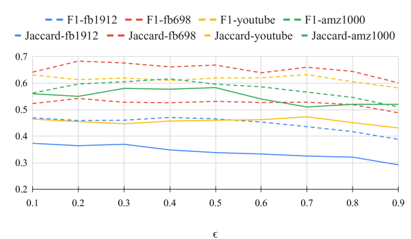
(a) Effect of $\epsilon$. Overall a slight decrease in scores can be observed after $\epsilon=0.7$ mark.

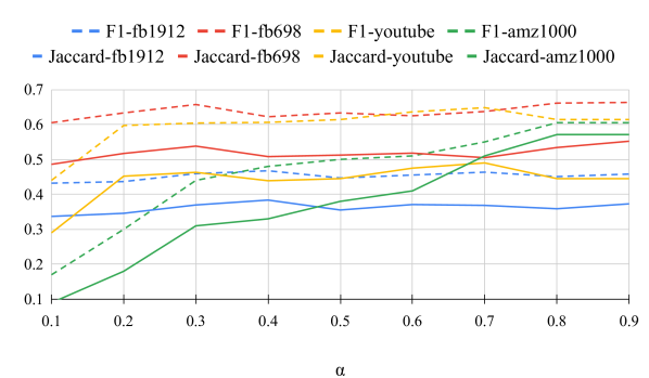
(b) Effect of $\alpha$. The scores generally tend to decrease for small values of $\alpha$.

Figure 1: Effect of hyperparameters on the performance. F1 and Jaccard scores are in solid and dashed lines respectively.

4.6 Training Time

Now we compare the training times of different algorithms in Fig. 2. As some of the baselines are more resource intensive than others, we select aws instance type g4dn.4xlarge for fair comparison of training times. For vGraph, we train for 1000 iterations and for VECoDeR for 1500 iterations. For all other algorithms we use the default parameters as used in section 4.3. We observe that the methods that simply output the node embeddings take relatively less time compared to the algorithms that jointly learn node representations and community assignments e.g VECoDeR , vGraph and CNRL. Among these algorithms VECoDeR is the most time efficient. It consistently trains in less time compared to its direct competitors. For instance, it is about $12$ times faster than ComE for CiteSeer-full and about $40$ times faster compared to vGraph for Cora-full dataset. This provides evidence for lower computational complexity of VECoDeR in Section 3.5.

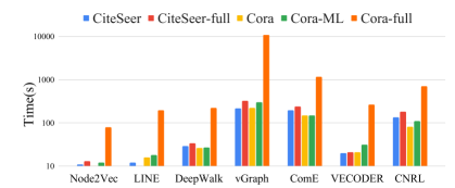
Figure 2: Comparison of running times of different algorithms. We can see that VECoDeR outperforms the direct competitors. The time on y-axis is in log scale.

5 Conclusion

We propose a scalable generative method VECoDeR to simultaneously perform community detection and node representation learning. Our novel approach learns a single community-aware node embedding for both the representation of the node and its context. VECoDeR is scalable due to its low complexity, i.e. ${\mathcal{O}}(|{\mathcal{E}}|K+NKd)$. The experiments on several graph datasets show that VECoDeR consistently outperforms all the competitive baselines on node classification, overlapping community detection and non-overlapping community detection tasks. Moreover, training the VECoDeR is highly time-efficient than its competitors.

Appendix A Derivation of ELBO Bound

$$\text{log}(p_{\theta}({\bm{A}}))=\text{log}\bigg{(}\int\sum\limits_{{\bm{c}}}p_{\theta}({\bm{Z}},{\bm{c}},{\bm{A}})d{\bm{Z}}\bigg{)}$$ (16)

$$=\text{log}\bigg{(}\int\sum\limits_{{\bm{c}}}p({\bm{Z}})\ p_{\theta}({\bm{c}}|{\bm{Z}})\ p_{\theta}({\bm{A}}|{\bm{c}},{\bm{Z}})d{\bm{Z}}\bigg{)}$$ (17)

$$=\text{log}\bigg{(}\mathbb{E}_{({\bm{Z}},{\bm{c}})\sim q_{\phi}({\bm{Z}},{\bm{c}}|{\mathcal{I}})}\bigg{\{}\frac{p({\bm{Z}})\ p_{\theta}({\bm{c}}|{\bm{Z}})\ p_{\theta}({\bm{A}}|{\bm{c}},{\bm{Z}})}{q_{\phi}({\bm{Z}}|{\mathcal{I}})q_{\phi}({\bm{c}}|{\bm{Z}},{\mathcal{I}})}\bigg{\}}\bigg{)}$$ (18)

$$\geq\mathbb{E}_{({\bm{Z}},{\bm{c}})\sim q_{\phi}({\bm{Z}},{\bm{c}}|{\mathcal{I}})}\bigg{\{}\text{log}\bigg{(}\frac{p({\bm{Z}})\ p_{\theta}({\bm{c}}|{\bm{Z}})\ p_{\theta}({\bm{A}}|{\bm{c}},{\bm{Z}})}{q_{\phi}({\bm{Z}}|{\mathcal{I}})q_{\phi}({\bm{c}}|{\bm{Z}},{\mathcal{I}})}\bigg{)}\bigg{\}}$$ (19)

$$=\mathbb{E}_{({\bm{Z}},{\bm{c}})\sim q_{\phi}({\bm{Z}},{\bm{c}}|{\mathcal{I}})}\bigg{\{}\text{log}\bigg{(}\frac{p({\bm{Z}})}{q_{\phi}({\bm{Z}}|{\mathcal{I}})}\bigg{)}$$

$$+\text{log}\bigg{(}\frac{p_{\theta}({\bm{c}}|{\bm{Z}})}{q_{\phi}({\bm{c}}|{\bm{Z}},{\mathcal{I}})}\bigg{)}+\text{log}\bigg{(}p_{\theta}({\bm{A}}|{\bm{c}},{\bm{Z}})\bigg{)}\bigg{\}}$$ (20)

$$=\mathbb{E}_{{\bm{Z}}\sim q_{\phi}({\bm{Z}}|{\mathcal{I}})}\bigg{\{}\text{log}\bigg{(}\frac{p({\bm{Z}})}{q_{\phi}({\bm{Z}}|{\mathcal{I}})}\bigg{)}\bigg{\}}$$

$$+\mathbb{E}_{({\bm{Z}},{\bm{c}})\sim q_{\phi}({\bm{Z}},{\bm{c}}|{\mathcal{I}})}\bigg{\{}\text{log}\bigg{(}\frac{p_{\theta}({\bm{c}}|{\bm{Z}})}{q_{\phi}({\bm{c}}|{\bm{Z}},{\mathcal{I}})}\bigg{)}\bigg{\}}$$

$$+\mathbb{E}_{({\bm{Z}},{\bm{c}})\sim q_{\phi}({\bm{Z}},{\bm{c}}|{\mathcal{I}})}\bigg{\{}\text{log}\bigg{(}p_{\theta}({\bm{A}}|{\bm{c}},{\bm{Z}})\bigg{)}\bigg{\}}.$$ (21)

Where (19) follows from Jensen’s Inequality. First term of (21) is given by:

$$\mathbb{E}_{{\bm{Z}}\sim q_{\phi}({\bm{Z}}|{\mathcal{I}})}\bigg{\{}\text{log}\bigg{(}\frac{p({\bm{Z}})}{q_{\phi}({\bm{Z}}|{\mathcal{I}})}\bigg{)}\bigg{\}}$$

$$=\sum\limits_{i=1}^{N}\mathbb{E}_{{\bm{z}}_{i}\sim q_{\phi}({\bm{z}}_{i}|{\mathcal{I}})}\bigg{\{}\text{log}\bigg{(}\frac{p({\bm{z}}_{i})}{q_{\phi}({\bm{z}}_{i}|{\mathcal{I}})}\bigg{)}\bigg{\}}$$ (22)

$$=-\sum\limits_{i=1}^{N}D_{KL}(q_{\phi}({\bm{z}}_{i}|{\mathcal{I}})\ ||\ p({\bm{z}}_{i})).$$ (23)

Second term of Eq. (21) can be derived as:

$$\mathbb{E}_{({\bm{Z}},{\bm{c}})\sim q_{\phi}({\bm{Z}},{\bm{c}}|{\mathcal{I}})}\bigg{\{}\text{log}\bigg{(}\frac{p_{\theta}({\bm{c}}|{\bm{Z}})}{q_{\phi}({\bm{c}}|{\bm{Z}},{\mathcal{I}})}\bigg{)}\bigg{\}}$$

$$=\sum\limits_{i=1}^{N}\mathbb{E}_{({\bm{z}}_{i},c_{i})\sim q_{\phi}({\bm{z}}_{i},c_{i}|{\mathcal{I}})}\bigg{\{}\text{log}\bigg{(}\frac{p_{\theta}(c_{i}|{\bm{z}}_{i})}{q_{\phi}(c_{i}|{\bm{z}}_{i},{\mathcal{I}})}\bigg{)}\bigg{\}}$$ (24)

$$\approx\sum\limits_{i=1}^{N}\frac{1}{M}\sum\limits_{m=1}^{M}\mathbb{E}_{c_{i}\sim q_{\phi}(c_{i}|{\bm{z}}_{i}^{(m)},{\mathcal{I}})}\bigg{\{}\text{log}\bigg{(}\frac{p_{\theta}(c_{i}|{\bm{z}}_{i}^{(m)})}{q_{\phi}(c_{i}|{\bm{z}}_{i}^{(m)},{\mathcal{I}})}\bigg{)}\bigg{\}}$$ (25)

$$=-\sum\limits_{i=1}^{N}\frac{1}{M}\sum\limits_{m=1}^{M}D_{KL}(q_{\phi}(c_{i}|{\bm{z}}_{i}^{(m)},{\mathcal{I}})\ ||\ p_{\theta}(c_{i}|{\bm{z}}_{i}^{(m)}))$$ (26)

where (25) follows from Eq. (24) by replacing the expectation over ${\bm{z}}_{i}$ with sample mean by generating $M$ samples ${\bm{z}}_{i}^{(m)}$ from distribution $q({\bm{z}}_{i}|{\mathcal{I}})$. Assuming $a_{ij}\in[0,1]\ \forall i$, the third term of Eq. (21) is the negative of binary cross entropy (BCE) between observed and predicted edges.

$$\mathbb{E}_{({\bm{Z}},{\bm{c}})\sim q_{\phi}({\bm{Z}},{\bm{c}}|{\mathcal{I}})}\bigg{\{}\text{log}\bigg{(}p_{\theta}({\bm{A}}|{\bm{c}},{\bm{Z}})\bigg{)}\bigg{\}}$$

$$\quad=\sum\limits_{(i,j)\in{\mathcal{E}}}\mathbb{E}_{({\bm{z}}_{i},{\bm{z}}_{j},c_{i},c_{j})\sim q_{\phi}({\bm{z}}_{i},{\bm{z}}_{j},c_{i},c_{j}|{\mathcal{I}})}\bigg{\{}$$

$$\quad\quad\quad\quad\quad\quad\text{log}\bigg{(}p_{\theta}(a_{ij}|c_{i},c_{j},{\bm{z}}_{i},{\bm{z}}_{j})\bigg{)}\bigg{\}}$$ (27)

Hence, by substituting Eq. (23) and Eq. (26) in Eq. (21), we get the ELBO bound as:

$$\mathcal{L}_{ELBO} \approx$$

$$- \sum\limits_{i=1}^{N}D_{KL}(q_{\phi}({\bm{z}}_{i}|{\mathcal{I}})\ ||\ p({\bm{z}}_{i}))$$

$$- \sum\limits_{i=1}^{N}\frac{1}{M}\sum\limits_{m=1}^{M}D_{KL}(q_{\phi}(c_{i}|{\bm{z}}_{i}^{(m)},{\mathcal{I}})\ ||\ p_{\theta}(c_{i}|{\bm{z}}_{i}^{(m)}))$$

$$+ \sum\limits_{(i,j)\in{\mathcal{E}}}\mathbb{E}_{({\bm{z}}_{i},{\bm{z}}_{j},c_{i},c_{j})\sim q_{\phi}({\bm{z}}_{i},{\bm{z}}_{j},c_{i},c_{j}|{\mathcal{I}})}\bigg{\{}$$

$$\quad\quad\quad\quad\text{log}\bigg{(}p_{\theta}(a_{ij}|c_{i},c_{j},{\bm{z}}_{i},{\bm{z}}_{j})\bigg{)}\bigg{\}}$$ (28)

Appendix B Visualization

Our experiments demonstrate that a single community-aware node embedding is sufficient to aid in both the node representation and community assignment tasks. This is also qualitatively demonstrated by graph visualizations of node embeddings (obtained via t-SNE [Maaten and Hinton, 2008]) and inferred communities for two datasets, fb107 and fb3437, presented in Fig. 3.

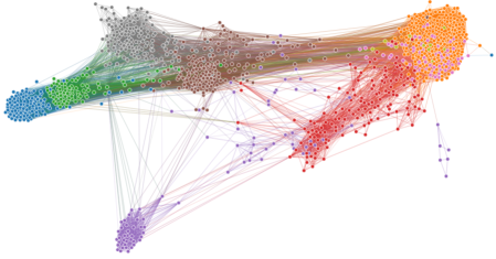
(a) fb107

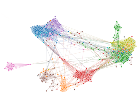
(b) fb3437

Figure 3: Graph visualization with community assignments (better viewed in color)

References

- Ahn et al. [2010] Yong-Yeol Ahn, James P Bagrow, and Sune Lehmann. Link communities reveal multiscale complexity in networks. nature, 466(7307):761–764, 2010.
- Bojchevski and Günnemann [2017] Aleksandar Bojchevski and Stephan Günnemann. Deep gaussian embedding of graphs: Unsupervised inductive learning via ranking. arXiv preprint arXiv:1707.03815, 2017.
- Cao et al. [2015] Shaosheng Cao, Wei Lu, and Qiongkai Xu. Grarep: Learning graph representations with global structural information. In Proceedings of the 24th ACM International on Conference on Information and Knowledge Management, CIKM ’15, page 891–900, New York, NY, USA, 2015. Association for Computing Machinery.
- Cavallari et al. [2017] Sandro Cavallari, Vincent W Zheng, Hongyun Cai, Kevin Chen-Chuan Chang, and Erik Cambria. Learning community embedding with community detection and node embedding on graphs. In Proceedings of the 2017 ACM on Conference on Information and Knowledge Management, pages 377–386, 2017.
- Derényi et al. [2005] Imre Derényi, Gergely Palla, and Tamás Vicsek. Clique percolation in random networks. Physical review letters, 94(16):160202, 2005.
- Doersch [2016] Carl Doersch. Tutorial on variational autoencoders. arXiv preprint arXiv:1606.05908, 2016.
- Fan et al. [2008] Rong-En Fan, Kai-Wei Chang, Cho-Jui Hsieh, Xiang-Rui Wang, and Chih-Jen Lin. Liblinear: A library for large linear classification. Journal of machine learning research, 9(Aug):1871–1874, 2008.
- Gao et al. [2011] Sheng Gao, Ludovic Denoyer, and Patrick Gallinari. Temporal link prediction by integrating content and structure information. In Proceedings of the 20th ACM international conference on Information and knowledge management, pages 1169–1174, 2011.
- Gilmer et al. [2017] Justin Gilmer, Samuel S Schoenholz, Patrick F Riley, Oriol Vinyals, and George E Dahl. Neural message passing for quantum chemistry. arXiv preprint arXiv:1704.01212, 2017.
- Gopalan and Blei [2013] Prem K Gopalan and David M Blei. Efficient discovery of overlapping communities in massive networks. Proceedings of the National Academy of Sciences, 110(36):14534–14539, 2013.
- Grover and Leskovec [2016] Aditya Grover and Jure Leskovec. node2vec: Scalable feature learning for networks. In Proceedings of the 22nd ACM SIGKDD international conference on Knowledge discovery and data mining, pages 855–864, 2016.
- Hamilton et al. [2017] Will Hamilton, Zhitao Ying, and Jure Leskovec. Inductive representation learning on large graphs. In Advances in neural information processing systems, pages 1024–1034, 2017.
- Jang et al. [2016] Eric Jang, Shixiang Gu, and Ben Poole. Categorical reparameterization with gumbel-softmax. arXiv preprint arXiv:1611.01144, 2016.
- Jia et al. [2019] Yuting Jia, Qinqin Zhang, Weinan Zhang, and Xinbing Wang. Communitygan: Community detection with generative adversarial nets. In The World Wide Web Conference, pages 784–794, 2019.
- Khan et al. [2020] Rayyan Ahmad Khan, Muhammad Umer Anwaar, and Martin Kleinsteuber. Epitomic variational graph autoencoder, 2020.
- Kingma and Ba [2014] Diederik P Kingma and Jimmy Ba. Adam: A method for stochastic optimization. arXiv preprint arXiv:1412.6980, 2014.
- Kipf and Welling [2016a] Thomas N Kipf and Max Welling. Semi-supervised classification with graph convolutional networks. arXiv preprint arXiv:1609.02907, 2016.
- Kipf and Welling [2016b] Thomas N Kipf and Max Welling. Variational graph auto-encoders. arXiv preprint arXiv:1611.07308, 2016.
- Kozdoba and Mannor [2015] Mark Kozdoba and Shie Mannor. Community detection via measure space embedding. In Proceedings of the 28th International Conference on Neural Information Processing Systems - Volume 2, NIPS’15, page 2890–2898, Cambridge, MA, USA, 2015. MIT Press.
- Leskovec and Krevl [2014] Jure Leskovec and Andrej Krevl. SNAP Datasets: Stanford large network dataset collection. http://snap.stanford.edu/data, June 2014.
- Leskovec and Mcauley [2012] Jure Leskovec and Julian J Mcauley. Learning to discover social circles in ego networks. In Advances in neural information processing systems, pages 539–547, 2012.
- Maaten and Hinton [2008] Laurens van der Maaten and Geoffrey Hinton. Visualizing data using t-sne. Journal of machine learning research, 9(Nov):2579–2605, 2008.
- Mikolov et al. [2013] Tomas Mikolov, Kai Chen, Greg Corrado, and Jeffrey Dean. Efficient estimation of word representations in vector space. arXiv preprint arXiv:1301.3781, 2013.
- Perozzi et al. [2014] Bryan Perozzi, Rami Al-Rfou, and Steven Skiena. Deepwalk: Online learning of social representations. In Proceedings of the 20th ACM SIGKDD international conference on Knowledge discovery and data mining, pages 701–710, 2014.
- Ribeiro et al. [2017] Leonardo FR Ribeiro, Pedro HP Saverese, and Daniel R Figueiredo. struc2vec: Learning node representations from structural identity. In Proceedings of the 23rd ACM SIGKDD international conference on knowledge discovery and data mining, pages 385–394, 2017.
- Rozemberczki et al. [2019] Benedek Rozemberczki, Ryan Davies, Rik Sarkar, and Charles Sutton. Gemsec: Graph embedding with self clustering. In Proceedings of the 2019 IEEE/ACM international conference on advances in social networks analysis and mining, pages 65–72, 2019.
- Sun et al. [2019] Fan-Yun Sun, Meng Qu, Jordan Hoffmann, Chin-Wei Huang, and Jian Tang. vgraph: A generative model for joint community detection and node representation learning. In Advances in Neural Information Processing Systems, pages 514–524, 2019.
- Tang and Liu [2011] Lei Tang and Huan Liu. Leveraging social media networks for classification. Data Mining and Knowledge Discovery, 23(3):447–478, 2011.
- Tang et al. [2015] Jian Tang, Meng Qu, Mingzhe Wang, Ming Zhang, Jun Yan, and Qiaozhu Mei. Line: Large-scale information network embedding. In Proceedings of the 24th international conference on world wide web, pages 1067–1077, 2015.
- Tang et al. [2016] Jiliang Tang, Charu Aggarwal, and Huan Liu. Node classification in signed social networks. In Proceedings of the 2016 SIAM international conference on data mining, pages 54–62. SIAM, 2016.
- Tu et al. [2018] Cunchao Tu, Xiangkai Zeng, Hao Wang, Zhengyan Zhang, Zhiyuan Liu, Maosong Sun, Bo Zhang, and Leyu Lin. A unified framework for community detection and network representation learning. IEEE Transactions on Knowledge and Data Engineering, 31(6):1051–1065, 2018.
- Veličković et al. [2017] Petar Veličković, Guillem Cucurull, Arantxa Casanova, Adriana Romero, Pietro Lio, and Yoshua Bengio. Graph attention networks. arXiv preprint arXiv:1710.10903, 2017.
- Velickovic et al. [2019] Petar Velickovic, William Fedus, William L Hamilton, Pietro Liò, Yoshua Bengio, and R Devon Hjelm. Deep graph infomax. 2019.
- Wang et al. [2016] Daixin Wang, Peng Cui, and Wenwu Zhu. Structural deep network embedding. In Proceedings of the 22nd ACM SIGKDD international conference on Knowledge discovery and data mining, pages 1225–1234, 2016.
- Wang et al. [2017] Xiao Wang, Peng Cui, Jing Wang, Jian Pei, Wenwu Zhu, and Shiqiang Yang. Community preserving network embedding. In AAAI, volume 17, pages 203–209, 2017.
- Xie et al. [2013] Jierui Xie, Stephen Kelley, and Boleslaw K Szymanski. Overlapping community detection in networks: The state-of-the-art and comparative study. Acm computing surveys (csur), 45(4):1–35, 2013.
- Yang and Leskovec [2013] Jaewon Yang and Jure Leskovec. Overlapping community detection at scale: a nonnegative matrix factorization approach. In Proceedings of the sixth ACM international conference on Web search and data mining, pages 587–596, 2013.
- Yang and Leskovec [2015] Jaewon Yang and Jure Leskovec. Defining and evaluating network communities based on ground-truth. Knowledge and Information Systems, 42(1):181–213, 2015.
- Yang et al. [2013] Jaewon Yang, Julian McAuley, and Jure Leskovec. Community detection in networks with node attributes. In 2013 IEEE 13th International Conference on Data Mining, pages 1151–1156. IEEE, 2013.
- Yang et al. [2016a] Liang Yang, Xiaochun Cao, Dongxiao He, Chuan Wang, Xiao Wang, and Weixiong Zhang. Modularity based community detection with deep learning. In IJCAI, volume 16, pages 2252–2258, 2016.
- Yang et al. [2016b] Zhilin Yang, William Cohen, and Ruslan Salakhudinov. Revisiting semi-supervised learning with graph embeddings. In International conference on machine learning, pages 40–48. PMLR, 2016.