Diffusion Fails to Make a Stink

Abstract

In this work we consider the question of whether a simple diffusive model can explain the scent tracking behaviors found in nature. For such tracking to occur, both the concentration of a scent and its gradient must be above some threshold. Applying these conditions to the solutions of various diffusion equations, we find that the steady state of a purely diffusive model cannot simultaneously satisfy the tracking conditions when parameters are in the experimentally observed range. This demonstrates the necessity of modelling odor dispersal with full fluid dynamics, where non-linear phenomena such as turbulence play a critical role.

I Introduction

We live in a universe that not only obeys mathematical laws, but on a fundamental level appears determined to keep those laws comprehensible Wigner (1960). The achievements of physics in the three centuries since the publication of Newton’s Principia Mathematica Newton (1999) are largely due to this inexplicable contingency. The predictive power of mathematical methods has spurred its adoption in fields as diverse as social science Weidlich (2006) and history van Vugt (2017). A particular beneficiary in the spread of mathematical modelling has been biology Cohen (2004), which has its origins in Schrödinger’s analysis of living beings as reverse entropy machines Schödinger (1992). Today, mathematical treatments of biological processes abound, modelling everything from epidemic networks Hethcote (2000); Ulrich, Nijhout, and Reed (2006) to biochemical switches Hernansaiz-Ballesteros, Cardelli, and Csikász-Nagy (2018), as well as illuminating deep parallels between the processes driving both molecular biology and silicon computing Dalchau et al. (2018).

One of the most natural applications of mathematical modelling is to understand the sensory faculties through which we experience the world. Newton’s use of a bodkin to deform the back of his eyeball Darrigol (2012); Bryson (2003) was one of many experiments performed to confirm his theory of optics Newton (2012); Nauenberg (2017); Grusche (2015). Indeed, the experience of both sight and sound have been extensively contextualised by the mathematics of optics White et al. (1982); Hunt (2003); Luneburg (1947); Lock (1987) and acoustics Rutherford (1886); Mascarenhas et al. (1998); Gabor (1947); Kruse (1961). In contrast to this, simple models which adequately describe the phenomenological experience of smell are strangely lacking, belying the important role olfaction plays in our perception of the world Sell (2019). A robust model describing scent dispersal is of some importance, as olfaction has the potential to be used in the early diagnosis Bijland, Bomers, and Smulders (2013) of infections Bomers et al. (2012) and cancers Buszewski et al. (2012); Willis et al. (2004); Else (2020). In fact, recent work using canine olfaction to train neural networks in the early detection of prostate cancers Guest et al. (2020) suggests that future technologies will rely on a better understanding of our sense of smell.

In the face of these developments, it seems timely to revisit the mechanism of odorant dispersal, and examine the consequences of modeling it via diffusive processes. Here we explore the consequences of using the mathematics of diffusion to describe the dynamics of odorants. In particular, we wish to understand whether such simple models can account for the capacity of organisms to not only detect odors, but to track them to their origin. In previous work, the process of olfaction inside the nasal cavity has been modeled with diffusion Hahn, Scherer, and Mozell (1994), but the question of whether purely diffusive processes can lead to spatial distributions of scent concentration that enable odor tracking has not been considered.

The phenomenon of diffusion has been known and described for millennia, an early example being Pliny the Elder’s observation that it was the process of diffusion that gave roman cement its strength Pliny (1991); Jackson et al. (2017). Diffusion equations have been applied to scenarios as diverse as predicting a gambler’s casino winnings Gommes and Tharakan (2020) to baking a cake Olszewski (2006). The behavior described by the diffusion equation is the random spread of substances Domb and Offenbacher (1978); Ghosh et al. (2006), with its principal virtue being that it is described by well-understood partial differential equations whose solutions can often be obtained analytically. It is therefore a natural candidate for modelling random-motion transport such as (appropriately in 2020) the spread of viral infections Acioli (2020) or the dispersal of a gaseous substance such as an odorant.

The rest of this paper is organized as follows - in Sec.II, we introduce the diffusion equation, and the conditions required of its solution to both detect and track an odor. Sec.III solves the simplest case of diffusion, which applies in scenarios such as a drop of blood diffusing in water. This model is extended in Sec.IV to include both source and decay terms, which describes e.g. a pollinating flower. Finally Sec.V discusses the results presented in previous sections, which find that the distributions which solve the diffusion equation cannot be reconciled with experiential and empirical realities. Ultimately the processes that enable our sense of smell cannot be captured by a simple phenomenological description of time-independent spatial distributions, and models for the olfactory sense must account for the non-linear Ramshaw (2011) dispersal of odor caused by secondary phenomena such as turbulence.

II Modelling Odor Tracking with Diffusion

We wish to answer the question of whether a simple mathematical model can capture the phenomenon of tracking a scent. We know from experience that it is possible to trace the source of an odorant, so any physical model of the dispersal of odors must capture this fact. The natural candidate model for this is the diffusion equation, which in its most basic (one-dimensional) form is given by Riley and Hobson (2006)

$$\frac{\partial C\left(x,t\right)}{\partial t}-D\frac{\partial^{2}C\left(x,t\right)}{\partial x^{2}}=0$$ (1)

where $C(x,t)$ is the concentration of the diffusing substance, and $D$ is the diffusion constant determined by the microscopic dynamics of the system. For the sake of notational simplicity, all diffusion equations presented in this manuscript will be 1D. An extension to 3D will not change any conclusions that can be drawn from the 1D case, as typically the spatial variables in a diffusion equation are separable, so that a full 3D solution to the equation will simply be the product of the 1D equations (provided the 3D initial condition is the product of 1D conditions).

If an odorant is diffusing according to Eq.(1) or its generalizations, there are two prerequisites for an organism to track the odor to its source. First, the odorant must be detectable, and therefore its concentration at the position of the tracker should exceed a given threshold or Limit Of Detection (LOD) Sell (2006); Nicolas and Romain (2004). Additionally, one must be able to distinguish relative concentrations of the odorant at different positions in order to be able to follow the concentration gradient to its source. Fig. 1 sketches the method by which odors are tracked, with the organism sniffing at different locations (separated by a length $\Delta$) in order to find the concentration gradient that determines which direction to travel in.

We can express these conditions for tracking an odorant with two equations

$$C(x) >C_{T},$$ (2)

$$\frac{C(x)}{C(x+\Delta)} >R$$ (3)

where $C(x)$ is the spatial distribution of odor concentration at some time, $C_{T}$ is the LOD concentration, and $R$ characterises the sensitivity to the concentration gradient when smelling at positions $x$ and $x+\Delta$ (where $x+\Delta$ is further from the scent origin).

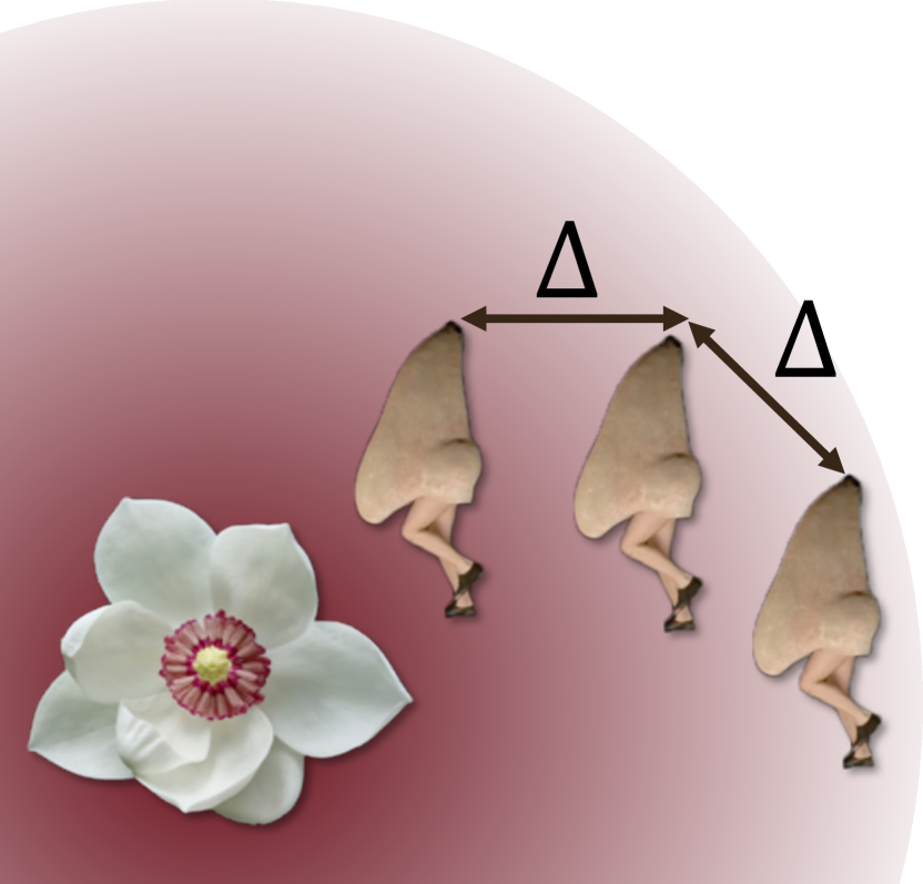
Figure 1: Tracking Odors In order to trace an odor to its source, one sniffs at different locations separated by $\Delta$. If the concentration gradient is sufficiently large, it is possible to determine if one is closer or further from the origin of the smell. Image of the walking nose comes from the Royal Opera House’s production of Shostakovich’s ‘The Nose’.

The biological mechanisms of olfaction determine both $C_{T}$ and $R$, and can be estimated from empirical results. While the LOD varies greatly across the range of odorants and olfactory receptors, the lowest observed thresholds are on the order of 1 part per billion (ppb) Ding et al. (2014). Estimating $R$ is more difficult, but a recent study in mice demonstrated that a 2-fold increase in concentration between inhalations was sufficient to trigger a cellular response in the olfactory bulb Parabucki et al. (2019). Furthermore, comparative studies have demonstrated similar perceptual capabilities between humans and rodents Soh et al. (2013). We therefore assume that in order to track an odor, $R\approx 2$. Values of $\Delta$ will naturally depend on the size of the organism and its frequency of inhalation, but unless otherwise stated we will assume $\Delta=1{\rm m}$.

Having established the basic diffusion model and the criteria necessary for it to reflect reality, we now examine under what conditions the solutions to diffusion equations are able to satisfy Eqs.(2,3).

III The Homeopathic Shark

Popular myth insists that the predatory senses of sharks allow them to detect a drop of its victim’s blood from a mile away, although in reality the volumetric limit of sharks’ olfactory detection is about that of a small swimming pool Meredith and Kajiura (2010). While in general phenomena such as Rayleigh-Taylor instabilities Lyubimova, Vorobev, and Prokopev (2019); Terrones and Carrara (2015); Sun, Zeng, and Tao (2020); Liang et al. (2019) can lead to mixing at the fluid interface, in the current case the similar density of blood and water permits such effects to be neglected. The diffusion of a drop of blood in water is therefore precisely the type of scenario in which Eq.(1) can be expected to apply. To test whether this model can be reconciled to reality, we first calculate the predicted maximum distance $x_{\rm max}$ from which the blood can be detected.

In order to find $C(x,t)$, we stipulate that the mass $M$ of blood is initially described by $C(x,0)=M\delta(x)$. While many methods exist to solve Eq.(1), the most direct is to consider the Fourier transform of the concentration Evans (2010):

$$\tilde{C}(k,t)=\mathcal{F}[C(x,t)]=\int^{\infty}_{-\infty}{\rm d}x\ {\rm e}^{-ikx}C(x,t).$$ (4)

Taking the time derivative and substituting in the diffusion equation we find

$$\frac{\partial\tilde{C}(k,t)}{\partial t}=D\int^{\infty}_{-\infty}{\rm d}x\ {\rm e}^{-ikx}\frac{\partial^{2}C(x,t)}{\partial x^{2}}.$$ (5)

The key to solving this equation is to integrate the right hand side by parts twice. If the boundary conditions are such that both the concentration and its gradient vanish at infinity, then the integration by parts results in

$$\frac{\partial\tilde{C}(k,t)}{\partial t}=-Dk^{2}\tilde{C}(k,t).$$ (6)

This equation has the solution

$$\tilde{C}(k,t)=\tilde{f}(k){\rm e}^{-Dk^{2}t}$$ (7)

where the function $\tilde{f}(k)$ corresponds to the Fourier transform of the initial condition. In this case (where $C(x,0)=M\delta(x)$), $\tilde{f}(k)=M$. The last step is to perform the inverse Fourier transform to recover the solution

$$C(x,t)=\mathcal{F}^{-1}[\tilde{C}(k,t)]=\frac{M}{2\pi}\int^{\infty}_{-\infty}{\rm d}k\ {\rm e}^{-Dk^{2}t+ikx}.$$ (8)

The integral on the right hand side is a Gaussian integral, and can be solved using the standard procedure of completing the square in the integrand exponent Riley and Hobson (2006); Kantorovich (2016a). The final solution to Eq.(1) is then

$$C\left(x,t\right)=\frac{M}{2\pi}{\rm e}^{-\frac{x^{2}}{4Dt}}\int^{\infty}_{-\infty}{\rm d}k\ {\rm e}^{-Dk^{2}t}=\frac{M}{\sqrt{4\pi Dt}}{\rm e}^{-\frac{x^{2}}{4Dt}}.$$ (9)

This expression for the concentration is dependent on both time and space, however for our purposes we wish to understand the threshold sensitivity with respect to distance. To that end, we consider the concentration $C^{*}\left(x\right)$, which describes the highest concentration at each point in space across all of time. This is derived by calculating the time which maximises $C(x,t)$ at each point in $x$:

$$\frac{\partial C\left(x,t\right)}{\partial t} =\frac{M}{\sqrt{4\pi Dt}}{\rm e}^{-\frac{x^{2}}{4Dt}}\left(\frac{x^{2}}{4Dt^{2}}-\frac{1}{2t}\right),$$ (10)

$$\frac{\partial C\left(x,t^{*}\right)}{\partial t} =0\implies t^{*}=\frac{x^{2}}{2D}.$$ (11)

Using this, we have

$$C^{*}\left(x\right)=C\left(x,t^{*}\right)=\frac{M}{\sqrt{2\pi e}x},$$ (12)

where $e$ is Euler’s number. This distribution represents a “best-case” scenario, where one happens to be in place at the right time for the concentration to be at its maximum. Interestingly, while the time of maximum concentration depends on $D$, the concentration itself is entirely insensitive to the microscopic dynamics governing $D$ - the maximum distance a transient scent can be detected is the same whether the shark is swimming through water or treacle!

The threshold detection distance $x_{\rm max}$ can be estimated from Eq.(2) using $x_{\rm max}=\frac{M}{\sqrt{2\pi e}C_{T}}$. For a mass of blood $M=1\rm{g}$ and an estimated LOD of $C_{T}=1\rm{ppb}\sim 1\mu\rm{gm^{-3}}$. As we are working in one dimension we take the cubic root of this threshold to obtain $x_{\rm{max}}\approx 25\rm{m}$. While this seems a believable threshold for detection distances, is it possible to track the source of the odor from this distance? Returning to Eq.(10), the ratio when the concentration is maximal at $x$ is

$$\frac{C(x,t^{*})}{C(x+\Delta,t^{*})}=\exp\left(\frac{\Delta}{x}+\frac{\Delta^{2}}{2x^{2}}\right).$$ (13)

Note that this expression assumes that the timescale over which the concentration changes is much slower than the time between inhalations, hence we compare the concentrations at $x$ and $x+\Delta$ at the same time $t^{*}$. Setting $\frac{C(x_{\max},t^{*})}{C(x_{\max}+\Delta,t^{*})}=R$, we obtain

$$x_{\rm max}=\frac{\Delta\left(1+\sqrt{1+2\ln\left(R\right)}\right)}{2\ln\left(R\right)}.$$ (14)

For the sensitivity $R=2$, $x_{\rm max}\approx 1.8\Delta$. This means that in order to track the scent, the shark has to start on the order of $\Delta$ away from it. Fig.2 shows that to obtain a gradient sensitivity at comparable distances to the LOD distance for $\Delta=1$m would require $R\approx 1.04$. Even in this idealised scenario, the possibility of the shark being able to distinguish and act on a 4% increase in concentration is remote. This suggests that the diffusion model is doing a poor job capturing the real physics of the blood dispersion, and/or the shark’s ability to sense a gradient is somehow improved when odorants are at homeopathically low concentrations. Here we see the first example of a theme which will recur in later sections - diffusive processes generate odorant gradients which are too shallow to follow when one is close to $x_{\rm max}$.

An important caveat should be made to this and later results, namely that the odor tracking strategy we have considered depends purely on the spatial concentration distribution at a particular moment in time. In reality, sharks are just one of a variety of species which rely on scent arrival time to process and perceive odors Gardiner and Atema (2010); Dalal, Gupta, and Haddad (2020). One might reasonably ask whether this additional capacity could assist in the detection of purely diffusing odors, using a tracking strategy that incorporates memory effects. For the moment, it suffices to note that the timescales in which diffusion operates will be far slower than any time-dependent tracking mechanism. We shall find in Sec. IV however that the addition of advective processes to diffusion will force us to revisit this assumption.

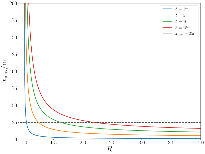
Figure 2: Gradient Sensitivity: The maximum trackable distance depends strongly on both the minimum gradient sensitivity $R$ and the spacing between inhalation $\Delta$. In order to obtain an $x_{\rm max}$ comparable with that associated with the LOD using $R=2$, $\Delta$ must be on the order of $x_{\rm max}$.

IV Adding a source

The simple diffusion model in the previous section predicted that at any scent found at the limit of detection would have a concentration gradient too small to realistically track. This is clearly at odds with lived experience, so we now consider a more realistic system, where there is a continuous source of odorant molecules (e.g. a pollinating flower). In this case our diffusion equation is

$$\frac{\partial C\left(x,t\right)}{\partial t}-D\frac{\partial^{2}C\left(x,t\right)}{\partial x^{2}}+KC(x,t)=f\left(x,t\right)$$ (15)

where $f\left(x,t\right)$ is a source term describing the product of odorants, and $K$ is a decay constant modelling the finite lifetime of odorant molecules.

Finding a solution to this equation is more nuanced than the previous example, due to the inhomogeneous term $f(x,t)$. For now, let us ignore this term, and consider only the effect of the $KC(x,t)$ decay term. In this case, the same Fourier transform technique can be repeated (using the initial condition $C(x,0)=C_{0}\delta(x)$), leading to the solution $C_{K}(x,t)$:

$$C_{K}(x,t)=\frac{C_{0}}{\sqrt{4\pi Dt}}{\rm e}^{-\frac{x^{2}}{4Dt}-Kt}.$$ (16)

This is almost identical to our previous solution, differing only in the addition of a decay term $Kt$ to the exponent.

Incorporating the source term $f(x,t)$ presents more of a challenge, but it can be overcome with the use of a Green’s function Rother (2017). First we postulate that the solution to the diffusion equation can be expressed as

$$C\left(x,t\right)=\int_{0}^{\infty}{\rm d}\tau\int_{-\infty}^{\infty}{\rm d}\xi\ G\left(x,\xi,t,\tau\right)f\left(\xi,\tau\right),$$ (17)

where $G$ is known as the Green’s function. Note that for a solution of this form to exist, the right hand side must satisfy the same properties as $C$, namely that the integral of $G\left(x,\xi,t,\tau\right)f\left(\xi,\tau\right)$ under $\tau$ and $\xi$ is an integrable, normalisable function. In order for Eq.(17) to satisfy Eq.(15), $G$ must itself satisfy:

$$\frac{\partial G\left(x,\xi,t,\tau\right)}{\partial t}- D\frac{\partial^{2}G\left(x,\xi,t,\tau\right)}{\partial x^{2}}$$

$$+ KG\left(x,\xi,t,\tau\right)=\delta(t-\tau)\delta(x-\xi)$$ (18)

Note that the consistency of Eq.(17) with Eq.(15) can be easily verified by substituting Eq.(18) into it.

At first blush, this Green’s function equation looks no easier to solve than the original diffusion equation for $C(x,t)$. Crucially however, the inhomogeneous forcing term $f(x,t)$ has been replaced by a product of delta functions which may be analytically Fourier transformed. Performing this transformation on $x$, we find

$$\frac{\partial\tilde{G}\left(k,\xi,t,\tau\right)}{\partial t}-(Dk^{2}-K)\tilde{G}\left(k,\xi,t,\tau\right)={\rm e}^{-ik\xi}\delta(t-\tau).$$ (19)

We can bring the entirety of the left hand side of this expression under the derivative with the use of an integrating factor Kantorovich (2016b). In this case, we observe that

$$\frac{\partial}{\partial t}\left({\rm e}^{-(Dk^{2}-K)t}\tilde{G}\left(k,\xi,t,\tau\right)\right) ={\rm e}^{-(Dk^{2}-K)t}\bigg{[}\frac{\partial\tilde{G}\left(k,\xi,t,\tau\right)}{\partial t}$$

$$-(Dk^{2}-K)\tilde{G}\left(k,\xi,t,\tau\right)\bigg{]},$$ (20)

which can be substituted into Eq.(19) to obtain

$$\frac{\partial}{\partial t}\left({\rm e}^{-(Dk^{2}-K)t}\tilde{G}\left(k,\xi,t,\tau\right)\right)={\rm e}^{(Dk^{2}-K)t}{\rm e}^{-ik\xi}\delta(t-\tau).$$ (21)

Integrating both sides (together with the initial condition $C(x,0)=G(x,\xi,0,\tau)=0$) yields the Green’s function in $k$ space:

$$\tilde{G}\left(k,\xi,t,\tau\right)=\theta_{H}(t-\tau){\rm e}^{-(Dk^{2}-K)(t-\tau)}{\rm e}^{-ik\xi}$$ (22)

where $\theta_{H}(t-\tau)$ is the Heaviside step function. The inverse Fourier transform of this function is once again a Gaussian integral, and can be solved for in an identical manner to Eq.(8). Performing this integral, we find

$$G(x,\xi,t,\tau)=\theta_{H}(t-\tau)\frac{1}{\sqrt{4\pi D(t-\tau)}}{\rm e}^{-\frac{(x-\xi)^{2}}{4D(t-\tau)}-K(t-\tau)}.$$ (23)

Note that this Green’s function for an inhomogeneous diffusion equation with homogeneous initial conditions is essentially the solution $C_{K}$ given in Eq.(16) to the homogeneous equation with an inhomogeneous initial condition! This surprising result is an example of Duhamel’s principle Tikhonov (1990), which states that the source term can be viewed as the initial condition for a new homogeneous equation starting at each point in time and space. The full solution will then be the integration of each of these homogeneous equations over space and time, exactly as suggested by Eq.(17). From this perspective, it is no surprise that the Green’s function is so intimately connected to the unforced solution.

Equipped with the Green’s function, we are finally ready to tackle Eq.(17). Naturally, this equation is only analytically solvable when $f\left(x,t\right)$ is of a specific form. We shall therefore assume flower’s pollen production is time independent and model it as a point source $f\left(x,t\right)$=$J\delta\left(x\right)$. In this case the concentration is given by

$$C\left(x,t\right)=\frac{J}{\sqrt{4\pi D}}\int_{0}^{t}{\rm d}\tau\ \frac{1}{\sqrt{\tau}}{\rm e}^{-\frac{x^{2}}{4D\tau}-K\tau}.$$ (24)

Now while it is possible to directly integrate this expression, the result is a collection of error functions Riley, Hobson, and Bence (2002). For both practical and aesthetic reasons, we therefore consider the steady state of this distribution $C_{s}(x)$:

$$\lim_{t\to\infty}C\left(x,t\right)=C_{s}(x)=\frac{J}{\sqrt{4\pi D}}\int_{0}^{\infty}{\rm d}\tau\ \frac{1}{\sqrt{\tau}}{\rm e}^{-\frac{x^{2}}{4D\tau}-K\tau}.$$ (25)

This integral initially appears unlike those we have previously encountered, but ultimately we will find that this is yet another Gaussian integral in deep cover. To begin this process, we make the substitution $t=\sqrt{\tau}$:

$$\int_{0}^{\infty}{\rm d}\tau\ \frac{1}{\sqrt{\tau}}{\rm e}^{-\frac{x^{2}}{4D\tau}-K\tau} =2\int_{0}^{\infty}{\rm d}t\ {\rm e}^{-\frac{x^{2}}{4Dt^{2}}-Kt^{2}}$$

$$=\int_{-\infty}^{\infty}{\rm d}t\ {\rm e}^{-\frac{x^{2}}{4Dt^{2}}-Kt^{2}}$$ (26)

where the last equality exploits the even nature of the integrand. At this point we perform another completion of the square, rearranging the exponent to be

$$-\frac{x^{2}}{4Dt^{2}}-Kt^{2}=-\left(\sqrt{K}t-\frac{|x|}{2\sqrt{D}t}\right)^{2}-\sqrt{\frac{K}{D}}|x|.$$ (27)

Combining this with the substitution $t\to\left(\frac{|x|}{2kD}\right)^{\frac{1}{4}}t$, we can express the steady state concentration as:

$$C_{s}(x)=\frac{J{\rm e}^{-\sqrt{\frac{K}{D}}|x|}}{\sqrt{4\pi D}}\left(\frac{|x|}{2KD}\right)^{\frac{1}{4}}\int_{-\infty}^{\infty}{\rm d}t\ {\rm e}^{-\sqrt{\frac{|x|K}{2D}}\left(t-\frac{1}{t}\right)^{2}}.$$ (28)

It may appear that the integral in this expression is no closer to being solved than in Eq.(25), but we can exploit a useful property of definite integrals to finish the job.

Consider a general integral of the form $\int_{-\infty}^{\infty}{\rm d}x\ f(y)$, where $y=x-\frac{1}{x}$. Solving the latter expression, we see that $x$ has two possible branches,

$$x_{\pm}=\frac{1}{2}\left(y\pm\sqrt{y^{2}+4}\right).$$ (29)

Using this, we can split the integral into a term integrating along each branch of $x$:

$$\int_{-\infty}^{\infty}{\rm d}x\ f(y) =\int_{-\infty}^{0_{-}}{\rm d}x_{-}\ f(y)+\int_{0_{+}}^{\infty}{\rm d}x_{+}\ f(y)$$

$$=\int_{-\infty}^{\infty}{\rm d}y\ \left(\frac{{\rm d}x_{-}}{{\rm d}y}+\frac{{\rm d}x_{+}}{{\rm d}y}\right)f(y).$$ (30)

Evaluating the derivatives, we find $\left(\frac{{\rm d}x_{-}}{{\rm d}y}+\frac{{\rm d}x_{+}}{{\rm d}y}\right)=1$, and therefore

$$\int_{-\infty}^{\infty}{\rm d}x\ f(y)=\int_{-\infty}^{\infty}{\rm d}y\ f(y).$$ (31)

This remarkable equality is the Cauchy-Schlömlich transformationCauchy (1823); Amdeberhan et al. (2019), and its generalization to both finite integration limits and a large class of substitutions $y(x)$ is known as Glasser’s master theoremGlasser (1983).

Equipped with Eq.(31), we can immediately recognise Eq.(28) as a Gaussian integral, and evaluate it to obtain our final result

$$C_{S}(x)=\frac{J{\rm e}^{-\lambda\left|x\right|}}{2\sqrt{DK}},$$ (32)

where $\lambda=\sqrt{K/D}$ is the characteristic length scale of the system. Physically, this parameter describes the competition between diffusion and decay. As we shall see, for large $\lambda$ decay dominates the dynamics, quickly forcing odorants down to undetectable concentrations. Conversely for small $\lambda$, diffusion is the principal process, spreading the odorant to the extent that the gradient of the steady state is too shallow to track.

Having finally found our steady state distribution (plotted in Fig.3), we can return to the original question of whether this model admits the possibility of odorant tracking. Substituting $C_{s}(x)$ into Eqs.(2,3), we obtain our maximum distances for surpassing the LOD concentration

$$x_{\rm max}=\lambda^{-1}\ln{\left(\frac{J}{2C_{T}\sqrt{DK}}\right)}$$ (33)

and the gradient sensitivity threshold

$$R_{\rm min}={\rm e}^{\lambda\Delta}.$$ (34)

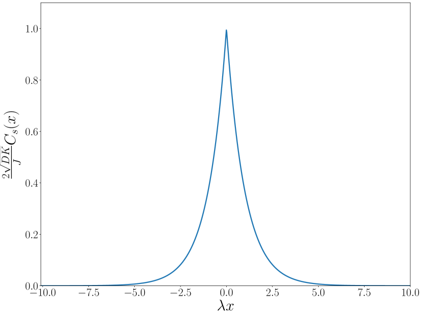
Figure 3: Steady state solution for a diffusing system with both source and decay: While the source term $J$ only determines the maximum concentration at the origin, the degree of exponential fall-off is strongly dependent on $\lambda=\sqrt{\frac{K}{D}}$.

Immediately we see that both of these thresholds are most strongly dependent on the characteristic length scale $\lambda$. For the LOD distance, the presence of a logarithm means that even if the LOD were lowered by an order of magnitude, $C_{T}\to\frac{1}{10}C_{T}$, the change in $x_{\rm max}$ would be only $\approx\frac{2.3}{\lambda}$. This means that for a large detection distance threshold, a small $\lambda$ is imperative.

Conversely, in order for concentration gradients to be detectable, we require $R_{\rm min}\approx 2$. This means that $\lambda\Delta\approx 1$, but as we have shown, a reasonable LOD threshold distance needs $\lambda\ll 1$, making a concentration gradient impossible to detect without an enormous $\Delta$. It’s possible to get a sense of the absurd sensitivities required by this model with the insertion of some specific numbers for a given odorant. Linalool is a potent odorant with an LOD of $C_{T}=3.2\mu{\rm gm^{-3}}$ in air Elsharif, Banerjee, and Buettner (2015). Its half life due to oxidation is $t_{\frac{1}{2}}\approx 1.8\times 10^{7}$s Sköld et al. (2004), from which we obtain $K=\frac{\ln\left(2\right)}{t_{\frac{1}{2}}}\approx 3.8\times 10^{-8}{\rm s}^{-1}$. To find the diffusion constant, we use the Stokes-Einstein relationEinstein (1905) (where $k_{B}$ is the Boltzmann constant and $\eta$ is the fluid’s dynamic viscosityCramer (2012))

$$D=\frac{k_{B}T}{6\pi\eta r},$$ (35)

taking the temperature as $T=288K$ ($15^{\circ}$C, approximately the average surface temperature of Earth). The molar volume of linalool in 178.9 ml${\rm mol^{-1}}$, and if the molecule is modelled as a sphere of radius $r$, we obtain:

$$r=\left(\frac{3}{4\pi N_{A}}\times 178.9\times 10^{-6}\right)^{1/3}{\rm m}=4.13\times 10^{-10}{\rm m},$$ (36)

where $N_{A}\approx 6.02\times 10^{23}$ is Avogadro’s number. At 288K, $\eta\approx 1.8\times 10^{-5}{\rm kgm^{-2}s^{-1}}$ and we obtain $D\approx 2.83\times 10^{-8}{\rm m^{2}s^{-1}}$, which is close to experimentally observed values Filho et al. (2002). Using these figures yields $\lambda=\sqrt{\frac{3.8}{2.8}}{\rm m^{-1}}=1.17{\rm m^{-1}}$, which for $\Delta=1{\rm m}$, gives

$$\frac{C_{s}\left(x\right)}{C_{s}\left(x+\Delta\right)}={\rm e}^{1.17}=3.22$$ (37)

a figure that suggests an easily detectable concentration gradient.

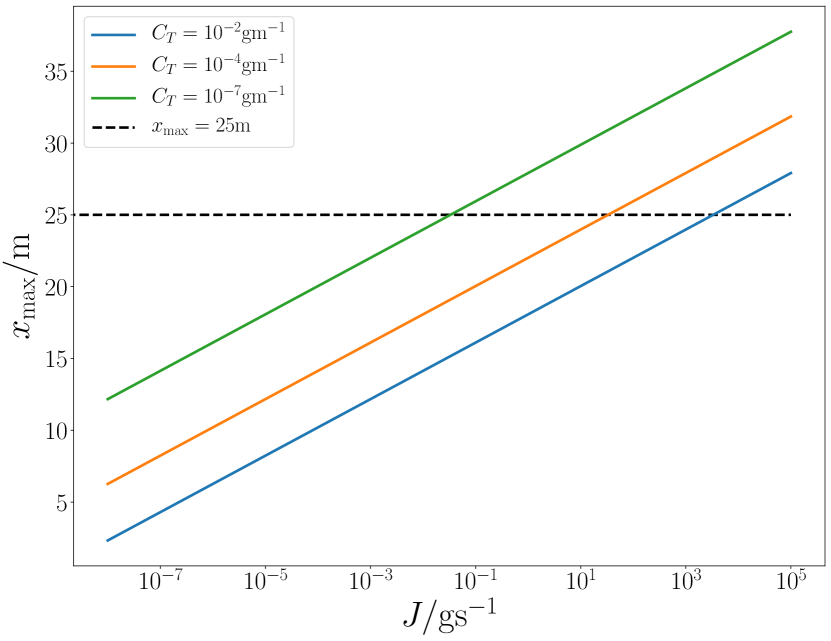
Figure 4: Maximum detection distance as a function of source flux: Using the linalool parameters but varying the LOD threshold, we find that even in the case of $C_{T}=10^{-7}{\rm gm^{-1}}$ (which corresponds to only $\frac{10^{-21}\times N_{A}}{154.24}\sim$ 4 molecules per cubic metre), one requires tens of milligrams of odorant being produced each second for detection at $x_{\rm max}=25$ m. At realistic LOD thresholds, the source flux must increase to kilograms per second to reach the same detection distance.

As noted before however, a large concentration gradient implies that the LOD distance threshold $x_{\rm max}$ must be very small. Substituting the linalool parameters into Eq.(32) with $x_{\rm max}=20{\rm m}$ we find $J=14{\rm gs^{-1}}$, i.e. the flower must be producing a mass of odorant on the order of its own weight. If $x_{\rm max}$ is increased to 25m, then the flower must produce kilograms of matter every second! Fig.4 shows that even with an artificial lowering of the LOD, unphysically large source fluxes are required. Once again, the diffusion model is undermined by the brute fact that completely unrealistic numbers are required for odors to be both detectable and trackable.

Adding Drift

The impossibility of finding physically reasonable parameters which simultaneously satisfy both detection threshold and concentration gradients is due to the exponential nature of the concentration distribution, which requires extremely large parameters to ensure that both Eqs.(2,3) hold. One might question whether the addition of any other dispersal mechanisms can break the steady state’s exponential distribution and perhaps save the diffusive model. A natural extension is to add advection to the diffusion equation, in order to model the effect of wind currents. The effect of this is to add a term $-v(x,t)\frac{\partial C(x,t)}{\partial x}$ to the right hand side of Eq.(15). For a constant drift $v(x,t)\equiv v$, and $v\gg D,K$ the steady state distribution becomes:

$$C_{s}(x)\approx\left\{\begin{array}[]{ll}\frac{J{\rm e}^{-\frac{K}{v}x}}{2v}&x>0,\\ \\ \frac{J{\rm e}^{\frac{v}{D}x}}{2v}&x<0.\end{array}\right.$$ (38)

Another alternative is to consider a stochastic velocity, with a zero mean $\left<v(t)\right>=0$ and Gaussian auto-correlation $\left<v(t)v(t^{\prime})\right>=\sigma\delta(t-t^{\prime})$. In this case the average steady state concentration $\left<C_{s}(x)\right>$ is identical to Eq.(32) with the substitution $D\to D+\sigma$.

In both cases, regardless of whether one adds a constant or stochastic drift the essential problem remains - the steady state distribution remains exponential, and therefore will fail to satisfy one of the two tracking conditions set out in Eqs.(2,3).

There is however a gap through which these diffusion-advection models might be considered a plausible mechanism for odor tracking. By only considering the steady-state, we leave open the possibility that a time-dependent tracking strategy (as mentioned in Sec. III) may be able to follow the scent to its source during the dynamics’ transient period. This will be due precisely to the fact that with the addition of the velocity field $v(x,t)$, the timescale of the odorant dynamics will be greatly reduced. In this case, even if one neglects the heterogeneities that might be induced by a general velocity field, it is possible that the biological processes enabling a time-dependent tracking strategy occupy a timescale compatible with that of the odorant dynamics. In this case, more sophisticated strategies using memory effects could potentially be used to track the diffusion-advection driven odorant distribution.

Flower Fields

We have seen that for a single source of scent production, the steady state of the odor distribution does not support tracking, but what about the scenario where a field (by which we mean an agricultural plot of land, rather than the algebraic structure often used to represent abstract conditions of space) of flowers is generating odorants? We model this by assuming that a set of $2N+1$ flowers are distributed in the region $x\in[-a,a]$ with a spacing $\Delta_{x}\ll a$. In this case the distribution will simply be a linear combination of the distributions for individual flowers:

$$C_{S}(x) =\frac{J}{2\sqrt{DK}}\sum^{N}_{j=-N}{\rm e}^{-\lambda\left|x-j\Delta_{x}\right|}$$

$$=\frac{J}{2\Delta_{x}\sqrt{DK}}\sum^{N}_{j=-N}\Delta_{x}{\rm e}^{-\lambda\left|x-j\Delta_{x}\right|},$$ (39)

where in the second equality we have employed a minor algebraic slight of hand so as to approximate the sum as an integral

$$\sum^{N}_{j=-N}\Delta_{x}{\rm e}^{-\lambda\left|x-j\Delta_{x}\right|}\approx\int^{a}_{-a}{\rm d}y\ {\rm e}^{-\lambda\left|x-y\right|}.$$ (40)

Note that this is an approximation of the sum rather than a limit, so as to obtain a final expression for the distribution while avoiding the issue of taking the limit of $\Delta_{x}$ outside the sum. With this approximation, the integral can be evaluated analytically (albeit in a piecewise manner), and the resultant distribution may be seen in Fig.5.

Given that for $|x|<a$ one is already within the region of scent production, we will focus our attention on the region $x>a$ (which by symmetry also describes the region $x<-a$). In this case, we have

$$C_{S}(x>a)\approx\frac{J{\rm e}^{-\lambda x}}{2\Delta_{x}\sqrt{DK}}\int^{a}_{-a}{\rm d}y\ {\rm e}^{\lambda y}=\frac{J\sinh(\lambda a){\rm e}^{-\lambda x}}{\lambda\Delta_{x}\sqrt{DK}}.$$ (41)

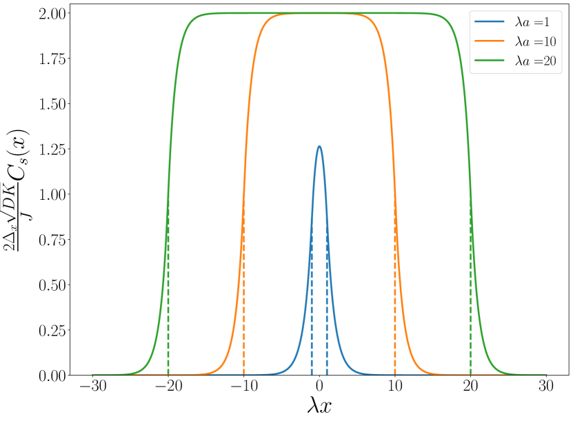
Figure 5: Concentrations for a field of of flowers: The distribution for a field of flowers will rapidly saturate inside the source region $x\in[-a,a]$ (indicated by dashed lines), but outside this region the concentration distribution remains exponential.

This distribution is identical to Eq.(32) with the substitution $J\to J\frac{2\sinh(\lambda a)}{\lambda\Delta_{x}}$. One’s initial impression might be that this would reduce the necessary value of $J$ for a given LOD threshold by many orders of magnitude, but we must also account for the shift in the scent origin away from $x=0$ to $x=a$. This means that the proper comparison to (for example) $x_{\rm max}=20$m in the single flower case would be to take $x_{\rm max}=(20+a)$m here. This extra factor of $a$ will approximately cancel the scaling of $J$ by $2\sinh(\lambda a)$ (for $a>1$). It therefore follows that the effective scaling of $J$ in this region compared to the single flower is only $J\to\frac{J}{\lambda\Delta_{x}}$. Inserting this into Eq.(33), one sees that for a given $J$, the LOD distance is improved only logarithmically by an additional $\lambda^{-1}\ln(\frac{1}{\lambda\Delta_{x}})$. Depending on $\Delta_{x}$, this may improve $x_{\rm max}$ somewhat, but would require extraordinarily dense flower fields to be consistent with the detection distances found in nature. We again stress that these results consider only the steady state distribution, and are therefore subject to the same caveats discussed previously.

V Discussion

My Dog has no nose. How does he smell? Terrible.

In this paper we have considered the implications for olfactory tracking when odorant dispersal is modelled as a purely diffusive process. We find that even under quite general conditions, the steady state distribution of odorants is exponential in its nature. This exponent is characterized by a length scale $\lambda$ whose functional form depends on whether the mechanisms of drift and decay are present. The principal result presented here is that in order to track an odor, it is necessary for odor concentrations both to exceed the LOD threshold, and have a sufficiently large gradient to allow the odor to be tracked to its origin. Analysis showed that in exponential models these two requirements are fundamentally incompatible, as large threshold detection distances require small $\lambda$, while detectable concentration gradients need large $\lambda$. Estimates of the size of other parameters necessary to compensate for having an unsuitable $\lambda$ in one of the tracking conditions lead to entirely unphysical figures either in concentration thresholds or source fluxes of odorant molecules. We emphasise however that these conclusions are drawn on the basis of an odor tracking strategy that incorporates only the spatial information of the odorant distribution, an assumption that holds only when the timescales of the odorant dynamics and scent perception are sufficiently separated.

In reality, it is well known that odorants disperse in long, turbulent plumes Murlis, Willis, and Cardé (2000); Moore and Crimaldi (2004) which exhibit extreme fluctuations in concentration on short length scales Mylne and Mason (1991). It is these spatio-temporal patterns that provide sufficient stimulation to the olfactory senses Vickers et al. (2001). The underlying dynamics that generate these plumes are a combination of the microscopic diffusive dynamics discussed here, and the turbulent fluid dynamics of the atmosphere, which depend on both the scale and dimensionality of the modeled system Weissburg et al. (2002). This gives rise to a velocity field $v(x,t)$ that has a highly non-linear spatiotemporal dependence Lukaszewicz (2016), a property that is inherited by the concentration distribution it produces. For a schematic example of how turbulence can affect concentration distributions, see Figs.1-5 of Ref.[72] Richardson and Walker (1926). These macroscopic processes are far less well understood than diffusion due to their non-linear nature, but we have shown here that odor tracking strategies on the length scales observed in nature Lytridis et al. (2001) are implausible for a purely diffusive model.

Although a full description of turbulent behaviour is beyond a purely diffusive model, recurrent attempts have been made to extend these models and approximate the effects of turbulence. These models incorporate time dependent diffusion coefficients Jeon, Chechkin, and Metzler (2014), which leads to anomalous diffusion Klafter, Blumen, and Shlesinger (1987); Cherstvy, Chechkin, and Metzler (2013) and non-homogeneous distributions which may plausibly support odor tracking. In some cases it is even possible to re-express models using convective terms as a set of pure diffusion equations with complex potentials Karedla et al. (2019); Thiele et al. (2020). Such attempts to incorporate (even approximately) the effects of turbulent air flows are important, for as we have seen (through their absence in a purely diffusive model), this phenomenon is the essential process enabling odors to be tracked.

Data Availability

The data that support the findings of this study are available from the corresponding author upon reasonable request.

References

- Wigner (1960) E. P. Wigner, “The unreasonable effectiveness of mathematics in the natural sciences. richard courant lecture in mathematical sciences delivered at new york university, may 11, 1959,” Communications on Pure and Applied Mathematics 13, 1–14 (1960), https://onlinelibrary.wiley.com/doi/pdf/10.1002/cpa.3160130102 .
- Newton (1999) I. Newton, The Principia : mathematical principles of natural philosophy (University of California Press, Berkeley, 1999).
- Weidlich (2006) W. Weidlich, Sociodynamics : a systemic approach to mathematical modelling in the social sciences (Dover, Mineola, N.Y, 2006).
- van Vugt (2017) I. van Vugt, “Using multi-layered networks to disclose books in the republic of letters,” Journal of Historical Network Research 1, 25–51 (2017).
- Cohen (2004) J. E. Cohen, “Mathematics is biology’s next microscope, only better; biology is mathematics’ next physics, only better,” PLoS Biol. 2 (2004), 10.1371/journal.pbio.0020439.
- Schödinger (1992) E. Schödinger, What is life? : the physical aspect of the living cell ; with Mind and matter ; & Autobiographical sketches (Cambridge University Press, Cambridge New York, 1992).
- Hethcote (2000) H. W. Hethcote, “The Mathematics of Infectious Diseases (SIAM REVIEW),” SIAM Rev. 42, 599–653 (2000).
- Ulrich, Nijhout, and Reed (2006) C. M. Ulrich, H. F. Nijhout, and M. C. Reed, “Mathematical modeling: Epidemiology meets systems biology,” Cancer Epidemiol. Biomarkers Prev. 15, 827–829 (2006).
- Hernansaiz-Ballesteros, Cardelli, and Csikász-Nagy (2018) R. D. Hernansaiz-Ballesteros, L. Cardelli, and A. Csikász-Nagy, “Single molecules can operate as primitive biological sensors, switches and oscillators,” BMC Syst. Biol. 12, 1–14 (2018).
- Dalchau et al. (2018) N. Dalchau, G. Szép, R. Hernansaiz-Ballesteros, C. P. Barnes, L. Cardelli, A. Phillips, and A. Csikász-Nagy, “Computing with biological switches and clocks,” Nat. Comput. 17, 761–779 (2018).
- Darrigol (2012) O. Darrigol, A history of optics : from Greek antiquity to the nineteenth century (Oxford University Press, Oxford New York, 2012).
- Bryson (2003) B. Bryson, A short history of nearly everything (Broadway Books, New York, 2003).
- Newton (2012) I. Newton, Opticks (CreateSpace, Lexington, Ky, 2012).
- Nauenberg (2017) M. Nauenberg, “Newton’s theory of the atmospheric refraction of light,” American Journal of Physics 85, 921–925 (2017), https://doi.org/10.1119/1.5009672 .
- Grusche (2015) S. Grusche, “Revealing the nature of the final image in newton’s experimentum crucis,” American Journal of Physics 83, 583–589 (2015), https://doi.org/10.1119/1.4918598 .
- White et al. (1982) H. W. White, P. E. Chumbley, R. L. Berney, and V. H. Barredo, “Undergraduate laboratory experiment to measure the threshold of vision,” American Journal of Physics 50, 448–450 (1982), https://doi.org/10.1119/1.12831 .
- Hunt (2003) J. L. Hunt, “The roget illusion, the anorthoscope and the persistence of vision,” American Journal of Physics 71, 774–777 (2003), https://doi.org/10.1119/1.1575766 .
- Luneburg (1947) R. K. Luneburg, Math. Anal. Binocul. vision. (Princeton University Press, Princeton, NJ, US, 1947) pp. vi, 104–vi, 104.
- Lock (1987) J. A. Lock, “Fresnel diffraction effects in misfocused vision,” American Journal of Physics 55, 265–269 (1987), https://doi.org/10.1119/1.15175 .
- Rutherford (1886) W. Rutherford, “A New Theory Of Hearing,” J. Anat Physiol. 21, 166–168 (1886).
- Mascarenhas et al. (1998) F. M. F. Mascarenhas, C. M. Spillmann, J. F. Lindner, and D. T. Jacobs, “Hearing the shape of a rod by the sound of its collision,” American Journal of Physics 66, 692–697 (1998), https://doi.org/10.1119/1.18934 .
- Gabor (1947) D. Gabor, “Acoustical Quanta And The Theory of Hearing,” Nature 159, 591 (1947).
- Kruse (1961) O. E. Kruse, “Hearing and seeing beats,” American Journal of Physics 29, 645–645 (1961), https://doi.org/10.1119/1.1937877 .
- Sell (2019) C. Sell, Fundamentals of fragrance chemistry (Wiley-VCH, Weinheim, Germany, 2019).
- Bijland, Bomers, and Smulders (2013) L. R. Bijland, M. K. Bomers, and Y. M. Smulders, “Smelling the diagnosis A review on the use of scent in diagnosing disease,” Neth. J. Med. 71, 300–307 (2013).
- Bomers et al. (2012) M. K. Bomers, M. A. Van Agtmael, H. Luik, M. C. Van Veen, C. M. Vandenbroucke-Grauls, and Y. M. Smulders, “Using a dog’s superior olfactory sensitivity to identify Clostridium difficile in stools and patients: Proof of principle study,” BMJ 345, 1–8 (2012).
- Buszewski et al. (2012) B. Buszewski, T. Ligor, T. Jezierski, A. Wenda-Piesik, M. Walczak, and J. Rudnicka, “Identification of volatile lung cancer markers by gas chromatography-mass spectrometry: Comparison with discrimination by canines,” Anal. Bioanal. Chem. 404, 141–146 (2012).
- Willis et al. (2004) C. M. Willis, S. M. Church, C. M. Guest, W. A. Cook, N. McCarthy, A. J. Bransbury, M. R. T. Church, and J. C. T. Church, “Olfactory detection of human bladder cancer by dogs: proof of principle study,” BMJ 329, 712 (2004), https://www.bmj.com/content/329/7468/712.full.pdf .
- Else (2020) H. Else, “Can dogs smell COVID? here’s what the science says,” Nature 587, 530–531 (2020).
- Guest et al. (2020) C. Guest, R. Harris, K. S. Sfanos, E. Shrestha, A. W. Partin, B. Trock, L. Mangold, R. Bader, A. Kozak, S. Mclean, J. Simons, H. Soule, T. Johnson, W.-Y. Lee, Q. Gao, S. Aziz, P. Stathatou, S. Thaler, S. Foster, and A. Mershin, “Feasibility of integrating canine olfaction with chemical and microbial profiling of urine to detect lethal prostate cancer,” bioRxiv (2020), 10.1101/2020.09.09.288258, https://www.biorxiv.org/content/early/2020/09/10/2020.09.09.288258.full.pdf .
- Hahn, Scherer, and Mozell (1994) I. Hahn, P. W. Scherer, and M. M. Mozell, “A mass transport model of olfaction,” J. Theor. Biol. 167, 115–128 (1994).
- Pliny (1991) Pliny, Natural history, a selection (Penguin Books, London, England New York, NY, USA, 1991).
- Jackson et al. (2017) M. D. Jackson, S. R. Mulcahy, H. Chen, Y. Li, Q. Li, P. Cappelletti, and H.-R. Wenk, “Phillipsite and Al-tobermorite mineral cements produced through low-temperature water-rock reactions in Roman marine concrete,” American Mineralogist 102, 1435–1450 (2017), https://pubs.geoscienceworld.org/ammin/article-pdf/102/7/1435/2638922/am-2017-5993CCBY.pdf .
- Gommes and Tharakan (2020) C. J. Gommes and J. Tharakan, “The péclet number of a casino: Diffusion and convection in a gambling context,” American Journal of Physics 88, 439–447 (2020), https://doi.org/10.1119/10.0000957 .
- Olszewski (2006) E. A. Olszewski, “From baking a cake to solving the diffusion equation,” American Journal of Physics 74, 502–509 (2006), https://doi.org/10.1119/1.2186330 .
- Domb and Offenbacher (1978) C. Domb and E. L. Offenbacher, “Random walks and diffusion,” American Journal of Physics 46, 49–56 (1978), https://doi.org/10.1119/1.11101 .
- Ghosh et al. (2006) K. Ghosh, K. A. Dill, M. M. Inamdar, E. Seitaridou, and R. Phillips, “Teaching the principles of statistical dynamics,” American Journal of Physics 74, 123–133 (2006), https://doi.org/10.1119/1.2142789 .
- Acioli (2020) P. H. Acioli, “Diffusion as a first model of spread of viral infection,” American Journal of Physics 88, 600–604 (2020), https://doi.org/10.1119/10.0001464 .
- Ramshaw (2011) J. D. Ramshaw, “Nonlinear ordinary differential equations in fluid dynamics,” American Journal of Physics 79, 1255–1260 (2011), https://doi.org/10.1119/1.3636635 .
- Riley and Hobson (2006) K. F. Riley and S. Hobson, M.P. Bence, Mathematical methods for physics and engineering (Cambridge University Press, Cambridge, 2006).
- Sell (2006) C. S. Sell, “On the unpredictability of odor,” Angewandte Chemie International Edition 45, 6254–6261 (2006).
- Nicolas and Romain (2004) J. Nicolas and A.-C. Romain, “Establishing the limit of detection and the resolution limits of odorous sources in the environment for an array of metal oxide gas sensors,” Sensors and Actuators B: Chemical 99, 384 – 392 (2004).
- Ding et al. (2014) Z. Ding, S. Peng, W. Xia, H. Zheng, X. Chen, and L. Yin, “Analysis of five earthy-musty odorants in environmental water by HS-SPME/GC-MS,” International Journal of Analytical Chemistry 2014, 1–11 (2014).
- Parabucki et al. (2019) A. Parabucki, A. Bizer, G. Morris, A. E. Munoz, A. D. Bala, M. Smear, and R. Shusterman, “Odor concentration change coding in the olfactory bulb,” eNeuro 6, 1–13 (2019).
- Soh et al. (2013) Z. Soh, M. Saito, Y. Kurita, N. Takiguchi, H. Ohtake, and T. Tsuji, “A Comparison Between the Human Sense of Smell and Neural Activity in the Olfactory Bulb of Rats,” Chemical Senses 39, 91–105 (2013), https://academic.oup.com/chemse/article-pdf/39/2/91/1644534/bjt057.pdf .
- Meredith and Kajiura (2010) T. L. Meredith and S. M. Kajiura, “Olfactory morphology and physiology of elasmobranchs,” J. Exp. Biol. 213, 3449–3456 (2010).
- Lyubimova, Vorobev, and Prokopev (2019) T. Lyubimova, A. Vorobev, and S. Prokopev, “Rayleigh-taylor instability of a miscible interface in a confined domain,” Physics of Fluids 31, 014104 (2019), https://doi.org/10.1063/1.5064547 .
- Terrones and Carrara (2015) G. Terrones and M. D. Carrara, “Rayleigh-taylor instability at spherical interfaces between viscous fluids: Fluid/vacuum interface,” Physics of Fluids 27, 054105 (2015), https://doi.org/10.1063/1.4921648 .
- Sun, Zeng, and Tao (2020) Y. B. Sun, R. H. Zeng, and J. J. Tao, “Elastic rayleigh–taylor and richtmyer–meshkov instabilities in spherical geometry,” Physics of Fluids 32, 124101 (2020), https://doi.org/10.1063/5.0027909 .
- Liang et al. (2019) H. Liang, X. Hu, X. Huang, and J. Xu, “Direct numerical simulations of multi-mode immiscible rayleigh-taylor instability with high reynolds numbers,” Physics of Fluids 31, 112104 (2019), https://doi.org/10.1063/1.5127888 .
- Evans (2010) L. Evans, Partial differential equations (American Mathematical Society, Providence, R.I, 2010).
- Kantorovich (2016a) L. Kantorovich, Mathematics for natural scientists II : advanced methods (Springer, Switzerland, 2016).
- Gardiner and Atema (2010) J. M. Gardiner and J. Atema, “The function of bilateral odor arrival time differences in olfactory orientation of sharks,” Current Biology 20, 1187 – 1191 (2010).
- Dalal, Gupta, and Haddad (2020) T. Dalal, N. Gupta, and R. Haddad, “Bilateral and unilateral odor processing and odor perception,” Communications Biology 3 (2020), 10.1038/s42003-020-0876-6.
- Rother (2017) T. Rother, Green’s functions in classical physics (Springer, Cham, Switzerland, 2017).
- Kantorovich (2016b) L. Kantorovich, Mathematics for natural scientists : fundamentals and basics (Springer, New York, 2016).
- Tikhonov (1990) A. N. Tikhonov, Equations of mathematical physics (Dover Publications, New York, 1990).
- Riley, Hobson, and Bence (2002) K. F. Riley, M. P. Hobson, and S. J. Bence, Mathematical Methods for Physics and Engineering: A Comprehensive Guide, 2nd ed. (Cambridge University Press, 2002).
- Cauchy (1823) A. Cauchy, Ouevre Completes D’Augustin Cauchy (De L’Académie Des Sciences, 1823).
- Amdeberhan et al. (2019) T. Amdeberhan, M. L. Glasser, M. C. Jones, V. Moll, R. Posey, and D. Varela, “The cauchy–schlömilch transformation,” Integral Transforms and Special Functions 30, 940–961 (2019).
- Glasser (1983) M. Glasser, “A remarkable property of definite integrals,” Math Comp 40, 561–563 (1983).
- Elsharif, Banerjee, and Buettner (2015) S. A. Elsharif, A. Banerjee, and A. Buettner, “Structure-odor relationships of linalool, linalyl acetate and their corresponding oxygenated derivatives,” Front. Chem. 3, 1–10 (2015).
- Sköld et al. (2004) M. Sköld, A. Börje, E. Harambasic, and A. T. Karlberg, “Contact allergens formed on air exposure of linalool. Identification and quantification of primary and secondary oxidation products and the effect on skin sensitization,” Chem. Res. Toxicol. 17, 1697–1705 (2004).
- Einstein (1905) A. Einstein, “Über die von der molekularkinetischen theorie der wärme geforderte bewegung von in ruhenden flüssigkeiten suspendierten teilchen,” Annalen der Physik 322, 549–560 (1905).
- Cramer (2012) M. S. Cramer, “Numerical estimates for the bulk viscosity of ideal gases,” Physics of Fluids 24, 066102 (2012), https://doi.org/10.1063/1.4729611 .
- Filho et al. (2002) C. A. Filho, C. M. Silva, M. B. Quadri, and E. A. Macedo, “Infinite dilution diffusion coefficients of linalool and benzene in supercritical carbon dioxide,” Journal of Chemical & Engineering Data 47, 1351–1354 (2002).
- Murlis, Willis, and Cardé (2000) J. Murlis, M. A. Willis, and R. T. Cardé, “Spatial and temporal structures of pheromone plumes in fields and forests,” Physiol. Entomol. 25, 211–222 (2000).
- Moore and Crimaldi (2004) P. Moore and J. Crimaldi, “Odor landscapes and animal behavior: Tracking odor plumes in different physical worlds,” J. Mar. Syst. 49, 55–64 (2004).
- Mylne and Mason (1991) K. R. Mylne and P. J. Mason, “Concentration fluctuation measurements in a dispersing plume at a range of up to 1000 m,” Quarterly Journal of the Royal Meteorological Society 117, 177–206 (1991), https://rmets.onlinelibrary.wiley.com/doi/pdf/10.1002/qj.49711749709 .
- Vickers et al. (2001) N. J. Vickers, T. A. Christensen, T. C. Baker, and J. G. Hildebrand, “Odour-plume dynamics influence the brain’s olfactory code,” Nature 410 (2001).
- Weissburg et al. (2002) M. J. Weissburg, D. B. Dusenbery, H. Ishida, J. Janata, T. Keller, P. J. Roberts, and D. R. Webster, “A multidisciplinary study of spatial and temporal scales containing information in turbulent chemical plume tracking,” Environ. Fluid Mech. 2, 65–94 (2002).
- Lukaszewicz (2016) G. Lukaszewicz, Navier-Stokes equations : an introduction with applications (Springer, Switzerland, 2016).
- Richardson and Walker (1926) L. F. Richardson and G. T. Walker, “Atmospheric diffusion shown on a distance-neighbour graph,” Proceedings of the Royal Society of London. Series A, Containing Papers of a Mathematical and Physical Character 110, 709–737 (1926), https://royalsocietypublishing.org/doi/pdf/10.1098/rspa.1926.0043 .
- Lytridis et al. (2001) C. Lytridis, G. S. Virk, Y. Rebour, and E. E. Kadar, “Odor-based navigational strategies for mobile agents,” Adapt. Behav. 9, 171–187 (2001).
- Jeon, Chechkin, and Metzler (2014) J.-H. Jeon, A. V. Chechkin, and R. Metzler, “Scaled brownian motion: a paradoxical process with a time dependent diffusivity for the description of anomalous diffusion,” Phys. Chem. Chem. Phys. 16, 15811–15817 (2014).
- Klafter, Blumen, and Shlesinger (1987) J. Klafter, A. Blumen, and M. F. Shlesinger, “Stochastic pathway to anomalous diffusion,” Phys. Rev. A 35, 3081–3085 (1987).
- Cherstvy, Chechkin, and Metzler (2013) A. G. Cherstvy, A. V. Chechkin, and R. Metzler, “Anomalous diffusion and ergodicity breaking in heterogeneous diffusion processes,” New Journal of Physics 15, 083039 (2013).
- Karedla et al. (2019) N. Karedla, J. C. Thiele, I. Gregor, and J. Enderlein, “Efficient solver for a special class of convection-diffusion problems,” Physics of Fluids 31, 023606 (2019), https://doi.org/10.1063/1.5079965 .
- Thiele et al. (2020) J. C. Thiele, I. Gregor, N. Karedla, and J. Enderlein, “Efficient modeling of three-dimensional convection–diffusion problems in stationary flows,” Physics of Fluids 32, 112015 (2020), https://doi.org/10.1063/5.0024190 .