Area bound for surfaces in generic gravitational field

Abstract

We define an attractive gravity probe surface (AGPS) as a compact 2-surface $S_{\alpha}$ with positive mean curvature $k$ satisfying $r^{a}D_{a}k/k^{2}\geq\alpha$ (for a constant $\alpha>-1/2$) in the local inverse mean curvature flow, where $r^{a}D_{a}k$ is the derivative of $k$ in the outward unit normal direction. For asymptotically flat spaces, any AGPS is proved to satisfy the areal inequality $A_{\alpha}\leq 4\pi[(3+4\alpha)/(1+2\alpha)]^{2}(Gm)^{2}$, where $A_{\alpha}$ is the area of $S_{\alpha}$ and $m$ is the Arnowitt-Deser-Misner (ADM) mass. Equality is realized when the space is isometric to the $t=$constant hypersurface of the Schwarzschild spacetime and $S_{\alpha}$ is an $r=\mathrm{constant}$ surface with $r^{a}D_{a}k/k^{2}=\alpha$. We adapt the two methods of the inverse mean curvature flow and the conformal flow. Therefore, our result is applicable to the case where $S_{\alpha}$ has multiple components. For anti-de Sitter (AdS) spaces, a similar inequality is derived, but the proof is performed only by using the inverse mean curvature flow. We also discuss the cases with asymptotically locally AdS spaces.

1 Introduction

A strong gravitational field can make any objects trapped in a region. Even photons cannot escape from such a region, which leads to the existence of a black hole. A strong gravitational field would be created by compactly concentrated gravitational sources, and thus the trapped region must be small. The Penrose inequality PI is an argument regarding the area of its boundary; the area of an apparent horizon $A_{\rm AH}$ must satisfy $A_{\rm AH}\leq 4\pi(2Gm)^{2}$, where $m$ is the Arnowitt-Deser-Misner (ADM) mass and $G$ is Newton’s gravitational constant (we use the unit $c=1$). The proof for the Penrose inequality has been carried out for time-symmetric initial data J&W ; H&I ; Bray . To be more precise, those results are applicable for a minimal surface (MS) in an asymptotically flat space with a Ricci scalar that is non-negative everywhere. This version of the inequality is called the Riemannian Penrose inequality.

The Riemannian Penrose inequality may seem to provide a way to test the theory of general relativity. However, if the cosmic censorship holds, an apparent horizon $A_{\rm AH}$ is hidden by an event horizon, inside of which we cannot observe, according to the definition of a black hole. It is desired to derive an inequality that is applicable to a surface outside the event horizon for the purpose of testing general relativity. The authors of this paper have succeeded in deriving such an inequality Shiromizu:2017ego ; we introduced the loosely trapped surface (LTS) as a surface with positive mean curvature $k>0$ satisfying the non-negativity of the derivative of $k$ in the outward unit normal direction $r^{a}D_{a}k\geq 0$, and proved that the LTS satisfies an areal inequality, $A_{\rm LTS}\leq 4\pi(3Gm)^{2}$, where $A_{\rm LTS}$ is the area of the LTS. The upper bound is realized if and only if the space is isometric to the time-constant slice of the Schwarzschild spacetime and the surface is the photon sphere. The photon sphere exists outside the horizon, and thus an LTS is observable for a distant observer. The proof for the areal inequality of the LTS is achieved with the inverse mean curvature flow in Ref. Shiromizu:2017ego .

In this paper, we further generalize the Riemannian Penrose inequality so that it is applicable to a surface in a region where the gravity is moderately strong or even weak. The surface that we consider in this paper is a compact 2-surface $S_{\alpha}$ with positive mean curvature $k$ that satisfies $r^{a}D_{a}k/k^{2}\geq\alpha$ (for a constant $\alpha>-1/2$) in the local inverse mean curvature flow, which we name the attractive gravity probe surface (AGPS). We show that an AGPS with $\alpha$ satisfies $A_{\alpha}\leq 4\pi\left[(3+4\alpha)/(1+2\alpha)\right]^{2}(Gm)^{2}$, where $A_{\alpha}$ is the area of the AGPS. For $\alpha\to\infty$, the AGPS becomes the MS and the Riemannian Penrose inequality is obtained. Moreover, for $\alpha=0$, we have the theorem for the LTS in Ref. Shiromizu:2017ego . Therefore, the inequality for the AGPS is the generalization of the Riemannian Penrose inequality and the areal inequality for the LTS. We derive the inequality in two different ways; one is by using the inverse mean curvature flow Geroch ; J&W ; H&I and the other is by using Bray’s conformal flow Bray . Both methods were applied for proving the Riemannian Penrose inequality. Since Bray’s proof is applicable to a surface with multiple components, our inequality can be applied to an AGPS with multiple components as well.

We also show areal inequalities for AGPSs in asymptotically (locally) anti-de Sitter (AdS) spaces. Since Bray’s proof based on the conformal flow is not applicable to asymptotically (locally) AdS spaces, our inequality is only derived by using the inverse mean curvature flow for these setups.

The rest of this paper is organized as follows. In Sect. 2 we show the proof by usage of the inverse mean curvature flow in the case for asymptotically flat and AdS spaces. We also discuss the case for asymptotically locally AdS spaces. In Sect. 3, we show another proof of the areal inequality for asymptotically flat spaces, by applying Bray’s method Bray . We will give a summary and discussions in Sect. 4. An example of the matching function used in Sect. 3 is presented in Sect. A.

2 Inverse mean curvature flow

One of the ways to prove the Riemannian Penrose inequality is applying the monotonicity of the Geroch energy in the inverse mean curvature flow. The idea of the monotonicity was introduced in order to prove the positivity of the ADM mass by Geroch Geroch . By applying Geroch’s monotonicity, the Riemannian Penrose inequality was proved by Wald and Jang J&W under the assumption of the existence of a global inverse mean curvature flow. This method was extended by Huisken and Ilmanen H&I to resolve the possible singularity formation in the flow. Hence, the monotonicity exists even if a global inverse mean curvature flow cannot be taken. Geroch’s monotonicity was generalized to spaces with negative cosmological constants by Boucher, Horowitz and Gibbons Boucher:1983cv ; Gibbons:1998zr .

We first review the monotonicity with and without the negative cosmological constant, based on Ref. Gibbons:1998zr , in Sect. 2.1. Then, we show the generalized areal inequality in Sect. 2.2. It is applicable also for asymptotically AdS spaces. The areal inequality is further generalized to asymptotically locally AdS spaces, which is shown in Sect. 2.3.

2.1 Geroch Monotonicity

We consider a three-dimensional space $\Sigma$ where the scalar curvature ${}^{(3)}R$ satisfies

$${}^{(3)}R-2\Lambda\geq 0\qquad(\Lambda\leq 0).$$ (1)

Let us introduce an inverse mean curvature flow. We first consider the foliation of $\{S_{y}\}_{y\in{\bf R}}$. The lapse function is denoted by $\varphi$. Geroch’s quasilocal energy of $S_{y}$ is defined as

$$E(y):=\frac{A^{1/2}(y)}{64\pi^{3/2}G}\int_{S_{y}}\left(2{}^{(2)}R-k^{2}-\frac{4\Lambda}{3}\right)dA,$$ (2)

where $A(y)$ is the area, $dA$ is the areal element, and ${}^{(2)}R$ is the scalar curvature of $S_{y}$. Under the condition of the inverse mean curvature flow $k\varphi=1$, the first derivative of $E(y)$ is shown to satisfy the non-negativity

$$\frac{dE(y)}{dy}\ =\ \frac{A^{1/2}(y)}{64\pi^{3/2}}\int_{S_{y}}\Bigl{[}2\varphi^{-2}({\cal D}\varphi)^{2}+\tilde{k}_{ab}\tilde{k}^{ab}+{}^{(3)}R-2\Lambda\Bigr{]}dA\geq 0,$$ (3)

where $\tilde{k}_{ab}$ is the traceless part of the extrinsic curvature $k_{ab}$, i.e.,

$$\tilde{k}_{ab}:=k_{ab}-\frac{1}{2}kg_{ab},$$ (4)

with $g_{ab}$ being the metric of $S_{y}$. Here, we used the assumption that the topology of $S_{y}$ does not change under the flow, and thus, $\int{}^{(2)}RdA$ is a constant for all $S_{y}$ because it is the topological invariant. Therefore, $E(y)$ is an increasing function, which leads to $E(\infty)\geq E(y)$. Since Geroch’s energy at infinity coincides with the ADM mass in an asymptotically flat spacetime and with the Abbott-Deser mass Abbott:1981 or the Ashtekar-Magnon mass Ashtekar:1984 in asymptotically AdS spacetimes, the inequality implies $m\geq E(y)$. If $E(y)$ is expressed with the area of $S_{y}$, we have an areal inequality as shown below.

2.2 Attractive Gravity Probe Surface

In an asymptotically flat space without the cosmological constant, $E(y)$ for a minimal surface (MS) and for a loosely trapped surface (LTS) Shiromizu:2017ego is evaluated as

$$E(y)=\dfrac{1}{2G}\sqrt{\dfrac{A(y)}{4\pi}}\qquad\mbox{and}\qquad E(y)\geq\dfrac{1}{3G}\sqrt{\dfrac{A(y)}{4\pi}},$$ (5)

respectively. Together with the inequality $m\geq E(y)$, they give the inequalities $A(y)\leq 4\pi(2Gm)^{2}$ for an MS and $A(y)\leq 4\pi(3Gm)^{2}$ for an LTS. Let us show similar areal inequalities by considering a broader class of surfaces, which includes MSs and LTSs.

We consider a surface $S_{\alpha}$ satisfying $k>0$ and

$$\frac{r^{a}D_{a}k}{k^{2}}\geq\alpha,$$ (6)

where $\alpha$ is a constant satisfying

$$\alpha>-\frac{1}{2},$$ (7)

and $r^{a}$ is the outward unit normal vector to $S_{\alpha}$, namely $r_{a}=\varphi D_{a}y$. We call a surface satisfying the above conditions an attractive gravity probe surface (AGPS). The limit $\alpha\to\infty$ gives the condition for an MS, i.e. $k=0$, while the case with $\alpha=0$ is corresponding to an LTS Shiromizu:2017ego . Thus, this surface is a generalization of MSs and LTSs. Note that in the limit $\alpha\to-1/2$, $S_{\alpha}$ coincides with the $S^{2}$ surface at spacelike infinity. In this sense, the concept of the AGPS can cover from the surfaces in extremely strong gravity regions to those in very weak gravity regions through choosing the value of $\alpha$ appropriately. We show that its area $A_{\alpha}$ satisfies an inequality similar to the Penrose inequality.

On $S_{\alpha}$, we have a geometrical identity

$$r^{a}D_{a}k\ =\ -\varphi^{-1}{\cal D}^{2}\varphi-\frac{1}{2}{}^{(3)}R+\frac{1}{2}{}^{(2)}R-\frac{1}{2}(k^{2}+k_{ab}k^{ab}).$$ (8)

Integrating this relation over $S_{\alpha}$, we have

$$\frac{1}{2}\int_{S_{\alpha}}{}^{(2)}RdA = \int_{S_{\alpha}}\left[r^{a}D_{a}k+\varphi^{-2}\left(\cal{D}\varphi\right)^{2}+\frac{1}{2}{}^{(3)}R+\frac{1}{2}\tilde{k}_{ab}\tilde{k}^{ab}+\frac{3}{4}k^{2}\right]dA$$ (9)

$$\geq \int_{S_{\alpha}}\left[\left(\frac{3}{4}+\alpha\right)k^{2}+\Lambda\right]dA,$$

where we used the inequalities of Eqs. (1) and (6). Note that in the case without a cosmological constant, $\Lambda=0$, this inequality leads to the positivity of its left-hand side. Thus, as a consequence of the Gauss-Bonnet theorem, the topology of $S_{\alpha}$ is $S^{2}$. Moreover, for a generic negative cosmological constant, $\Lambda\leq 0$, the Gauss-Bonnet theorem gives us

$$\int_{S_{\alpha}}k^{2}dA\leq\left(\frac{3}{4}+\alpha\right)^{-1}\left[2\pi\chi-\Lambda A_{\alpha}\right],$$ (10)

where $A_{\alpha}$ is the area of $S_{\alpha}$ and $\chi$ is the Euler characteristic of $S_{\alpha}$. The Geroch energy $E(y)$ for the surface $S_{\alpha}$ is estimated as

$$\left.E(y)\right|_{S_{\alpha}} = \frac{A_{\alpha}^{1/2}}{64\pi^{3/2}G}\int_{S_{\alpha}}\left(2{}^{(2)}R-k^{2}-\frac{4\Lambda}{3}\right)dA$$ (11)

$$\geq \frac{1+2\alpha}{3+4\alpha}\frac{\chi}{2G}\left(\frac{A_{\alpha}}{4\pi}\right)^{1/2}-\frac{2\alpha}{3(3+4\alpha)}\frac{\Lambda}{G}\left(\frac{A_{\alpha}}{4\pi}\right)^{3/2}.$$

Under the assumption of the global existence of the inverse mean curvature flow, the topology of $S_{\alpha}$ should be $S^{2}$ even in the case with negative cosmological constant, because the flow cannot change the topology of all leaves of the foliation. Then, the inequality $m\geq E(y)$ gives us

$$Gm\geq\frac{1+2\alpha}{3+4\alpha}\left(\frac{A_{\alpha}}{4\pi}\right)^{1/2}-\frac{2\alpha}{3(3+4\alpha)}\Lambda\left(\frac{A_{\alpha}}{4\pi}\right)^{3/2}.$$ (12)

Equality in the inequality of Eq. (12) occurs if and only if equalities hold in the inequalities in Eqs. (3) and (9), i.e., all ${\cal D}_{a}\varphi$, $\tilde{k}_{ab}$ and ${}^{(3)}R-2\Lambda$ vanish on all of $S_{y}$ and $r^{a}D_{a}k/k^{2}=\alpha$ holds on $S_{\alpha}$. Hence, the metric of $\Sigma$ is

$$dl^{2}=\left(1-\frac{2Gm}{r}-\frac{\Lambda}{3}r^{2}\right)^{-1}dr^{2}+r^{2}d\Omega^{2},$$ (13)

which corresponds to the metric of the maximal slice of an AdS-Schwarzschild spacetime (or, for $\Lambda=0$, a Schwarzschild spacetime), and $S_{\alpha}$ is located at $r=\mathrm{constant}$ on which $r^{a}D_{a}k/k^{2}=\alpha$ is satisfied.

Since $\Lambda$ is non-positive, the right-hand side of the inequality of Eq. (12) is an increasing function with respect to $A_{\alpha}$, and the maximum occurs when equality holds. Hence, $A_{\alpha}$ is bounded by the area of the $r=\mathrm{constant}$ surface satisfying $r^{a}D_{a}k/k^{2}=\alpha$ on the maximal slice of the AdS spacetime for $\Lambda<0$, and the Schwarzschild spacetime for $\Lambda=0$.

In asymptotically flat spacetimes without the cosmological constant (i.e. $\Lambda=0$), the inequality of Eq. (12) can be rewritten as

$$A_{\alpha}\leq 4\pi\left(\frac{3+4\alpha}{1+2\alpha}Gm\right)^{2}.$$ (14)

For $\alpha\to\infty$ (the MS) and for $\alpha=0$ (the LTS), the quantity in the bracket of the above inequality becomes

$$\frac{3+4\alpha}{1+2\alpha}Gm=\left\{\begin{array}[]{cc}2Gm&\quad(\alpha\to\infty)\\ 3Gm&\quad(\alpha=0)\end{array}\right..$$ (17)

Hence, the inequality of Eq. (14) includes the known results for the MS and for the LTS.

2.3 Asymptotically Locally AdS Spacetime

One often considers asymptotically locally AdS spacetimes. Simple examples are given by the metric

$$ds^{2}=-f(r)dt^{2}+f^{-1}(r)dr^{2}+r^{2}d\omega_{\kappa}^{2},$$ (18)

with

$$f(r)=\kappa-\frac{2Gm}{r}-\frac{\Lambda}{3}r^{2},$$ (19)

where $\kappa=\pm 1$ or $0$. Here, $d\omega_{\kappa}^{2}$ denotes the metric of a two-dimensional maximally symmetric surface with the Gauss curvature $\kappa$:

$$d\omega_{\kappa}^{2}=\begin{cases}d\theta^{2}+\sin^{2}\theta d\phi^{2}&(\kappa=+1)\\ d\theta^{2}+d\phi^{2}&(\kappa=0)\\ d\theta^{2}+\sinh^{2}\theta d\phi^{2}&(\kappa=-1)\quad.\end{cases}$$ (20)

Note that two-dimensional section of this space can be compactified into a torus in the case of $\kappa=0$, and into a multi-torus in the case of $\kappa=-1$, and such black holes are called topological black holes. See Ref. Aminneborg:1996 for the procedure for making topological black holes.

Based on these vacuum solutions, it is natural to consider asymptotically locally AdS spaces whose metrics asymptote to

$$dl^{2}=f^{-1}(r)dr^{2}+r^{2}d\omega_{\kappa}^{2}$$ (21)

at infinity. Here, the two-dimensional sections with the metric $r^{2}d\omega_{\kappa}^{2}$ are compactified so that it has genus $g=0$ for $\kappa=+1$, $g=1$ for $\kappa=0$ and $g=2,3,\dots$ for $\kappa=-1$. Supposing the existence of a global inverse mean curvature flow, the topology of $S_{\alpha}$ satisfying the inequality of Eq. (6) is the same as that of the compactified two-dimensional sections. We modify the definition of the Geroch energy as

$$E(y):=\frac{A^{1/2}(y)}{(4\omega_{\kappa})^{3/2}G}\int_{S_{y}}\left(2{}^{(2)}R-k^{2}-\frac{4\Lambda}{3}\right)dA,$$ (22)

where $\omega_{\kappa}$ is the area of the compact two-dimensional surface with the metric $d\omega_{\kappa}^{2}$. Then, $E(y)$ converges to $m$ in the limit $y\to\infty$, and we have the inequality

$$Gm\geq\frac{1+2\alpha}{3+4\alpha}\kappa\left(\frac{A_{\alpha}}{\omega_{\kappa}}\right)^{1/2}-\frac{2\alpha}{3(3+4\alpha)}\Lambda\left(\frac{A_{\alpha}}{\omega_{\kappa}}\right)^{3/2},$$ (23)

where we used $\kappa\omega_{\kappa}=2\pi\chi$. Here, the area of the unit compact two-dimensional surface $\omega_{\kappa}$ is given by

$$\omega_{\kappa}=\begin{cases}4\pi&(\kappa=+1)\\ \mbox{arbitrary}&(\kappa=0)\\ 4\pi(g-1)&(\kappa=-1)\quad.\end{cases}$$ (24)

3 Conformal Flow

There is another approach for proving the Riemannian Penrose inequality based on the conformal flow (Bray’s theorem Bray ). It works for the case of a minimal surface with multiple components, and thus it is more generic than the approach based on the inverse mean curvature flow. In this section, with the aid of Bray’s theorem, we prove our inequality of Eq. (14) to make it applicable to an AGPS with multiple components. Since Bray’s approach can only be applied to asymptotically flat spaces (not asymptotically AdS spaces), our areal inequalities for AGPSs are only applicable to asymptotically flat spaces as well.

In Sect. 3.1, we give some definitions required in the theorems and proofs. Our theorem is explicitly shown in Sect. 3.2. Remaining subsections are devoted to the proof. In Sect. 3.3, we show the sketch of the proof. The main idea is as follows. Our initial data $\Sigma$ has boundaries $S^{(i)}$ with $i=1,\dots,n$, each of which is supposed to be one component of an AGPS $S_{\alpha}$. We glue a manifold ${\bar{\Sigma}}^{(i)}$ at each $S^{(i)}$ and we suppose that each ${\bar{\Sigma}}^{(i)}$ has an inner boundary $\mathcal{S}_{0}^{(i)}$ that is a minimal surface. The union of ${\bar{\Sigma}}^{(i)}$ and that of the $S_{0}^{(i)}$ are denoted by $\bar{\Sigma}$ and $\mathcal{S}_{0}$, respectively. $\bar{\Sigma}$ is constructed so that Bray’s method works for $\Sigma\cup\bar{\Sigma}$. There, we see that the proof is completed if the following two statements hold: that the minimal surface ${\cal S}_{0}$ is the outermost surface, and that the extension of the manifold is smooth. The former is proved under certain conditions in Sect. 3.4. With respect to the latter, the extended manifold $\Sigma\cup\bar{\Sigma}$ is generically nonsmooth ($C^{0}$-class) on the gluing surface $S_{\alpha}$. However, we can show the existence of a sequence of smooth manifolds, which uniformly converges to the nonsmooth extended manifold. Therefore, we will be able to apply Bray’s theorem by taking the limit. This issue will be discussed in Sect. 3.5.

3.1 Terminology and Definitions

Let $\Sigma$ be a smooth, asymptotically flat three-manifold with non-negative scalar curvature. Here we recall that $\Sigma$ has boundaries, one of which is infinity and others are denoted by $S$. Everywhere on the boundaries $S$, the mean curvature is supposed to be positive, where the unit normal faces $\Sigma$. (We later define this direction of the normal vector of $S$ as “outward”.)

Note that if $S$ is smooth, the mean curvature flow from $S$ can always be taken at least for a short interval H&I ; HP , and we call it the local mean curvature flow. The explicit definition is shown below.

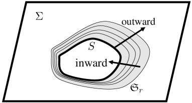
Figure 1: Outward and inward directions of $S$. $S$ (solid curve) is a boundary of $\Sigma$. The outward and inward directions are shown. The local inverse mean curvature flow with foliations ${\mathfrak{S}}_{r}$ (thin curves) is taken in exterior of $S$ (shaded region), if the mean curvature of $S$ with the outward unit normal vector is positive.

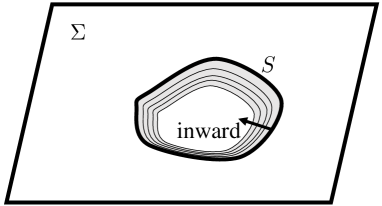
Figure 2: Inward extension from $S$. $S$ (solid curve) is a smooth boundary of $\Sigma$. There may exist a smooth extension of $\Sigma$ from $S$, where the local mean curvature flow (with $r<0$) may be taken. The foliations are shown by thin curves. In Theorem 2, the exsistence of such an extension is assumed. We name the shaded region interior of $S$.

Definition 1.

Local inverse mean curvature flow : Let $\Sigma$ to be a smooth three-dimensional manifold. $S$, which can be multiple, is a two-dimensional smooth compact manifold embeded in $\Sigma$ (or boundary of $\Sigma$) with positive mean curvature. The inverse mean curvature flow is a smooth family of hypersurfaces ${\mathfrak{S}}_{r}:=x(S,r)$, where $x:S\times[0,\varepsilon)\to\Sigma$, satisfying the parabolic evolution equation

$$\left(\frac{\partial x}{\partial r}\right)^{a}=\frac{r^{a}}{k}.$$ (25)

Here, $r^{a}$ is the unit normal to define the mean curvature $k$ assumed to be positive everywhere on ${\mathfrak{S}}_{r}$, and the initial condition is set to be $S=x(S,0)$. Since Eq.(25) is parabolic, a solution exists for a short interval of $r$, $0\leq r<\varepsilon$ H&I ; HP . We call this the “local mean curvature flow” from $S$.

Here we remind the reader that the Penrose inequality is a theorem for the outermost minimal surface. This means that no other minimal surface exists in its exterior region. Similar conditions are required for our theorem, and then we define the term “enclose” as follows. Let $\sigma$ be a compact two-dimensional closed surface (which can be multiple) in a three-dimensional manifold $\Sigma$ with boundary components as well as a single asymptotically flat end. Let ${\cal R}$ be a region which consists of all points $p\in\Sigma\backslash\sigma$ path-connected with the end in $\Sigma\backslash\sigma$. We call ${\cal R}$ the “exterior” region of $\sigma$. We also define the “interior” region of $\sigma$ as $\bar{\cal R}=\Sigma\backslash\left({\cal R}\cup\sigma\right)$. ($\bar{\cal R}$ may be empty.) Then if $\tilde{\cal R}\subset\bar{\cal R}\cup\sigma$, we say that $\sigma$ encloses $\tilde{\cal R}$ (or $\tilde{\cal R}$ is enclosed by $\sigma$).

In the manifold $\Sigma$ that we will consider, the boundary $S$ has positive mean curvature with the unit normal vector $r^{a}$ directing into $\Sigma$, i.e., into the exterior of $S$. The local inverse mean curvature flow is taken in the exterior of $S$. If a direction corresponds to the increase (decrease) in $r$ of Eq. (25), it is called “outward” (“inward”), i.e., $r^{a}$ is the outward normal vector. We sometimes consider an extension of $\Sigma$ from $S$, which is also called the interior of $S$.

The areal inequality will be proved for attractive gravity probe surfaces (AGPSs) introduced in Sect. 2.2. To make our theorem precise, we explicitly give the definition of the AGPS here.

Definition 2.

Attractive gravity probe surfaces (AGPSs) :  Suppose $\Sigma$ to be a smooth three-dimensional manifold with a positive definite metric $g$. A smooth compact surface $S_{\alpha}$ in $\Sigma$ is an attractive gravity probe surface (AGPS) with a parameter $\alpha$ ($\alpha>-1/2$) if the following conditions are satisfied everywhere on $S_{\alpha}$:

(i)

The mean curvature $k$ is positive.

(ii)

With the local mean curvature flow in the neighborhood of $S_{\alpha}$,

$$r^{a}D_{a}k\geq\alpha k^{2}$$ (26)

is satisfied, where $r^{a}$ is the outward unit normal vector to $S_{\alpha}$ used for the definition of $k$, and $D_{a}$ is the covariant derivative with respect to the metric $g$.

3.2 Main Theorem

Now, we present our main theorem:

Theorem 1.

Let $\Sigma$ be an asymptotically flat, three-dimensional, smooth manifold with non-negative Ricci scalar. The boundaries of $\Sigma$ are composed of an asymptotically flat end and an AGPS $S_{\alpha}$, which can have multiple components, with a parameter $\alpha$ in Eq. (26). Here, the unit normal $r^{a}$ used to define the mean curvature is taken to be outward of $S_{\alpha}$. Suppose that there exists a positive number $\varepsilon$ such that, for any leaf ${\mathfrak{S}}_{r}=x(S_{\alpha},r)$ of the foliation in the local mean curvature flow from $S_{\alpha}$, $x:S_{\alpha}\times[0,\varepsilon)\to\Sigma$; no minimal surface satisfying either one of the following conditions exists:

(i)

It encloses (at least) one component of ${\mathfrak{S}}_{r}$.

(ii)

It has boundaries on ${\mathfrak{S}}_{r}$ and its area is less than $4\pi(2Gm)^{2}$.

Then, the area of $S_{\alpha}$ has an upper bound;

$$A_{\alpha}\leq 4\pi\left(\frac{3+4\alpha}{1+2\alpha}Gm\right)^{2},$$ (27)

where $m$ is the ADM mass of the manifold, $G$ is Newton’s gravitational constant. Equality holds if and only if $\Sigma$ is a time-symmetric hypersurface of a Schwarzschild spacetime and $S_{\alpha}$ is a spherically symmetric surface with $r^{a}D_{a}k=\alpha k^{2}$.

In the smooth extension that will be discussed in Sect. 3.5, we will extend $\Sigma$ from $S_{\alpha}$ with a deformation in a neighborhood $U(\subset\Sigma)$ of $S_{\alpha}$, and there, the non-existence conditions $(i)$ and $(ii)$ for minimal surfaces are required for the outer boundary of the deformed region, which is not $S_{\alpha}$ but a leaf of the foliation ${\mathfrak{S}}_{r}$ (see Fig.2). This is because, in Theorem 1, the existence of the smooth extension from $S_{\alpha}$ to the inward cannot be assumed in general, and thus, the deformation should occur in the exterior of $S_{\alpha}$. In physical situations, however, it is natural to suppose that $S_{\alpha}$ is embedded in a three-dimensional space $\Sigma_{p}$, where $\Sigma_{p}$ has not only the exterior regions of $S_{\alpha}$ but also its interior regions. Here, $\Sigma$ is taken as a subset of $\Sigma_{p}$, whose boundaries are composed of $S_{\alpha}$ and the flat end. This provides us a concrete smooth extension of $\Sigma$ from $S_{\alpha}$ inwards in $\Sigma_{p}$. Then, the local mean curvature flow can be taken in the interior of $S_{\alpha}$ and the deformation can take place in the interior (see Fig. 2). As will be discussed in detail at the end of Sect.3.5, the outer boundary of the deformed region can be taken to be $S_{\alpha}$ instead of ${\mathfrak{S}}_{r}$ (compare between Figs. 2 and 2), and thus, the non-existence conditions $(i)$ and $(ii)$ are required to be assumed only for $S_{\alpha}$. This gives another version of Theorem 1.

Theorem 2.

Let $\Sigma$ be an asymptotically flat, three-dimensional, smooth manifold with non-negative Ricci scalar. The boundaries of $\Sigma$ are composed of an asymptotically flat end and an AGPS $S_{\alpha}$, which can have multiple components, with a parameter $\alpha$. Here, the unit normal $r^{a}$ to define the mean curvature is taken to be outward of $S_{\alpha}$. Suppose that there exists a finite-distance smooth extension of $\Sigma$ from $S_{\alpha}$ to the interior of $S_{\alpha}$ satisfying the non-negativity of the Ricci scalar, such that the local inverse curvature flow from $S_{\alpha}$ can be taken in the interior region, and that no minimal surface satisfying either one of the following conditions exists:

(i)

It encloses (at least) one component of $S_{\alpha}$.

(ii)

It has boundaries on $S_{\alpha}$ and its area is less than $4\pi(2Gm)^{2}$.

Then, the area of $S_{\alpha}$ has an upper bound;

$$A_{\alpha}\leq 4\pi\left(\frac{3+4\alpha}{1+2\alpha}Gm\right)^{2},$$ (28)

where $m$ is the ADM mass of the manifold and $G$ is Newton’s gravitational constant. Equality holds if and only if $\Sigma$ is a time-symmetric hypersurface of a Schwarzschild spacetime and $S_{\alpha}$ is a spherically symmetric surface with $r^{a}D_{a}k=\alpha k^{2}$.

The proof of the theorems is given in the following subsections.

3.3 Sketch of Proof

The proofs for Theorems 1 and 2 are almost the same except for the treatment of an extension of $\Sigma$. Therefore, the sketch here is common. We will basically present the proof for Theorem 1 first, and then give a comment on Theorem 2 at the end of Sect. 3.5.

The local inverse mean curvature flow gives a metric

$$ds^{2}=\varphi^{2}dr^{2}+g_{ab}dx^{a}dx^{b},$$ (29)

where each $r$-constant surface is a leaf of the foliation ${\mathfrak{S}}_{r}$ in the local inverse mean curvature flow with $\varphi k=1$. Here, we take $r$ such that $r=0$ on $S_{\alpha}$ and $r$ increases in the outward direction. Since $\varphi$ is supposed to have the dimension of length, the coordinate $r$ is a non-dimensional quantity.

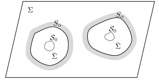
Figure 3: Extension of the manifold: $\Sigma$ is an asymptotically flat space with a boundary $S_{\alpha}$, which is an AGPS with the parameter $\alpha$ (with multiple components, in general). The shaded region is the neighborhood of $S_{\alpha}$ in $\Sigma$, where the local inverse mean curvature flow of Eq. (29) is taken. On $S_{\alpha}$, the manifold $\bar{\Sigma}$ with the metric of Eq. (30) is glued to $\Sigma$. In $\bar{\Sigma}$, a minimal surface ${\cal S}_{0}$ exists at $r=-r_{0}+2\log 2~{}(<0)$ in our current setup.

On (each component of) $S_{\alpha}$, we attach a manifold $\bar{\Sigma}$ with a metric in the range $r\leq 0$ (see Fig. 3),

$$d\bar{s}^{2}=\frac{1-2\exp\left(-\frac{r_{0}}{2}\right)}{1-2\exp\left(-\frac{r+r_{0}}{2}\right)}\exp\left(r\right)\varphi_{0}^{2}(x^{a})dr^{2}+\exp\left(r\right)g_{0,ab}(x^{a})dx^{a}dx^{b},$$ (30)

where $g_{0,ab}:=g_{ab}|_{r=0}$ in the metric of Eq. (29) and $\varphi_{0}=\varphi|_{r=0}$. Each $r$-constant surface is umbilical, i.e., the extrinsic curvature is

$$\bar{k}_{ab}=\frac{1}{2}\bar{k}\bar{g}_{ab}.$$ (31)

Hereafter, quantities with a bar indicate that they are associated with the metric of Eq. (30). The mean curvature and its derivative are

$$\bar{k}=\varphi_{0}^{-1}\sqrt{\frac{1-2\exp\left(-\frac{r+r_{0}}{2}\right)}{1-2\exp\left(-\frac{r_{0}}{2}\right)}\exp\left(-r\right)},$$ (32)

$$\bar{r}^{a}\bar{D}_{a}\bar{k}=-\frac{1}{2}\bar{k}^{2}\frac{1-3\exp\left(-\frac{r+r_{0}}{2}\right)}{1-2\exp\left(-\frac{r+r_{0}}{2}\right)}.$$ (33)

Note that the lapse function in the metric of Eq. (30) has been tuned so that $\bar{k}|_{S_{\alpha}}=k|_{S_{\alpha}}$ is satisfied. Meanwhile, $r_{0}$ is tuned so that

$$\bar{r}^{a}\bar{D}_{a}\bar{k}|_{S_{\alpha}}=\alpha\bar{k}^{2}|_{S_{\alpha}}$$ (34)

holds, which is equivalent to

$$\exp\left(\dfrac{r_{0}}{2}\right)=\frac{3+4\alpha}{1+2\alpha}.$$ (35)

The manifold $\bar{\Sigma}$ is continuously glued to $\Sigma$ at $r=0$ because the induced metrics on the gluing surface $S_{\alpha}$ $(r=0)$ are the same. However, the metric is generally $C^{0}$-class there because $S_{\alpha}$ may not be umbilical, i.e. the extrinsic curvature $k_{ab}$ may have non-vanishing traceless part.

The three-dimensional Ricci scalar of $\bar{\Sigma}$ is expressed with the two-dimensional quantities as

$${}^{(3)}\bar{R}={}^{(2)}\bar{R}-2\bar{\varphi}^{-1}\bar{\cal D}^{2}\bar{\varphi}-2\bar{r}^{a}\bar{D}_{a}\bar{k}-\frac{3}{2}\bar{k}^{2},$$ (36)

where $\bar{\varphi}$ is the lapse function in the metric of Eq. (30), i.e.,

$$\bar{\varphi}=\varphi_{0}(x^{a})\sqrt{\frac{1-2\exp\left(-\frac{r_{0}}{2}\right)}{1-2\exp\left(-\frac{r+r_{0}}{2}\right)}\exp\left(r\right)}.$$ (37)

Each term in the right-hand side of Eq. (36) can be explicitly calculated as

$${}^{(2)}\bar{R}=\exp(-r){}^{(2)}R_{0},\qquad\bar{\varphi}^{-1}\bar{\cal D}^{2}\bar{\varphi}=\exp(-r)\varphi_{0}^{-1}{\cal D}^{2}\varphi_{0},$$

$$2\bar{r}^{a}\bar{D}_{a}\bar{k}+\frac{3}{2}\bar{k}^{2}=\exp(-r)\left(2\alpha+\frac{3}{2}\right)\varphi_{0}^{-2}.$$ (38)

Therefore, we have

$${}^{(3)}\bar{R} = \exp(-r)\left\{{}^{(2)}R_{0}-2\varphi_{0}^{-1}{\cal D}^{2}\varphi_{0}-\left(2\alpha+\frac{3}{2}\right)\varphi_{0}^{-2}\right\}$$ (39)

$$= \exp(-r){}^{(3)}\bar{R}_{0},$$

where ${}^{(3)}\bar{R}_{0}$ is defined by

$${}^{(3)}\bar{R}_{0}:=\lim_{r\nearrow 0}{}^{(3)}\bar{R}.$$ (40)

Since $\varphi_{0}^{-2}=k^{2}|_{r=0}$ holds in the inverse mean curvature flow and $r^{a}D_{a}k|_{r=0}\geq\alpha k^{2}|_{r=0}$ holds from the definition of the AGPS, ${}^{(3)}\bar{R}_{0}$ turns out to be non-negative,

$${}^{(3)}\bar{R}_{0} \geq {}^{(2)}R_{0}-2\varphi_{0}^{-1}{\cal D}^{2}\varphi_{0}-\left.2r^{a}D_{a}k\right|_{r=0}-\left.k^{2}\right|_{r=0}-\left.k_{ab}^{2}\right|_{r=0}$$ (41)

$$= {}^{(3)}R_{0}\geq 0,$$

where ${}^{(3)}R_{0}$ is the Ricci scalar of $\Sigma$ on $S_{\alpha}$ ($r=0$), i.e., ${}^{(3)}R_{0}:=R|_{r=0}$. Thus, the three-dimensional Ricci scalar of the glued manifold $\Sigma\cup\bar{\Sigma}$ is non-negative everywhere. Hence, it is expected that Brays’ proof to the Riemannian Penrose inequality Bray by the conformal flow would be applicable for $\Sigma\cup\bar{\Sigma}$. However, it requires the smoothness of the manifold as an assumption, while our manifold $\Sigma\cup\bar{\Sigma}$ is generally $C^{0}$-class, not $C^{\infty}$-class at the gluing surface. This problem will be fixed later (see Sect. 3.5); in the rest of the present subsection, we assume that Bray’s theorem is applicable to the manifold $\Sigma\cup\bar{\Sigma}$.

The manifold $\bar{\Sigma}$ has a minimal surface at $r=-r_{0}+2\log 2$ (the value of $-r_{0}+2\log 2$ is always negative because of Eq. (35) and $\alpha>-1/2$). The minimal surface is denoted by ${\cal S}_{0}$. From the metric of Eq. (30), we find the direct relation between the area of ${\cal S}_{0}$ and that of $S_{\alpha}$ as

$$A_{0} = \exp(-r_{0}+2\log 2)A_{\alpha}$$ (42)

$$= \left[\frac{2(1+2\alpha)}{3+4\alpha}\right]^{2}A_{\alpha},$$

where $A_{0}$ is the area of ${\cal S}_{0}$. Supposing ${\cal S}_{0}$ to be the outermost minimal surface, the required conditions for which will be discussed in Sect.3.4, the Riemannian Penrose inequality Bray gives

$$A_{0}\leq 4\pi(2Gm)^{2}.$$ (43)

Combining this with Eq. (42), we have

$$A_{\alpha}\leq 4\pi\left(\frac{3+4\alpha}{1+2\alpha}Gm\right)^{2}.$$ (44)

When equality holds in the inequality of Eq. (44), that for the Riemannian Penrose inequality of Eq. (43) holds as well. Then, the manifold has the metric of the time-symmetric slice of a Schwarzschild spacetime. Hence, each of the manifolds $\Sigma$ and $\bar{\Sigma}$ is isometric to a part of it, and in particular, the surface $r=-r_{0}+2\log 2$ is a spherically symmetric minimal surface. Hence, because of the construction of the manifold $\bar{\Sigma}$ whose metric is given in Eq. (30), $S_{\alpha}$ should also be spherically symmetric and must satisfy $r^{a}D_{a}k=\alpha k^{2}$. As a result, equality in the inequality of Eq. (44) holds if and only if $\Sigma$ is the time-symmetric hypersurface of a Schwarzschild spacetime and $S_{\alpha}$ is the spherically symmetric surface with $r^{a}D_{a}k=\alpha k^{2}$.

As stated before, the remaining task is to show that the manifold $\Sigma\cup\bar{\Sigma}$ can be made smooth at the gluing surface $S_{\alpha}$ and ${\cal S}_{0}$ is the outermost minimal surface. We will discuss the latter in Sect. 3.4, and then, prove the former in Sect. 3.5.

3.4 Outermost Minimal Surface

In the previous subsection, we used the assumption that the minimal surface ${\cal S}_{0}$ at $r=-r_{0}+2\log 2$ in the extended manifold $\bar{\Sigma}$ is outermost. Our Theorems are carefully stated to guarantee this assumption, as we explain below.

For simplicity, the study in this section is given for the non-smooth manifold that we constructed in Sect. 3.3, and the non-existence conditions $(i)$ and $(ii)$ are assumed for $S_{\alpha}$, not for each foliation ${\mathfrak{S}}_{r}$. The discussion here must be extended for all smooth manifolds constructed in Sect. 3.5, and we will come back to this point later.

A part of the minimal surface ${\cal S}_{0}$ at $r=-r_{0}+2\log 2$ is not outermost if an outermost minimal surface exists in $r>0$, in $r<0$, or across $r=0$. We examine these three possible cases, one by one. The first possibility is prohibited by the assumption of the theorem that any part of $S_{\alpha}$ is not enclosed by a minimal surface.

The second case is impossible, i.e., we cannot take minimal surfaces in the extended manifold $\bar{\Sigma}$ not touching with the boundary of $\bar{\Sigma}$ except the minimal surface $r=-r_{0}+2\log 2$. To show this using proof by contradiction, let us assume that the second case is possible. Such a surface has maximum $r$ at some points. Then, we can show that the mean curvature $k$ there becomes positive (i.e., non-zero), and thus, it is not a minimal surface, which leads to a contradiction.

Let us begin with a generic discussion of geometry. Suppose we have a codimension one surface $\sigma$ in a manifold and we take the Gaussian normal coordinates in the neighborhood of $\sigma$,

$$dl^{2}=dy^{2}+h_{ij}dx^{i}dx^{j},$$ (45)

where the surface $\sigma$ is supposed to exist at $y=0$ and its unit normal vector is

$$n_{\mu}=\partial_{\mu}y.$$ (46)

We take another surface $\tilde{\sigma}$ characterized with $\tilde{y}=0$ and

$$\tilde{y}=y-\delta y(x^{i}).$$ (47)

Suppose that this surface has maximum $y$ at $x^{i}=0$ and its value is $y=0$. Hence, $\tilde{\sigma}$ is tangent to $\sigma$ at $x^{i}=0$ and the Hessian matrix of $\delta y(x^{i})$ is negative-semidefinite there, i.e. we have

$$\left.\partial_{\mu}\delta y\right|_{x^{i}=0}=0,\qquad\left.h^{ij}\partial_{i}\partial_{j}\delta y\right|_{x^{i}=0}\leq 0.$$ (48)

The unit normal vector of $\tilde{\sigma}$ directing to the same side as $n^{\mu}$ is

$$\tilde{n}_{\mu}=\alpha\partial_{\mu}\tilde{y}.$$ (49)

with

$$\alpha=\bigl{(}1+h^{ij}(\partial_{i}\delta y)(\partial_{j}\delta y)\bigr{)}^{-\frac{1}{2}}.$$ (50)

The induced metric of $\tilde{\sigma}$ is

$$\tilde{h}_{\mu\nu}=g_{\mu\nu}-\tilde{n}_{\mu}\tilde{n}_{\nu},$$ (51)

and $(\tilde{h}_{\mu\nu},\tilde{n}_{\mu})$ coincides with $(h_{\mu\nu},n_{\mu})$ at $x^{i}=0$. The mean curvature of $\tilde{\sigma}$, $\tilde{k}$, is calculated as

$$\tilde{k}:=g^{\mu\nu}\nabla_{\mu}\tilde{n}_{\nu}=g^{\mu\nu}(\partial_{\mu}\alpha)\left(n_{\nu}-\partial_{\nu}\delta y\right)+\alpha g^{\mu\nu}\left(\nabla_{\mu}n_{\nu}-\partial_{\mu}\partial_{\nu}\delta y-\Gamma^{\alpha}_{\mu\nu}\partial_{\alpha}\delta y\right).$$ (52)

Since we have

$$\alpha|_{x^{i}=0}=1,\qquad\left.g^{\mu\nu}\partial_{\mu}\partial_{\nu}\delta y\right|_{x^{i}=0}=h^{ij}\partial_{i}\partial_{j}\delta y,$$

$$\left.\partial_{\mu}\alpha\right|_{x^{i}=0}=\left.-\frac{1}{2}\alpha^{3}\left[2h^{ij}(\partial_{i}\delta y)(\partial_{\mu}\partial_{j}\delta y)+(\partial_{\mu}h^{ij})(\partial_{i}\delta y)(\partial_{j}\delta y)\right]\right|_{x^{i}=0}=0,$$ (53)

the mean curvature $\tilde{k}$ is related to $k$ as

$$\tilde{k}|_{x^{i}=0}=(k-h^{ij}\partial_{i}\partial_{j}\delta y)|_{x^{i}=0}\geq k|_{x^{i}=0},$$ (54)

where we used Eq. (48).

We apply Eq. (54) to surfaces on $\bar{\Sigma}$ as follows. As the surface $\tilde{\sigma}$ and the point $x^{i}=0$, we adopt the minimal surface $\sigma_{m}$ other than $r=-r_{0}+2\log 2$ which is assumed to exist and the point $p_{M}$ where the maximum of $r(=r_{M})$ occurs on the minimal surface, respectively. As the surface $\sigma$, we adopt the $r$-constant surface $r=r_{M}$. Then, from Eq. (54), at $p_{M}$ the mean curvature $k_{m}$ of $\sigma_{m}$ satisfies

$$k_{m}\geq k_{M},$$ (55)

where $k_{M}$ is the mean curvature of the $r=r_{M}$ surface. Since $r_{M}$ is larger than $-r_{0}+2\log 2$, the mean curvature $k_{M}$ is positive, and thus $k_{m}$ should be positive at $p_{M}$. This is inconsistent with the assumption that the surface $\sigma_{m}$ is minimal. Therefore, there exists no minimal surface in $\bar{\Sigma}$ that is not touching with the boundary of $\bar{\Sigma}$ other than $r=-r_{0}+2\log 2$.

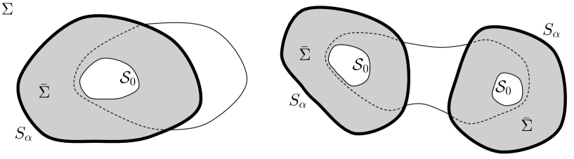
Figure 4: Examples of the third case where ${\cal S}_{0}$ is not the outermost minimal surface: The thick solid curves show the surface $S_{\alpha}$. The outside of $S_{\alpha}$ is $\Sigma$ and the shaded region is $\bar{\Sigma}$. The other boundary of $\bar{\Sigma}$ inside of $S_{\alpha}$ is the minimal surface ${\cal S}_{0}$. Minimal surfaces in $\Sigma$ touching with $S_{\alpha}$, which possibly exist, are shown by solid curves. They might be further extended into $\bar{\Sigma}$ as described with dashed curves. If there exists such a smooth closed minimal surface with a vanishing mean curvature, ${\cal S}_{0}$ is not the outermost minimal surface.

The last possibility may occur in the following situation. In general, there exist minimal surfaces touching with the boundary of $\bar{\Sigma}$. If one of them can be extended to a compact minimal surface in $\Sigma$, we could have a minimal surface enclosing the minimal surface at $r=-r_{0}+2\log 2$ (see Fig. 4). If this occurs, we cannot apply Bray’s theorem to the minimal surface at $r=-r_{0}+2\log 2$.

In our theorem, however, we assume that no minimal surface exists in $\Sigma$ whose area is less than $4\pi(2Gm)^{2}$ and which has a boundary on $S_{\alpha}$. This prevents the situation in Fig. 4 for the following reason. If we have a minimal surface crossing $S_{\alpha}$ like the one shown in Fig. 4, its area has to be smaller than or equal to $4\pi(2Gm)^{2}$ by Bray’s theorem. However, by assumption, the area of its part existing in the domain $\Sigma$ is equal to or larger than $4\pi(2Gm)^{2}$. Hence, the area of the connected minimal surface becomes larger than $4\pi(2Gm)^{2}$, which contradicts Bray’s theorem. This means that such a surface cannot exist.

Summarizing all the discussions above together, the minimal surface at $r=-r_{0}+2\log 2$ is guaranteed to be the outermost one in the $C^{0}$-class manifold constructed in Sect. 3.3. In the next subsection, a sequence of smooth extensions converging to the $C^{0}$-class manifold is constructed. The applicability of the results in this section to them is discussed at the end of Sect. 3.5.

3.5 Smooth Extension

To apply Bray’s proof for the Riemannian Penrose inequality, the manifold should be smooth Bray . However, the constructed manifold $\Sigma\cup\bar{\Sigma}$ in Sect. 3.3 is $C^{0}$-class at the gluing surface, generally. Here, we show that there is a sequence of smooth manifolds with a non-negative Ricci scalar ${}^{(3)}R$ which uniformly converges to $\Sigma\cup\bar{\Sigma}$. On each smooth manifold, we can apply the Riemannian Penrose inequality, and taking the limit, we achieve the inequality of Eq. (43) on $\Sigma\cup\bar{\Sigma}$.

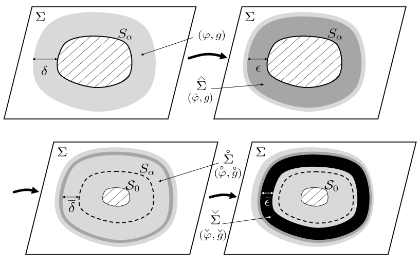
Figure 5: Smooth deformation and extension of the manifold. There are three procedures. The upper-left is the original manifold $\Sigma$. The shaded region is the neighborhood of $S_{\alpha}$ ($\delta>r>0$) where the local inverse mean curvature flow can be taken. In the first procedure, the lapse function is smoothly deformed in $\delta>\epsilon>r>0$, which is described in the upper-right, to make the Ricci scalar ${}^{(3)}R$ strictly positive. The obtained manifold is described by $\hat{\Sigma}$ with the metric $(\hat{\varphi},g)$. In the second procedure, a manifold $\mathring{\Sigma}$ with a metric $(\mathring{\varphi},\mathring{g})$ is attached at $r={\bar{\delta}}$ ($\epsilon>{\bar{\delta}}>0$) to obtain the lower-left manifold. Since the method of gluing the two manifolds is the same as that in Sect. 3.3 except that the gluing position is slightly shifted, the glued manifold is $C^{0}$-class at $r={\bar{\delta}}$. In the third procedure, we smooth the glued manifold by introducing a manifold $\check{\Sigma}$ with the metric $(\check{\varphi},\check{g})$ in the domain ${\bar{\delta}}>r>{\bar{\delta}}-{\bar{\epsilon}}>0$, and a smooth manifold in the lower-right is obtained.

3.5.1 Brief sketch

First, without details, we give a brief sketch on the smooth deformation and extension of the manifold (see Fig. 5) for the proof of Theorem 1. Although Fig. 5 shows one component of $S_{\alpha}$, the smooth deformation and extension should be done for all components of $S_{\alpha}$ simultaneously. We take the foliation of the local inverse mean curvature flow with the metric of Eq. (29) in the neighborhood of $S_{\alpha}$ ($\delta>r>0$). The first procedure is to deform the lapse function $\varphi$ to $\hat{\varphi}$ smoothly in $\delta>\epsilon>r>0$ to make the three-dimensional Ricci scalar strictly positive. The deformed manifold is denoted by $\hat{\Sigma}$ and its deformed metric is written as $(\hat{\varphi},g)$. The second procedure is to consider the $C^{0}$-extension of the manifold in a similar way to that in Sect. 3.3, but the position at which the two manifolds are glued is slightly shifted: We choose the gluing position to be $r={\bar{\delta}}$ ($\epsilon>{\bar{\delta}}>0$), not $r=0$. The extended manifold is denoted by $\mathring{\Sigma}$ with the metric $(\mathring{\varphi},\mathring{g})$, and it uniformly converges to $\bar{\Sigma}$. As seen in Sect. 3.3, $\mathring{\Sigma}$ has the non-negative Ricci scalar everywhere. The third procedure is to introduce a manifold $\check{\Sigma}$ in the domain ${\bar{\delta}}>r>{\bar{\delta}}-{\bar{\epsilon}}>0$, where the metric $(\check{\varphi},\check{g})$ is given by the mixture of $(\hat{\varphi},g)$ of $\hat{\Sigma}$ and $(\mathring{\varphi},\mathring{g})$ of $\mathring{\Sigma}$ so that $\check{\Sigma}$ is smoothly connected to $\hat{\Sigma}$ and $\mathring{\Sigma}$ at $r={\bar{\delta}}$ and $r={\bar{\delta}}-{\bar{\epsilon}}$, respectively. Then, we can show that $\check{\Sigma}$ with the metric $(\check{\varphi},\check{g})$ has the positive Ricci scalar everywhere. Therefore, the obtained manifold, which is the combination of the original manifold in $r\geq\epsilon$, $\hat{\Sigma}$ with the metric $(\hat{\varphi},g)$ in $\epsilon>r\geq{\bar{\delta}}$, $\check{\Sigma}$ with the metric $(\check{\varphi},\check{g})$ in ${\bar{\delta}}>r>{\bar{\delta}}-{\bar{\epsilon}}$, and $\mathring{\Sigma}$ with the metric $(\mathring{\varphi},\mathring{g})$ in ${\bar{\delta}}-{\bar{\epsilon}}\geq r$, is smooth, and has the positive Ricci scalar everywhere. The statements in the previous subsection are applied to the boundary of the deformed region, i.e. the surface ${\mathfrak{S}}_{r}$ at $r=\epsilon$ (denoted by ${\mathfrak{S}}_{\epsilon}$), not to $S_{\alpha}$ (at $r=0$). The sequence of smooth manifolds uniformly converges to $\Sigma\cup\bar{\Sigma}$ in the limit $\epsilon\to 0$. Below, we provide a detailed description. The proof of Theorem 2 can be achieved via a minor change to that of Theorem 1.

3.5.2 The first procedure

We now begin with the detailed proof of Theorem 1. Since the original manifold $\Sigma$ is smooth, we can take a smooth local inverse mean curvature flow H&I ; HP , where $k$ is also a smooth function in the neighborhood of $S_{\alpha}$. Because of the positivity of $k$ on $S_{\alpha}$, $k$ is positive in a sufficiently small neighborhood, $0\leq r<\delta$. Similarly, since $r^{a}D_{a}k$ and $k_{ab}$ are smooth as well, there exists a positive constant $\beta$ satisfying

$$0<2r^{a}D_{a}k+k^{2}+k_{ab}^{2}<\beta k^{2}$$ (56)

everywhere in the neighborhood $0\leq r<\delta$, where we used our assumption, $r^{a}D_{a}k\geq\alpha k^{2}>-(1/2)k^{2}$ on $S_{\alpha}$.

On $S_{\alpha}$, the three-dimensional Ricci scalar ${}^{(3)}R$ is non-negative by assumption. The first procedure is to deform the metric so that ${}^{(3)}R$ becomes strictly positive on and near $S_{\alpha}$. If it is already satisfied, this first procedure is unnecessary and we can skip to the second procedure. Otherwise, we introduce another metric in the region $0\leq r<\epsilon<\delta$ as

$$d\hat{s}^{2} =\hskip 4.2679pt u^{2}(r)\varphi^{2}dr^{2}+g_{ab}dx^{a}dx^{b}$$ (57)

$$=: \hat{\varphi}^{2}dr^{2}+g_{ab}dx^{a}dx^{b},$$

$$u(r) := 1-\exp\left(-\frac{C\delta}{\epsilon-r}\right),$$ (58)

where $C$ is a constant. At $r=\epsilon$, this metric is smoothly connected with the original metric of Eq. (29). The connected smooth manifold is denoted by $\hat{\Sigma}$. This metric uniformly converges to the metric of Eq. (29) in the limit $\epsilon\to 0$. The geometrical quantities with the metric of Eq. (57) on an $r$-constant surface are written as

$${}^{(2)}\hat{R}={}^{(2)}R,\qquad\hat{\varphi}^{-1}\hat{\cal D}^{2}\hat{\varphi}=\varphi^{-1}{\cal D}^{2}\varphi,$$

$$\hat{k}_{ab}=u^{-1}k_{ab},\qquad\hat{k}=u^{-1}k,\qquad\hat{r}^{a}\hat{D}_{a}\hat{k}=-u^{-2}k^{2}(\partial_{r}\log u)+u^{-2}r^{a}D_{a}k,$$ (59)

where we used $\varphi k=1$ in the last equation. Here, the variables with and without hat, such as $\hat{k}$ and $k$, indicate those of the metrics of Eqs. (57) and (29), respectively. The three-dimensional Ricci scalar of the metric of Eq. (57) can be expressed as

$${}^{(3)}\hat{R} = {}^{(2)}\hat{R}-2\hat{\varphi}^{-1}\hat{\cal D}^{2}\hat{\varphi}-2\hat{r}^{a}\hat{D}_{a}\hat{k}-\hat{k}^{2}-\hat{k}_{ab}^{2}$$ (60)

$$= {}^{(3)}R+\left(1-u^{-2}\right)\left(2r^{a}D_{a}k+k^{2}+k_{ab}^{2}\right)+2u^{-2}k^{2}\partial_{r}\log u.$$

The functions involving $u$ in the above equation are estimated as

$$0 > 1-u^{-2}\ =\ u^{-2}\left[-2\exp\left(-\frac{C\delta}{\epsilon-r}\right)+\exp\left(-2\frac{C\delta}{\epsilon-r}\right)\right]$$ (61)

$$> -2u^{-2}\exp\left(-\frac{C\delta}{\epsilon-r}\right),$$

$$\partial_{r}\log u = u^{-1}\frac{C\delta}{(\epsilon-r)^{2}}\exp\left(-\frac{C\delta}{\epsilon-r}\right)\ >\ \frac{C}{\delta}\exp\left(-\frac{C\delta}{\epsilon-r}\right).$$ (62)

These relations, together with Eq. (56), imply

$${}^{(3)}\hat{R}\ >\ {}^{(3)}R+2\frac{k^{2}}{u^{2}}\left(\frac{C}{\delta}-\beta\right)\exp\left(-\frac{C\delta}{\epsilon-r}\right).$$ (63)

Therefore, if we take $C>\beta\delta>0$, ${}^{(3)}\hat{R}$ is strictly positive in the region $0\leq r<\epsilon$. On $S_{\alpha}$, $(\hat{r}^{a}\hat{D}_{a}\hat{k})/\hat{k}^{2}$ is estimated as

$$\left.\frac{\hat{r}^{a}\hat{D}_{a}\hat{k}}{\hat{k}^{2}}\right|_{S_{\alpha}} = \left.\frac{(r^{a}D_{a}k)}{k^{2}}\right|_{S_{\alpha}}-\left.\partial_{r}\log u\right|_{S_{\alpha}}$$ (64)

$$= \left.\frac{(r^{a}D_{a}k)}{k^{2}}\right|_{S_{\alpha}}-\dfrac{C\delta}{\epsilon^{2}}\frac{\exp\left(-\dfrac{C\delta}{\epsilon}\right)}{1-\exp\left(-\dfrac{C\delta}{\epsilon}\right)}$$

$$\geq \alpha+C_{1}\epsilon=:\bar{\alpha},$$

where $C_{1}$ is a (negative) constant.

3.5.3 The second procedure

We now describe the second procedure. We introduce a manifold $\mathring{\Sigma}$ with the following metric:

$$d\mathring{s}^{2} = \frac{1-2\exp\left(-\frac{r_{{\bar{\delta}}}}{2}\right)}{1-2\exp\left(-\frac{r-{\bar{\delta}}+r_{\bar{\delta}}}{2}\right)}\exp\left(r-{\bar{\delta}}\right)\hat{\varphi}_{\bar{\delta}}^{2}(x^{a})dr^{2}+\exp\left(r-{\bar{\delta}}\right)g_{{\bar{\delta}},ab}(x^{a})dx^{a}dx^{b}$$ (65)

$$=: \mathring{\varphi}^{2}dr^{2}+\mathring{g}_{ab}dx^{a}dx^{b},$$

where $\hat{\varphi}_{\bar{\delta}}=\hat{\varphi}|_{r={\bar{\delta}}}$ and $g_{{\bar{\delta}},ab}(x^{a})=g_{ab}|_{r={\bar{\delta}}}$. Here, this metric has one parameter ${\bar{\delta}}$, which is required to satisfy $0<{\bar{\delta}}<\epsilon$, and $r_{\bar{\delta}}$ is determined later. This manifold $\mathring{\Sigma}$ uniformly converges to $\bar{\Sigma}$ in the limit $\epsilon\to 0$ (which leads to ${\bar{\delta}}\to 0$). We glue the two manifolds $\hat{\Sigma}$ and $\mathring{\Sigma}$ along the surface $r={\bar{\delta}}$ denoted by ${\mathfrak{S}}_{\bar{\delta}}$. Since $\hat{r}^{a}\hat{D}_{a}\hat{k}$ and $\hat{k}$ are smooth regular functions in $0<r\leq{\bar{\delta}}$, the relation between the values of $\hat{r}^{a}\hat{D}_{a}\hat{k}/\hat{k}^{2}$ on ${\mathfrak{S}}_{\bar{\delta}}$ and on $S_{\alpha}$ is estimated as

$$\left.\frac{\hat{r}^{a}\hat{D}_{a}\hat{k}}{\hat{k}^{2}}\right|_{{\mathfrak{S}}_{\bar{\delta}}} \geq \left.\frac{\hat{r}^{a}\hat{D}_{a}\hat{k}}{\hat{k}^{2}}\right|_{S_{\alpha}}+\bar{C}_{2}\epsilon$$ (66)

$$\geq \bar{\alpha}+\bar{C}_{2}\epsilon=\alpha+C_{2}\epsilon=:\mathring{\alpha},$$

where $\bar{C}_{2}$ and $C_{2}(=C_{1}+\bar{C}_{2})$ are constants, and $\bar{\alpha}$ is determined in Eq. (64). Note that $\mathring{\alpha}>-1/2$ can be satisfied by taking a sufficiently small $\epsilon$, because $C_{2}$ is a constant independent of $\epsilon$. Similarly to the case of the metric of Eq. (30) in Sect. 3.3, $\mathring{\varphi}$ and $r_{\bar{\delta}}$ are taken so that $\mathring{k}=\hat{k}$ and $(\mathring{r}^{a}\mathring{D}_{a}\mathring{k})=\mathring{\alpha}\mathring{k}^{2}$ are satisfied on ${\mathfrak{S}}_{{\bar{\delta}}}$. Here, the geometric quantities with circles (such as $\mathring{k}$) are those with respect to the metric of Eq. (65). At this point, the obtained manifold, $\mathring{\Sigma}$ glued to $\Sigma$ on ${\mathfrak{S}}_{\bar{\delta}}$, is still $C^{0}$-class, generally.

3.5.4 The third procedure

The third procedure is as follows. Let us deform the glued manifold in the domain ${\bar{\delta}}-{\bar{\epsilon}}<r<{\bar{\delta}}$ to make it smooth, where ${\bar{\epsilon}}$ is any constant satisfying $0<{\bar{\epsilon}}<{\bar{\delta}}$. We consider the difference of the metrics of Eqs. (57) and (65) around ${\mathfrak{S}}_{\bar{\delta}}$. On ${\mathfrak{S}}_{\bar{\delta}}$, the components of the two metrics have been set to be equal to each other. Since $\hat{k}$ and $\mathring{k}$ are equal on ${\mathfrak{S}}_{{\bar{\delta}}}$, the first-order derivative of the metric component proportional to $g_{ab}|_{r={\bar{\delta}}}$ is continuous as well. By contrast, the first-order derivative of the traceless components of the metric is not continuous. Therefore, since each metric is smooth, the difference between them can be written as

$$g_{ab}-\mathring{g}_{ab}=(r-{\bar{\delta}})^{2}T\mathring{g}_{ab}+(r-{\bar{\delta}})h_{ab},\qquad\hat{\varphi}-\mathring{\varphi}=2(r-{\bar{\delta}})\mathring{\varphi}\Phi,$$ (67)

with smooth functions $T$, $h_{ab}$ and $\Phi$, where $h_{ab}$ is traceless, and $\mathring{g}^{ab}h_{ab}=0$. In ${\bar{\delta}}-{\bar{\epsilon}}<r<{\bar{\delta}}$, we consider a manifold with the following smoothed metric:

$$d\check{s}^{2} = \mathring{\varphi}^{2}\left(1+\left[\frac{d}{dr}F^{2}(r)\right]\Phi\right)^{2}dr^{2}+\left(\mathring{g}_{ab}\left[1+F^{2}(r)T\right]+F(r)h_{ab}\right)dx^{a}dx^{b},$$ (68)

$$=: \check{\varphi}^{2}dr^{2}+\check{g}_{ab}dx^{a}dx^{b},$$

where

$$F(r):=(r-{\bar{\delta}})f(r-{\bar{\delta}})$$ (69)

with a function $f(r)$ defined on $-{\bar{\epsilon}}<r<0$ that satisfies

$$\lim_{r\nearrow 0}f(r)=1,\quad\lim_{r\searrow-{\bar{\epsilon}}}f(r)=0,\quad\lim_{r\nearrow 0}f^{(n)}(r)=\lim_{r\searrow-{\bar{\epsilon}}}f^{(n)}(r)=0,$$

$$\left|\frac{d}{dr}(rf)\right|<1,\quad\frac{d^{2}}{dr^{2}}(rf)^{2}<2.$$ (70)

Here, $f^{(n)}$ is the $n$th order derivative of $f$ for an arbitrary positive integer $n$. Note that there exist functions satisfying the above requirements; we show an example in Appendix A. Then, this manifold can be smoothly glued to $\Sigma$ with the metric of Eq. (57) on ${\mathfrak{S}}_{{\bar{\delta}}}$ and $\mathring{\Sigma}$ with the metric of Eq. (65) at $r={\bar{\delta}}-{\bar{\epsilon}}$. Moreover, the obtained manifold uniformly converges to $\Sigma\cup\bar{\Sigma}$ with the metrics of Eqs. (29) and (30) in Sect. 3.3 in the limit $\epsilon\to 0$ (which gives ${\bar{\delta}}\to 0$ and ${\bar{\epsilon}}\to 0$). The metric of Eq. (68) and its derivatives with respect to $r$ are estimated in terms of those of the metric of Eq. (57), as

$$\check{\varphi}=\mathring{\varphi}|_{r={\bar{\delta}}}+{\cal O}({\bar{\delta}}-r),\qquad\check{g}_{ab}=\mathring{g}_{ab}|_{r={\bar{\delta}}}+{\cal O}({\bar{\delta}}-r),$$

$$\check{g}^{ab}=\mathring{g}^{ab}|_{r={\bar{\delta}}}-Fh^{ab}+{\cal O}\left(({\bar{\delta}}-r)^{2}\right),$$

$$\partial_{r}\log\check{\varphi}=(\partial_{r}\log\mathring{\varphi})|_{r={\bar{\delta}}}+(F^{2})^{\prime\prime}\Phi+{\cal O}({\bar{\delta}}-r),$$ (71)

$$\partial_{r}\check{g}_{ab}=(\partial_{r}\mathring{g}_{ab})|_{r={\bar{\delta}}}+(F)^{\prime}h_{ab}+{\cal O}({\bar{\delta}}-r),$$

$$\partial_{r}^{2}\check{g}_{ab}=\left.\left(\partial_{r}^{2}\mathring{g}_{ab}\right)\right|_{r={\bar{\delta}}}+\mathring{g}_{ab}\left(F^{2}\right)^{\prime\prime}T+F^{\prime\prime}h_{ab}+2F^{\prime}\partial_{r}h_{ab}+{\cal O}({\bar{\delta}}-r),$$

where the prime means the derivative with respect to $r$, i.e., $F^{\prime}=dF/dr$, and $h^{ab}:=\mathring{g}^{ac}h_{cd}\mathring{g}^{db}$. Note that the order of $F$, $F^{2}$ and their derivatives are $F={\cal O}({\bar{\epsilon}})$, $F^{\prime}={\cal O}(1)$, $F^{\prime\prime}={\cal O}(1/{\bar{\epsilon}})$, $F^{2}={\cal O}({\bar{\epsilon}}^{2})$, $(F^{2})^{\prime}={\cal O}({\bar{\epsilon}})$, and $(F^{2})^{\prime\prime}={\cal O}(1)$. Then, the geometric quantities are expressed as

$$\check{k}_{ab}=\mathring{k}_{ab}|_{r={\bar{\delta}}}+\frac{F^{\prime}}{2\mathring{\varphi}|_{r={\bar{\delta}}}}h_{ab}+{\cal O}({\bar{\delta}}-r),\qquad\check{k}=\mathring{k}|_{r={\bar{\delta}}}+{\cal O}({\bar{\delta}}-r),$$

$$\check{r}^{a}\check{D}_{a}\check{k}=(\mathring{r}^{a}\mathring{D}_{a}\mathring{k})|_{r={\bar{\delta}}}+(F^{2})^{\prime\prime}\left.\left(\frac{4T-4\mathring{\varphi}\Phi\mathring{k}-h_{ab}^{2}}{4\mathring{\varphi}^{2}}\right)\right|_{r={\bar{\delta}}}+{\cal O}({\bar{\delta}}-r).$$ (72)

$${}^{(2)}\check{R}={}^{(2)}\mathring{R}|_{r={\bar{\delta}}}+{\cal O}({\bar{\delta}}-r),\qquad\check{\varphi}^{-1}\check{\cal D}^{2}\check{\varphi}=\left(\mathring{\varphi}^{-1}\mathring{\cal D}^{2}\mathring{\varphi}\right)\Big{|}_{r={\bar{\delta}}}+{\cal O}({\bar{\delta}}-r),$$

where the geometric functions with check marks (such as $\check{k}$) are those with respect to the metric of Eq. (68). Note that we used the traceless condition of $h_{ab}$, i.e. $\mathring{g}^{ab}h_{ab}=0$, to simplify the expressions. The three-dimensional Ricci scalar for the metric of Eq. (68) is reduced to

$${}^{(3)}\check{R}={}^{(3)}\mathring{R}|_{r={\bar{\delta}}}-F^{\prime 2}\left.\left(\frac{1}{2\mathring{\varphi}}h_{ab}\right)^{2}\right|_{r={\bar{\delta}}}-\left(F^{2}\right)^{\prime\prime}\left.\left(\frac{4T-4\mathring{\varphi}\Phi\mathring{k}-h_{ab}^{2}}{2\mathring{\varphi}^{2}}\right)\right|_{r={\bar{\delta}}}$$

$$\hskip 312.9803pt+{\cal O}({\bar{\delta}}-r),$$ (73)

where we used $\mathring{k}^{ab}h_{ab}=0$ since $r=\mathrm{constant}$ surfaces are umbilical for the metric of Eq. (65). Here, we evaluate the value of the three-dimensional Ricci scalar ${}^{(3)}\hat{R}$ for the metric of Eq. (57) (i.e. on $\hat{\Sigma}$) on $r={\bar{\delta}}$. Since ${}^{(3)}\check{R}$ and ${}^{(3)}\hat{R}$ have the same value on $r={\bar{\delta}}$, we have

$${}^{(3)}\hat{R}|_{r={\bar{\delta}}}={}^{(3)}\mathring{R}|_{r={\bar{\delta}}}-\left.\left(\frac{1}{2\mathring{\varphi}}h_{ab}\right)^{2}\right|_{r={\bar{\delta}}}-\left.\left(\frac{4T-4\mathring{\varphi}\Phi\mathring{k}-h_{ab}^{2}}{\mathring{\varphi}^{2}}\right)\right|_{r={\bar{\delta}}},$$ (74)

using $F^{\prime}=1$ and $(F^{2})^{\prime\prime}=2$ at $r={\bar{\delta}}$. In the same way, we have

$$\left.\left(\hat{r}^{a}\hat{D}_{a}\hat{k}\right)\right|_{r={\bar{\delta}}}=\left.\left(\mathring{r}^{a}\mathring{D}_{a}\mathring{k}\right)\right|_{r={\bar{\delta}}}+\left.\left(\frac{4T-4\mathring{\varphi}\Phi\mathring{k}-h_{ab}^{2}}{2\mathring{\varphi}^{2}}\right)\right|_{r={\bar{\delta}}}.$$ (75)

Since

$$\left.\frac{\hat{r}^{a}\hat{D}_{a}\hat{k}}{\hat{k}^{2}}\right|_{r={\bar{\delta}}}\geq\mathring{\alpha}=\left.\frac{\mathring{r}^{a}\mathring{D}_{a}\mathring{k}}{\mathring{k^{2}}}\right|_{r={\bar{\delta}}}\qquad\mbox{and}\qquad\hat{k}=\mathring{k}$$ (76)

are satisfied from the construction of the metric of Eq. (65), we have

$$\left(4T-4\mathring{\varphi}\Phi\mathring{k}-h_{ab}^{2}\right)\Big{|}_{r={\bar{\delta}}}\geq 0.$$ (77)

Using the above and the inequalities of Eq. (70), we find

$${}^{(3)}\check{R} = {}^{(3)}\hat{R}|_{r={\bar{\delta}}}+\left(1-F^{\prime 2}\right)\left.\left(\frac{1}{2\mathring{\varphi}}h_{ab}\right)^{2}\right|_{r={\bar{\delta}}}$$ (78)

$$\hskip 28.45274pt+\left[2-\left(F^{2}\right)^{\prime\prime}\right]\left.\left(\frac{4T-4\mathring{\varphi}\Phi\mathring{k}-h_{ab}^{2}}{2\mathring{\varphi}^{2}}\right)\right|_{r={\bar{\delta}}}+{\cal O}({\bar{\delta}}-r)$$

$$\geq {}^{(3)}\hat{R}|_{r={\bar{\delta}}}+{\cal O}({\bar{\epsilon}}).$$

Since ${}^{(3)}\hat{R}|_{r={\bar{\delta}}}$ is strictly positive, ${}^{(3)}\check{R}$ can be made positive everywhere by setting ${\bar{\epsilon}}$ to be a sufficiently small value. In other words, there is a critical value ${\bar{\epsilon}}_{c}$ such that ${}^{(3)}\check{R}$ becomes non-negative for ${\bar{\epsilon}}\leq{\bar{\epsilon}}_{c}$. As a result, there exists a sequence of smooth manifolds with a non-negative Ricci scalar, which uniformly converges to $\Sigma\cup\bar{\Sigma}$ with the metrics of Eqs. (29) and (30).

3.5.5 Reconsideration of Sect. 3.4

We should confirm that the discussion in Sect. 3.4 is applicable in the sequence of the smooth manifolds constructed above. If the boundary of the deformed region is ${\mathfrak{S}}_{\epsilon}$ (see Fig. 7), the discussion in Sect. 3.4 should be applied for ${\mathfrak{S}}_{\epsilon}$, instead of $S_{\alpha}$. For $r<\epsilon$ in any constructed smooth manifold, the mean curvature $k$ on each $r$-constant surface is positive. By taking $\epsilon<\varepsilon$, where $\varepsilon$ is introduced in Theorem 1, the surface ${\mathfrak{S}}_{\epsilon}$ at $r=\epsilon$ does not have minimal surfaces satisfying conditions (i) and (ii) by the assumption of Theorem 1. Therefore, the result in Sect. 3.4 holds for the constructed smooth manifold. Then, by taking the limit $\epsilon\to 0$, the proof of Theorem 1 is completed.

3.5.6 Proof of Theorem. 2

With respect to Theorem 2, no assumptions for each leaf of the foliation exist. Instead, a smooth inward extension from $S_{\alpha}$ is assumed to exist, and the local mean curvature flow is also assumed to be taken in the interior of $S_{\alpha}$. In the proof of Theorem 1, the deformation occurs in the range $0<r<\epsilon$, where the local inverse mean curvature flow is taken, and the outer boundary of the smooth deformation is located at $r=\epsilon$, i.e., ${\mathfrak{S}}_{\epsilon}$. In the setting of Theorem 2, on the other hand, since the existence of the local mean curvature flow in the interior of $S_{\alpha}$, i.e., $r<0$, is assumed, the deformation based on the local mean curvature flow can be done in the range $-\epsilon<r<0$ (see Fig. 7 and compare between Figs. 7 and 7). Then, its outer boundary is located exactly at $r=0$, i.e., $S_{\alpha}$. Such a deformation can be achieved in the same way as that of Theorem 1, but the coordinate $r$ in the proof of Theorem 1 is replaced by a new coordinate $s$ defined as $r=s-\epsilon$. The analysis is carried out by replacing $r$ in the proof of Theorem 1 by $s$, thus the outer boundary of the deformed region is located at $s=\epsilon$, which is $S_{\alpha}$. The result in Sect. 3.4 is applicable without change, and taking the limit $\epsilon\to 0$ gives Theorem 2.

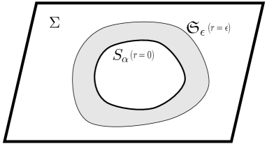
Figure 6: Deformed region in Theorem 1: The deformed region is shown as the gray one. The thick and thin curves correspond to $S_{\alpha}$ ($r=0$) and ${\mathfrak{S}}_{\epsilon}$ ($r=\epsilon$), respectively. The local mean curvature flow is taken in exterior of $S_{\alpha}$. The smooth deformation is done for $0<r<\epsilon$, and the outer boundary of the deformed region is located at $r=\epsilon$, that is ${\mathfrak{S}}_{\epsilon}$.

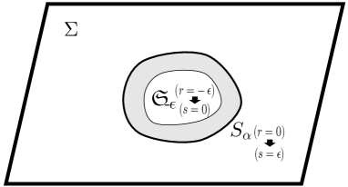
Figure 7: Deformed region in Theorem 2: The gray-colored part shows the deformed region. The thick and thin curves correspond to $S_{\alpha}$ ($r=0$) and ${\mathfrak{S}}_{-\epsilon}$ ($r=-\epsilon$), respectively. By assumption, the local mean curvature flow can be taken in the interior of $S_{\alpha}$ ($-\epsilon<r<0$). The smooth deformation can be done there and the boundary of deformed region can be $S_{\alpha}$.

4 Summary

In this paper, we have introduced a new concept, the attractive gravity probe surface (AGPS), to characterize the strengths of gravitational field. An AGPS is a two-dimensional closed surface that satisfies $k>0$ and $r^{a}D_{a}k/k^{2}\geq\alpha$ for the local inverse mean curvature flow, where $\alpha$ is a constant satisfying $\alpha>-1/2$. This concept can be applied to surfaces in regions with various strength of the gravitational field, including weak-gravity regions: The parameter $\alpha$ controls the strength of the gravitational field. For instance, for $r$-constant surfaces in a $t$-constant slice of a Schwarzschild spacetime, $r^{a}D_{a}k/k^{2}$ is a monotonically decreasing continuous function of $r$. It converges to $\infty$ in the limit where the surface approaches the horizon, while it converges to $-1/2$ at spatial infinity. Hence, $\alpha$ is interpreted as an indicator for the minimum strength of the gravitational field on the surface, because it gives the lower bound of $r^{a}D_{a}k/k^{2}$ on that surface.

Then, we have generalized the Riemannian Penrose inequality to the areal inequality for AGPSs; for asymptotically flat or AdS spaces, the area of an AGPS surface has an upper bound, $A_{\alpha}\leq 4\pi[(3+4\alpha)/(1+2\alpha)]^{2}(Gm)^{2}$ (the exact statement is presented in Sect. 2.2 and as Theorem 1 in Sect. 3.2). In the limit $\alpha\to\infty$ and in the case $\alpha=0$, our inequality is reduced to the Riemannian Penrose inequality and its analog for the LTS, respectively. The proof for asymptotically flat spaces is carried out by applying Bray’s theorem derived using the conformal flow. This means that our inequality is applicable to the case of an AGPS with multiple components. For asymptotically AdS spaces, our argument relied on the Geroch monotonicity in the inverse mean curvature flow. The proof for the areal inequality for AGPSs based on the conformal flow, which requires the generalization of Bray’s method to AdS spaces, will be an important remaining problem.

It would be interesting to extend our inequality to that in Einstein-Maxwell systems, as in the case of the Riemannian Penrose inequality Jang:1979zz ; Weinstein:2004uu ; Khuri:2013ana ; Khuri:2014wqa and its analog for the LTS Lee:2020pre . Moreover, the extension to the higher-dimensional cases is expected to be possible for asymptotically flat spaces. We leave these topics for future works.

It is also important to consider the relation to the behavior of photons and the possible connection to observations. For LTSs, the relations to dynamically transversely trapping surfaces, which is a generalization of the concept of the photon surface for generic spacetimes based on the photon orbits, have been discussed Lee:2020pre ; Yoshino:2017gqv ; Yoshino:2019dty ; Yoshino:2019mqw . It would be interesting to explore the relation between the AGPSs and the photon behavior.

Appendix A An example of the matching function $f$

An example of the matching function is

$$f(r)=\left(1+\exp x(r)\right)^{-1},\qquad x(r):=\frac{{\bar{\epsilon}}}{r}+\frac{{\bar{\epsilon}}}{r+{\bar{\epsilon}}}+1,$$ (79)

defined on $-{\bar{\epsilon}}<r<0$. The behavior of $f$, $(rf)^{\prime}$ and $[(rf)^{2}]^{\prime\prime}$ is shown in Fig. 8, where the prime means the derivative with respect to $r$ (not to $x$), i.e., $f^{\prime}=\frac{d}{dr}f\bigl{(}x(r)\bigr{)}$. From this figure, one can expect that the requirements of Eq. (70) would be satisfied. Here, we provide a solid proof for this fact.

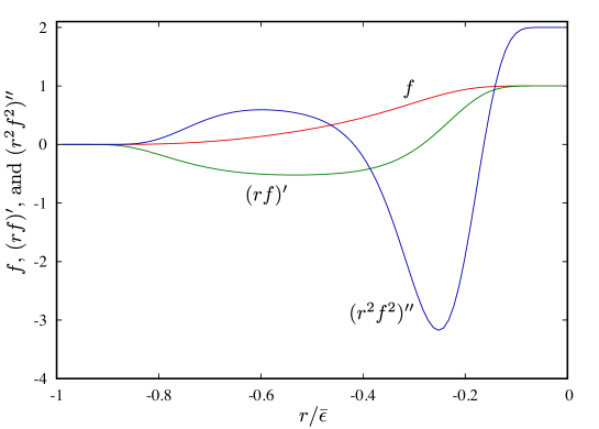
Figure 8: The behavior of the functions $f$, $(rf)^{\prime}$, and $(r^{2}f^{2})^{\prime\prime}$ for the matching function given by Eq. (79).

A.1 Evaluation of the first three equations of conditions of Eq. (70)

It is trivial that the first two equations of Eq. (70) are satisfied because of

$$\lim_{r\nearrow 0}e^{x}=0,\quad\lim_{r\searrow-{\bar{\epsilon}}}e^{x}=\infty.$$ (80)

Since the function $f$ converges to $1$ and $0$ very rapidly in the limit of $r\nearrow 0$ and $r\searrow-{\bar{\epsilon}}$, respectively, the third equation of Eq. (70) is expected to be satisfied. Let us show it exactly.

The $n$th-order derivatives of $f(x(r))$ with respect to $r$ are written by the finite sum of terms, each of which has the form

$$c_{l}\frac{d^{m}f}{dx^{m}}\prod_{k=1}^{m}\frac{d^{a_{k}}x}{dr^{a_{k}}},$$ (81)

where $m$ is a positive integer, $c_{l}$ is a constant and the $a_{k}$ terms are positive integers satisfying

$$n=\sum_{k=1}^{m}a_{k}.$$ (82)

Different $a_{k}$ terms may take the same integer. The third equation of Eq. (70) holds if each term of Eq. (81) converges to zero in the limits $r\nearrow 0$ and $r\searrow-{\bar{\epsilon}}$.

The $a_{k}$th-order derivatives of $x(r)$ become

$$\dfrac{d^{a_{k}}x}{dr^{a_{k}}}=(-1)^{a_{k}}{a_{k}}!\left(\dfrac{1}{r^{{a_{k}}+1}}+\dfrac{1}{(r+{\bar{\epsilon}})^{{a_{k}}+1}}\right){\bar{\epsilon}}.$$ (83)

Around $r=0$, the absolute value of it is bounded from above as

$$\left|\dfrac{d^{a_{k}}x}{dr^{a_{k}}}\right|<c_{a_{k}}\left|\dfrac{1}{r^{{a_{k}}+1}}\right|,$$ (84)

where $c_{a_{k}}$ is a positive constant. Thus, the absolute value of the product of the derivatives of $x$ in Eq. (81) is bounded from above as

$$\prod_{k=1}^{m}\left|\frac{d^{a_{k}}x}{dr^{a_{k}}}\right|<c_{a}\left|\dfrac{1}{r^{a+m}}\right|,\qquad\mbox{where}\qquad c_{a}:=\prod_{k=1}^{m}c_{k},\qquad a:=\sum_{k=1}^{m}a_{k}.$$ (85)

We now estimate the $m$th-order derivative of $f(x(r))$ with respect to $x$. The first-order derivative is calculated as

$$\dfrac{df}{dx}=f(f-1).$$ (86)

Defining a functional space $\cal F$ as

$${\cal F}:=\left\{f(f-1)p(f)\left|\mbox{$p(f)$ is a polynomial of $f$}\right.\right\},$$ (87)

we show

$$\frac{d^{m}f}{dx^{m}}\in{\cal F}$$ (88)

for $m\geq 1$ by the method of induction. For $m=1$, it is true because of Eq. (86). Suppose Eq. (88) is satisfied for $m=q$. The assumption indicates that $d^{q}f/dx^{q}$ is written by $f(f-1)p_{q}(f)$ with a polynomial $p_{q}(f)$, and its derivative becomes

$$\frac{d^{q+1}f}{dx^{q+1}}=f(f-1)\left[(2f-1)p_{q}(f)+\frac{dp_{q}(f)}{df}\right]\in{\cal F}.$$ (89)

Therefore, Eq. (88) is proved for arbitrary $m\geq 1$.

Now, we know that each $m$th-order derivative is written as

$$\frac{d^{m}f}{dx^{m}}=f(f-1)p_{m}(f),$$ (90)

with a polynomial $p_{m}(f)$. The function $f$ converges to unity in the limit $r\nearrow 0$. Therefore, $|fp_{m}(f)|$ is bounded from above by a positive constant $\tilde{c}_{m}$ around $r=0$. On the other hand, $|f-1|$ is estimated around $r=0$ as

$$|f-1|=\frac{\exp x}{1+\exp x}<\bar{c}_{m}\exp x=\bar{c}_{m}\exp\left(\frac{{\bar{\epsilon}}}{r}+\frac{{\bar{\epsilon}}}{r+{\bar{\epsilon}}}+1\right)<\bar{c}_{m}\exp\left(\frac{{\bar{\epsilon}}}{r}\right),$$ (91)

with a positive constant $\bar{c}_{m}$. Therefore, we have

$$\left|\frac{d^{m}f}{dx^{m}}\right|<\tilde{c}_{m}\bar{c}_{m}\exp\left(\frac{{\bar{\epsilon}}}{r}\right)=:c_{m}\exp\left(\frac{{\bar{\epsilon}}}{r}\right),$$ (92)

around $r=0$. As a result, Eq. (81) is estimated around $r=0$ as

$$\left|c_{l}\frac{d^{m}f}{dx^{m}}\prod_{k=1}^{l}\frac{d^{a_{k}}x}{dr^{a_{k}}}\right|<\left|c_{l}\right|c_{a}c_{m}\left|\dfrac{1}{r^{a+l}}\right|\exp\left(\frac{{\bar{\epsilon}}}{r}\right)\xrightarrow[r\nearrow 0]{}0.$$ (93)

This leads to

$$\lim_{r\nearrow 0}f^{(n)}(r)=0.$$ (94)

In a similar way, we can show the vanishing of $f^{(n)}(r)$ for the limit $r\searrow-{\bar{\epsilon}}$.

A.2 Estimate of $(rf)^{\prime}$

We now show that the condition $|(rf)^{\prime}|<1$ is satisfied. First, we show the upper bound of $(rf)^{\prime}$ as follows:

$$(rf)^{\prime} = \dfrac{1}{1+e^{x}}\left[1+\dfrac{r{\bar{\epsilon}}e^{x}}{1+e^{x}}\left(\dfrac{1}{r^{2}}+\dfrac{1}{(r+{\bar{\epsilon}})^{2}}\right)\right]<\dfrac{1}{1+e^{x}}\ <\ 1.$$ (95)

Note that $f(r)$ is defined on $-{\bar{\epsilon}}<r<0$, i.e., $r$ is negative.

Next, we estimate the lower bound of $(rf)^{\prime}$ in the cases of $-{{\bar{\epsilon}}}/{2}\leq r<0$ and $-{\bar{\epsilon}}<r\leq-{{\bar{\epsilon}}}/{2}$, separately. It is useful to express $(rf)^{\prime}$ as follows:

$$(rf)^{\prime} = \frac{1}{1+e^{x}}\left\{1+\frac{e^{x}}{1+e^{x}}\left[x-\left(\frac{{\bar{\epsilon}}}{{\bar{\epsilon}}+r}\right)^{2}-1\right]\right\}$$ (96)

$$= \frac{1}{1+e^{x}}\left\{1+\frac{e^{x}}{1+e^{x}}\left[x-\left(x-\frac{{\bar{\epsilon}}}{r}-1\right)^{2}-1\right]\right\}.$$ (97)

A.2.1 The case $-{{\bar{\epsilon}}}/{2}\leq r<0$

In this case, we have the inequalities

$$x\leq 1,\qquad e^{x}\leq e,\qquad 1<\frac{{\bar{\epsilon}}}{{\bar{\epsilon}}+r}\leq 2.$$ (98)

From Eq. (96), $(rf)^{\prime}$ is bounded as

$$(rf)^{\prime}>\frac{1}{1+e^{x}}\left[1+\frac{e^{x}}{1+e^{x}}(x-5)\right].$$ (99)

The derivative of the right-hand side of the above is

$$\dfrac{d}{dx}\left(\frac{1}{1+e^{x}}\left[1+\frac{e^{x}}{1+e^{x}}(x-5)\right]\right)=\frac{e^{x}(1-e^{x})}{(1+e^{x})^{3}}(x-5).$$ (100)

This is negative for $x<0$ and positive for $0<x\leq 1$. Thus, the minimum of the right-hand side of Eq. (99) occurs at $x=0$, and hence, we have

$$(rf)^{\prime}\geq\frac{1}{1+1}\left[1+\frac{1}{1+1}(-5)\right]=-\frac{3}{4}>-1.$$ (101)

A.2.2 The case $-{\bar{\epsilon}}<r\leq-{{\bar{\epsilon}}}/{2}$

In this case, we have

$$x\geq 1,\qquad e^{x}\geq e,\qquad 1<-\frac{{\bar{\epsilon}}}{r}\leq 2.$$ (102)

From Eq. (97), the lower bound is evaluated as

$$(rf)^{\prime} \geq \frac{1}{1+e^{x}}\left\{1+\frac{e^{x}}{1+e^{x}}\left[x-\left(x+1\right)^{2}-1\right]\right\}$$ (103)

$$= \frac{1}{(1+e^{x})^{2}}\left[1-e^{x}\left(x^{2}+x+1\right)\right]$$

$$> -\frac{1}{(1+e^{-x})^{2}}e^{-x}\left(x^{2}+x+1\right).$$

Since

$$\frac{d}{dx}\left[e^{-x}\left(x^{2}+x+1\right)\right]=-e^{x}x(x-1)<0$$ (104)

holds, $e^{-x}\left(x^{2}+x+1\right)$ is a decreasing function for $x>1$. Meanwhile, ${1}/{(1+e^{-x})^{2}}$ is an increasing function. Then, $(rf)^{\prime}$ is found to be bounded from below as

$$(rf)^{\prime}>-\left[\frac{1}{(1+e^{-x})^{2}}\right]\Big{|}_{x=2}\left[e^{-x}\left(x^{2}+x+1\right)\right]|_{x=1}>-1$$ (105)

for $1<x<2$, and

$$(rf)^{\prime}>-\left[\frac{1}{(1+e^{-x})^{2}}\right]\Big{|}_{x\to\infty}\left[e^{-x}\left(x^{2}+x+1\right)\right]|_{x=2}>-1$$ (106)

for $2<x$.

A.3 Estimate of $\left[(rf)^{2}\right]^{\prime\prime}$

The second-order derivative of $(rf)^{2}$ can be written as

$$\left[(rf)^{2}\right]^{\prime\prime}=\frac{2}{(1+e^{x})^{4}}\left\{(1+e^{x})^{2}+2e^{x}(1+e^{x})\left[x-1-\left(\frac{{\bar{\epsilon}}}{{\bar{\epsilon}}+r}\right)^{3}\right]\right.$$

$$\hskip 156.49014pt\left.+e^{x}\left(2e^{x}-1\right)\left[x-1-\left(\frac{{\bar{\epsilon}}}{{\bar{\epsilon}}+r}\right)^{2}\right]^{2}\right\}.$$ (107)

We will show that $\left[(rf)^{2}\right]^{\prime\prime}<2$ is satisfied, in the three cases, $e^{x}\leq 1/2$ (i.e. $x\leq-\log 2$), $1/2<e^{x}\leq e$ (i.e. $-7/10<-\log 2<x\leq 1$), and $e<e^{x}$ (i.e. $1<x$), separately.

A.3.1 The case $e^{x}\leq 1/2$  (i.e. $x\leq-\log 2$)

Since $x$ and $(2e^{x}-1)$ are negative, Eq. (107) gives

$$\left[(rf)^{2}\right]^{\prime\prime}\leq\frac{2}{(1+e^{x})^{4}}(1+e^{x})^{2}<1.$$ (108)

A.3.2 The case $1/2<e^{x}\leq e$  (i.e. $-7/10<-\log 2<x\leq 1$)

We can express ${{\bar{\epsilon}}}/{r}$ in terms of ${{\bar{\epsilon}}}/{(r+{\bar{\epsilon}})}$ as

$$\frac{{\bar{\epsilon}}}{r}=\frac{{\bar{\epsilon}}}{r+{\bar{\epsilon}}}\left(1-\frac{{\bar{\epsilon}}}{r+{\bar{\epsilon}}}\right)^{-1},$$ (109)

and then, we can see a relation between ${{\bar{\epsilon}}}/{(r+{\bar{\epsilon}})}$ and $x$,

$$\left(\frac{{\bar{\epsilon}}}{r+{\bar{\epsilon}}}\right)^{2}=(x+1)\frac{{\bar{\epsilon}}}{r+{\bar{\epsilon}}}-(x-1).$$ (110)

The terms including ${{\bar{\epsilon}}}/{(r+{\bar{\epsilon}})}$ in the right-hand side of Eq. (107) are rewritten as

$$-\left(\frac{{\bar{\epsilon}}}{r+{\bar{\epsilon}}}\right)^{3}=-\left(x^{2}+x+2\right)\frac{{\bar{\epsilon}}}{r+{\bar{\epsilon}}}+x^{2}-1,$$ (111)

$$\left[\left(\frac{{\bar{\epsilon}}}{r+{\bar{\epsilon}}}\right)^{2}-(x-1)\right]^{2}=\left(x^{3}-x^{2}+3x+5\right)\frac{{\bar{\epsilon}}}{r+{\bar{\epsilon}}}-x^{3}+3x^{2}-7x+5.$$ (112)

Solving Eq. (110) for ${{\bar{\epsilon}}}/{(r+{\bar{\epsilon}})}$, it is estimated as

$$\frac{7}{5}<\frac{{\bar{\epsilon}}}{r+{\bar{\epsilon}}}=\frac{(x+1)+\sqrt{(x-1)^{2}+4}}{2}\leq 2,$$ (113)

where we used $1<{{\bar{\epsilon}}}/{(r+{\bar{\epsilon}})}$ to choose the sign in the front of the square root and $-7/10<x\leq 1$. As a consequence, we find

$$\left[(rf)^{2}\right]^{\prime\prime} = \frac{2}{(1+e^{x})^{4}}\biggl{\{}1+\left(x^{3}-x^{2}+9x-7\right)e^{x}+\left(-2x^{3}+8x^{2}-12x+7\right)e^{2x}$$ (114)

$$\hskip 28.45274pt+\left[-\left(x^{3}+x^{2}+5x+9\right)+\left(2x^{3}-4x^{2}+4x+6\right)e^{x}\right]e^{x}\frac{{\bar{\epsilon}}}{r+{\bar{\epsilon}}}\biggr{\}}$$

$$= \frac{2}{(1+e^{x})^{4}}\biggl{\{}1+\left(x^{3}-x^{2}+9x-7\right)e^{x}+\left(-2x^{3}+8x^{2}-12x+7\right)e^{2x}$$

$$\hskip 56.9055pt+\left[-\left(3x^{2}+3x+6\right)+\left(x^{3}-2x^{2}+2x+3\right)(2e^{x}-1)\right]e^{x}\frac{{\bar{\epsilon}}}{r+{\bar{\epsilon}}}\biggr{\}}$$

$$< \frac{2}{(1+e^{x})^{4}}\biggl{\{}1+\left(x^{3}-x^{2}+9x-7\right)e^{x}+\left(-2x^{3}+8x^{2}-12x+7\right)e^{2x}$$

$$\hskip 56.9055pt+\left[-\frac{7}{5}\left(3x^{2}+3x+6\right)+2\left(x^{3}-2x^{2}+2x+3\right)(2e^{x}-1)\right]e^{x}\biggr{\}}$$

$$= \frac{2}{(1+e^{x})^{4}}\left[1+\left(-x^{3}-\frac{6}{5}x^{2}+\frac{4}{5}x-\frac{107}{5}\right)e^{x}+\left(2x^{3}-4x+19\right)e^{2x}\right].$$

For $-7/10<x\leq 0$, we have $e^{x}\leq 1$ and then $\left[(rf)^{2}\right]^{\prime\prime}$ is bounded from above as

$$\left[(rf)^{2}\right]^{\prime\prime} \leq \frac{2}{(1+e^{x})^{4}}\left[1+\left(-x^{3}-\frac{6}{5}x^{2}+\frac{4}{5}x-\frac{107}{5}\right)e^{x}+\left(2x^{3}-4x+19\right)e^{x}\right]$$ (115)

$$= \frac{2}{(1+e^{x})^{4}}\left[1+\left(x^{3}-\frac{6}{5}x^{2}-\frac{16}{5}x-\frac{12}{5}\right)e^{x}\right]$$

$$< \frac{2}{(1+e^{x})^{4}}\ <\ 2.$$

For $0<x\leq 1$, we have $e^{x}\leq e<3$, and it gives

$$\left[(rf)^{2}\right]^{\prime\prime} < \frac{2}{(1+e^{x})^{4}}\left[1+\frac{1}{3}\left(-x^{3}-\frac{6}{5}x^{2}+\frac{4}{5}x-\frac{107}{5}\right)e^{2x}+\left(2x^{3}-4x+19\right)e^{2x}\right]$$ (116)

$$= \frac{2}{(1+e^{x})^{4}}+\frac{2e^{2x}}{15(1+e^{x})^{4}}\left[25x^{3}-6x^{2}-56x+178\right].$$

The part in the square bracket of the second term in the second line is positive in the interval $0<x\leq 1$ since its function has a minimal value at $x=(6+2\sqrt{1059})/75~{}(<1)$ and a maximal value at $x=(6-2\sqrt{1059})/75~{}(<0)$. Then, the maximum value in $0<x\leq 1$ is under 178. Moreover, we can estimate its coefficient as

$$\frac{2e^{2x}}{15(1+e^{x})^{4}}<\frac{1}{120},$$ (117)

where we used the fact that ${e^{2x}}/{(1+e^{x})^{4}}$ monotonically decreases for $x>0$.

Then, $\left[(rf)^{2}\right]^{\prime\prime}$ is evaluated as

$$\left[(rf)^{2}\right]^{\prime\prime} < \frac{2}{(1+e^{x})^{4}}+\dfrac{178}{120}$$ (118)

$$< \dfrac{1}{8}+\dfrac{178}{120}\ <\ 2$$

A.3.3 The case $e<e^{x}$  (i.e. $1<x$)

We estimate the first and second lines of Eq. (114). The terms in the square bracket in the second line are shown to be positive as

$$-\left(x^{3}+x^{2}+5x+9\right)+\left(2x^{3}-4x^{2}+4x+6\right)e^{x}$$

$$\hskip 28.45274pt=-\left(x^{3}+x^{2}+5x+9\right)+2\left[x(x-1)^{2}+x+3\right]e^{x}$$

$$\hskip 28.45274pt>-\left(x^{3}+x^{2}+5x+9\right)+5\left[x(x-1)^{2}+x+3\right]$$

$$\hskip 28.45274pt=4x^{3}-11x^{2}+5x+6>0,$$ (119)

where we used $5/2<e<e^{x}$ and $x>1$ in the first inequality and used $x>1$ in the second inequality. Since for $x>1$ we have ${{\bar{\epsilon}}}/{(r+{\bar{\epsilon}})}<x+1$ [see Eq. (113)], the value of $\left[(rf)^{2}\right]^{\prime\prime}$ is bounded as

$$\left[(rf)^{2}\right]^{\prime\prime} < \frac{2}{(1+e^{x})^{4}}\left\{1+\left(x^{3}-x^{2}+9x-7\right)e^{x}+\left(-2x^{3}+8x^{2}-12x+7\right)e^{2x}\right.$$ (120)

$$\hskip 56.9055pt\left.+\left[-\left(x^{3}+x^{2}+5x+9\right)+\left(2x^{3}-4x^{2}+4x+6\right)e^{x}\right]e^{x}(1+x)\right\}$$

$$= \frac{2}{(1+e^{x})^{4}}\left\{1-\left(x^{4}+x^{3}+7x^{2}+5x+16\right)e^{x}\right.$$

$$\hskip 113.81102pt\left.+\left(2x^{4}-4x^{3}+8x^{2}-2x+13\right)e^{2x}\right\}$$

$$< \frac{2}{(1+e^{x})^{4}}+\frac{2e^{2x}}{(1+e^{x})^{4}}\left(2x^{4}-4x^{3}+8x^{2}-2x+13\right).$$

Here, the first term has the maximum value $2(1+e)^{-4}<1/50$ at $x=1$. The derivative of the second term is shown to be negative as

$$\frac{d}{dx}\left[\frac{2e^{2x}}{(1+e^{x})^{4}}\left(2x^{4}-4x^{3}+8x^{2}-2x+13\right)\right]$$

$$\hskip 56.9055pt=\frac{4e^{2x}}{(1+e^{x})^{5}}\left[\left(2x^{4}+2x^{2}+6x+12\right)-e^{x}\left(2x^{4}-8x^{3}+14x^{2}-10x+14\right)\right]$$

$$\hskip 56.9055pt<\frac{4e^{2x}}{(1+e^{x})^{5}}\biggl{[}\left(2x^{4}+2x^{2}+6x+12\right)$$

$$\hskip 142.26378pt-\left(1+x+\frac{1}{2}x^{2}\right)\left(2x^{4}-8x^{3}+14x^{2}-10x+14\right)\biggr{]}$$

$$\hskip 56.9055pt=-\frac{4e^{2x}}{(1+e^{x})^{5}}\left[\left(x^{3}-x^{2}-x-1\right)^{2}+x(x-1)(x+4)+3x^{2}+1\right]<0,$$ (121)

where we used

$$2x^{4}-8x^{3}+14x^{2}-10x+14=2(x-2)^{2}x^{2}+5(x-1)^{2}+x^{2}+9>0$$ (122)

and $e^{x}>1+x+x^{2}/2$. Thus, the second term of the right-hand side of Eq. (120) is a decreasing function. The maximum of the right-hand side of the inequality of Eq. (120) occurs at $x=1$ and its value satisfies

$$\frac{34e^{2}}{(1+e)^{4}}<\frac{14}{10}.$$ (123)

Therefore, the value of $\left[(rf)^{2}\right]^{\prime\prime}$ is less than 2.

References

- (1) R. Penrose, Annals N. Y. Acad. Sci. 224, 125 (1973).
- (2) P. S. Jang and R. M. Wald, J. Math. Phys. 18, 41 (1977).
- (3) G. Huisken and T. Ilmanen, J. Diff. Geom. 59, 353 (2001).
- (4) H. Bray, J. Differential Geom., 59 (2001), 177-267.
- (5) T. Shiromizu, Y. Tomikawa, K. Izumi and H. Yoshino, PTEP 2017 (2017) no.3, 033E01.
- (6) R. Geroch, Ann. N.Y. Acad. Sci. 224, 108 (1973).
- (7) W. Boucher, G. W. Gibbons and G. T. Horowitz, Phys. Rev. D 30, 2447 (1984).
- (8) G. W. Gibbons, Class. Quant. Grav. 16, 1677 (1999).
- (9) L. F. Abbott and S. Deser, Nucl. Phys. B 195, 76-96 (1982).
- (10) A. Ashtekar and A. Magnon, Class. Quant. Grav. 1, L39-L44 (1984).
- (11) S. Aminneborg, I. Bengtsson, S. Holst and P. Peldan, Class. Quant. Grav. 13, 2707-2714 (1996)
- (12) G. Huisken, A. Polden (1999) Geometric evolution equations for hypersurfaces. In: Hildebrandt S., Struwe M. (eds) Calculus of Variations and Geometric Evolution Problems. Lecture Notes in Mathematics, vol 1713. Springer, Berlin, Heidelberg.
- (13) P. S. Jang, Phys. Rev. D 20, 834-838 (1979).
- (14) G. Weinstein and S. Yamada, Commun. Math. Phys. 257, 703-723 (2005).
- (15) M. Khuri, G. Weinstein and S. Yamada, Contemp. Math. 653, 219-226 (2015).
- (16) M. Khuri, G. Weinstein and S. Yamada, J. Diff. Geom. 106, no.3, 451-498 (2017).
- (17) K. Lee, T. Shiromizu, H. Yoshino, K. Izumi and Y. Tomikawa, PTEP 2020, no.10, 103E03 (2020).
- (18) H. Yoshino, K. Izumi, T. Shiromizu and Y. Tomikawa, PTEP 2017, no.6, 063E01 (2017).
- (19) H. Yoshino, K. Izumi, T. Shiromizu and Y. Tomikawa, PTEP 2020, no.2, 023E02 (2020).
- (20) H. Yoshino, K. Izumi, T. Shiromizu and Y. Tomikawa, PTEP 2020, no.5, 053E01 (2020).