The Pathway Elaboration Method for Mean First Passage Time Estimation in Large Continuous-Time Markov Chains with Applications to Nucleic Acid Kinetics

Abstract

For predicting the kinetics of nucleic acid reactions, continuous-time Markov chains (CTMCs) are widely used. The rate of a reaction can be obtained through the mean first passage time (MFPT) of its CTMC. However, a typical issue in CTMCs is that the number of states could be large, making MFPT estimation challenging, particularly for events that happen on a long time scale (rare events). We propose the pathway elaboration method, a time-efficient probabilistic truncation-based approach for detailed-balance CTMCs. It can be used for estimating the MFPT for rare events in addition to rapidly evaluating perturbed parameters without expensive recomputations. We demonstrate that pathway elaboration is suitable for predicting nucleic acid kinetics by conducting computational experiments on 267 measurements that cover a wide range of rates for different types of reactions. We utilize pathway elaboration to gain insight on the kinetics of two contrasting reactions, one being a rare event. We then compare the performance of pathway elaboration with the stochastic simulation algorithm (SSA) for MFPT estimation on 237 of the reactions for which SSA is feasible. We further build truncated CTMCs with SSA and transition path sampling (TPS) to compare with pathway elaboration. Finally, we use pathway elaboration to rapidly evaluate perturbed model parameters during optimization with respect to experimentally measured rates for these 237 reactions. The testing error on the remaining 30 reactions, which involved rare events and were not feasible to simulate with SSA, improved comparably with the training error. Our framework and dataset are available at https://github.com/DNA-and-Natural-Algorithms-Group/PathwayElaboration.

T1Joint first authorship for first two authors: Sedigheh Zolaktaf and Frits Dannenberg contributed equally to this work.

, , , , and

1 Introduction

Predicting the kinetics of reactions involving interacting nucleic acid strands is desirable for building autonomous nanoscale devices whose nucleic acid sequences and experimental conditions need to be carefully designed to control their behaviour, such as RNA toehold switches (Angenent-Mari et al., 2020) and oscillators (Srinivas et al., 2017). By kinetics, we mean non-equilibrium dynamics, such as the rate of a reaction and the order in which different strands interact when a system is not in thermodynamic equilibrium. Accurate and efficient prediction methods would facilitate the design of complex molecular devices by reducing, though not eliminating, the need for debugging deficiencies with wet-lab experiments.

The kinetics of nucleic acid reactions are often modeled as continuous-time Markov chains (CTMC) with elementary steps (Schaeffer, Thachuk and Winfree, 2015; Flamm et al., 2000; Dykeman, 2015). A CTMC is a stochastic process on a discrete set of states that have the Markov property so that future possible states are independent of past states given the current state. The time in a state before transitioning to another state, the holding time, is continuous; to retain the Markov property, holding times follow an exponential distribution with a single rate parameter for each state-to-state transition. In elementary step models of nucleic acid kinetics, states correspond to secondary structures and a transition between two states corresponds to the breaking or forming of a base pair. The transition rates are specified with kinetic models (Metropolis et al., 1953) along with thermodynamic models (Hofacker, 2003; Zadeh et al., 2011). We call the states corresponding to the reactants and the products of a reaction as initial states and target states, respectively.

A fundamental kinetic property of interest in a nucleic acid reaction is the reaction rate constant. We can estimate the rate using the mean first passage time (MFPT) to reach the set of target states starting from the set of initial states in the CTMC  (Schaeffer, 2013). The MFPT is commonly used to estimate the rate of a process (Schaeffer, 2013; Reimann, Schmid and Hänggi, 1999; Singhal, Snow and Pande, 2004). For a CTMC with a reasonable state space size, a matrix equation can provide an exact solution to the MFPT (Suhov and Kelbert, 2008). However, direct application of matrix methods is not feasible for CTMCs that have large state spaces. In this work we are interested in two computational challenges when the state space is too large to allow exact matrix methods. The first challenge is efficiently estimating MFPTs for reactions that happen on long time scale (rare events) and the second challenge is efficiently recalculating MFPTs for mildly perturbed model parameters. Next we describe these challenges and then we describe our contributions.

For large state spaces researchers may resort to stochastic simulations (Gillespie, 2007; Ripley, 2009; Asmussen and Glynn, 2007; Doob, 1942; Gillespie, 1977). For CTMCs in particular, the stochastic simulation algorithm (SSA) (Doob, 1942; Gillespie, 1977) is a widely used Monte Carlo procedure that can numerically generate statistically correct trajectories. By trajectory, we mean a path from one state to another state, plus a holding time at each state along the path. By sampling enough trajectories from the initial states to the target states, an estimate of the MFPT can be obtained. However, SSA is inefficient for estimating MFPTs of rare events, that is reactions that happen on a long time scales, such as reactions that involve high-energy barrier states. A number of techniques have been developed for efficient sampling of simulation trajectories relevant to the event of interest (Bolhuis et al., 2002; Allen, Valeriani and ten Wolde, 2009; Rubino and Tuffin, 2009). Such sampling techniques, unfortunately, must generally be re-run if model parameters change, which makes it costly to perform parameter scans or to optimize a model.

Alternatively, large CTMCs can be approximated by models with just a subset of “most relevant” states, in order to estimate MFPTs and other properties of interest with matrix methods (Munsky and Khammash, 2006; Kuntz et al., 2019; Singhal, Snow and Pande, 2004). In truncated-based models, a set of most relevant states is selected, and transitions are added between selected states that are adjacent in the original CTMC. Methods have also been developed for reusing truncated models under mildly perturbed conditions such as temperature (Singhal, Snow and Pande, 2004). The key challenge here is to efficiently enumerate a suitable subset of states that are sufficient for accurate estimation and also few enough that the matrix methods are tractable. As we discuss further in our related work section, the methods to date fail to do this for applications such as MPFT estimation of nucleic acid reactions that are rare events.

Here we are interested in a method that successfully addresses both challenges for MFPT estimation in large CTMCs: rare events and efficient recomputation for perturbed model parameters. We develop a method which uses both biased and local stochastic simulations to build truncated CTMCs relevant to a (possibly rare) event of interest. With extensive experiments we demonstrate that our method is suitable for predicting nucleic acid kinetics modeled as CTMCs with elementary steps. Although in this work we only evaluate our method in the context of nucleic acid kinetics, we believe it could also be useful in other applications of detailed-balance CTMCs, such as chemical reaction networks (Anderson and Kurtz, 2011) and protein folding (McGibbon and Pande, 2015).

Our contributions. In Section 4, we propose the pathway elaboration method for estimating MFPTs in detailed-balance CTMCs. Pathway elaboration is a time-efficient probabilistic truncation-based approach which can be used for MFPT estimation of rare events and also enables the rapid evaluation of perturbed parameters. In pathway elaboration, we first construct a pathway by biasing SSA simulations from the initial states to the targets states. The biased simulations are guaranteed to reach the target states in expected time that is linear in the distance from initial to target states. Then, we expand the pathway by running SSA simulations for a limited time from every state of the pathway, with the intention of increasing accuracy by increasing representation throughout the pathway. Finally, we compute all possible transitions between the sampled states that were not encountered in the previous two steps. For the resulting truncated CTMC, we solve a matrix equation to compute the MFPT to the target state (or states). Since solving matrix equations could be slow for large CTMCs, pathway elaboration includes a $\delta$-pruning step to efficiently prune CTMCs while keeping MFPT estimates within predetermined upper bounds. In this way, solving the system for other parameter settings becomes faster. Figure 1 illustrates the pathway elaboration method and its applications.

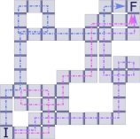
(a) Pathway construction

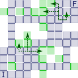
(b) State elaboration

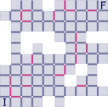
(c) Transition construction

(d) $\delta$-pruning

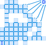
(e) Updating perturbed parameters

(f) Parameter estimation

(g) Obtain functionality

Figure 1: The pathway elaboration method and its applications. Pathway elaboration makes possible MFPT estimation of rare events and the rapid evaluation of perturbed parameters. Here, in the underling detailed-balance CTMC, boxes in a square grid represent states of the CTMC, with transitions between adjacent boxes, initial state I at bottom left and target state F at top right. (a) From state I, sample paths that are biased towards the target state F. Three sampled paths are shown with blue, pink and purple dotted lines. (b) From each sampled state found in the previous step, run short unbiased simulations to fill in the neighborhood. Simulations from two states are shown with green dashed lines. The green states and transitions are sampled. (c) Include all missing transitions between the states that were sampled in steps a and b. The red transitions are included. (d) Prune states that are expected to reach the target state quickly by redirecting their transitions into a new state. (e) For perturbed model parameters, keep the topology of the truncated CTMC, but update the transition rates. (f) We can use truncated CTMCs for perturbed parameters, such as to estimate model parameters or (g) to predict forward $(k_{+})$ and reverse $(k_{-})$ reaction rate constants as temperature changes.

To evaluate pathway elaboration, we focus on predicting the kinetics of nucleic acids. We implement the method using the Multistrand kinetic simulator (Schaeffer, 2013; Schaeffer, Thachuk and Winfree, 2015). Multistrand provides a secondary-structure level model of the folding kinetics of multiple interacting nucleic acid strands, with thermodynamic energies consistent with NUPACK (Zadeh et al., 2011) and a stochastic simulation method based on SSA. The challenges of large state spaces, rare events, and handling perturbed parameters all arise for nucleic acid kinetics. Since the number of secondary structures may be exponentially large in the length of the strands, applying matrix equations is infeasible. Also, SSA often takes a long time to complete for rare nucleic acid reactions. Moreover, the rapid evaluation of mildly perturbed parameters is required, for example to calibrate the underlying kinetic model or to obtain a desired functionality (see Figures 1f and 1g). We conduct computational experiments on a dataset of 267 nucleic acid kinetics (Bonnet, Krichevsky and Libchaber, 1998; Cisse, Kim and Ha, 2012; Hata, Kitajima and Suyama, 2018; Zhang et al., 2018; Machinek et al., 2014) (described in Section 5.1). The dataset consists of various types of reactions, such as helix association and toehold-mediated three-way strand displacement, for which experimentally measured reaction rate constants vary over 8.6 orders of magnitude. We partition the 267 reactions into two sets, 237 where SSA is feasible for MPFT estimation, i.e., completes within two weeks, and the remaining 30 for which SSA is not feasible.

In our experiments, first in Section 5.3, we conduct a case study and use pathway elaboration to gain insight on the kinetics of two contrasting reactions, one being a rare event. Then, in Section 5.4, to evaluate the estimations of pathway elaboration, first, we compare them with estimations obtained from SSA for the 237 feasible reactions that were feasible with SSA. We use SSA since obtaining MFPTs with matrix equations is not possible for many of these reactions and SSA provides statistically correct trajectories. We find that for the settings we use, the mean absolute error (MAE) of the $\log_{10}$ reaction rate constant (or equivalently the MAE of the $\log_{10}$ MFPT) is $0.13$. This is a reasonable accuracy since the $\log_{10}$ reaction constant predictions of SSA vary over $7.7$ orders of magnitude (see Figure 6). In our experiments, pathway elaboration is on average 5 times faster than SSA on these reactions. Furthermore, to evaluate the estimations of pathway elaboration, we build truncated CTMCs using simulations from SSA and transition path sampling (TPS) (Bolhuis et al., 2002; Singhal, Snow and Pande, 2004; Eidelson and Peters, 2012). In our experiments, the MAE of pathway elaboration with SSA simulations compares well with the MAE of SSA-based truncated CTMCs with SSA simulations. Moreover, the truncated CTMCs built with TPS have a larger MAE with SSA than pathway elaboration with SSA and the estimations have a larger variance. Finally, in Section 5.5, we use pathway elaboration to rapidly evaluate perturbed model parameters during optimization of Multistrand kinetic parameters. We use the same 237 reactions for training the optimizer and the remaining 30 as our testing set. Using the optimized parameters, pathway elaboration estimates of reaction rate constants on our dataset are greatly improved over the estimates using non-optimized parameters. For the training set, the MAE of the $\log_{10}$ reaction rate constants of pathway elaboration with experimental measurements reduces from $1.43$ to $0.46$, that is, a $26.9$-fold error in the reaction rate constant reduces to a $2.8$-fold error on average. The MAE over the 30 remaining reactions – which involve rare events and have large state spaces – reduces from $1.13$ to $0.64$, that is, a $13.4$-fold error in the reaction rate constant reduces to a $4.3$-fold error on average. On average for these 30 reactions, pathway elaboration takes less than two days, whereas SSA is not feasible within two weeks. The entire optimization and evaluation takes less than five days.

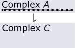
(a) Hairpin closing

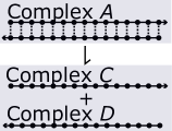
(b) Helix dissociation

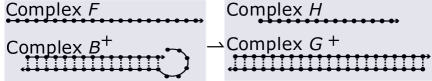
(c) Toehold-mediated three-way strand displacement

Figure 2: Examples of unimolecular and bimolecular interacting nucleic acid strand reactions. (a) Hairpin closing is a unimolecular reaction. It has one reactant complex ($A$) and one product complex ($C$). The reverse reaction, hairpin opening, is also a unimolecular reaction. (b) Helix dissociation is a unimolecular reaction. It has one reactant complex ($A$) and two product complexes ($C$ and $D$). The reverse reaction, helix association, is a bimolecular reaction. (c) Toehold-mediated three-way strand displacement is a bimolecular reaction. It has two reactant complexes ($B$ and $F$) and two product complexes ($G$ and $H$).

2 Related Work

There exist numerous Monte Carlo techniques (Rubino and Tuffin, 2009) for driving simulations towards the target states or to reduce the variance of estimators. For example, importance sampling techniques (Hajiaghayi et al., 2014; Doucet and Johansen, 2009) use an auxiliary sampler to bias simulations, after which estimates are corrected with importance weights. Moreover, many accelerated variants of SSA have been developed for CTMC models of chemically reacting systems  (Gillespie, 2007; Cao, Gillespie and Petzold, 2007; Gillespie, 2001), which can be adapted to simulate arbitrary CTMCs. There also exists a proliferation of rare event simulation methods for molecular dynamics (Zuckerman and Chong, 2017; Allen, Valeriani and ten Wolde, 2009; Bolhuis et al., 2002). The ideas behind these methods can be adapted for CTMCs and can be used along with SSA for more efficient computations. For example, in transition path sampling (TPS) (Bolhuis et al., 2002) an ensemble of paths are generated using a Monte Carlo procedure. First, a single path is generated that connects the initial and target states. New paths are then generated by picking random states along the current paths and running time-limited simulations from the states. Sampled states along paths that do not reach the initial or target states are rejected. Even though we could use TPS along with SSA to simulate rare events for CTMCs (Eidelson and Peters, 2012), it is likely that many of the simulated paths require a long simulation time. For example, if the energy landscape has more than one local maximum between the initial and target states, then paths simulated from in between these local maxima could require a long simulation time to reach either the initial or the target states. Moreover, the simulated paths could be correlated and depend on the initial path, and therefore the estimations of different runs could have a high variance. The correlation of paths could be reduced by retaining a fraction of the paths but it would also reduce the computational efficiency.

Stochastic simulations are usually not reusable for the rapid evaluation of perturbed parameters and have to be adapted. This is because the holding times of simulated trajectories need to be updated, which requires that information about all transitions from each sampled state is also stored. With the pathway elaboration method we can rapidly evaluate perturbed parameters by updating transition rates of the truncated CTMC. Stochastic simulation methods have been to some extent adapted for the rapid evaluation of perturbed parameters. SSA has been adapted in the fixed path ensemble inference (FPEI) approach (Zolaktaf et al., 2019) for parameter estimation. In this approach, an ensemble of paths are generated using SSA and are then compacted and reused for mildly perturbed parameters. To estimate MFPTs, a Monte Carlo approach is used based on expected holding times of states. Despite being useful for parameter estimation in general, this method is not suitable for rare events, because the paths are generated according to SSA. In Section 5.4.3, we use SSA to build truncated CTMCs for MFPT estimation and we compare its performance with pathway elaboration.

An alternative to sampling methods is to develop a smaller CTMC, whose MFPT well approximates that of the original large CTMC model. As is the case with sampling methods, techniques that have been developed to approximate the continuous state spaces of molecular dynamics simulations can be adapted for this purpose. In the context of predicting protein folding kinetics, the collection of paths produced by TPS has been used to build a so-called Markovian state model (MSM) (Singhal, Snow and Pande, 2004). The MSM is the CTMC obtained by including all states and transitions along the sampled paths; since each state appears once, the MSM is more compact then the underlying set of paths. The MSM approach can easily be adapted to build approximations to large CTMC models, for the purpose of estimating MFPTs and other properties of the CTMC. The resulting MSM is a truncated CTMC. That is, it contains a subset of the states of the original CTMC, with transitions between states that are adjacent in the original CTMC. Our pathway elaboration approach is similar to this approach in that sampled paths are used to build a truncated CTMC. However, in pathway elaboration, we have a state elaboration step that helps model low-energy basins that might have a big influence on MFPTs in a complex landscape with multiple barriers and/or deep basins. Since the CTMCs in our application of predicting nucleic acid kinetics satisfy detailed balance, the initial and final states are still reachable from all states in the CTMC and so the MFPT is still finite when these additional states are included. In Section 5.4.3, we use TPS to build truncated CTMCs for MFPT estimation and we compare its performance with pathway elaboration.

Another important problem in CTMCs is computing transient probabilities, that is the probability distribution of the states over time. Transient probabilities can be computed exactly with the master equation (Van Kampen, 1992) for CTMCs that have a feasible state space size. An important tool that has been developed to quantify the error of transient probability estimations for truncated CTMCs is the finite state projection (FSP) method (Munsky and Khammash, 2006). The FSP method tells us that as the size of the state space of the truncated CTMC grows, the approximation monotonically improves and provides upper and lower bounds on the true transient probabilities. In Section 4, we show how we can adapt the FSP method to quantify the error of MFPT estimates for truncated CTMCs. As the authors of the FSP method mention, there are many ways to grow the state space, for example by iteratively adding states that are reachable from the already-included states within a fixed number of steps. There have been many attempts to enumerate a suitable set of states that provides good approximations while being small enough that transient probabilities can be computed efficiently (Dinh and Sidje, 2016). In the Krylov-FSP-SSA approach (Sidje and Vo, 2015) an SSA approach is used to drive the FSP and adaptive Krylov methods are used to efficiently evaluate the matrix exponential for transient probability estimation. In brief, the method starts from an initial state space and proceeds iteratively in three steps. First, it drops states that have become improbable. Second, it runs SSA from each state of the remaining state space to incorporate probable states. Third, it adds states that are reachable within a fixed number of steps. Despite its great potential, this way of building the state space may not be suitable for estimating MFPTs of rare events. The pathway elaboration method is similar to this approach in the sense that it uses SSA in the state elaboration step. However, the pathway elaboration method uses biased simulations to reach target states efficiently.

The Krylov-FSP-SSA method has also been used to build truncated CTMCs for the purpose of optimizing parameter sets that are used for transient probability estimation (Dinh and Sidje, 2017). Moreover, in related work (Georgoulas, Hillston and Sanguinetti, 2017), an ensemble of truncated CTMCs is used to obtain an unbiased estimator of transient probabilities, which are further used for Bayesian inference.

A probabilistic roadmap is another type of graph-based model, related to our work (Kavraki et al., 1996; Tang et al., 2005). States in a probabilistic roadmap can be selected by random sampling or according to relevant properties, such as having low free energy. Then edges are added to connect nearby (though not necessarily adjacent) states. However, there are some challenges with this method that make it unsuitable for our purposes. First, it is not clear that sampling methods based on state (as opposed to path) properties will include important states on the most likely folding trajectories from initial to target states. Another challenge is determining appropriate transition rates between states that are not adjacent in the CTMC model. Instead, we rely on biased sampling of paths from initial to target states.

3 Background

In this section, we first describe the continuous-time Markov chain (CTMC) model to which our pathway elaboration method (Section 4) applies and also provide related definitions. Then we explain how nucleic acid kinetics can be modeled using CTMCs with the Multistrand kinetic model (Schaeffer, 2013; Schaeffer, Thachuk and Winfree, 2015) which is background for our experiments (Section 5).

Continuous-time Markov chain (CTMC). We indicate a CTMC as a tuple $\mathcal{C}=(\mathcal{S},\mathbf{K},\mathbf{\pi}_{0},\mathcal{S}_{\mathrm{target}}$), where $\mathcal{S}$ is a countable set of states, $\mathbf{K}:\mathcal{S}\times\mathcal{S}\rightarrow\mathbb{R}_{\geq 0}$ is the rate matrix and $\mathbf{K}(s,s)=0$ for $s\in\mathcal{S}$, $\mathbf{\pi}_{0}:\mathcal{S}\rightarrow[0,1]$ is the initial state distribution in which $\sum_{s\in\mathcal{S}}\mathbf{\pi}_{0}(s)=1$, and $\mathcal{S}_{\mathrm{target}}$ is the set of target states. We define the set of initial states as $\mathcal{S}_{\mathrm{init}}=\left\{s\in\mathcal{S}~{}\middle|~{}\mathbf{\pi}_{0}(s)\neq 0\right\}.$ For CTMCs considered here, $\mathcal{S}_{\mathrm{target}}\cap\mathcal{S}_{\mathrm{init}}=\emptyset$. A transition between states $s,s^{\prime}\in\mathcal{S}$ can occur only if $\mathbf{K}(s,s^{\prime})>0$. The probability of moving from state $s$ to state $s^{\prime}$ is defined by the transition probability matrix ${\mathbf{P}}:\mathcal{S}\times\mathcal{S}\rightarrow[0,1]$ where

$$\mathbf{P}(s,s^{\prime})=\frac{\mathbf{K}(s,s^{\prime})}{\mathbf{E}(s,s)}.$$ (1)

Here $\mathbf{E}:\mathcal{S}\times\mathcal{S}\rightarrow\mathbb{R}_{\geq 0}$ is a diagonal matrix in which $\mathbf{E}(s,s)=\sum_{s^{\prime}\in\mathcal{S}}\mathbf{K}(s,s^{\prime})$ is the exit rate. The time spent in state $s$ before a transition is triggered is exponentially distributed with exit rate $\mathbf{E}(s,s)$. The generating matrix $\mathbf{Q}:\mathcal{S}\times\mathcal{S}\rightarrow\mathbb{R}$ is $\mathbf{Q}=\mathbf{K}-\mathbf{E}$.

Detailed-balance CTMC. In a detailed-balance CTMC $\mathcal{C}^{R}=(\mathcal{S},\mathbf{K},\mathbf{\pi}_{0},\mathcal{S}_{\mathrm{target}},\mathbf{\pi})$, also known as a reversible CTMC, a probability distribution $\mathbf{\pi}:\mathcal{S}\rightarrow[0,1]$ over the states exists that satisfies the detailed balance condition $\mathbf{\pi}(s)\mathbf{K}(s,s^{\prime})=\mathbf{\pi}(s^{\prime})\mathbf{K}(s^{\prime},s)$ for all $s,s^{\prime}\in\mathcal{S}$. The detailed balance condition is a sufficient condition for ensuring that $\mathbf{\pi}$ is a stationary distribution ($\mathbf{\pi}\mathbf{P}=\mathbf{\pi}$). For a detailed-balance finite-state CTMC, $\mathbf{\pi}$ is the unique stationary distribution of the chain and is also the unique equilibrium distribution (Whitt, 2006).

Boltzmann distribution. In many Markov models of physical systems, eventually the population of states will stabilize and reach a Boltzmann distribution (Schaeffer, Thachuk and Winfree, 2015; Flamm et al., 2000; Tang, 2010) at equilibrium. With this distribution, the probability that a system is in a state $s$ is

$$\mathbf{\pi}(s)=\frac{1}{Z}e^{-\frac{E(s)}{k_{B}T}},$$ (2)

where $E(s)$ is the energy of the system at state $s$, $T$ is the temperature, $k_{B}$ is the Boltzmann constant, and $Z=\sum_{s\in\mathcal{S}}e^{-\frac{E(s)}{k_{B}T}}$ is the partition function. To ensure that at equilibrium states are Boltzmann distributed, the detailed balance conditions are

$$\frac{\mathbf{K}(s,s^{\prime})}{\mathbf{K}(s^{\prime},s)}=e^{-\frac{E(s^{\prime})-E(s)}{K_{B}T}}.$$ (3)

Reversible transition. In this work, a reversible transition between states $s$ and $s^{\prime}$ means $\mathbf{K}(s,s^{\prime})>0$ if and only if $\mathbf{K}(s^{\prime},s)>0$.

Trajectories and paths. A trajectory $(s_{0},t_{0}),(s_{1},t_{1},),...,(s_{m},t_{m},)$ with $m$ transitions over a CTMC $\mathcal{C}=(\mathcal{S},\mathbf{K},\mathbf{\pi}_{0},\mathcal{S}_{\mathrm{target}})$ is a sequence of states $s_{i}$ and holding times $t_{i}$ for which $\mathbf{K}(s_{i},s_{i+1})>0$ and $t_{i}\in\mathbb{R}_{>0}$ for $i\geq 0$. We define a path $s_{0},s_{1},...,s_{m}$ with $m$ transitions over a CTMC $\mathcal{C}=(\mathcal{S},\mathbf{K},\mathbf{\pi}_{0},\mathcal{S}_{\mathrm{target}})$ as a sequence of states $s_{i}$ for which $\mathbf{K}(s_{i},s_{i+1})>0$.

The stochastic simulation algorithm (SSA). SSA (Gillespie, 1977; Doob, 1942) simulates statistically correct trajectories over a CTMC $\mathcal{C}=(\mathcal{S},\mathbf{K},\mathbf{\pi}_{0},\mathcal{S}_{\mathrm{target}})$. At state $s_{i}$, the probability of sampling $s_{i+1}$ is $\mathbf{P}(s_{i},s_{i+1})$. At a jump from state $s_{i}$, it samples the holding time $T_{i}$ from an exponential distribution with exit rate $\mathbf{E}(s,s)=\sum_{s^{\prime}\in\mathcal{S}}\mathbf{K}(s,s^{\prime})$.

Mean first passage time (MFPT). In a CTMC $\mathcal{C}=(\mathcal{S},\mathbf{K},\mathbf{\pi}_{0},\mathcal{S}_{\mathrm{target}})$, for a state $s\in\mathcal{S}$ and a target state $s_{\text{f}}\in\mathcal{S}_{\mathrm{target}}$, the MFPT $\tau_{s}$ is the expected time to first reach $s_{\text{f}}$ starting from state $s$. For state $s$, the MFPT from $s$ to $s_{\text{f}}$ equals the expected holding time in state $s$ plus the MFPT to $s_{\text{f}}$ from the next visited state (Suhov and Kelbert, 2008), so

$$\tau_{s}=\frac{1}{\mathbf{E}(s,s)}+\sum_{s^{\prime}\in\mathcal{S}}\frac{\mathbf{K}(s,s^{\prime})}{\mathbf{E}(s,s)}\tau_{s^{\prime}}.$$ (4)

Multiplying the equation by the exit rate $\mathbf{E}(s,s)=\sum_{s^{\prime}\in\mathcal{S}}\mathbf{K}(s,s^{\prime})$ then yields

$$\sum_{s^{\prime}\in\mathcal{S}}\mathbf{K}(s,s^{\prime})(\tau_{s^{\prime}}-\tau_{s})=-1.$$ (5)

Now writing $\mathbf{t}:\mathcal{S}\setminus s_{\text{f}}\rightarrow\mathbb{R}_{\geq 0}$ to be the vector of MFPTs for each state, such that $\mathbf{t}[s]=\tau_{s}$, we find a matrix equation as

$$\tilde{\mathbf{Q}}\mathbf{t}=-\mathbf{1},$$ (6)

where $\tilde{\mathbf{Q}}$ is obtained from ${\mathbf{Q}}$ by eliminating the row and column corresponding to the target state, and $\mathbf{1}$ is a vector of ones. If there exists a path from every state to the final state $s_{\text{f}}$, then $\tilde{\mathbf{Q}}$ is a weakly chained diagonally dominant matrix and is non-singular (Azimzadeh and Forsyth, 2016). The MFPT from the initial states to the target state $s_{\text{f}}$ is found as

$$\tau_{\mathbf{\pi}_{0}}=\sum_{s\in\mathcal{S}}\mathbf{\pi}_{0}(s)\tau_{s}.$$ (7)

If instead of a single target state $s_{\text{f}}$ we have a set of target states $\mathcal{S}_{\mathrm{target}}$, then to compute the MFPT to $\mathcal{S}_{\mathrm{target}}$ we convert all target states into one state $s_{\text{f}}$ so that $\mathcal{S}^{*}=\mathcal{S}\setminus\mathcal{S}_{\mathrm{target}}\cup\left\{s_{\text{f}}\right\}$. For $s,s^{\prime}\in\mathcal{S}^{*}\setminus\left\{s_{\text{f}}\right\}$, we update the rate matrix $\mathbf{K}^{*}:\mathcal{S}^{*}\rightarrow\mathbb{R}_{\geq 0}$ by $\mathbf{K}^{*}(s,s_{\text{f}})=\sum_{s^{\prime\prime}\in\mathcal{S}_{\mathrm{target}}}\mathbf{K}(s,s^{\prime\prime})$, $\mathbf{K}^{*}(s,s^{\prime})=\mathbf{K}(s,s^{\prime})$, and $\mathbf{K}^{*}(s_{\text{f}},s)$ is not used in the computation of the MFPT (see Eq. 6).

Truncated CTMC. Let $\hat{\mathcal{S}}\subseteq\mathcal{S}$ be a subset of the states over the CTMC $\mathcal{C}=(\mathcal{S},\mathbf{K},\mathbf{\pi}_{0},\mathcal{S}_{\mathrm{target}})$  or detailed-balance CTMC $\mathcal{C}^{R}=(\mathcal{S},\mathbf{K},\mathbf{\pi}_{0},\mathcal{S}_{\mathrm{target}},\mathbf{\pi})$ and let $\hat{\mathcal{S}}_{\mathrm{target}}$ $\subseteq\hat{\mathcal{S}}$. We construct the rate matrix $\hat{\mathbf{K}}:\hat{\mathcal{S}}\times\hat{\mathcal{S}}\rightarrow\mathbb{R}_{\geq 0}$ as

$$\hat{\mathbf{K}}(s,s^{\prime})=\mathbf{K}(s,s^{\prime}).$$ (8)

We construct the initial probability distribution $\hat{\mathbf{\pi}}_{0}:\hat{\mathcal{S}}\rightarrow[0,1]$ as

$$\hat{\mathbf{\pi}}_{0}(s)=\frac{\mathbf{\pi}_{0}(s)}{\sum_{s\in\hat{\mathcal{S}}}\mathbf{\pi}_{0}(s)}.$$ (9)

We define the truncated CTMC as $\hat{\mathcal{C}}=(\hat{\mathcal{S}},\hat{\mathbf{K}},\hat{\mathbf{\pi}}_{0},\hat{\mathcal{S}}_{\mathrm{target}})$  and $\hat{\mathcal{C}}^{R}=(\hat{\mathcal{S}},\hat{\mathbf{K}},\hat{\mathbf{\pi}}_{0},\hat{\mathcal{S}}_{\mathrm{target}},\hat{\mathbf{\pi}})$ for $\mathcal{C}$ and $\mathcal{C}^{R}$, respectively. For a detailed-balance $\hat{\mathcal{C}}^{R}$, $\hat{\mathbf{\pi}}:\hat{\mathcal{S}}\rightarrow[0,1]$ defined as

$$\hat{\mathbf{\pi}}(s)=\frac{\mathbf{\pi}(s)}{\sum_{s\in\hat{\mathcal{S}}}\mathbf{\pi}(s)},$$ (10)

satisfies the detailed balance conditions in $\hat{\mathcal{C}}^{R}$ and is the unique equilibrium distribution of $\hat{\mathcal{S}}$ in $\hat{\mathcal{C}}^{R}$ (Whitt, 2006).

3.1 The Multistrand Kinetic Model of Interacting Nucleic Acid Strands

Here we provide background for our experiments in Section 5. We describe how the Multistrand kinetic simulator (Schaeffer, 2013; Schaeffer, Thachuk and Winfree, 2015) models the kinetics of multiple interacting nucleic acid strands as CTMCs and how it estimates reaction rate constants from MFPT estimates for these reactions.

Interacting nucleic acid strands (reactions). Following Multistrand (Schaeffer, 2013; Schaeffer, Thachuk and Winfree, 2015), we are interested in modeling the interactions of nucleic acid strands in a stochastic regime. In this regime, we have a discrete number of nucleic acid strands (a set called $\mathrm{\Psi}^{*}$) in a fixed volume $V$ (the “box”) and under fixed conditions, such as the temperature $T$ and the concentration of Na⁺ and Mg²⁺ cations. This regime can be found in systems that have a small volume with a fixed count of each molecule, and can also be applied to larger volumes when the system is well mixed. Moreover, it can be used to derive reaction rate constants of reactions in a chemical reaction network that follows mass-action kinetics (Schaeffer, 2013; Schaeffer, Thachuk and Winfree, 2015).

Following Multistrand (Schaeffer, 2013; Schaeffer, Thachuk and Winfree, 2015), a complex is a subset of strands of $\mathrm{\Psi}^{*}$ that are connected through base pairing (see Figure 2). A complex microstate is the complex base pairs, that is secondary structure. A system microstate is a set of complex microstates, such that each strand $\psi\in\mathrm{\Psi}^{*}$ is part of exactly one complex. A unimolecular reaction with reaction rate constant $k_{1}$ (units s^-1) has the form

$$A\xrightarrow{k_{1}}C+D,$$ (11)

and a bimolecular reaction with reaction rate constant $k_{2}$ (units M^-1s^-1) has the form

$$B+F\xrightarrow{k_{2}}G+H.$$ (12)

Each reactant and product is a complex; $A$, $B$, $C$ and $G$ are nonempty but $D$ and $H$ may be empty complexes. For example, hairpin closing (Figure 2a) is a unimolecular reaction involving one strand, where complexes $A$ and $C$ are comprised of this one strand, while $D$ is empty. Helix dissociation (Figure 2b) is an example of a unimolecular reaction where complex $A$ has two strands while $C$ and $D$ are each of one of these strands. An example of a bimolecular reaction with two reactants and two non-empty products is toehold-mediated three-way strand displacement (Figure 2c). We discuss these type of reactions further in Section 5.1. We are interested in computing the reaction rate constants of such reactions.

The Multistrand kinetic model. Multistrand (Schaeffer, 2013; Schaeffer, Thachuk and Winfree, 2015) is a kinetic simulator for analyzing the folding kinetics of multiple interacting nucleic acid strands. It can handle both a system of DNA strands and a system of RNA strands. The Multistrand kinetic model is a detailed-balance CTMC $\mathcal{C}^{R}=(\mathcal{S},\mathbf{K},\mathbf{\pi}_{0},\mathcal{S}_{\mathrm{target}},\mathbf{\pi})$ for a set of interacting nucleic acid strands $\mathrm{\Psi}^{*}$ in a fixed volume $V$ (the “box”) and under fixed conditions, such as the temperature $T$ and the concentration of Na⁺ and Mg²⁺ cations. The state space $\mathcal{S}$ of the CTMC is the set of all non-pseudoknotted system microstates of the set $\mathrm{\Psi}^{*}$ of interacting strands. The transition rate $\mathbf{K}(s,s^{\prime})$ is non-zero if and only if $s$ and $s^{\prime}$ differ by a single base pair. Multistrand distinguishes between unimolecular transitions, in which the number of strands in each complex remains constant, and bimolecular transitions where this is not the case. There are bimolecular join moves, where two complexes merge, and bimolecular break moves, where a complex falls apart and releases two separate complexes.

The transition rates in the Multistrand kinetic model obey detailed balance as

$$\frac{\mathbf{K}(s,s^{\prime})}{\mathbf{K}(s^{\prime},s)}=e^{-\frac{\Delta G_{\rm box}^{\circ}(s^{\prime})-\Delta G_{\rm box}^{\circ}(s)}{RT}},$$ (13)

where $\Delta G_{\rm box}^{\circ}(s)$ is the free energy of state $s$ (units: $\mbox{kcal}\mbox{ mol}^{-1}$) and depends on the temperature $T$ (units: $K$) as $\Delta G=\Delta H-T\Delta S$, and $R\approx 1.98\times 10^{-3}\mbox{ kcal}\mbox{ K}^{-1}\mbox{ mol}^{-1}$ is the gas constant. The enthalpy $\Delta H$ and entropy $\Delta S$ are fixed and calculated in the model using thermodynamic models that depend on the concentration of Na⁺ and Mg²⁺ cations and also on a volume-dependent entropy term. The detailed balance condition determines the ratio of rates for reversible transitions. A standard kinetic model that is used in Multistrand to determine the transition rates is the Metropolis kinetic model (Metropolis et al., 1953), where all energetically favourable transitions occur at the same fixed rate and energetically unfavourable transitions scale with the difference in free energy. Unimolecular transition rates are given as

$$\mathbf{K}(s,s^{\prime})=\begin{cases}k_{\mathrm{uni}}&\text{if}\Delta G_{\rm box}^{\circ}(s)<\Delta G_{\rm box}^{\circ}(s^{\prime}),\\ k_{\mathrm{uni}}e^{-\frac{\Delta G_{\rm box}^{\circ}(s^{\prime})-\Delta G_{\rm box}^{\circ}(s)}{RT}}&\text{ otherwise,}\end{cases}$$ (14)

and bimolecular transition rates are given as

$$\mathbf{K}(s,s^{\prime})=\begin{cases}k_{\mathrm{bi}}u&\text{join move, }\\ k_{\mathrm{bi}}e^{-\frac{\Delta G_{\rm box}^{\circ}(s^{\prime})-\Delta G_{\rm box}^{\circ}(s)+\Delta G_{\rm volume}^{\circ}}{RT}}\times\text{M}&\text{break move,}\end{cases}$$ (15)

where $u$ is the concentration of the strands (units: M), $\Delta G_{\rm volume}^{\circ}=-RT\ln u$, $k_{\mathrm{uni}}>0$ is the unimolecular rate constant (units: $\mbox{s}^{-1}$), and $k_{\mathrm{bi}}>0$ is the bimolecular rate constant (units: $\mbox{M}^{-1}\mbox{ s}^{-1}$). The kinetic parameters $\theta=\{k_{\mathrm{uni}},k_{\mathrm{bi}}\}$ are calibrated from experimental measurements (Wetmur and Davidson, 1968; Morrison and Stols, 1993).

The distribution $\mathbf{\pi}_{0}$ is an initial distribution over the microstates of the reactant complexes, and the set $\mathcal{S}_{\mathrm{target}}$ is a subset of the microstates of the product complexes, which we determine based on the type of the reaction (see Section 5.1). To set $\mathbf{\pi}_{0}$ for unimolecular reactions, we use particular complex microstates. One illustrative example is the (unimolecular) hairpin closing reaction, where we set $\mathbf{\pi}_{0}(h)=1$ for the system microstate that has no base pairs and $\mathbf{\pi}_{0}(s)=0$ for all other structures, and $\mathcal{S}_{\mathrm{target}}$ is the system microstate where the For a bimolecular reaction, when the bimolecular transitions are slow enough between the two complexes, it is valid to assume the complexes each reach equilibrium before bimolecular transitions occur and therefore are Boltzmann distributed (Schaeffer, 2013). Let $\mathcal{CM}$ be the set of all possible complex microstates of a complex $B$ in a volume. A distribution $\mathbf{\pi}_{b}$ is Boltzmann distributed with respect to complex $B$ if and only if

$$\mathbf{\pi}_{b}(c^{\prime})=\frac{e^{-\Delta G(c^{\prime})/RT}}{\sum_{c\in\mathcal{CM}}e^{-\Delta G(c)/RT}}$$ (16)

for all complex microstates $c^{\prime}\in\mathcal{CM}$. In a bimolecular reaction of the form in Eq. 12, for a system microstate $s$ that has complex microstates $c$ and $c^{\prime}$ corresponding to complexes $B$ and $F$, we define the initial distribution as $\mathbf{\pi}_{0}(s)=\mathbf{\pi}_{b}(c)\times\mathbf{\pi}_{b}(c^{\prime})$. For all other states, we define $\mathbf{\pi}_{0}(s)=0$.

Following the conventions of Multistrand (Schaeffer, 2013), we estimate the reaction rate constant for a reaction from its MFPT $\tau_{\mathbf{\pi}_{0}}$ (Eq. 7). For a reaction in the form of Eq. 11,

$$k_{1}=\frac{1}{\tau_{\mathbf{\pi}_{0}}}.$$ (17)

In the limit of low concentrations for a reaction in the form of Eq. 12,

$$k_{2}=\frac{1}{u}\frac{1}{\tau_{\mathbf{\pi}_{0}}}.$$ (18)

4 The Pathway Elaboration Method

We are interested in efficiently estimating MFPT of rare events in detailed-balance CTMCs and also the rapid evaluation of mildly perturbed parameters. Our approach is to create a reusable in-memory representation of CTMCs, which we call a truncated CTMC, and to compute the MFPTs through matrix equations (Eqs. 6 and 7).

We propose the pathway elaboration method for building a truncated detailed-balance CTMC $\hat{\mathcal{C}}^{R}$ for a detailed-balance CTMC $\mathcal{C}^{R}$. We call this approach the pathway elaboration method as we build a truncated CTMC by elaborating an ensemble of prominent paths in the system. The method has three main steps to build a truncated CTMC, and an additional step for the rapid evaluation of perturbed parameters.

1. The “pathway construction” step uses biased simulations to find an ensemble of short paths from the initial states to the target states. This step is inspired by importance sampling (Madras, 2002; Rubino and Tuffin, 2009; Andrieu et al., 2003; Hajiaghayi et al., 2014) and exploration-exploitation trade-offs (Sutton and Barto, 2018).

2. The “state elaboration” step uses SSA from every state in the pathway to add additional states to the pathway, with the intention of increasing accuracy. This step is inspired by the string method (Weinan, Ren and Vanden-Eijnden, 2002).

3. The “transition construction” step creates a matrix of transitions between every pair of states obtained from the first and second steps.

4. The “$\delta$-pruning” step prunes the CTMC obtained from the previous steps to facilitate the rapid evaluation of perturbed parameters.

These steps result in a truncated detailed-balance CTMC $\hat{\mathcal{C}}^{R}=(\hat{\mathcal{S}},\hat{\mathbf{K}},\hat{\mathbf{\pi}}_{0},\hat{\mathcal{S}}_{\mathrm{target}},\hat{\mathbf{\pi}})$. Figure 1, parts (a) to (d), illustrates the key steps of the pathway elaboration method, and Algorithm 1 provides high-level pseudocode. We next describe these steps in detail.

Function PathwayElaboration($\mathcal{C}^{R}$,$N$,$\beta$,$K$,$\kappa,\mathbf{\pi}^{\prime}$)

       $(\mathcal{S},\mathbf{K},\mathbf{\pi}_{0},\mathcal{S}_{\mathrm{target}},\mathbf{\pi})=\mathcal{C}^{R}$

       ${\mathcal{S}}_{0}\leftarrow$ ConstructPathway($\mathcal{C}^{R}$,$N$,$\beta$,$\mathbf{\pi}^{\prime}$)

       $\hat{\mathcal{S}}\leftarrow\emptyset$

       for $s\in{\mathcal{S}}_{0}$ do

            

            $\mathcal{S}^{\prime}\leftarrow\textnormal{{ ElaborateState($s,\mathcal{C}^{R},$K$,\kappa$)}}$

             // Run SSA $K$ times from $s$ with a time limit of $\kappa$ and return the visited states.

             $\hat{\mathcal{S}}\leftarrow\hat{\mathcal{S}}\cup\mathcal{S}^{\prime}$

      $\hat{\mathbf{K}}\leftarrow$ Construct rate matrix from $\hat{\mathcal{S}}$ and $\mathbf{K}$

       // Eq. 8.

       return $\hat{\mathcal{C}}^{R}=(\hat{\mathcal{S}},\hat{\mathbf{K}},\hat{\mathbf{\pi}}_{0},\hat{\mathcal{S}}_{\mathrm{target}},\hat{\mathbf{\pi}})$

      

       // For $\hat{\mathbf{\pi}}_{0}$ and $\hat{\mathbf{\pi}}$, see Eq. 9 and Eq. 10, respectively.

      

Function ConstructPathway($\mathcal{C}$,$N$,$\beta$,$\mathbf{\pi}^{\prime}$)

       $(\mathcal{S},\mathbf{K},\mathbf{\pi}_{0},\mathcal{S}_{\mathrm{target}})=\mathcal{C}$

       $\mathcal{S}_{0}\leftarrow\emptyset$

       for n = 1 to N do

             $\text{Sample }s\sim\mathbf{\pi}_{0}$

             $\mathcal{S}_{0}\leftarrow\mathcal{S}_{0}\cup\{s\}$

             $\text{Sample }s_{b}\sim\mathbf{\pi}^{\prime}$

             for t =1,2, …  do

                   if $s=s_{b}$ then break

                   $\text{Sample }z\sim\text{Uniform}(0,1)$

                   if $z<\beta$ then // Bias simulations towards $s_{b}$ using Eq. 19.

                        Sample $s^{\prime}|s\sim\mathbf{P}(\cdot|X_{t-1}=s)$

                  else

                        Sample $s^{\prime}|s\sim\breve{\mathbf{P}}_{s_{b}}(\cdot|X_{t-1}=s)$

                  $\mathcal{S}_{0}\leftarrow\mathcal{S}_{0}\cup s^{\prime}$

                   $s\leftarrow s^{\prime}$

                  

      return $\mathcal{S}_{0}$

Algorithm 1 The pathway elaboration method.

Pathway construction. We construct a pathway by biasing $N$ SSA simulations towards the target states. We bias a simulation by using the shortest-path distance function $d:\mathcal{S}\times\mathcal{S}_{\mathrm{target}}\rightarrow\mathbb{R}_{\geq 0}$ from every state $s\in\mathcal{S}$ to a fixed target state $s_{b}\in\mathcal{S}_{\mathrm{target}}$ (Kuehlmann, McMillan and Brayton, 1999; Hajiaghayi et al., 2014). For every biased path, we can use a different $s_{b}$. Therefore, in general, we can sample $s_{b}$ from a probability distribution $\mathbf{\pi}^{\prime}$ over the target states. Given $s_{b}$, we use an exploitation-exploration trade-off approach. At each transition, the process randomly chooses to either decrease the distance to $s_{b}$ or to explore the region based on the actual probability matrix of the transitions.

Let $\mathcal{D}_{s_{b}}(s)$ be the set of all neighbors of $s$ whose distance with $s_{b}$ is one less than the distance of $s$ with $s_{b}$, and let $\mathbf{P}(s,s’)$ be as in Eq. 1. Instead of sampling states according to $\mathbf{P}$, we use $\tilde{\mathbf{P}}:\mathcal{S}\times\mathcal{S}\rightarrow\mathbb{R}_{\geq 0}$ where

$$\tilde{\mathbf{P}}(s,s^{\prime})=\begin{cases}\mathbf{P}(s,s^{\prime})=\frac{\mathbf{K}(s,s^{\prime})}{\sum_{s^{\prime\prime}\in\mathcal{S}}\mathbf{K}(s,s^{\prime\prime})}&0\leq z\leq\beta,\\ \breve{\mathbf{P}}_{s_{b}}(s,s^{\prime})=\frac{\mathbf{K}(s,s^{\prime})\bm{1}\{s^{\prime}\in\mathcal{D}_{s_{b}}(s)\}}{\sum_{s^{\prime\prime}\in\mathcal{S}}\mathbf{K}(s,s^{\prime\prime})\bm{1}\{s^{\prime\prime}\in\mathcal{D}_{s_{b}}(s)\}}&\beta<z\leq 1.\end{cases}$$ (19)

Here $z$ is chosen uniformly at random from $[0,1]$, $\beta$ is a threshold, and $\bm{1}\{.\}$ is an indicator function that is equal to 1 if the condition is met and 0 otherwise. When $\beta=1$, then $\tilde{\mathbf{P}}(s,s^{\prime})=\mathbf{P}(s,s^{\prime})$.

Proposition 4.1.

Let $d_{\text{max}}$ be the maximum distance from a state in a CTMC to target state $s_{b}$. Then when $0\leq\beta<1/2$, the expected length of a pathway that is sampled according to Eq. 19 is at most $\frac{d_{\text{max}}}{1-2\beta}$.

Proof.

Based on the distance of states with $s_{b}$, we can project a biased path that is generated with Eq. 19 to a 1-dimensional random walk $R$, where coordinate $x=0$ corresponds to $s_{b}$ and coordinate $x>0$ corresponds to all states $s\neq s_{b}$ with $d(s,s_{b})=x$. From the definition of $\tilde{\mathbf{P}}$ and since all states have a path to $s_{b}$ by a transition to a neighbor state that decreases the distance by one, at each step, the random walk either takes one step closer to $x=0$ with probability at least $1-\beta$ or one step further from $x=0$ with probability at most $\beta$. If we let $E(R,k)$ denote the expected time for random walk $R$ to reach $0$ from $k$, then we have that when $0\leq\beta<1/2$,

$$E(R,k)\leq\frac{k}{1-2\beta},$$ (20)

which follows from classical results on biased random walks—see Feller XIV.2 (Feller, 1968). Therefore, if $0\leq\beta<1/2$, the proposition holds, and the state space built with $N$ biased paths from the initial state $s_{\text{0}}$ to a target state $s_{b}$ has expected size

$$\begin{split}\mathbb{E}[|\hat{\mathcal{S}}|]\leq\frac{N\cdot d(s_{\text{0}},s_{b})}{1-2\beta}\leq\frac{N\cdot d_{\text{max}}}{1-2\beta}.\end{split}$$ (21)

If for each biased path, the initial state is sampled from $\mathbf{\pi}_{0}$ and the target state is sampled from $\mathbf{\pi}^{\prime}$, then we sum over the $N$ sampled (initial state, target state) pairs, and the total expected state space size is still bounded by $\frac{N\cdot d_{\text{max}}}{1-2\beta}$. ∎

For efficient computations, we should compute the shortest-path distance efficiently. For elementary step models of interacting nucleic acid strands, we can compute $d(s,s_{b})$ by computing the minimum number of base pairs that need to be deleted or formed to convert $s$ to $s_{b}$. Multistrand provides a list of base pairings for every complex microstate in a system microstate (state) and we can calculate the distance between two states in a running time of O($b$), where $b$ is the number of bases in the strands.

State elaboration. By using Eq. 19, a biased path could have a low probability of reaching a state that has a high probability of being visited with SSA. For example, in some helix association reactions (Zhang et al., 2018), intra-strand base pairs are likely to form before completing hybridization. However, the corresponding states do not lie on the shortest paths from the initial states to the target states. Let $c$ be the minimum number of transitions from $s_{\text{0}}$ that are required to reach $s$ but which increase the distance to $s_{b}$. Let the random walk $R$ be defined as the previous step. Let $P_{1}$ denote the probability of reaching $s_{b}$ before reaching $s$ for this random walk. Following classical results on biased random walks (Feller, 1968), for $\beta\neq 1/2$, $P_{1}\geq\frac{(\frac{\beta}{1-\beta})^{c}-1}{(\frac{\beta}{1-\beta})^{d_{s_{b}}(s_{\text{0}})+c}-1}.$ In the extreme case if $\beta=0$, then $P_{1}=1$ and the probability of reaching $s$ will be 0.

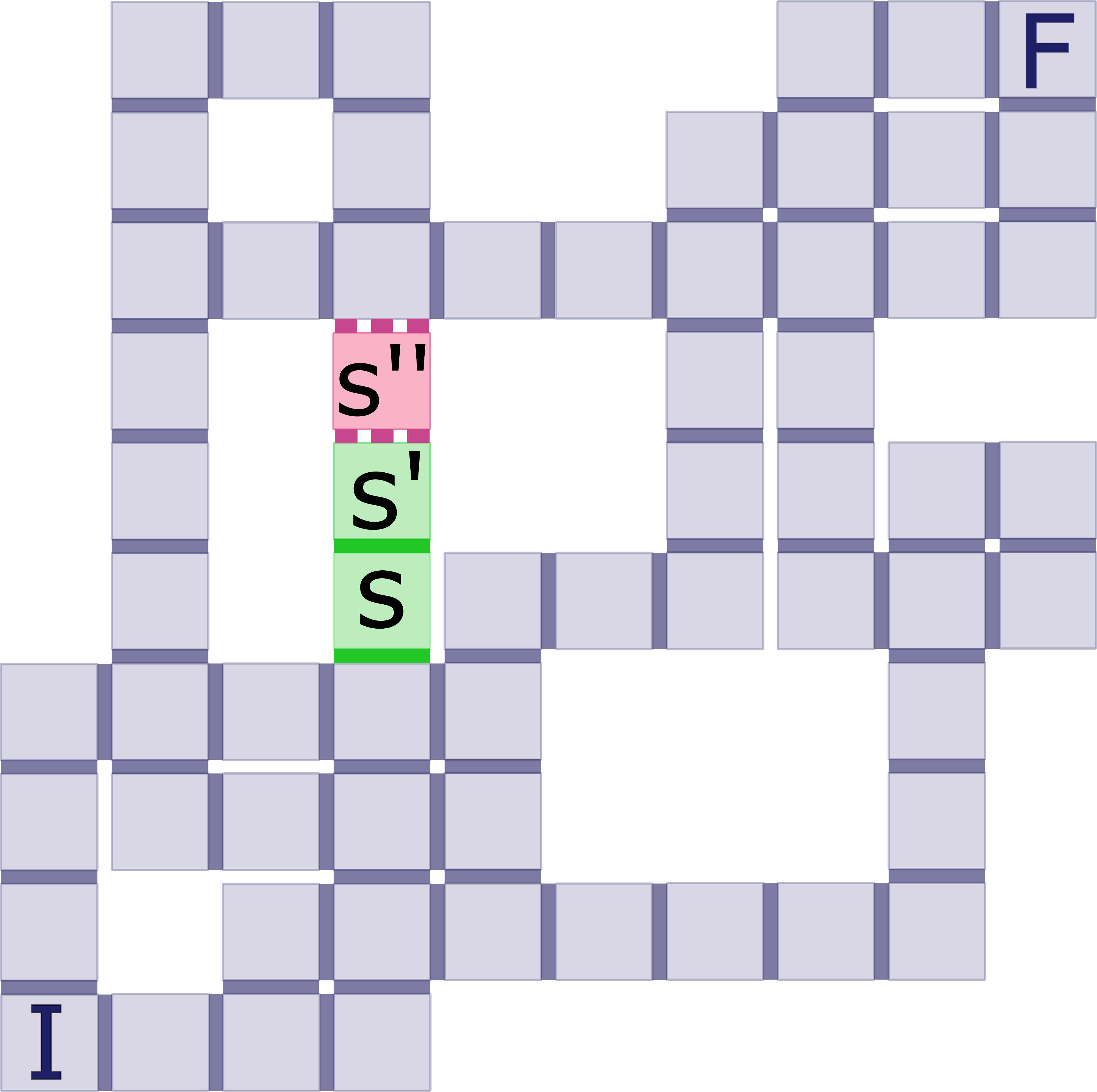
Figure 3: In the elaboration step, the simulation finds $s$ and $s^{\prime}$ but not $s^{\prime\prime}$. Without detailed balance, a slow transition from $s^{\prime}$ to $s$ could make the MFPT to $F$ large. However, in the full state space, $s^{\prime}$ might quickly reach $F$ via a fast transition to $s^{\prime\prime}$.

Therefore, for detailed-balance CTMCs, we elaborate the pathway to possibly include states that have a high probability of being visited with SSA but were not included with our biased sampling. Here, we use SSA to elaborate the pathway; we run $K$ simulations from each state of the pathway for a maximum simulation time of $\kappa$, meaning that a simulation stops as soon as the simulation time becomes greater than $\kappa$. By simulation time we mean the time of a SSA trajectory, not the wall-clock time. $K$ and $\kappa$ are tuning parameters that affect the quality of predictions. The running time of elaborating the states in the pathway with this approach is O($|\hat{\mathcal{S}}|K\kappa k_{\text{max}}$), where $\hat{\mathcal{S}}$ is the state space of the pathway and $k_{\text{max}}$ is the fastest rate in the pathway. Alternatively, we could use a fixed number of transitions instead of a fixed simulation time. Another approach is to add all states that are within distance $r$ of every state of the pathway. However, with this approach, the size of the state space could explode, whereas by using SSA the most probable states will be chosen.

Note that any elaboration which stops before hitting the target state might be problematic for non-detailed-balance CTMCs. Trajectories that stop while visiting a state for the first time might effectively be introducing a spurious sink into the enumerated state space. Without reversibility that last transition of the elaboration might be irreversible. Sink states that are not a target state make the MFPT to the target states infinite. For example in Figure 3, assume in the elaboration step, the simulation finds $s$ and $s^{\prime}$ but not $s^{\prime\prime}$ (or any other neighbor of $s^{\prime}$). Then without the reversible transition, $s^{\prime}$ will be a sink state and the MFPT to the target state $F$ will be infinite. Moreover, having reversible transitions that do not obey the detailed balance condition may make MFPT estimations large. For example, in Figure 3 assume that the reversible transitions between $s$ and $s^{\prime}$ do not obey detailed balance. Also, assume $\pi(s)$ and $\pi(s^{\prime})$ are both high, and that $\mathbf{K}(s,s^{\prime})$ is large whereas $\mathbf{K}(s^{\prime},s)$ is small. Therefore, if the elaboration stops at $s^{\prime}$ it will make the MFPT large. However, in the full state space, $s^{\prime}$ might quickly reach $F$ through a fast transition to $s^{\prime\prime}$. Thus, the state elaboration step may not be suitable for non-detailed-balance CTMCs.

Transition construction. After the previous two steps, fast transitions between the states of the pathway could still be missing. To make computations more accurate, we further compute all possible transitions in $\hat{\mathcal{S}}$ that were not identified in the previous two steps. In related roadmap planning work (Kavraki et al., 1996; Tang et al., 2005), states are connected to their nearest neighbors as identified by a distance metric. We can include all missing transitions by checking whether every two states in $\hat{\mathcal{S}}$ are neighbors in $\text{O}(|\hat{\mathcal{S}}|^{2})$ or by checking for every state in $\hat{\mathcal{S}}$ whether its neighbors are also in $\hat{\mathcal{S}}$ in O($|\hat{\mathcal{S}}|m\}$), where $m$ is the maximum number of neighbors of the states in the original CTMC.

$\delta$-pruning. Given a (truncated) CTMC in which we can compute the MFPT from every state to the target state, one question is: which states and transitions can be removed from the Markov chain without changing the MFPT from the initial states significantly? This question is especially relevant for the rapid evaluation of perturbed parameters, where MFPTs need to be recomputed often.

Given a CTMC $\mathcal{C}=(\mathcal{S},\mathbf{K},\mathbf{\pi}_{0},\mathcal{S}_{\mathrm{target}})$ and a pruning bound $\delta$, let the MFPT from any state $s$ to $\mathcal{S}_{\mathrm{target}}$ be $\tau_{s}$ and let the MFPT from the initial states to $\mathcal{S}_{\mathrm{target}}$ be $\tau_{\mathbf{\pi}_{0}}$. Let $\mathcal{S}_{\delta p}=\left\{s\in\mathcal{S}~{}\middle|~{}\tau_{s}<\delta\tau_{\mathbf{\pi}_{0}}\mbox{ and }\pi_{0}(s)=0\right\}$ be the set of states that are $\delta$-close to $\mathcal{S}_{\mathrm{target}}$ and that are not an initial state. We construct the $\delta$-pruned CTMC $\mathcal{C}_{\delta}=(\mathcal{S}_{\delta},\mathbf{\pi}_{0},\mathbf{K}_{\delta},\{s_{d}\})$ over the pruned set of states $\mathcal{S}_{\delta}=\mathcal{S}\setminus\mathcal{S}_{\delta p}\cup\left\{s_{d}\right\}$, where $s_{d}$ is the new target state. For $s,s^{\prime}\in\mathcal{S}_{\delta}\setminus\left\{s_{d}\right\}$, we update the rate matrix $\mathbf{K}_{\delta}:\mathcal{S}_{\delta}\rightarrow\mathbb{R}_{\geq 0}$ by $\mathbf{K}_{\delta}(s,s_{d})=\sum_{s^{\prime}\in\mathcal{S}_{\delta_{p}}}\mathbf{K}(s,s^{\prime})$ and $\mathbf{K}_{\delta}(s,s^{\prime})=\mathbf{K}(s,s^{\prime})$. Note that $\mathbf{K}_{\delta}(s_{d},s)$ is not used in the computation of the MFPT (Eq. 6), so we can simply assume $\mathbf{K}_{\delta}(s_{d},s)=0$. Alternatively, to retain detailed-balance conditions, we can define the energy of $s_{d}$ as $E(s_{d})=-RT\log\sum_{s^{\prime\prime}\in\mathcal{S}_{\delta p}}e^{-\frac{E(s^{\prime\prime})}{RT}}$ (see Eqs.7.1 and 7.2 from Schaeffer (Schaeffer, 2013)) and define $\mathbf{K}_{\delta}(s_{d},s)=e^{-\frac{E(s)-E(s_{d})}{RT}}\mathbf{K}_{\delta}(s,s_{d})$. For the pruned CTMC $\mathcal{C}_{\delta}=(\mathcal{S}_{\delta},\mathbf{\pi}_{0},\mathbf{K}_{\delta},\{s_{d}\})$, let the MFPT $\tau_{\mathbf{\pi}_{0}}^{\delta}$ be given as usual (Eq. 7). Then by construction

$$\tau_{\mathbf{\pi}_{0}}^{\delta}\leq\frac{\tau_{\mathbf{\pi}_{0}}}{1+\delta}.$$ (22)

We can calculate the MFPT from every state to the target states by solving Eq. 6 once for CTMC $\mathcal{C}$. Therefore, the running time of $\delta$-pruning depends on the running time of the matrix equation solver that is used. For a CTMC with state space $\mathcal{S}$, the running time of a direct solver is at most O($|\mathcal{S}|^{3}$). For iterative solvers the running time is generally less than O($|\mathcal{S}|^{3}$). After the equation is solved, the CTMC can be pruned in O($|\mathcal{S}|$) for any $\delta$. Note that for a given bound $\delta$, the running time for solving Eq. 6 for the pruned CTMC $\mathcal{C}_{\delta}$ might still be high. In that case, a larger value of $\delta$ is required. To set $\delta$ in practice, it could be useful to consider the number of states that will be pruned for a given $\delta$, that is $|\mathcal{S}_{\delta p}|$.

Updating perturbed parameters. We are interested in rapidly estimating the MFPT to target states given mildly perturbed parameters. Our approach is to reuse a truncated CTMC for mild perturbations. The MFPT estimates will be biased in this way. However, we could have significant savings in running time by avoiding the cost of sampling and building truncated CTMCs from scratch. We would still have to solve Eq. 6, but it could be negligible compared to the other costs. For example in Table 2, on average, solving the matrix equation is faster than SSA by a factor of 47 and is faster than building the truncated CTMC by a factor of 10.

A perturbed thermodynamic model parameter affects the energy of the states. Therefore, to update the transition rates, we would also have to recompute the energy of the states. A perturbed kinetic model only affects the transition rates. A perturbed experimental condition could affect both the energy of the states and the transition rates. Therefore, assuming the energy of a state can be updated in a constant time, the truncated CTMC can be updated in O($|\hat{\mathcal{S}}|+|\hat{\mathcal{E}}|$), where $\hat{\mathcal{E}}$ is the set of transitions of the truncated CTMC. For nucleic acid kinetics with elementary steps, the energy of a state can be computed from scratch in O($b$) time, or in O($1$) time using the energy calculations of a neighbor state (Schaeffer, 2013).

Quantifying the error. After we build truncated CTMCs, we need to quantify the error of MFPT estimates when experimental measurements are not available. It would help us set values for $N$, $\beta$, $K$ and $\kappa$ for fixed model parameters, and also evaluate when a truncated CTMC has a high error for perturbed model parameters. For exponential decay processes, one possible approach is to adapt the finite state projection FSP (Munsky and Khammash, 2006) method that is developed to quantify the error of truncated CTMCs for transient probabilities. We adapt it as follows. We combine all target states into one single absorbing state $s_{\text{f}}$. We project all states that are not in the truncated CTMC into an absorbing state $s_{o}$ and we redirect all transitions from the truncated CTMC to states out of the CTMC into $s_{o}$. Then we use the standard matrix exponential equations to compute the full distribution on the state space at a given time. However, we only care about the probabilities that $s_{\text{f}}$ and $s_{o}$ are occupied. We search to compute the half-completion time $t_{1/2}$ with bounds by

$$\begin{cases}t_{\text{min}}&\text{s.t. }p(s_{\text{f}}\;;\;t_{\text{min}})+p(s_{o}\;;\;t_{\text{min}})=\frac{1}{2},\\ t_{\text{max}}&\text{s.t. }p(s_{\text{f}}\;;\;t_{\text{max}})=\frac{1}{2},\end{cases}$$ (23)

where $p(s\;;\;t)$ is the probability that the process will be at state $s$ at time $t$ starting from the set of initial states. Since $s_{\text{f}}$ and $s_{o}$ are the only absorbing states, then $t_{\text{min}}$ exists and clearly $t_{\text{min}}\leq t_{1/2}$. Based on FSP, $p(s_{\text{f}}\;;\;t_{\text{max}})$ is an underestimate of the actual probability at time $t_{\text{max}}$, if it exists. A possible way to determine if a solutions exists is to determine the probability of reaching state $s_{\text{f}}$ compared to state $s_{o}$ from the initial states, which can be calculated by solving a system of linear equations (see Eq. 2.13 from Metzner, Schütte and Vanden-Eijnden (2009)). If the probability is greater or equal to $\frac{1}{2}$ then a solutions exists. If a solution does not exist for the given statespace, then based on FSP the error is guaranteed to decrease by adding more states and we can eventually find a solution to Eq. 23. The search for $t_{\text{max}}$ can be completed with binary search. Thus, the true $t_{1/2}$ is guaranteed to satisfy $t_{\text{min}}\leq t_{1/2}\leq t_{\text{max}}$. For exponential decay processes, the relation between the half-completion time and the MFPT is (Cohen-Tannoudji et al., 1977; Simmons, 1972)

$$t_{1/2}=\frac{\text{ln}2}{\lambda}\text{ and }\tau=\frac{1}{\lambda}\rightarrow\tau=\frac{t_{1/2}}{\text{ln}2},$$ (24)

where $\lambda$ is the rate of the process. Thus, $\frac{t_{\text{min}}}{\text{ln}2}\leq\tau\leq\frac{t_{\text{max}}}{\text{ln}2}$.

A drawback of this approach is that we might need a large number of states to find a solution to Eq. 23, which might make the master equation or the linear system solver infeasible in practice. Efficiently quantifying the error of MFPT estimates in truncated CTMCs for exponential and non-exponential decay processes is beyond the scope of this paper. It might be possible to use some other existing work (Kuntz et al., 2019; Backenköhler, Bortolussi and Wolf, 2019).

5 Dataset and Experiments for Interacting Nucleic Acid Strands

We implement pathway elaboration for interacting nucleic acid strands on top of Multistrand (Schaeffer, 2013; Schaeffer, Thachuk and Winfree, 2015) (see Section 3.1 for related background). Our framework and dataset are available at https://github.com/DNA-and-Natural-Algorithms-Group/PathwayElaboration.

Here, in Section 5.1, we describe our dataset of nucleic acid kinetics. In Section 5.2, we describe our experimental setup that is common in our experiments. In Section 5.3, we use pathway elaboration in a case study to gain insight on the kinetics of two contrasting reactions. In Section 5.4, first we evaluate estimations of pathway elaboration by comparing them with estimations of SSA. Then we build truncated CTMCs using SSA and TPS on a subset of our dataset and compare their performance with pathway elaboration. After that, we show the effectiveness of the $\delta$-pruning step. Finally, in Section 5.5, we use pathway elaboration for the rapid evaluation of perturbed parameters in parameter estimation.

5.1 Dataset of Interacting Nucleic Acid Strands

We conduct computational experiments on interacting nucleic acid strands (see Section 3.1 for related background). The speed at which nucleic acid strands interact is difficult to predict and depends on reaction topology, strands’ sequences, and experimental conditions. The number of secondary structures interacting nucleic strands may form is exponentially large in the length of the strands. Typical to these reactions are high energy barriers that prevent the reaction from completing, meaning that long periods of simulation time are required before successful reactions occur. Consider reactions that occur with rates lower than $10000\mbox{ M}^{-1}\mbox{ s}^{-1}$ such as three-way strand displacement at room temperature (see Table 1). These types of reactions are slow to simulate not because the simulator takes longer to generate trajectories for larger molecules, but the slowness is instead a result of the energy landscape: at low temperatures, duplexes simply are more stable, and require longer simulated time until their dissociation is observed. Predicting the kinetics of interacting nucleic acid strands is also difficult with classical machine learning methods and neural network models. For example, Zhang et al. (2018) successfully predict hybridization rates with a weighted neighbour voting prediction algorithm and Angenent-Mari et al. (2020) successfully predict toehold switch function with neural networks. However, despite the accurate and fast computational prediction of these methods, to treat different type of reactions or to treat different initial and target states the models have to be adapted. On the other hand, the CTMC model of Multistrand can readily be applied to unimolecular and bimolecular reactions. Moreover, the CTMC model could provide an unlimited number of unexpected intermediate states. In contrast, with the neural networks models of Angenent-Mari et al. (2020), which use attention maps to interpret intermediate states, the number is limited.

Table 1: Summary of the dataset of 267 nucleic acid kinetics. The initial concentration of the reactants is denoted as $u$ and $k$ is the experimental reaction rate constant.

Dataset No. Reaction type & source^† # of reactions Mean # of bases $[\text{Na}^{+}]$ (M) T (^∘C) u (M) $\mathop{\log_{10}}{k}$

2 Hairpin closing (Bonnet, Krichevsky and Libchaber, 1998) 62 25 0.15–0.5 10–49 ×110-8 3.2–4.8 3 Helix dissociation (Cisse, Kim and Ha, 2012) 39 18 0.01–0.2 23–37 ×110-8 -1.2–0.9 4 Helix association (Hata, Kitajima and Suyama, 2018) 43 46 0.195 25 ×510-8 4.0–6.7 5 Helix association (Zhang et al., 2018) 20 72 0.75 37–55 ×110-5 4.4–7.4 6 Toehold-mediated three-way strand displacement (Machinek et al., 2014) 10 102 0.05†† 23 ×510-9–×110-8 5.3–6.8 \begin{turn}{90.0}\mathcal{D}_{\text{train}}\end{turn}{\left\{\begin{tabular}[]{C{0.8cm}C{3.2cm} C{.9cm}C{0.8cm}C{1.4cm}C{0.9cm}C{1.2cm}C{1.2cm}}\hline\cr$1$\@add@centering&Hairpin opening~{}\cite[citep]{(\@@bibref{AuthorsPhrase1Year}{bonnet1998kinetics}{\@@citephrase{, }}{})}\@add@centering&$63$\@add@centering&$25$\@add@centering&$0.150.5$\@add@centering&$1049$\@add@centering&$1\times 10^{-8}$\@add@centering&$1.44.6$\@add@centering\\ \hline\cr$2$\@add@centering&Hairpin closing~{}\cite[citep]{(\@@bibref{AuthorsPhrase1Year}{bonnet1998kinetics}{\@@citephrase{, }}{})}\@add@centering&$62$\@add@centering&$25$\@add@centering&$0.150.5$\@add@centering&$1049$\@add@centering&$1\times 10^{-8}$\@add@centering&$3.24.8$\@add@centering\\ \hline\cr$3$\@add@centering&Helix dissociation~{}\cite[citep]{(\@@bibref{AuthorsPhrase1Year}{cisse2012rule}{\@@citephrase{, }}{})}\@add@centering&$39$\@add@centering&$18$\@add@centering&$0.010.2$\@add@centering&$2337$\@add@centering&$1\times 10^{-8}$\@add@centering&$-1.20.9$\@add@centering\\ \hline\cr$4$\@add@centering&Helix association~{}\cite[citep]{(\@@bibref{AuthorsPhrase1Year}{hata2017influence}{\@@citephrase{, }}{})}\@add@centering&$43$\@add@centering&$46$\@add@centering&$0.195$\@add@centering&$25$\@add@centering&$5\times 10^{-8}$\@add@centering&$4.06.7$\@add@centering\\ \hline\cr$5$\@add@centering&Helix association~{}\cite[citep]{(\@@bibref{AuthorsPhrase1Year}{zhang2018predicting}{\@@citephrase{, }}{})}\@add@centering&$20$\@add@centering&$72$\@add@centering&$0.75$\@add@centering&$3755$\@add@centering&$1\times 10^{-5}$\@add@centering&$4.47.4$\@add@centering\\ \hline\cr$6$\@add@centering&Toehold-mediated three-way strand displacement~{}\cite[citep]{(\@@bibref{AuthorsPhrase1Year}{machinek2014programmable}{\@@citephrase{, }}{})}\@add@centering&$10$\@add@centering&$102$\@add@centering&$0.05^{\dagger\dagger}$\@add@centering&$23$\@add@centering&$5\text{\times}{10}^{-9}1\text{\times}{10}^{-8}$\@add@centering&$5.36.8$\@add@centering\end{tabular}\right.}

1 Hairpin opening (Bonnet, Krichevsky and Libchaber, 1998) 63 25 0.15–0.5 10–49 ×110-8 1.4–4.6

$$\begin{turn}{90.0}\mathcal{D}_{\text{test}}\end{turn}{\left\{\begin{tabular}[]{C{0.8cm}C{3.2cm} C{.9cm}C{0.8cm}C{1.4cm}C{0.9cm}C{1.2cm}C{1.2cm}}\hline\cr$7$\@add@centering&Helix association~{}\cite[citep]{(\@@bibref{AuthorsPhrase1Year}{hata2017influence}{\@@citephrase{, }}{})}\@add@centering&$4$\@add@centering&$46$\@add@centering&$0.195$\@add@centering&$25$\@add@centering&$5\times 10^{-8}$\@add@centering&$4.05.0$\@add@centering\\ \hline\cr$8$\@add@centering&Toehold-mediated three-way strand displacement~{}\cite[citep]{(\@@bibref{AuthorsPhrase1Year}{machinek2014programmable}{\@@citephrase{, }}{})}\@add@centering&$26$\@add@centering&$100$\@add@centering&$0.05^{\dagger\dagger}$\@add@centering&23\@add@centering&$5\text{\times}{10}^{-9}1\text{\times}{10}^{-8}$\@add@centering&$2.76.3$\@add@centering\\ \hline\cr\end{tabular}\right.}$$

^† See Figure 2 for example figures of these reactions.
^†† The experiment was performed without $\text{Na}^{+}$ in the buffer.

We curate a dataset of 267 interacting DNA strands from the published literature, summarized in Table 1. The reactions are annotated with the temperature, the buffer condition, and the experimentally determined reaction rate constant. The dataset covers a wide range of slow and fast unimolecular and bimolecular reactions where the reaction rate constants vary over 8.6 orders of magnitude. For unimolecular reactions, we consider hairpin opening (Bonnet, Krichevsky and Libchaber, 1998), hairpin closing (Bonnet, Krichevsky and Libchaber, 1998), and helix dissociation (Cisse, Kim and Ha, 2012). For bimolecular reactions, we consider helix association (Hata, Kitajima and Suyama, 2018; Zhang et al., 2018) and toehold-mediated three-way strand displacement (Machinek et al., 2014). The reactions from Cisse, Kim and Ha (2012) and Machinek et al. (2014) may have mismatches between the bases of the strands. The type of reactions in Table 1 are widely used in nanotechnology, such as in molecular beacon probes (Chen et al., 2015).

For bimolecular reactions, we Boltzmann sample initial reacting complexes. For reactions in which we define only one target state, in the pathway construction step, we bias the paths towards that state. In this work, for reactions in which we define a set of target states, we bias paths towards only one target state, so that $\mathbf{\pi}^{\prime}(s_{b})=1$ for one state and $\mathbf{\pi}^{\prime}(s)=0$ for all other states. Next we describe these states.

Hairpin closing and hairpin opening. For a hairpin opening reaction, we define the initial state to be the system microstate in which a strand has fully formed a duplex and a loop (see Figure 2a). We define the target state to be the system microstate in which the strand has no base pairs. Hairpin closing is the reverse reaction, where a strand with no base pair forms a fully formed duplex and a loop.

Helix dissociation and helix association. For a helix dissociation reaction, we specify the initial state to be the system microstate in which two strands have fully formed a helix (see Figure 2b). We define the set of target states to be the set of system microstates in which the strands have detached and there are no base pairs within one of the strands. We bias paths towards the target state in which there are no base pairs formed within any of the strands. Helix association is the reverse reaction. We Boltzmann sample the initial reacting complexes in which the strands have not formed base pairs with each other. We define the target state to be the system microstate in which the duplex has fully formed.

Toehold-mediated three-way strand displacement. In this reaction, an invader strand displaces an incumbent strand in a duplex, where a toehold domain facilitates the reaction (see Figure 2c and Figure 4). We Boltzmann sample initial reacting complexes in which the incumbent and substrate form a complex through base pairing and the invader forms another complex. We define the set of target states to be the set of microstates where the incumbent is detached from the substrate and there are no base pairs within the incumbent. We bias paths towards the target state in which the substrate and invader have fully formed base pairs and there are no base pairs within the incumbent.

In datasets No. 1-6 from Table 1, we consider reactions that are feasible with SSA with our parameterization of Multistrand, given two weeks computation time, since we compare SSA results with pathway elaboration results. We indicate these reactions as $\mathcal{D}_{\text{train}}$ since we also use them as training set in Section 5.5. We indicate datasets No. 7-8 as $\mathcal{D}_{\text{test}}$ since we use them as testing set in Section 5.5.

5.2 Experimental Setup

Experiments are performed on a system with 64 2.13GHz Intel Xeon processors and 128GB RAM in total, running openSUSE Leap 15.1. An experiment for a reaction is conducted on one processor. Our framework is implemented in Python, on top of the Multistrand kinetic simulator (Schaeffer, 2013; Schaeffer, Thachuk and Winfree, 2015). To solve the matrix equations in Eq. 6, we use the sparse direct solver from SciPy (Virtanen et al., 2020) when possible. Otherwise we use the sparse iterative biconjugate gradient algorithm (Fletcher, 1976) from SciPy.

In all of our experiments, the thermodynamic parameters for predicting the energy of the states are fixed and the energies are calculated with Multistrand. Each reaction uses its own experimental condition as provided in the dataset. In all our experiments, we use the Metropolis kinetic model from Multistrand. For all experiments except for Section 5.5, we fix the kinetic parameters to the Metropolis Mode parameter set (Zolaktaf et al., 2017), that is $\theta_{1}=\{k_{\mathrm{uni}}\approx 2.41\times 10^{6}\text{ s}^{-1},k_{\mathrm{bi}}\approx 8.01\times 10^{5}\text{ M}^{-1}\text{s}^{-1}\}$. To obtain MFPTs with SSA, we use 1000 samples, except for three-way strand displacement reactions in which we use 100 samples, since the simulations take a longer time to complete.

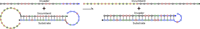
(a)

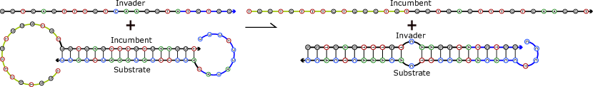
(b)

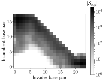
(c)

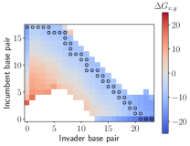
(d)

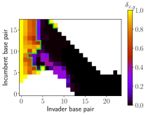
(e)

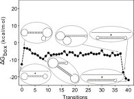
(f)

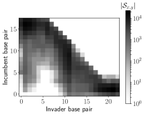
(g)

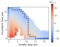
(h)

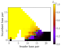
(i)

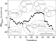
(j)

Figure 4: Results of truncated CTMCs built with pathway elaboration ($N=128$, $\beta=0.6$, $K=1024$, $\kappa=16$ ns) for two toehold-mediated three-way strand displacement reactions from Machinek et al. (2014). (a) A toehold-mediated three-way strand displacement reaction that has a 6-nt toehold and a 17-nt displacement domain (Machinek et al., 2014). (b) A toehold-mediated three-way strand displacement reaction that has a 6-nt toehold, a 17-nt displacement domain, and a mismatch exists between the invader and the substrate at position 6 of the displacement domain (Machinek et al., 2014). Figures 4c, 4d, 4e, and 4f correspond to Figure 4a. Figures 4g,4h,4i, and 4j correspond to Figure 4b. In Figures 4c, 4d, 4e, 4g, 4h, and 4i, the x-axis corresponds to the number of base pairs between the invader and the substrate, and the y-axis corresponds to the number of base pairs between the incumbent and the substrate. (c, g) At coordinate $(x,y)$, $|\mathcal{S}_{x,y}|$ is shown, where $\mathcal{S}_{x,y}$ is a system macrostate (a nonempty set of system microstates) equal to the set of states with coordinate $(x,y)$. (d, h) At coordinate $(x,y)$, the free energy $\Delta G_{x,y}$ is shown, which is defined as $\Delta G_{x,y}=-RT\ln\sum_{s\in\mathcal{S}_{x,y}}e^{\frac{-\Delta G(s)}{RT}}$ (Schaeffer, 2013). The free energy of the paths in Figures 4f and 4j are also shown with the $\circ$ marker in Figures 4d and 4h, respectively. (e, i) At coordinate $(x,y)$, the value of $\delta_{x,y}=\sum_{s\in\mathcal{S}_{x,y}}\frac{w_{s}\delta(s)}{\sum_{s\in\mathcal{S}_{x,y}}w_{s}}$ is shown, where $\delta(s)=\tau_{s}/\tau_{\mathbf{\pi}_{0}}$ and $w_{s}=e^{\frac{-\Delta G(s)}{RT}}$. For ease of understanding, the green “halfway line” separates coordinates where $\delta_{x,y}$ is greater than 0.5 from coordinates where $\delta_{x,y}$ is less than 0.5. (f, j) The free energy landscape of a random path built with pathway elaboration ($N=1$, $\beta=0$, $K=0$, $\kappa=0$ ns) and the initial and the final states and some states near the local extrema are illustrated.

5.3 Case Study

Here we illustrate the use of pathway elaboration to gain insight on the kinetics of two contrasting reactions from Machinek et al. (2014), one being a rare event.

Figures 4a and 4b show the two teohold-mediated three-way strand displacement reactions that we consider (Machinek et al., 2014). In the reaction in Figure 4a, the invader and substrate are complementary strands in the displacement domain. In the reaction in Figure 4b, there is a mismatch between the invader and the substrate in the displacement domain. The rate of toehold-mediated strand displacement is usually determined by the time to complete the first bimolecular transition, in which the invader forms a base pair with the substrate for the first time. However, the rate could be controlled by several orders of magnitude by altering positions across the strand, such as using mismatch bases (Machinek et al., 2014). The reaction in Figure 4b is approximately 3 orders of magnitude slower than the reaction in Figure 4a. For the reaction in Figure 4a, $\mathop{\log_{10}}k=6.43$, $\mathop{\log_{10}}\hat{k}_{\text{PE}}=6.62$, $\mathop{\log_{10}}\hat{k}_{\text{SSA}}=6.75$, $|\hat{\mathcal{S}}|=4.3\times 10^{5}$, the computation time of pathway elaboration is $1.4\times 10^{5}$ s, and the computation time of SSA is $3.9\times 10^{5}$ s. For the reaction in Figure 4b, $\mathop{\log_{10}}k=3.17$, $\mathop{\log_{10}}\hat{k}_{\text{PE}}=3.59$, $|\hat{\mathcal{S}}|=7\times 10^{5}$, the computation time of pathway elaboration is $2.7\times 10^{5}$ s, and SSA is not feasible within $1\times 10^{6}$ s.

In Figures 4c-4e and  4g-4i, we illustrate different properties of the truncated CTMCs for the reactions in Figures 4a and 4b, respectively. Comparing Figure 4c with Figure 4g, we see that many states are sampled midway in Figure 4g due to the mismatch. In Figures 4d and 4h, we compare the energy barrier (increase in free energy) while moving from the beginning of the x-axis towards the end of the x-axis. In Figure 4d, we can see a noticeable energy barrier in the beginning. However, in Figure 4h, we can see two noticeable energy barriers, one in the beginning and one midway. Figures 4e and 4i show states that are $\delta$-close to the target states. These figures show that with $\delta$-pruning, states that are further from the initial states and closer to the target states will be pruned with smaller values of $\delta$, compared to states that are closer to the initial states and further from the target states. Comparing Figure 4e with Figure 4i, the states quickly reach the target states after the first several transitions in Figure 4e (after the energy barrier). However, in Figure 4i, the states do not quickly reach the target states until after the second energy barrier. Figure 4f and 4j show the free energy landscape and some of the secondary structures for a random path from an initial state to a target state for the reactions in Figures 4a and 4b, respectively. For the reaction in Figure 4a, the barrier is near the first transition. For the reaction in Figure 4b, there is a noticeable barrier after several base pairs form between the invader and the substrate, presumably near the mismatch.

5.4 Mean First Passage Time and Reaction Rate Constant Estimation

To evaluate the estimations of pathway elaboration, we compare its estimations with estimations obtained from SSA for the reactions in $\mathcal{D}_{\text{train}}$. Note that for many of these reactions the size of the state space is exponentially large in the length of the strands. Therefore, exact matrix equations is not possible for them. Instead we use SSA since it can generate statistically correct trajectories. We also compare the wall-clock computation time of pathway elaboration with SSA.

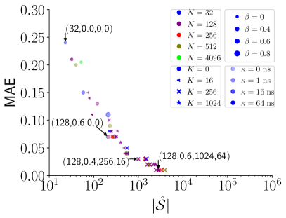
(a)

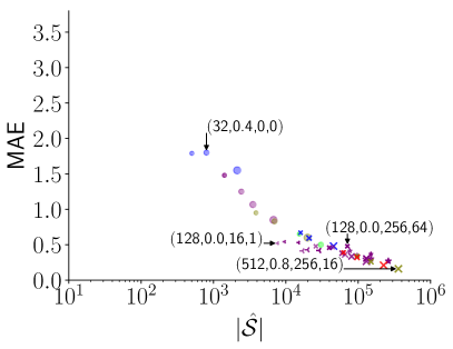
(b)

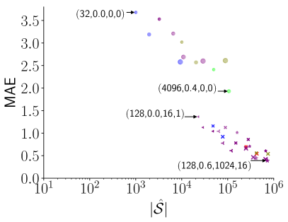
(c)

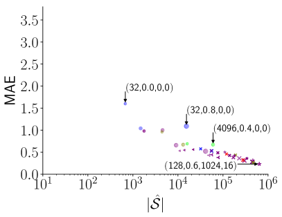
(d)

Figure 5: The MAE of pathway elaboration with SSA versus $|\hat{\mathcal{S}|}$ for different values of $N$, $\beta$, $K$ and $\kappa$. (a) datasets No. 1,2, and 3, (b) dataset No. 4, (c) dataset No. 5, and (d) dataset No. 6. The annotated values on the figures correspond to $N$, $\beta$, $K$, and $\kappa$, respectively.

We evaluate the estimations of pathway elaboration based on the mean absolute error (MAE) with SSA, which is defined over a dataset $\mathcal{D}$ as

$$\text{MAE}=\frac{1}{|\mathcal{D}|}\sum_{r\in\mathcal{D}}|\mathop{\log_{10}}\hat{\tau}_{\text{SSA}}^{r}-\mathop{\log_{10}}\hat{\tau}_{\text{PE}}^{r}|=\frac{1}{|\mathcal{D}|}\sum_{r\in\mathcal{D}}|\mathop{\log_{10}}\hat{k}_{\text{SSA}}^{r}-\mathop{\log_{10}}\hat{k}_{\text{PE}}^{r}|,$$ (25)

where $\hat{\tau}_{\text{PE}}^{r}$ and $\hat{\tau}_{\text{SSA}}^{r}$ are the estimated MFPTs of SSA and pathway elaboration for reaction $r$, respectively, and $\hat{k}_{\text{SSA}}^{r}$ and $\hat{k}_{\text{PE}}^{r}$ are the estimated reaction rate constants of SSA and pathway elaboration for reaction $r$, respectively. The equality follows from Eqs.  17 and 18. We use $\mathop{\log_{10}}$ differences since the reactions rate constants cover many orders of magnitude. We use the MAE as our evaluation metric since it is conceptually easy to understand. For example, here, an MAE of $1$ means on average the predictions are off by a factor of 10. In the rest of this subsection, we first look at the trade-off between the MAEs and the size of the truncated state space set $\hat{\mathcal{S}}$, with regards to different parameter settings of the pathway elaboration method. Then we look at the trade-off between the MAE and the computation time.

5.4.1 MAE of Pathway Elaboration with SSA versus $|\hat{\mathcal{S}}|$

Figure 5 shows the MAE of pathway elaboration with SSA versus $|\hat{\mathcal{S}}|$ of pathway elaboration for different configurations of the $N$, $\beta$, $K$, and $\kappa$ parameters. Figure A1p and A2 from the Appendix represent Figure 5 by varying only two parameters at a time. The figures show that generally as $N$ and $\beta$ increase, the MAE decreases. This is because for a fixed $N$ as $\beta\to 1$ the ensemble of paths will be generated by SSA. As $N\to\infty$, the truncated state space becomes larger and is more likely to contain the most probable paths from the initial states to the target states.

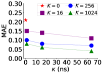
(a)

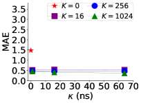
(b)

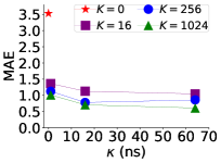
(c)

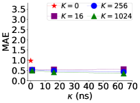
(d)

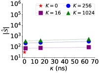
(e)

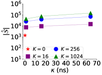
(f)

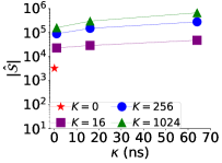
(g)

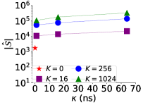
(h)

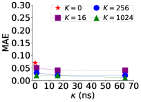
(i)

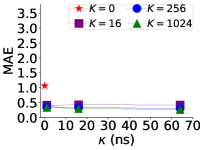
(j)

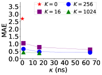
(k)

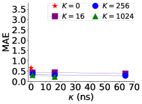
(l)

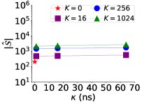
(m)

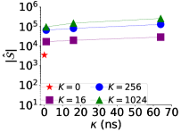
(n)

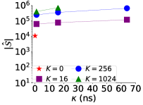
(o)

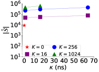
(p)

Figure A2: The effect of state elaboration, with different values of $K$ and $\kappa$ and fixed values of $N$ and $\beta$ on the MAE of pathway elaboration with SSA and the $|\hat{\mathcal{S}|}$ of pathway elaboration. $K=0$ indicates that the states of the pathway are not elaborated. In (a-h), $N=128$ and $\beta=0.0$ are fixed. In (i-p), $N=128$ and $\beta=0.6$ are fixed. (a), (e), (i), and (m) correspond to datasets No. 1,2, and 3. (b), (f), (j), and (n) correspond to dataset No. 4. (c) (g), (k), and (o) correspond to dataset No. 5. (d), (h), (l), and (p) correspond to dataset No. 6. For the missing settings, pathway elaboration did not finish within two weeks computation time.

Comparing the MAE of configurations where $K=0$ and $\kappa=0$ with other settings where $K>0$ and $\kappa>0$, shows that the elaboration step helps reduce the MAE (in the Appendix, compare Figures A1a-A1d with Figures A1i-A1l). Particularly, the elaboration step is useful for dataset No. 4, helix association from Zhang et al. (2018) where intra-strand base pairs can form before completing hybridization. The plots show that the elaboration step is more useful when $\beta$ is small (in the Appendix, compare Figures A2a-A2d with Figures A2i-A2l). This could be because elaboration helps find rate determining states that were not explored due to the biased sampling. When $\beta\to 1$ the pathway elaboration method will perform as SSA and rate determining states can be found without elaboration.

Furthermore, the figures show that as $K$ increases, the MAE decreases. However, with a large value for $\kappa$ and a small value of $K$ the performance could be diminished (such as in Figure A2c of the Appendix). In particular, consider that $K$ and $\kappa$ might involve simulations that go on excursions outside the ‘main’ densely-visited parts of the enumerated state space, and they might even terminate out there. Such excursions might very well introduce significant local minima into the enumerated state space - even when no significant local minima exist in the original full state space. For example, consider an excursion that goes off-path down a wide slope, perhaps toward the target state. If it terminates before reaching a target state, then a hypothetical simulation in the enumerated state space could get stuck, needing to climb back up the slope to the point where the excursion began. The expected hitting time in the enumerated state space will account for such wasted time, thus leading to an over estimation of the MFPT. Therefore, $\kappa$ should be tuned with respect to $K$.

Table 2: Pathway elaboration ($N=128$, $\beta=0.6$, $K=256$, $\kappa=16$ ns) versus SSA. The mean statistics are averaged over the ‘# of reactions’. Also, the pathway elaboration experiments are repeated three times and their mean is calculated. MAE refers to the mean absolute error of pathway elaboration with SSA (Eq. 25). $|\hat{\mathcal{S}}|$ is the size of the truncated state space. See Figure 6 for an illustration of individual reaction predictions.

Dataset No.	# of reactions	MAE	Mean $|\hat{\mathcal{S}}|$ for pathway elaboration	Mean matrix computation time (s) for pathway elaboration	Mean computation time (s) for pathway elaboration	Mean computation time (s) for SSA
$1$	$63$	$0.04$	$5.7\times 10^{2}$	$4.5\times 10^{-3}$	$1.0\times 10^{3}$	$2.7\times 10^{1}$
$2$	$62$	$0.03$	$1.8\times 10^{3}$	$1.5\times 10^{-2}$	$1.0\times 10^{3}$	$1.2\times 10^{1}$
$3$	$39$	$0.04$	$5.3\times 10^{2}$	$6.8\times 10^{-3}$	$1.6\times 10^{3}$	$3.8\times 10^{3}$
$4$	$43$	$0.29$	$8.1\times 10^{4}$	$3.0\times 10^{1}$	$2.1\times 10^{4}$	$4.9\times 10^{5}$
$5$	$20$	$0.51$	$3.8\times 10^{5}$	$2.3\times 10^{4}$	$1.6\times 10^{5}$	$3.7\times 10^{4}$
$6$	$10$	$0.31$	$3.0\times 10^{5}$	$1.3\times 10^{3}$	$1.3\times 10^{5}$	$3.8\times 10^{5}$
All datasets	$237$	$0.13$	$6.0\times 10^{4}$	$2.0\times 10^{3}$	$2.4\times 10^{4}$	$1.1\times 10^{5}$

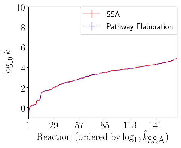
(a)

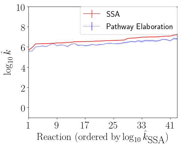
(b)

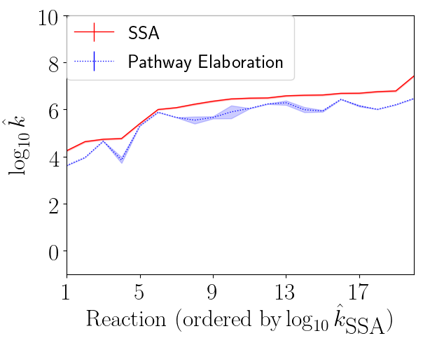
(c)

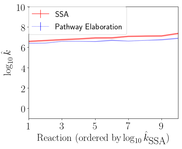
(d)

Figure 6: The $\mathop{\log_{10}}\hat{k}_{\text{SSA}}$ and $\mathop{\log_{10}}\hat{k}_{\text{PE}}$ ($N=128$, $\beta=0.6$, $K=256$, $\kappa=16\text{ ns}$) for (a) datasets No. 1,2, and 3, and (b) dataset No. 4, (c) dataset No. 5, and (d) dataset No. 6. The reactions are ordered along the x-axis by their predicted $\mathop{\log_{10}}\hat{k}_{\text{SSA}}$. The pathway elaboration experiments are repeated three times. For each reaction, $\mathop{\log_{10}}\hat{k}_{\text{PE}}$ is calculated by the average of the three experiments. The shaded area for pathway elaboration indicates the range (minimum to maximum) of the three experiments. The shaded area for SSA indicates the 95% percentile bootstrap of the $\mathop{\log_{10}}\hat{k}_{\text{SSA}}$.

5.4.2 MAE of Pathway Elaboration with SSA versus Computation Time

Table 2 illustrates the MAE and the computation time of pathway elaboration for when $N=128$, $\beta=0.6$, $K=256$, and $\kappa=16\text{ ns}$ compared with SSA. We illustrate this parameter setting because it provides a good trade-off between accuracy and computational time for the larger reactions. For the smaller reactions, we could achieve the same MAE with less computational time (by using smaller values for the parameter setting). Figure 6 further shows the prediction of pathway elaboration for this parameter setting compared to the prediction of SSA for individual reactions. In Table 2, the MAE for unimolecular reactions is smaller than $0.05$, whereas for bimolecular reactions it is larger than $0.29$. This is because the CTMCs for the bimolecular reactions in our dataset are naturally bigger than the CTMCs for the unimolecular reactions in our dataset, and require larger truncated CTMCs. The MAE can be further reduced by changing the parameters (as shown in Figure 5). With our implementation of pathway elaboration, the computation time of pathway elaboration for datasets No. 3, No. 4, and No. 6 are 2 times, 20 times, 3 times smaller than SSA, respectively. The computation time of SSA for datasets No. 1, No. 2, and No. 5 is smaller than the computation time of pathway elaboration. This is because pathway elaboration has some overhead, and in cases where SSA is already fast it can be slow. However, as we show in Section 5.5, even for these reactions, pathway elaboration could still be useful for the rapid evaluation of perturbed parameters. Also, the computation time for pathway elaboration could be significantly improved with more efficient implementations of the method.

5.4.3 Pathway Elaboration versus other Truncation-Based Approaches

Here we compare pathway elaboration with two other truncation-based approaches. (We do not compare with the probabilistic roadmap method, because we could not find a working implementation of this method, and because of the difficulty of determining appropriate transition rates between non-adjacent states as noted in our related work section.) The first truncated CTMC model that we include in our comparison uses SSA to sample paths from initial to target states, and builds a CTMC from these states. We call this method SSA-T, where the ”T” stands for truncated. Since the sampled paths from SSA are statistically correct, we want to see whether the estimate obtained by pathway elaboration compares well with the unbiased SSA-T estimates. We compare SSA-T with pathway elaboration only on our first two datasets, since SSA-T, being unsuitable for rare events, is too slow to run on our other datasets with the implementation that we used. Our second truncated CTMC model uses transition path sampling, and so we call it TPS-T. Our implementation of TPS-T first generates a single path that connects the initial and target states, using SSA. Then a new path is generated by choosing a random state in the most recently generated path, and finding a path from this randomly-chosen state. If the simulated path reaches the initial state before reaching a target state, we continue the simulation until a target state is reached. Moreover, we could define the simulations for TPS-T to be time-limited and include states from these simulations in the truncated CTMC. However, in our experiments stopping simulations early generally result in higher MAE compared to continuing simulations until target states are reached. In our experiments, we generate 128 paths in total for both SSA-T and TSP-T. As in Table 2, for pathway elaboration, we use $N=128$, $\beta=0.6$, $K=256$, and $\kappa=16\text{ ns}$.

Table 3 compares the MAE and computation time of CTMCs that are built with pathway elaboration versus CTMCs that are built with SSA and TPS. Figure 7 further shows the prediction of these methods compared for individual reactions. Datasets No. 1 and 2 are used in this table which are hairpin opening and closing, respectively. The MAE of pathway elaboration with SSA ($0.04$ and $0.03$) compares well with the MAE of SSA-T with SSA ($0.03$ and $0.03$). However, the MAE and the variance of TPS-T is high because the paths are correlated and depend on the initial path (Singhal, Snow and Pande, 2004). Increasing the number of simulations would reduce the variance of the predictions.

For a comparison of these methods with pathway elaboration regarding computation time, we have adapted our code for pathway elaboration to implement these methods. In our experiments, the computation time of pathway elaboration is smaller than both SSA-T and TPS-T and the computation time of TPS-T is smaller than the computation time of SSA-T.

Table 3: Building truncated CTMCs with pathway elaboration versus building truncated CTMCs with SSA (which we call SSA-T) and TPS (which we call TPS-T). For pathway elaboration, $N=128$, $\beta=0.6$, $K=256$, and $\kappa=16\text{ ns}$. For SSA-T and TPS-T, 128 successful simulations are used. The mean statistics are averaged over the ‘# of reactions’. Also, the experiments for each truncation-based approach is repeated three times and their mean is calculated. MAE refers to the mean absolute error of a method with SSA. $|\hat{\mathcal{S}}|$ is the size of the truncated state space. The mean matrix computation time for all methods is less than 0.1 (s). See Figure 7 for an illustration of individual reaction predictions.

Dataset No.	# of reactions	Method	MAE	Mean $|\hat{\mathcal{S}}|$	Mean computation time (s)
1	63	Pathway elaboration	$0.04$	$5.7\times 10^{2}$	$1.0\times 10^{3}$
		SSA-T	$0.03$	$4.0\times 10^{2}$	$1.4\times 10^{5}$
		TPS-T	$0.18$	$1.6\times 10^{2}$	$2.0\times 10^{4}$
2	62	Pathway elaboration	$0.03$	$1.8\times 10^{3}$	$1.0\times 10^{3}$
		SSA-T	$0.03$	$1.7\times 10^{3}$	$1.3\times 10^{4}$
		TPS-T	$0.34$	$3.2\times 10^{2}$	$1.7\times 10^{3}$

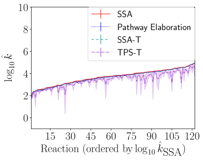
Figure 7: The $\mathop{\log_{10}}\hat{k}$ of SSA, pathway elaboration, SSA-T, and TPS-T for datasets No. 1 and 2. The reactions are ordered along the x-axis by their predicted $\mathop{\log_{10}}\hat{k}_{\text{SSA}}$. The experiments for each truncation-based approach is repeated three times, where for each reaction, $\mathop{\log_{10}}\hat{k}$ is calculated by the average of the three experiments. The shaded area for each truncation-based approach indicates the range (minimum to maximum) of its three experiments. The shaded area for SSA indicates the 95% percentile bootstrap of the $\mathop{\log_{10}}\hat{k}_{\text{SSA}}$. See Table 3 for parameter settings and mean statistics.

5.4.4 $\delta$-Pruning

Figure 8 shows how $\delta$-pruning affects the quality of the $\mathop{\log_{10}}$ reaction rate constant estimates, the size of the state spaces, and the computation time of solving the matrix equations, for dataset No. 6. The MFPT estimates satisfy the bound given by Eq. 22 whilst $\delta$-pruning reduces the computation time for solving the matrix equations by an order of magnitude for $\delta=0.6$. Using larger values of $\delta$ we can further decrease the computation time. If we reuse the CTMCs many times, such as in parameter estimation, $\delta$-pruning could help reduce computation time significantly.

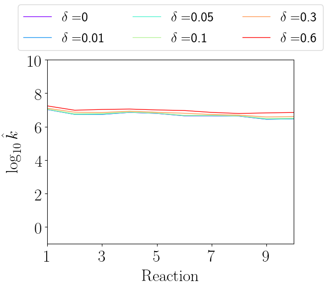
(a)

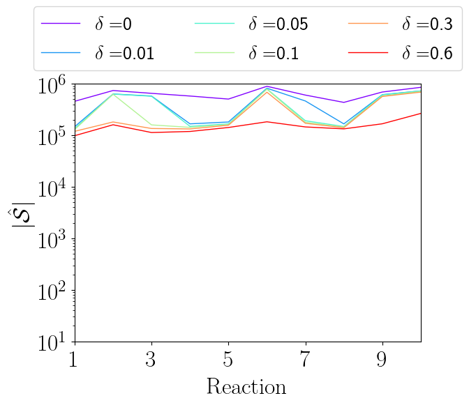
(b)

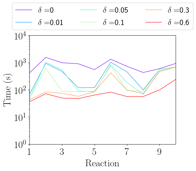
(c)

Figure 8: The effect of $\delta$-pruning with different values of $\delta$ on truncated CTMCs that are built with pathway elaboration ($N=128$, $\beta=0.6$, $K=1024$, $\kappa=16\text{ ns}$) for dataset No. 6. $\delta=0$ indicates $\delta$-pruning is not used. (a) The $\mathop{\log_{10}}\hat{k}$. (b) The size of the truncated state space $|\hat{\mathcal{S}}|$. (c) The computation time for solving Eq. 6.

5.5 Parameter Estimation

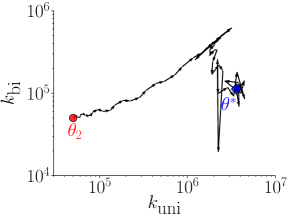
(a)

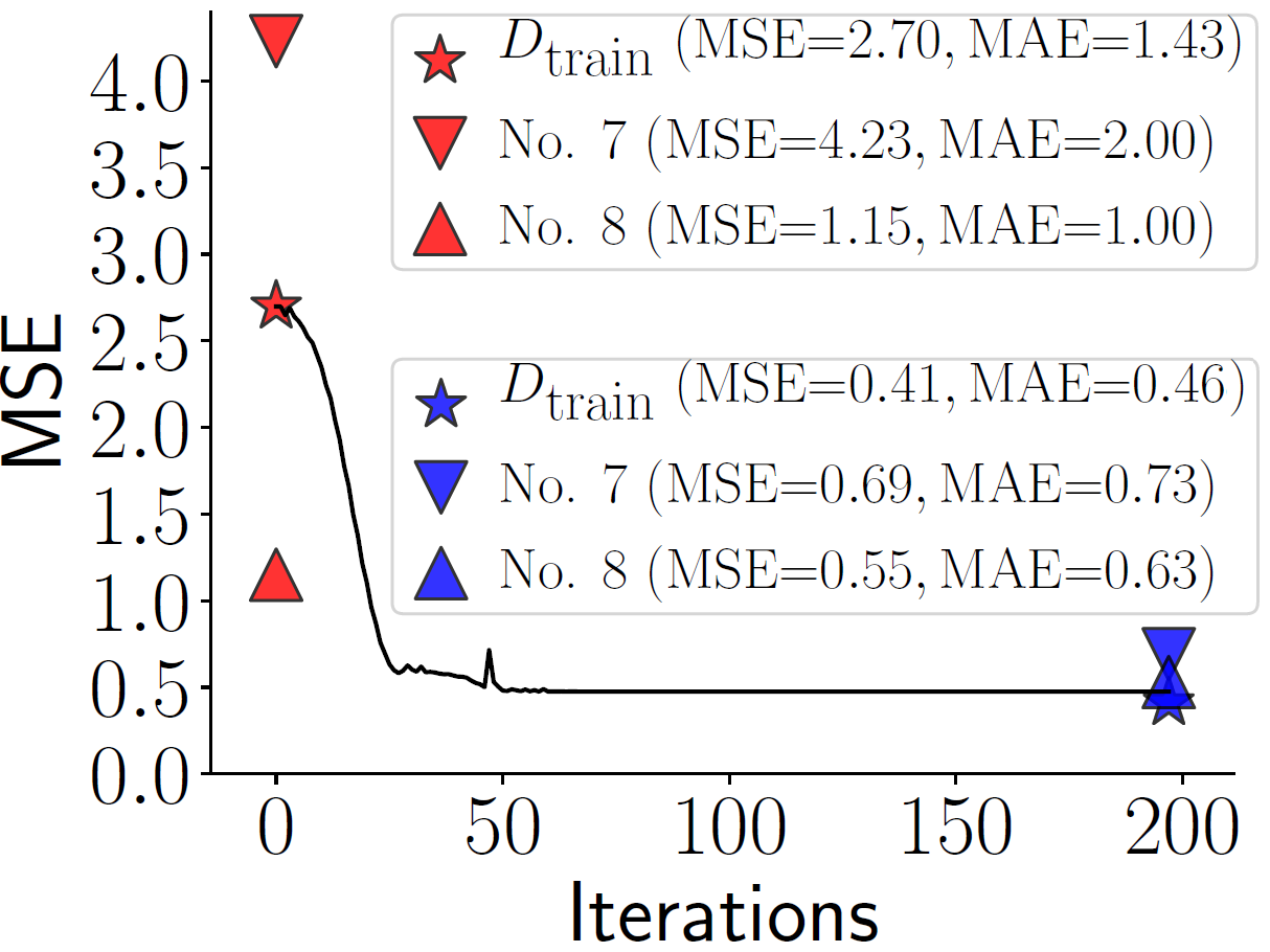
(b)

Figure 9: Results of parameter estimation using pathway elaboration ($N=128$, $\beta=0.4$, $K=256$, $\kappa=16\text{ ns}$). (a) The parameters are optimized from an initial simplex of $\theta_{2}$ and its perturbations to $\theta^{*}=\{k_{\mathrm{uni}}\approx 3.61\times 10^{6}\text{ s}^{-1},k_{\mathrm{bi}}\approx 1.12\times 10^{5}\text{ M}^{-1}\text{ s}^{-1}\}$. (b) The parameters are optimized using $\mathcal{D}_{\text{train}}$, shown with a line graph, and evaluated on dataset No. 7 and No. 8. The markers are annotated with the MSE and MAE of the datasets when the truncated CTMCs are built from scratch using $\theta_{2}$ and $\theta^{*}$.

In the previous subsections the underlying parameters of the CTMCs were fixed. Here we assume the parameters of the kinetic model of the CTMCs are not calibrated and we use pathway elaboration to build truncated CTMCs to rapidly evaluate perturbed parameter sets during parameter estimation. We use the 237 reactions indicated as $\mathcal{D}_{\text{train}}$ in Table 1 as our training set. We use the 30 rare event reactions indicated as $\mathcal{D}_{\text{test}}$ in Table 1 to show that given a well-calibrated parameter set for the CTMC model, the pathway elaboration method can estimate MFPTs and reaction rate constants of reactions close to their experimental measurement.

We seek the parameter set that minimizes the mean squared error (MSE) as

$$\begin{split}&\theta^{*}=\underset{\theta}{\text{argmin }}\frac{1}{|\mathcal{D}_{\text{train}}|}\sum_{r\in\mathcal{D}_{\text{train}}}{(\mathop{\log_{10}}\tau^{r}-\mathop{\log_{10}}\hat{\tau}_{\text{PE}}^{r}(\theta))^{2}}=\\ &\underset{\theta}{\text{argmin }}\frac{1}{|\mathcal{D}_{\text{train}}|}\sum_{r\in\mathcal{D}_{\text{train}}}{(\mathop{\log_{10}}k^{r}-\mathop{\log_{10}}\hat{k}_{\text{PE}}^{r}(\theta))^{2}},\end{split}$$ (26)

which is a common cost function for regression problems. The equality follows from Eqs.  17 and 18. We use the Nelder-Mead optimization algorithm (Nelder and Mead, 1965; Virtanen et al., 2020) to minimize the MSE. We initialize the simplex in the algorithm with $\theta_{2}=\{k_{\mathrm{uni}}=5\times 10^{4}\text{ s}^{-1},k_{\mathrm{bi}}=5\times 10^{4}\text{ M}^{-1}\text{s}^{-1}\}$ in which we choose arbitrarily and two perturbed parameter sets. Each perturbed parameter set is obtained from $\theta_{2}$ by multiplying one of the parameters by $1.05$, which is the default implementation of the optimization software (Virtanen et al., 2020). For every reaction, we also initialize the Multistrand kinetic model with $\theta_{2}$. We build truncated CTMCs with pathway elaboration ($N=128$, $\beta=0.4$, $K=256$, $\kappa=16\text{ ns}$). Whenever the matrix equation solving time is large (here we consider a time of $120$ s large), we use $\delta$-pruning (here we use $\delta$ values of $0.01-0.6$) to reduce the time. During the optimization, for a new parameter set we update the parameters in the kinetic model of the truncated CTMCs and we reuse the truncated CTMC to evaluate the parameter set. Similar to our previous work (Zolaktaf et al., 2019), to reduce the bias and to ensure that the truncated CTMCs are fair with respect to the optimized parameters, we can occasionally rebuild truncated CTMCs from scratch.

Although we use the MSE of pathway elaboration with experimental measurements as our cost function in the optimization procedure, the MAE of pathway elaboration with experimental measurements also decreases. Figure 9 shows how the parameters, the MSE, and the MAE change during optimization. The markers are annotated with the MSE and the MAE of $\mathcal{D}_{\text{train}}$ and datasets No. 7-8 when truncated CTMCs are built from scratch. The MAE of $\mathcal{D}_{\text{train}}$ with the initial parameter set $\theta_{2}$ is $1.43$. The optimization finds $\theta^{*}=\{k_{\mathrm{uni}}\approx 3.61\times 10^{6}\text{ s}^{-1},k_{\mathrm{bi}}\approx 1.12\times 10^{5}\text{ M}^{-1}\text{ s}^{-1}\}$ and reduces the MAE of $\mathcal{D}_{\text{train}}$ to $0.46$. The MAE of dataset No. 7 and dataset No. 8, which are not used in the optimization, reduce from $2.00$ to $0.73$ and from $1.00$ to $0.63$, respectively.

Overall, the experiment in this subsection shows that pathway elaboration enables MFPT estimation of rare events. It predicts their MFPTs close to their experimental measurements given an accurately calibrated model for their CTMCs. Moreover, it shows that pathway elaboration enables the rapid evaluation of perturbed parameters and makes feasible tasks such as parameter estimation which benefit from such methods. On average for the 30 reactions in the testing set, pathway elaboration takes less than two days, whereas SSA is not feasible within two weeks. The entire experiment in Figure 9 takes less than five days parallelized on 40 processors. Note that clearly our optimization procedure could be improved, for example by using a larger dataset or a more flexible kinetic model. However, this experiment is a preliminary study; we leave a rigorous study on calibrating nucleic acid kinetic models with pathway elaboration and possible improvements to future studies.

6 Discussion

Motivated by the problem of predicting nucleic acid kinetics, we address the problem of estimating MFPTs of rare events in large CTMCs and also the rapid evaluation of perturbed parameters. We propose the pathway elaboration method, which is a time-efficient probabilistic truncation-based approach for MFPT estimation in CTMCs. We conduct computational experiments on a wide range of experimental measurements to show pathway elaboration is suitable for predicting nucleic acid kinetics. In summary, our results are promising, but there is still room for improvement.

Using pathway elaboration, in the best possible case, the sampled region of states and transitions is obtained faster than SSA, but without significant bias in the collected states and transitions. The sampled region may however qualitatively differ from what would be obtained from SSA, which may compromise the MFPT estimates. Moreover, reusing truncated CTMCs for significantly perturbed parameters could lead to inaccurate estimation of the MFPT in the original CTMC. In Section 4, for exponential decay processes, we introduced a method that could help us quantify the error of the MFPT estimate. However, it might be slow in practice. So how can we efficiently tune these parameters? Similar to SSA, for a fixed $\beta$ and when $K=0$ and $\kappa=0$, we could increase $N$ until the estimated MFPT stops changing significantly (based on the law of large numbers it will converge). Note that for $K=0$ and $\kappa=0$ we could compute the MFPT by computing the average of the biased paths without solving matrix equations. As shown in Proposition 4.1, if we set $\beta$ to less than $1/2$, then biased paths will reach target states in expected time that is linear in the distance from initial to target states. For setting $K$, one possibility is to consider the number of neighbors of each state. A reaction where states have a lot of neighbors requires a larger $K$ compared to a reaction where states have a smaller number of neighbors. $\kappa$ should be set with respect to $K$. As stated in Section 5, a large value of $\kappa$ along with a small value of $K$ could result in excursions that do not reach any target state and lead to overestimates of the MFPT. One could set $\kappa$ to a small value and then increase $K$ until the MFPT estimate stops changing, and could repeat this process while feasible.

In the pathway elaboration method, we estimate MFPTs by solving matrix equations. Thus, its performance depends on the accuracy and speed of matrix equation solvers. For example, applying matrix equation solvers may not be suitable if the initial states lie very far from the target states, since the size of the truncated CTMCs depends on the shortest-path distance between these states. Although solving matrix equations through direct and iterative methods has progressed, both theoretically and practically (Fletcher, 1976; Virtanen et al., 2020; Cohen et al., 2018), solving stiff (multiple time scales) or very large equations could still be problematic in practice. More stable and faster solvers would allow us to estimate MFPTs for stiffer and larger truncated CTMCs. Moreover, it might be possible to use fast updates for solving the matrix equations (Brand, 2006; Parks et al., 2006). Therefore, if we require to compute MFPT estimates with matrix equations as we monotonically grow the size of the state space or for a perturbed parameter set, the total cost for solving all the linear systems would be the same cost as solving the final linear system from scratch.

We might be able to improve the pathway elaboration method to relieve the limitations discussed above. For example, it might be possible to use an ensemble of truncated CTMCs to obtain an unbiased estimate of the MFPT (Georgoulas, Hillston and Sanguinetti, 2017). To avoid excursions that lead to overestimation of the MFPT in the state elaboration step, we could run the pathway construction step from the last states visited in the state elaboration step. This would also relax the constraint of having reversible or detailed balance transitions. Presumably, an alternating approach of the two steps would make the approach more flexible. Moreover, currently we run the state elaboration step from every state of the pathway with the same setting. Efficiently running the state elaboration step as necessary, could reduce the time to construct the truncated CTMC in addition to the matrix computation time.

Finally, we evaluated the pathway elaboration method for predicting the MFPT of nucleic acid kinetics. However, the method is generally applicable to detailed-balance CTMC models, such as chemical reaction networks (Anderson and Kurtz, 2011) and protein folding (McGibbon and Pande, 2015).

Appendix A Appendix: The Mean Absolute Error of the Pathway Elaboration Method for Nucleic Acid Kinetics

Figures A1p and A2 represent Figure 5 by varying only two parameters at a time.

  In (a-h), $K=0$ and $\kappa=0$ ns are fixed (the state elaboration step is not used).

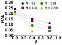
(a)

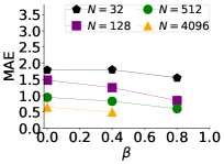
(b)

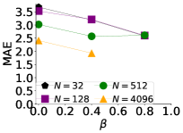
(c)

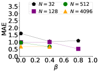
(d)

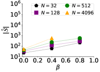
(e)

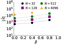
(f)

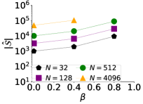
(g)

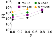
(h)

   In (a-h), $K=256$ and $\kappa=16\text{ ns}$ are fixed.

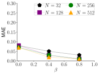
(i)

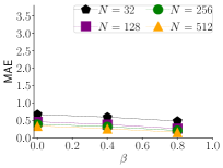
(j)

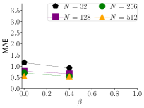
(k)

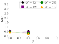
(l)

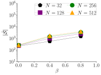
(m)

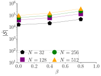
(n)

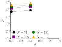
(o)

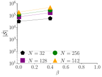
(p)

Figure A1: The effect of pathway construction with different values of $N$ and $\beta$ and fixed values of $K$ and $\kappa$ on the MAE of pathway elaboration with SSA and the $|\hat{\mathcal{S}|}$ of pathway elaboration. In (a-h), $K=0$ and $\kappa=0\text{ ns}$ are fixed. $K=0$ indicates that the states of the pathway are not elaborated. In (i-p), $K=256$ and $\kappa=16\text{ ns}$ are fixed. (a), (e), (i), and (m) correspond to datasets No. 1,2, and 3. (b), (f), (j), and (n) correspond to dataset No. 4. (c) (g), (k), and (o) correspond to dataset No. 5. (d), (h), (l), and (p) correspond to dataset No. 6. For the missing settings, pathway elaboration did not finish within two weeks computation time.

 

                                 In (a-h), $N=128$ and $\beta=0.0$ are fixed.                                              
   
        In (i-p), $N=128$ and $\beta=0.6$ are fixed.

References

- Allen, Valeriani and ten Wolde (2009) {barticle}[author] \bauthor\bsnmAllen, \bfnmRosalind J\binitsR. J., \bauthor\bsnmValeriani, \bfnmChantal\binitsC. and \bauthor\bparticleten \bsnmWolde, \bfnmPieter Rein\binitsP. R. (\byear2009). \btitleForward flux sampling for rare event simulations. \bjournalJournal of Physics: Condensed Matter \bvolume21 \bpages463102. \endbibitem
- Anderson and Kurtz (2011) {bincollection}[author] \bauthor\bsnmAnderson, \bfnmDavid F\binitsD. F. and \bauthor\bsnmKurtz, \bfnmThomas G\binitsT. G. (\byear2011). \btitleContinuous time Markov chain models for chemical reaction networks. In \bbooktitleDesign and Analysis of Biomolecular Circuits \bpages3–42. \bpublisherSpringer. \endbibitem
- Andrieu et al. (2003) {barticle}[author] \bauthor\bsnmAndrieu, \bfnmChristophe\binitsC., \bauthor\bsnmDe Freitas, \bfnmNando\binitsN., \bauthor\bsnmDoucet, \bfnmArnaud\binitsA. and \bauthor\bsnmJordan, \bfnmMichael I\binitsM. I. (\byear2003). \btitleAn introduction to MCMC for machine learning. \bjournalMachine learning \bvolume50 \bpages5–43. \endbibitem
- Angenent-Mari et al. (2020) {barticle}[author] \bauthor\bsnmAngenent-Mari, \bfnmNicolaas M\binitsN. M., \bauthor\bsnmGarruss, \bfnmAlexander S\binitsA. S., \bauthor\bsnmSoenksen, \bfnmLuis R\binitsL. R., \bauthor\bsnmChurch, \bfnmGeorge\binitsG. and \bauthor\bsnmCollins, \bfnmJames J\binitsJ. J. (\byear2020). \btitleA deep learning approach to programmable RNA switches. \bjournalNature Communications \bvolume11 \bpages1–12. \endbibitem
- Asmussen and Glynn (2007) {bbook}[author] \bauthor\bsnmAsmussen, \bfnmSøren\binitsS. and \bauthor\bsnmGlynn, \bfnmPeter W\binitsP. W. (\byear2007). \btitleStochastic simulation: algorithms and analysis \bvolume57. \bpublisherSpringer Science & Business Media. \endbibitem
- Azimzadeh and Forsyth (2016) {barticle}[author] \bauthor\bsnmAzimzadeh, \bfnmParsiad\binitsP. and \bauthor\bsnmForsyth, \bfnmPeter A\binitsP. A. (\byear2016). \btitleWeakly chained matrices, policy iteration, and impulse control. \bjournalSIAM Journal on Numerical Analysis \bvolume54 \bpages1341–1364. \endbibitem
- Backenköhler, Bortolussi and Wolf (2019) {barticle}[author] \bauthor\bsnmBackenköhler, \bfnmMichael\binitsM., \bauthor\bsnmBortolussi, \bfnmLuca\binitsL. and \bauthor\bsnmWolf, \bfnmVerena\binitsV. (\byear2019). \btitleBounding Mean First Passage Times in Population Continuous-Time Markov Chains. \bjournalarXiv preprint arXiv:1910.12562. \endbibitem
- Bolhuis et al. (2002) {barticle}[author] \bauthor\bsnmBolhuis, \bfnmPeter G\binitsP. G., \bauthor\bsnmChandler, \bfnmDavid\binitsD., \bauthor\bsnmDellago, \bfnmChristoph\binitsC. and \bauthor\bsnmGeissler, \bfnmPhillip L\binitsP. L. (\byear2002). \btitleTransition path sampling: Throwing ropes over rough mountain passes, in the dark. \bjournalAnnual Review of Physical Chemistry \bvolume53 \bpages291–318. \endbibitem
- Bonnet, Krichevsky and Libchaber (1998) {barticle}[author] \bauthor\bsnmBonnet, \bfnmGrégoire\binitsG., \bauthor\bsnmKrichevsky, \bfnmOleg\binitsO. and \bauthor\bsnmLibchaber, \bfnmAlbert\binitsA. (\byear1998). \btitleKinetics of conformational fluctuations in DNA hairpin-loops. \bjournalProceedings of the National Academy of Sciences \bvolume95 \bpages8602–8606. \endbibitem
- Brand (2006) {barticle}[author] \bauthor\bsnmBrand, \bfnmMatthew\binitsM. (\byear2006). \btitleFast low-rank modifications of the thin singular value decomposition. \bjournalLinear Algebra and its Applications \bvolume415 \bpages20–30. \endbibitem
- Cao, Gillespie and Petzold (2007) {barticle}[author] \bauthor\bsnmCao, \bfnmYang\binitsY., \bauthor\bsnmGillespie, \bfnmDaniel T\binitsD. T. and \bauthor\bsnmPetzold, \bfnmLinda R\binitsL. R. (\byear2007). \btitleAdaptive explicit-implicit tau-leaping method with automatic tau selection. \bjournalThe Journal of Chemical Physics \bvolume126 \bpages224101. \endbibitem
- Chen et al. (2015) {barticle}[author] \bauthor\bsnmChen, \bfnmYuan-Jyue\binitsY.-J., \bauthor\bsnmGroves, \bfnmBenjamin\binitsB., \bauthor\bsnmMuscat, \bfnmRichard A\binitsR. A. and \bauthor\bsnmSeelig, \bfnmGeorg\binitsG. (\byear2015). \btitleDNA nanotechnology from the test tube to the cell. \bjournalNature nanotechnology \bvolume10 \bpages748–760. \endbibitem
- Cisse, Kim and Ha (2012) {barticle}[author] \bauthor\bsnmCisse, \bfnmIbrahim I\binitsI. I., \bauthor\bsnmKim, \bfnmHajin\binitsH. and \bauthor\bsnmHa, \bfnmTaekjip\binitsT. (\byear2012). \btitleA rule of seven in Watson-Crick base-pairing of mismatched sequences. \bjournalNature Structural & Moleuclar Biology \bvolume19 \bpages623. \endbibitem
- Cohen et al. (2018) {binproceedings}[author] \bauthor\bsnmCohen, \bfnmMichael B\binitsM. B., \bauthor\bsnmKelner, \bfnmJonathan\binitsJ., \bauthor\bsnmKyng, \bfnmRasmus\binitsR., \bauthor\bsnmPeebles, \bfnmJohn\binitsJ., \bauthor\bsnmPeng, \bfnmRichard\binitsR., \bauthor\bsnmRao, \bfnmAnup B\binitsA. B. and \bauthor\bsnmSidford, \bfnmAaron\binitsA. (\byear2018). \btitleSolving directed laplacian systems in nearly-linear time through sparse LU factorizations. In \bbooktitle2018 IEEE 59th Annual Symposium on Foundations of Computer Science (FOCS) \bpages898–909. \bpublisherIEEE. \endbibitem
- Cohen-Tannoudji et al. (1977) {bbook}[author] \bauthor\bsnmCohen-Tannoudji, \bfnmClaude\binitsC., \bauthor\bsnmDavies, \bfnmPaul CW\binitsP. C., \bauthor\bsnmDiu, \bfnmBernard\binitsB., \bauthor\bsnmLaloe, \bfnmFranck\binitsF., \bauthor\bsnmDui, \bfnmBernard\binitsB. \betalet al. (\byear1977). \btitleQuantum mechanics \bvolume1. \bpublisherJohn Wiley & Sons. \endbibitem
- Dinh and Sidje (2016) {barticle}[author] \bauthor\bsnmDinh, \bfnmKhanh N\binitsK. N. and \bauthor\bsnmSidje, \bfnmRoger B\binitsR. B. (\byear2016). \btitleUnderstanding the finite state projection and related methods for solving the chemical master equation. \bjournalPhysical Biology \bvolume13 \bpages035003. \endbibitem
- Dinh and Sidje (2017) {barticle}[author] \bauthor\bsnmDinh, \bfnmKhanh N\binitsK. N. and \bauthor\bsnmSidje, \bfnmRoger B\binitsR. B. (\byear2017). \btitleAn application of the Krylov-FSP-SSA method to parameter fitting with maximum likelihood. \bjournalPhysical Biology \bvolume14 \bpages065001. \endbibitem
- Doob (1942) {barticle}[author] \bauthor\bsnmDoob, \bfnmJoseph L\binitsJ. L. (\byear1942). \btitleTopics in the theory of Markoff chains. \bjournalTransactions of the American Mathematical Society \bvolume52 \bpages37–64. \endbibitem
- Doucet and Johansen (2009) {barticle}[author] \bauthor\bsnmDoucet, \bfnmArnaud\binitsA. and \bauthor\bsnmJohansen, \bfnmAdam M\binitsA. M. (\byear2009). \btitleA tutorial on particle filtering and smoothing: Fifteen years later. \bjournalHandbook of Nonlinear Filtering \bvolume12 \bpages3. \endbibitem
- Dykeman (2015) {barticle}[author] \bauthor\bsnmDykeman, \bfnmEric C\binitsE. C. (\byear2015). \btitleAn implementation of the Gillespie algorithm for RNA kinetics with logarithmic time update. \bjournalNucleic Acids Research \bvolume43 \bpages5708–5715. \endbibitem
- Eidelson and Peters (2012) {barticle}[author] \bauthor\bsnmEidelson, \bfnmNathan\binitsN. and \bauthor\bsnmPeters, \bfnmBaron\binitsB. (\byear2012). \btitleTransition path sampling for discrete master equations with absorbing states. \bjournalThe Journal of Chemical Physics \bvolume137 \bpages094106. \endbibitem
- Feller (1968) {bbook}[author] \bauthor\bsnmFeller, \bfnmWilliam\binitsW. (\byear1968). \btitleAn Introduction to Probability Theory and its Applications \bvolume1, \bedition3rd ed. \bpublisherWiley, \baddressNew York. \endbibitem
- Flamm et al. (2000) {barticle}[author] \bauthor\bsnmFlamm, \bfnmChristoph\binitsC., \bauthor\bsnmFontana, \bfnmWalter\binitsW., \bauthor\bsnmHofacker, \bfnmIvo L\binitsI. L. and \bauthor\bsnmSchuster, \bfnmPeter\binitsP. (\byear2000). \btitleRNA folding at elementary step resolution. \bjournalRNA \bvolume6 \bpages325–338. \endbibitem
- Fletcher (1976) {bincollection}[author] \bauthor\bsnmFletcher, \bfnmRoger\binitsR. (\byear1976). \btitleConjugate gradient methods for indefinite systems. In \bbooktitleNumerical Analysis \bpages73–89. \bpublisherSpringer. \endbibitem
- Georgoulas, Hillston and Sanguinetti (2017) {barticle}[author] \bauthor\bsnmGeorgoulas, \bfnmAnastasis\binitsA., \bauthor\bsnmHillston, \bfnmJane\binitsJ. and \bauthor\bsnmSanguinetti, \bfnmGuido\binitsG. (\byear2017). \btitleUnbiased Bayesian inference for population Markov jump processes via random truncations. \bjournalStatistics and Computing \bvolume27 \bpages991–1002. \endbibitem
- Gillespie (1977) {barticle}[author] \bauthor\bsnmGillespie, \bfnmDaniel T\binitsD. T. (\byear1977). \btitleExact stochastic simulation of coupled chemical reactions. \bjournalThe Journal of Physical Chemistry \bvolume81 \bpages2340–2361. \endbibitem
- Gillespie (2001) {barticle}[author] \bauthor\bsnmGillespie, \bfnmDaniel T\binitsD. T. (\byear2001). \btitleApproximate accelerated stochastic simulation of chemically reacting systems. \bjournalThe Journal of Chemical Physics \bvolume115 \bpages1716–1733. \endbibitem
- Gillespie (2007) {barticle}[author] \bauthor\bsnmGillespie, \bfnmDaniel T\binitsD. T. (\byear2007). \btitleStochastic simulation of chemical kinetics. \bjournalAnnu. Rev. Phys. Chem. \bvolume58 \bpages35–55. \endbibitem
- Hajiaghayi et al. (2014) {binproceedings}[author] \bauthor\bsnmHajiaghayi, \bfnmMonir\binitsM., \bauthor\bsnmKirkpatrick, \bfnmBonnie\binitsB., \bauthor\bsnmWang, \bfnmLiangliang\binitsL. and \bauthor\bsnmBouchard-Côté, \bfnmAlexandre\binitsA. (\byear2014). \btitleEfficient continuous-time Markov chain estimation. In \bbooktitleInternational Conference on Machine Learning \bpages638–646. \endbibitem
- Hata, Kitajima and Suyama (2018) {barticle}[author] \bauthor\bsnmHata, \bfnmHiroaki\binitsH., \bauthor\bsnmKitajima, \bfnmTetsuro\binitsT. and \bauthor\bsnmSuyama, \bfnmAkira\binitsA. (\byear2018). \btitleInfluence of thermodynamically unfavorable secondary structures on DNA hybridization kinetics. \bjournalNucleic Acids Research \bvolume46 \bpages782–791. \endbibitem
- Hofacker (2003) {barticle}[author] \bauthor\bsnmHofacker, \bfnmIvo L\binitsI. L. (\byear2003). \btitleVienna RNA secondary structure server. \bjournalNucleic Acids Research \bvolume31 \bpages3429–3431. \endbibitem
- Kavraki et al. (1996) {barticle}[author] \bauthor\bsnmKavraki, \bfnmLydia E\binitsL. E., \bauthor\bsnmSvestka, \bfnmPetr\binitsP., \bauthor\bsnmLatombe, \bfnmJ-C\binitsJ.-C. and \bauthor\bsnmOvermars, \bfnmMark H\binitsM. H. (\byear1996). \btitleProbabilistic roadmaps for path planning in high-dimensional configuration spaces. \bjournalIEEE transactions on Robotics and Automation \bvolume12 \bpages566–580. \endbibitem
- Kuehlmann, McMillan and Brayton (1999) {binproceedings}[author] \bauthor\bsnmKuehlmann, \bfnmAndreas\binitsA., \bauthor\bsnmMcMillan, \bfnmKenneth L\binitsK. L. and \bauthor\bsnmBrayton, \bfnmRobert K\binitsR. K. (\byear1999). \btitleProbabilistic state space search. In \bbooktitle1999 IEEE/ACM International Conference on Computer-Aided Design. Digest of Technical Papers (Cat. No. 99CH37051) \bpages574–579. \bpublisherIEEE. \endbibitem
- Kuntz et al. (2019) {barticle}[author] \bauthor\bsnmKuntz, \bfnmJuan\binitsJ., \bauthor\bsnmThomas, \bfnmPhilipp\binitsP., \bauthor\bsnmStan, \bfnmGuy-Bart\binitsG.-B. and \bauthor\bsnmBarahona, \bfnmMauricio\binitsM. (\byear2019). \btitleThe exit time finite state projection scheme: bounding exit distributions and occupation measures of continuous-time Markov chains. \bjournalSIAM Journal on Scientific Computing \bvolume41 \bpagesA748–A769. \endbibitem
- Machinek et al. (2014) {barticle}[author] \bauthor\bsnmMachinek, \bfnmRobert RF\binitsR. R., \bauthor\bsnmOuldridge, \bfnmThomas E\binitsT. E., \bauthor\bsnmHaley, \bfnmNatalie EC\binitsN. E., \bauthor\bsnmBath, \bfnmJonathan\binitsJ. and \bauthor\bsnmTurberfield, \bfnmAndrew J\binitsA. J. (\byear2014). \btitleProgrammable energy landscapes for kinetic control of DNA strand displacement. \bjournalNature Communications \bvolume5. \endbibitem
- Madras (2002) {bbook}[author] \bauthor\bsnmMadras, \bfnmNeal Noah\binitsN. N. (\byear2002). \btitleLectures on Monte Carlo methods \bvolume16. \bpublisherAmerican Mathematical Soc. \endbibitem
- McGibbon and Pande (2015) {barticle}[author] \bauthor\bsnmMcGibbon, \bfnmRobert T\binitsR. T. and \bauthor\bsnmPande, \bfnmVijay S\binitsV. S. (\byear2015). \btitleEfficient maximum likelihood parameterization of continuous-time Markov processes. \bjournalThe Journal of Chemical Physics \bvolume143 \bpages034109. \endbibitem
- Metropolis et al. (1953) {barticle}[author] \bauthor\bsnmMetropolis, \bfnmNicholas\binitsN., \bauthor\bsnmRosenbluth, \bfnmArianna W\binitsA. W., \bauthor\bsnmRosenbluth, \bfnmMarshall N\binitsM. N., \bauthor\bsnmTeller, \bfnmAugusta H\binitsA. H. and \bauthor\bsnmTeller, \bfnmEdward\binitsE. (\byear1953). \btitleEquation of state calculations by fast computing machines. \bjournalThe Journal of Chemical Physics \bvolume21 \bpages1087–1092. \endbibitem
- Metzner, Schütte and Vanden-Eijnden (2009) {barticle}[author] \bauthor\bsnmMetzner, \bfnmPhilipp\binitsP., \bauthor\bsnmSchütte, \bfnmChristof\binitsC. and \bauthor\bsnmVanden-Eijnden, \bfnmEric\binitsE. (\byear2009). \btitleTransition path theory for Markov jump processes. \bjournalMultiscale Modeling & Simulation \bvolume7 \bpages1192–1219. \endbibitem
- Morrison and Stols (1993) {barticle}[author] \bauthor\bsnmMorrison, \bfnmLarry E\binitsL. E. and \bauthor\bsnmStols, \bfnmLucy M\binitsL. M. (\byear1993). \btitleSensitive fluorescence-based thermodynamic and kinetic measurements of DNA hybridization in solution. \bjournalBiochemistry \bvolume32 \bpages3095–3104. \endbibitem
- Munsky and Khammash (2006) {barticle}[author] \bauthor\bsnmMunsky, \bfnmBrian\binitsB. and \bauthor\bsnmKhammash, \bfnmMustafa\binitsM. (\byear2006). \btitleThe finite state projection algorithm for the solution of the chemical master equation. \bjournalThe Journal of Chemical Physics \bvolume124 \bpages044104. \endbibitem
- Nelder and Mead (1965) {barticle}[author] \bauthor\bsnmNelder, \bfnmJohn A\binitsJ. A. and \bauthor\bsnmMead, \bfnmRoger\binitsR. (\byear1965). \btitleA simplex method for function minimization. \bjournalThe Computer Journal \bvolume7 \bpages308–313. \endbibitem
- Parks et al. (2006) {barticle}[author] \bauthor\bsnmParks, \bfnmMichael L\binitsM. L., \bauthor\bsnmDe Sturler, \bfnmEric\binitsE., \bauthor\bsnmMackey, \bfnmGreg\binitsG., \bauthor\bsnmJohnson, \bfnmDuane D\binitsD. D. and \bauthor\bsnmMaiti, \bfnmSpandan\binitsS. (\byear2006). \btitleRecycling Krylov subspaces for sequences of linear systems. \bjournalSIAM Journal on Scientific Computing \bvolume28 \bpages1651–1674. \endbibitem
- Reimann, Schmid and Hänggi (1999) {barticle}[author] \bauthor\bsnmReimann, \bfnmPeter\binitsP., \bauthor\bsnmSchmid, \bfnmGJ\binitsG. and \bauthor\bsnmHänggi, \bfnmPeter\binitsP. (\byear1999). \btitleUniversal equivalence of mean first-passage time and Kramers rate. \bjournalPhysical Review E \bvolume60 \bpagesR1. \endbibitem
- Ripley (2009) {bbook}[author] \bauthor\bsnmRipley, \bfnmBrian D\binitsB. D. (\byear2009). \btitleStochastic simulation \bvolume316. \bpublisherJohn Wiley & Sons. \endbibitem
- Rubino and Tuffin (2009) {bbook}[author] \bauthor\bsnmRubino, \bfnmGerardo\binitsG. and \bauthor\bsnmTuffin, \bfnmBruno\binitsB. (\byear2009). \btitleRare event simulation using Monte Carlo methods. \bpublisherJohn Wiley & Sons. \endbibitem
- Schaeffer (2013) {bphdthesis}[author] \bauthor\bsnmSchaeffer, \bfnmJoseph Malcolm\binitsJ. M. (\byear2013). \btitleStochastic simulation of the kinetics of multiple interacting nucleic acid strands, \btypePhD thesis, \bpublisherCalifornia Institute of Technology. \endbibitem
- Schaeffer, Thachuk and Winfree (2015) {binproceedings}[author] \bauthor\bsnmSchaeffer, \bfnmJoseph Malcolm\binitsJ. M., \bauthor\bsnmThachuk, \bfnmChris\binitsC. and \bauthor\bsnmWinfree, \bfnmErik\binitsE. (\byear2015). \btitleStochastic Simulation of the Kinetics of Multiple Interacting Nucleic Acid Strands. In \bbooktitleDNA Computing and Molecular Programming, Lecture Notes in Computer Science \bvolume9211 \bpages194–211. \endbibitem
- Sidje and Vo (2015) {barticle}[author] \bauthor\bsnmSidje, \bfnmRoger B\binitsR. B. and \bauthor\bsnmVo, \bfnmHuy D\binitsH. D. (\byear2015). \btitleSolving the chemical master equation by a fast adaptive finite state projection based on the stochastic simulation algorithm. \bjournalMathematical Biosciences \bvolume269 \bpages10–16. \endbibitem
- Simmons (1972) {bbook}[author] \bauthor\bsnmSimmons, \bfnmGeorge F\binitsG. F. (\byear1972). \btitleDifferential equations with applications and historical notes. \bpublisherCRC Press. \endbibitem
- Singhal, Snow and Pande (2004) {barticle}[author] \bauthor\bsnmSinghal, \bfnmNina\binitsN., \bauthor\bsnmSnow, \bfnmChristopher D\binitsC. D. and \bauthor\bsnmPande, \bfnmVijay S\binitsV. S. (\byear2004). \btitleUsing path sampling to build better Markovian state models: predicting the folding rate and mechanism of a tryptophan zipper beta hairpin. \bjournalThe Journal of Chemical Physics \bvolume121 \bpages415–425. \endbibitem
- Srinivas et al. (2017) {barticle}[author] \bauthor\bsnmSrinivas, \bfnmNiranjan\binitsN., \bauthor\bsnmParkin, \bfnmJames\binitsJ., \bauthor\bsnmSeelig, \bfnmGeorg\binitsG., \bauthor\bsnmWinfree, \bfnmErik\binitsE. and \bauthor\bsnmSoloveichik, \bfnmDavid\binitsD. (\byear2017). \btitleEnzyme-free nucleic acid dynamical systems. \bjournalbioRxiv \bpages138420. \endbibitem
- Suhov and Kelbert (2008) {bbook}[author] \bauthor\bsnmSuhov, \bfnmYuri\binitsY. and \bauthor\bsnmKelbert, \bfnmMark\binitsM. (\byear2008). \btitleProbability and Statistics by Example: Volume 2, Markov Chains: A Primer in Random Processes and Their Applications \bvolume2. \bpublisherCambridge University Press. \endbibitem
- Sutton and Barto (2018) {bbook}[author] \bauthor\bsnmSutton, \bfnmRichard S\binitsR. S. and \bauthor\bsnmBarto, \bfnmAndrew G\binitsA. G. (\byear2018). \btitleReinforcement learning: An introduction. \bpublisherMIT Press. \endbibitem
- Tang (2010) {bphdthesis}[author] \bauthor\bsnmTang, \bfnmXinyu\binitsX. (\byear2010). \btitleTechniques for modeling and analyzing RNA and protein folding energy landscapes, \btypePhD thesis, \bpublisherTexas A & M University. \endbibitem
- Tang et al. (2005) {barticle}[author] \bauthor\bsnmTang, \bfnmXinyu\binitsX., \bauthor\bsnmKirkpatrick, \bfnmBonnie\binitsB., \bauthor\bsnmThomas, \bfnmShawna\binitsS., \bauthor\bsnmSong, \bfnmGuang\binitsG. and \bauthor\bsnmAmato, \bfnmNancy M\binitsN. M. (\byear2005). \btitleUsing motion planning to study RNA folding kinetics. \bjournalJournal of Computational Biology \bvolume12 \bpages862–881. \endbibitem
- Van Kampen (1992) {bbook}[author] \bauthor\bsnmVan Kampen, \bfnmNicolaas Godfried\binitsN. G. (\byear1992). \btitleStochastic processes in physics and chemistry \bvolume1. \bpublisherElsevier. \endbibitem
- Virtanen et al. (2020) {barticle}[author] \bauthor\bsnmVirtanen, \bfnmPauli\binitsP., \bauthor\bsnmGommers, \bfnmRalf\binitsR., \bauthor\bsnmOliphant, \bfnmTravis E\binitsT. E., \bauthor\bsnmHaberland, \bfnmMatt\binitsM., \bauthor\bsnmReddy, \bfnmTyler\binitsT., \bauthor\bsnmCournapeau, \bfnmDavid\binitsD., \bauthor\bsnmBurovski, \bfnmEvgeni\binitsE., \bauthor\bsnmPeterson, \bfnmPearu\binitsP., \bauthor\bsnmWeckesser, \bfnmWarren\binitsW., \bauthor\bsnmBright, \bfnmJonathan\binitsJ. \betalet al. (\byear2020). \btitleSciPy 1.0: fundamental algorithms for scientific computing in Python. \bjournalNature Methods \bpages1–12. \endbibitem
- Weinan, Ren and Vanden-Eijnden (2002) {barticle}[author] \bauthor\bsnmWeinan, \bfnmE\binitsE., \bauthor\bsnmRen, \bfnmWeiqing\binitsW. and \bauthor\bsnmVanden-Eijnden, \bfnmEric\binitsE. (\byear2002). \btitleString method for the study of rare events. \bjournalPhysical Review B \bvolume66 \bpages052301. \endbibitem
- Wetmur and Davidson (1968) {barticle}[author] \bauthor\bsnmWetmur, \bfnmJames G\binitsJ. G. and \bauthor\bsnmDavidson, \bfnmNorman\binitsN. (\byear1968). \btitleKinetics of renaturation of DNA. \bjournalJournal of Molecular Biology \bvolume31 \bpages349–370. \endbibitem
- Whitt (2006) {barticle}[author] \bauthor\bsnmWhitt, \bfnmWard\binitsW. (\byear2006). \btitleContinuous-time Markov chains. \bjournalDept. of Industrial Engineering and Operations Research, Columbia University, New York. \endbibitem
- Zadeh et al. (2011) {barticle}[author] \bauthor\bsnmZadeh, \bfnmJoseph N\binitsJ. N., \bauthor\bsnmSteenberg, \bfnmConrad D\binitsC. D., \bauthor\bsnmBois, \bfnmJustin S\binitsJ. S., \bauthor\bsnmWolfe, \bfnmBrian R\binitsB. R., \bauthor\bsnmPierce, \bfnmMarshall B\binitsM. B., \bauthor\bsnmKhan, \bfnmAsif R\binitsA. R., \bauthor\bsnmDirks, \bfnmRobert M\binitsR. M. and \bauthor\bsnmPierce, \bfnmNiles A\binitsN. A. (\byear2011). \btitleNUPACK: analysis and design of nucleic acid systems. \bjournalJournal of Computational Chemistry \bvolume32 \bpages170–173. \endbibitem
- Zhang et al. (2018) {barticle}[author] \bauthor\bsnmZhang, \bfnmJinny X\binitsJ. X., \bauthor\bsnmFang, \bfnmJohn Z\binitsJ. Z., \bauthor\bsnmDuan, \bfnmWei\binitsW., \bauthor\bsnmWu, \bfnmLucia R\binitsL. R., \bauthor\bsnmZhang, \bfnmAngela W\binitsA. W., \bauthor\bsnmDalchau, \bfnmNeil\binitsN., \bauthor\bsnmYordanov, \bfnmBoyan\binitsB., \bauthor\bsnmPetersen, \bfnmRasmus\binitsR., \bauthor\bsnmPhillips, \bfnmAndrew\binitsA. and \bauthor\bsnmZhang, \bfnmDavid Yu\binitsD. Y. (\byear2018). \btitlePredicting DNA hybridization kinetics from sequence. \bjournalNature Chemistry \bvolume10 \bpages91. \endbibitem
- Zolaktaf et al. (2017) {binproceedings}[author] \bauthor\bsnmZolaktaf, \bfnmSedigheh\binitsS., \bauthor\bsnmDannenberg, \bfnmFrits\binitsF., \bauthor\bsnmRudelis, \bfnmXander\binitsX., \bauthor\bsnmCondon, \bfnmAnne\binitsA., \bauthor\bsnmSchaeffer, \bfnmJoseph M.\binitsJ. M., \bauthor\bsnmSchmidt, \bfnmMark\binitsM., \bauthor\bsnmThachuk, \bfnmChris\binitsC. and \bauthor\bsnmWinfree, \bfnmErik\binitsE. (\byear2017). \btitleInferring Parameters for an Elementary Step Model of DNA Structure Kinetics with Locally Context-Dependent Arrhenius Rates. In \bbooktitleDNA Computing and Molecular Programming, Lecture Notes in Computer Science \bvolume10467 \bpages172–187. \endbibitem
- Zolaktaf et al. (2019) {binproceedings}[author] \bauthor\bsnmZolaktaf, \bfnmSedigheh\binitsS., \bauthor\bsnmDannenberg, \bfnmFrits\binitsF., \bauthor\bsnmWinfree, \bfnmErik\binitsE., \bauthor\bsnmBouchard-Côté, \bfnmAlexandre\binitsA., \bauthor\bsnmSchmidt, \bfnmMark\binitsM. and \bauthor\bsnmCondon, \bfnmAnne\binitsA. (\byear2019). \btitleEfficient Parameter Estimation for DNA Kinetics Modeled as Continuous-Time Markov Chains. In \bbooktitleDNA Computing and Molecular Programming, Lecture Notes in Computer Science \bvolume11648 \bpages80–99. \endbibitem
- Zuckerman and Chong (2017) {barticle}[author] \bauthor\bsnmZuckerman, \bfnmDaniel M\binitsD. M. and \bauthor\bsnmChong, \bfnmLillian T\binitsL. T. (\byear2017). \btitleWeighted ensemble simulation: review of methodology, applications, and software. \bjournalAnnual Review of Biophysics \bvolume46 \bpages43–57. \endbibitem