Unifying the Global and Local Approaches:
An Efficient Power Iteration with Forward Push

Abstract.

Personalized PageRank (PPR) is a critical measure of the importance of a node $t$ to a source node $s$ in a graph. The Single-Source PPR (SSPPR) query computes the PPR’s of all the nodes with respect to $s$ on a directed graph $G$ with $n$ nodes and $m$ edges; and it is an essential operation widely used in graph applications. In this paper, we propose novel algorithms for answering two variants of SSPPR queries: (i) high-precision queries and (ii) approximate queries.

For high-precision queries, Power Iteration (PowItr) and Forward Push (FwdPush) are two fundamental approaches. Given an absolute error threshold $\lambda$ (which is typically set to as small as $10^{-8}$), the only known bound of FwdPush is $O(\frac{m}{\lambda})$, much worse than the $O(m\log\frac{1}{\lambda})$-bound of PowItr. Whether FwdPush can achieve the same running time bound as PowItr does still remains an open question in the research community. We give a positive answer to this question. We show that the running time of a common implementation of FwdPush is actually bounded by $O(m\cdot\log\frac{1}{\lambda})$. Based on this finding, we propose a new algorithm, called Power Iteration with Forward Push (PowerPush), which incorporates the strengths of both PowItr and FwdPush.

For approximate queries (with a relative error $\epsilon$), we propose a new algorithm, called SpeedPPR, with overall expected time bounded by $O(n\cdot\log n\cdot\log\frac{1}{\epsilon})$ on scale-free graphs. This improves the state-of-the-art $O(\frac{n\cdot\log n}{\epsilon})$ bound.

We conduct extensive experiments on six real datasets. The experimental results show that PowerPush outperforms the state-of-the-art high-precision algorithm BePI by up to an order of magnitude in both efficiency and accuracy. Furthermore, our SpeedPPR also outperforms the state-of-the-art approximate algorithm FORA by up to an order of magnitude in all aspects including query time, accuracy, pre-processing time as well as index size.

1. Introduction

As a natural data model, graphs are playing a more and more important role in real-world applications nowadays. In a graph, it is often useful to measure the relevance between nodes. One of the most important relevance measurements is the importance of a node $t$ to a node $s$, for which the Personalised PageRank (PPR) is a widely adopted indicator.

Consider a directed graph $G=\langle V,E\rangle$ with $n$ nodes and $m$ edges, a source node $s$ and a target node $t$ in $V$; the PPR of $t$ with respect to $s$, denoted by $\pi(s,t)$, is the probability that an $\alpha$-random walk from $s$ stops at $t$. Specifically, an $\alpha$-random walk (for some constant $\alpha\in[0,1)$, e.g., $\alpha=0.2$) from $s$ is proceeded as follows: starting from $s$, the walk may stop at the current node $v$ (initially $v=s$) with the probability of $\alpha$, or with the probability of $1-\alpha$, the walk may move to one of $v$’s out-neighbors uniformly at random.

Of particular interest is the Single Source PPR (SSPPR) query; its goal is to compute $\pi(s,v)$ for every node $v\in V$ with respect to a given source node $s$. The answer to a SSPPR query is a vector in $\mathbb{R}^{1\times n}$, denoted by $\vec{\pi_{s}}$, of which the $i$-th coordinate is the PPR $\pi(s,v_{i})$, where $v_{i}$ is the $i$-th node in $G$. The SSPPR query has many important traditional applications such as computing PageRank and Who-to-Follow recommendation in social networks (e.g., Twitter). Moreover, the SSPPR query provides essential and primitive features widely used in representation learning for graphs, which is attracting huge attention in the machine learning community at the moment. For example, the PPR information has been adopted in graph embedding methods such as HOPE (Ou et al., 2016), STRAP (Yin and Wei, 2019) and Verse (Tsitsulin et al., 2018), and graph attention networks such as ADSF (Zhang et al., 2020).

Therefore, it is imperative to have highly efficient algorithms for answering SSPPR queries. It is known that an SSPPR query can be precisely solved by solving the following linear equation system (Page et al., 1999):

(1) $$\vec{\pi_{s}}=\alpha\cdot\vec{e_{s}}+(1-\alpha)\cdot\vec{\pi_{s}}\cdot\mathbf{P}\,,$$

where $\vec{e_{s}}\in\mathbb{R}^{1\times n}$ is an indicator vector which has $1$ on the $s$-th dimension and $0$ for others, and $\mathbf{P}\in\mathbb{R}^{n\times n}$ is the so-called transition matrix of $G$. However, solving Equation (1) requires to compute the inverse of an $n\times n$ matrix related to $\mathbf{P}$, which is expensive. In practice, to trade for better efficiency, people instead compute an estimation $\hat{\pi_{s}}$ of $\vec{\pi_{s}}$, which meets a certain error criteria. Along this direction, SSPPR queries can be categorized into two variants: (i) High-Precision SSPPR queries and (ii) Approximate SSPPR queries.

In this paper, we propose novel algorithms for answering these two types of queries. Our algorithms are efficient both in theory and in practice. Before illustrating our results, we first set up the context of the relevant state-of-the-art algorithms.

High-Precision SSPPR. The goal of this type of queries is to compute a high-precision estimation $\hat{\pi_{s}}$ of $\vec{\pi_{s}}$ such that the $\ell_{1}$-error $\|\hat{\pi_{s}}-\vec{\pi_{s}}\|_{1}\leq\lambda$, where $\lambda$ is a specified threshold and $\lambda$ is often set to as small as $10^{-8}$. Power Iteration (PowItr) and Forward Push (FwdPush) are two fundamental approaches to answer high-precision SSPPR queries.

Power Iteration (PowItr). PowItr is an iterative algorithm for solving Equation (1). More specifically, it refines an estimation $\hat{\pi_{s}}$ of $\vec{\pi_{s}}$ iteration by iteration; in each iteration, $\|\hat{\pi_{s}}-\vec{\pi_{s}}\|_{1}$ decreases by a factor of $(1-\alpha)$. It is known that the overall running time of PowItr is bounded by $O(m\cdot\log\frac{1}{\lambda})$ (Berkhin, 2005).

Forward Push (FwdPush). FwdPush is another feasible approach to answer high-precision SSPPR queries. It is well-known that the running time of FwdPush is bounded by $O(\frac{1}{r_{\max}})$, where $r_{\max}$ is a parameter that controls the stop condition of the algorithm. However, at the time when FwdPush was first proposed in 2006 (Andersen et al., 2006), the $\ell_{1}$-error bound of this approach was unclear. In 2017, Wang et. al (Wang et al., 2017) officially documented that the $\ell_{1}$-error is bounded by

(2) $$\|\hat{\pi_{s}}-\vec{\pi_{s}}\|_{1}\leq m\cdot r_{\max}\,.$$

Therefore, in order to guarantee $\|\hat{\pi_{s}}-\vec{\pi_{s}}\|_{1}\leq\lambda$, one needs to set $r_{\max}=\lambda/m$ leading to an overall time complexity $O(m/\lambda)$. Unfortunately, this bound is not quite useful. Given that $\lambda$ is often as small as $10^{-8}$, this bound would imply a huge cost when the graph is large, e.g., on the billion-edge Twitter graph. However, interestingly, despite of the $O(m/\lambda)$-bound, FwdPush is found to be more efficient than the bound suggests in certain applications (e.g., the Approximate SSPPR queries as discussed below).

Therefore, a significant knowledge gap still exists between the practical use and the theoretical understanding of FwdPush. In particular, the following question:

Does FwdPush admit a tighter running time bound with a weaker dependency on the $\ell_{1}$-error threshold $\lambda$?

remains open to the research community.

Approximate SSPPR. The aim of approximate SSPPR is to compute an estimation $\hat{\pi}(s,v)$ bounded by a relative error $\epsilon$, i.e., $|\hat{\pi}(s,v)-\pi(s,v)|\leq\epsilon\cdot\pi(s,v)$, for every node $v$ whose $\pi(s,v)\geq 1/n$, and the algorithm must be correct with probability of at least $1-{1}/{n}$.

FORA. FORA (Wang et al., 2016) is a representative of the state-of-the-art approximate SSPPR algorithms. The basic idea of FORA is to combine FwdPush and the MonteCarlo method. Specifically, there are two phases: in the first phase, FORA runs FwdPush to obtain an estimation $\hat{\pi_{s}}$ such that $\|\hat{\pi_{s}}-\vec{\pi_{s}}\|_{1}\leq m\cdot r_{\max}$. In the second phase, the MonteCarlo method based on $\hat{\pi_{s}}$ is adopted to refine the estimations to be within a relative error $\epsilon$ for every node $v$ with $\pi(s,v)\geq 1/n$. The overall expected running time is bounded by $O(\frac{1}{r_{\max}}+m\cdot r_{\max}\cdot\frac{n\log n}{\epsilon^{2}})$. By setting $r_{max}$ carefully to “balance” the two terms and assuming the graph is scale-free, i.e., $m=O(n\log n)$, the complexity is minimized to $O(\frac{n\log n}{\epsilon})$. In the literature, no existing work (Wang et al., 2016; Wei et al., 2018; Wang et al., 2019; Lin et al., 2020) can overcome this $O(\frac{n\log n}{\epsilon})$-barrier.

Besides, FORA admits an index version, called FORA+, where the results of the $\alpha$-random walks that would be needed in the MonteCarlo phase are pre-generated. With the index, the actual running time of FORA+ can be further reduced. However, since FORA has to set $r_{\max}$ to minimize the complexity, the number of random walks required to be pre-generated in FORA+ depends on the relative error $\epsilon$. Thus, the index constructed for one $\epsilon$ value may not be sufficient for answering a query with another smaller $\epsilon$ value. This weakness significantly limits the applicability of FORA+.

Our Contributions. We make the following contributions:

• An Equivalence Connection. We show that there essentially exists an equivalence connection between the global-approach PowItr and the local-approach FwdPush.

• A Positive Answer to the Open Question. Embarking from this connection, we prove that the running time of a common FwdPush implementation is actually bounded by $O(m\cdot\log\frac{1}{\lambda})$ with $r_{\max}=\lambda/m$, rather than the widely accepted $O(\frac{m}{\lambda})$-bound.

• A New Algorithm for High-Precision SSPPR. Based on our finding, we propose a new implementation for PowItr (and hence, also for FwdPush), called Power Iteration with Forward Push (PowerPush). Our PowerPush is carefully designed such that it incorporates both the strengths of PowItr and FwdPush (detailed discussions are in Section 5). Therefore, it outperforms PowItr and FwdPush in all cases in our experiments while still achieving the $O(m\cdot\log\frac{1}{\lambda})$ theoretical bound.

  Moreover, unlike the state-of-the-art algorithm, BePI (Jung et al., 2017), which requires a substantial pre-processing time and space for index storage, PowerPush is completely on-the-fly without needing any pre-processing or index pre-computation. Even though the advantage of pre-processing is taken, in our experiment, on a medium-size data, Orkut, BePI requires $672$ seconds for a query. Our PowerPush answers the same query in less than $40$ seconds, $17$ times faster than BePI.

  Besides, although PowerPush is a high-precision algorithm, in our experiments, in some cases, it even outperforms the state-of-the-art approximate SSPPR algorithms in running time.

  Finally, given the fact that PowItr is an important fundamental method, we believe that our PowerPush would be of independent interests in other applications beyond the SSPPR queries.

• A New Algorithm for Approximate SSPPR. Based on the support of PowerPush, we further design a new algorithm, called SpeedPPR, for answering approximate SSPPR queries. On scale-free graphs with $m=O(n\cdot\log n)$, the overall expected time of SpeedPPR is bounded by $O(n\cdot\log n\cdot\log\frac{1}{\epsilon})$, improving the state-of-the-art $O(\frac{n\cdot\log n}{\epsilon})$-bound. Furthermore, SpeedPPR always admits an index of at most $m$ $\alpha$-random walk results. Hence, the space consumption of the index is at most as large as the graph itself. More importantly, the index size of SpeedPPR is independent to the values of $\epsilon$. In other words, once the index is built, it suffices to answer queries with any $\epsilon$. This feature of SpeedPPR is considered as an important improvement over FORA+. In particular, for small $\epsilon$ values, SpeedPPR consumes $10$ times less space than FORA+ does for index storage.

• Extensive Experiments. We conduct extensive experiments on six real datasets which are widely adopted in the literature. The experimental results show that our PowerPush outperforms the state-of-the-art high-precision SSPPR algorithms by up to an order of magnitude. Our SpeedPPR outperforms all the state-of-the-art competitors for approximate SSPPR by up to an order of magnitude in terms of query efficiency and result accuracy; for index-based version, SpeedPPR also achieves up to $10$ times improvements on both pre-processing time and index size.

Paper Organization. Section 2 defines the problems and notations. Section 3 introduces PowItr and FwdPush in detail. In Section 4, we show the time complexity of FwdPush. In Section 5, PowerPush is proposed along with some crucial optimizations. Section 6 shows our SpeedPPR. Section 7 is about related work and Section 8 shows the experimental results. Finally, Section 9 concludes the paper.

2. Problem Formulation

Consider a directed graph $G=\langle V,E\rangle$ with $n=|V|$ nodes and $m=|E|$ edges. Without loss of generality, we assume that the nodes in $V$ are in order such that $v_{i}$ is the $i$-th node in $V$, where $i\in[n]$ and $[n]=\{1,2,\ldots,n\}$. For a node $v\in V$, denote the set of the out-neighbors of $v$ by $N_{out}(v)=\{u\mid(v,u)\in E\}$, and $d_{v}=|N_{out}(v)|$ is defined as the out-degree of $v$. Clearly, $m=\sum_{v\in V}d_{v}$. In this paper, we assume that there is no “dead-end” nodes, i.e., $d_{v}\geq 1$ holds for all $v\in V$, in the graph $G$. As we explain below, this assumption is without loss of generality.

Indicator Vector. Denote by $\vec{e}_{v_{i}}\in\mathbb{R}^{1\times n}$ the indicator vector which has coordinate $1$ on the $i$-th dimension and $0$ on the others, where $v_{i}\in V$. It is easy to verify that for any $n\times n$ matrix $\mathbf{M}$, the result of $\vec{e}_{v_{i}}\cdot\mathbf{M}$ is exactly the $i$-th row of $\mathbf{M}$.

$\ell_{1}$-Norm. For any $n$-dimensional vector $\vec{x}$, the $\ell_{1}$-norm of $\vec{x}$ is computed as $\|\vec{x}\|_{1}=\sum_{i=1}^{n}|x_{i}|$, where $x_{i}$ is the $i$-th coordinate of $\vec{x}$.

Adjacent Matrix. The adjacent matrix $\mathbf{A}$ of a directed graph $G$ is an $n\times n$ matrix, where the $i$-th row of $\mathbf{A}$, denoted by $\vec{A}_{v_{i}}$, is a row vector which has coordinate $1$ on the $j$-th dimension if $(v_{i},v_{j})\in E$ and $0$ otherwise, for $j\in[n]$.

Transition Matrix. The transition matrix $\mathbf{P}$ of a directed graph $G$ with an adjacent matrix $\mathbf{A}$ is an $n\times n$ matrix, where the $i$-th row of $\mathbf{P}$, denoted by $\vec{P}_{v_{i}}$, satisfies $\vec{P}_{v_{i}}=\frac{1}{d_{v_{i}}}\cdot\vec{A}_{v_{i}}$, and hence, $\|\vec{P}_{v_{i}}\|_{1}=1$ for all $i\in[n]$. Furthermore, it can be verified that for any vector $\vec{x}\in\mathbb{R}^{1\times n}$, it holds that $\|\vec{x}\cdot\mathbf{P}^{k}\|_{1}=\|\vec{x}\|_{1}$ for all integer $k\geq 1$. An example of a transition matrix is shown in Figure 1.

$$\mathbf{P}=\begin{bmatrix}0&1/2&1/2&0&0\\ 1/4&0&1/4&1/4&1/4\\ 0&1/2&0&1/2&0\\ 1/3&1/3&1/3&0&0\\ 0&1/2&1/2&0&0\end{bmatrix}$$

Figure 1. A directed graph $G$ and its transition matrix $\mathbf{P}$

$\alpha$-Random Walk. Consider a constant parameter $\alpha\in[0,1)$ which is set to $0.2$ by default in the literature; an $\alpha$-random walk from a node $s\in V$ is defined as follows: let $v$ be the current node and initially the current node $v$ is $s$; at every step, the walk stops at $v$ with probability $\alpha$, and with probability $1-\alpha$, the walk moves one-step forward depending on either of the following two cases: (i) if $N_{out}\neq\emptyset$, the walk uniformly at random, i.e., with equal probability $\frac{1}{d_{v}}$, moves to an out-neighbor $u\in N_{out}(v)$ (that is, the current node $v$ now becomes $u$); (ii) otherwise (i.e., $N_{out}=\emptyset$), the walk jumps back to $s$ (the current node $v$ becomes $s$). Effectively, this is equivalent to conceptually add an edge from each “dead-end” node (whose out-degree is $0$) to the source node $s$, and hence, one can assume that no dead-end node exists in the graph. Moreover, without stated otherwise, all the random walks considered in this paper are $\alpha$-random walks.

Alive Random Walk. If an $\alpha$-random walk at the current node $v$ does not stop yet, then we say this random walk is alive at $v$.

Personalized PageRank (PPR). Consider a node $s\in V$ and a node $t\in V$; the PPR of $t$ with respect to $s$, denoted by $\pi(s,t)$, is defined as the probability that an $\alpha$-random walk from $s$ stops at $t$.

Single Source Personalized PageRank (SSPPR). Given a source node $s\in V$, the goal of a SSPPR query is to compute the PPR vector $\vec{\pi_{s}}$, where the $i$-th coordinate in $\vec{\pi_{s}}$ is the PPR $\pi(s,v_{i})$ of $v_{i}$. Essentially, $\vec{\pi_{s}}$ is the probability distribution over all the nodes that an $\alpha$-random walk from $s$ stops at a node. Thus, $\|\vec{\pi_{s}}\|_{1}=1$.

High-Precision SSPPR (HP-SSPPR). Given an $\ell_{1}$-error threshold $\lambda\in(0,1]$, the goal of a High-Precision SSPPR query is to compute an estimation $\hat{\pi_{s}}$ of $\vec{\pi_{s}}$ such that $\|\hat{\pi_{s}}-\vec{\pi_{s}}\|_{1}\leq\lambda$. In general, the value of $\lambda$ is set to $\min\{\frac{1}{m},10^{-8}\}$.

Approximate SSPPR (Approx-SSPPR). Given an relative error threshold $\epsilon>0$ and a PPR value threshold $\mu\in(0,1]$, an Approximate SSPPR query aims to compute an estimation $\hat{\pi}(s,v)$ for each node $v$ with $\pi(s,v)\geq\mu$ such that $|\hat{\pi}(s,v)-\pi(s,v)|\leq\epsilon\cdot\pi(s,v)$ with high probability $1-\frac{1}{n}$. In the literature, $\mu$ is conventionally set to the average over all the PPR values with respect to $s$, i.e., $\frac{1}{n}$.

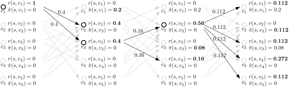
Figure 2. A running example of Forward Push on $G$ in Figure 1 with $s=v_{1}$, $\alpha=0.2$ and $r_{\max}=0.099$. The arrows are the edges of $G$ but presented in a bipartite sense. Active nodes in each iteration are highlighted in bold.

3. Preliminaries of HP-SSPPR

In this section, we introduce the details of the two most relevant existing approaches to this paper for answering Hight-Precision SSPPR queries: Power Iteration (PowItr) and Forward Push (FwdPush). In the literature, they are often considered as two different types of methods, respectively as global and local approaches. Thus, in the previous work, these two approaches are usually understood and explained from different perspectives. Next, we explain both PowItr and FwdPush from a unified perspective of alive random walks. Our explanations would hint some ideas on the equivalence connection between these two approaches as discussed in Section 4.

3.1. The Power Iteration Approach

Define $\vec{\gamma_{s}}^{(j)}\in\mathbb{R}^{1\times n}$ as the vector, of which the $i$-th coordinate is the probability that an $\alpha$-random walk from $s$ is alive at $v_{i}$ at the $j$-th step. Clearly, $\vec{\gamma_{s}}^{(0)}=\vec{e_{s}}$: a random walk from $s$ can be alive only at $s$ at the initial state, i.e., at the $0$-th step. According to the definition of $\alpha$-random walks, it can be verified that

(3) $$\small\vec{\gamma_{s}}^{(j+1)}=(1-\alpha)\cdot\vec{\gamma_{s}}^{(j)}\cdot\mathbf{P}=(1-\alpha)^{j+1}\cdot\vec{e_{s}}\cdot\mathbf{P}^{j+1}\,.$$

Therefore, the $i$-th coordinate of the vector $\alpha\cdot\vec{\gamma_{s}}^{(j)}$ is the probability that a random walk from $s$ stops at $v_{i}$ at exactly the $j$-th step.

Intuitively, by the definition of PPR, $\pi(s,t)$ can be computed as the sum of the probabilities that an $\alpha$-random walk from $s$ stops at $t$ with exactly $j$ steps, for all possible length $j=0,1,2,\cdots$. That is,

(4) $$\small\vec{\pi_{s}}=\sum_{j=0}^{\infty}\alpha\cdot\vec{\gamma_{s}}^{(j)}\,.$$

The basic idea of PowItr is to iteratively maintain an underestimate $\hat{\pi_{s}}=\vec{\pi}_{s}^{(j+1)}$ in the $(j+1)$-th iteration (for $j=0,1,2,\cdots$) such that:

(5) $$\small\vec{\pi}_{s}^{(j+1)}=\sum_{k=0}^{j}\alpha\cdot\vec{\gamma_{s}}^{(k)}\,,$$

where the $i$-th coordinate of $\vec{\pi}_{s}^{(j+1)}$ is the probability that a random walk from $s$ stops at $v_{i}$ with at most $j$ steps.

The $\ell_{1}$-Error Bound. The $\ell_{1}$-error at the end of the $(j+1)$-th iteration is given by:

$$\small\|\hat{\pi_{s}}-\vec{\pi_{s}}\|_{1} =\|\sum_{k=j+1}^{\infty}\alpha\cdot\vec{\gamma_{s}}^{(k)}\|_{1}=\sum_{k=j+1}^{\infty}\alpha\cdot(1-\alpha)^{k}\cdot\|\vec{e}_{s}\cdot\mathbf{P}^{k}\|_{1}$$

(6) $$=\sum_{k=j+1}^{\infty}\alpha\cdot(1-\alpha)^{k}\cdot\|\vec{e}_{s}\|_{1}=(1-\alpha)^{j+1}\,.$$

Two observations follow immediately from Equation (3.1). First, the $\ell_{1}$-error $(1-\alpha)^{j+1}$ is exactly equal to $\|\vec{\gamma_{s}}^{(j+1)}\|_{1}$, that is, the total probability mass of a random walk alive at the $(j+1)$-th steps. This is intuitive because this is exactly the total amount of the probability mass that is not yet converted to the PPR values. Second, the $\ell_{1}$-error decreases by a factor of $(1-\alpha)$ in each iteration; after at most $O(\log\frac{1}{\lambda})$ iterations, $\|\hat{\pi_{s}}-\vec{\pi_{s}}\|_{1}\leq\lambda$. Since it is easy to verify that the computational cost of each iteration is bounded by $O(m)$, the overall running time of PowItr is thus bounded by $O(m\cdot\log\frac{1}{\lambda})$.

3.2. The Forward Push Approach

FwdPush conceptually considers a random walk from $s$ and observes the state of this walk in terms of probability mass. Given a specified parameter $r_{\max}\in[0,1]$, the basic idea of FwdPush is to maintain, for each node $v\in V$, the following information:

• a reserve $\hat{\pi}(s,v)$: it is an underestimate of $\pi(s,v)$ and

• a residue $r(s,v)$: it is the unprocessed probability mass of the random walk from $s$ alive at $v$ at the current state.

Initially, $\hat{\pi}(s,v)=0$ for all $v\in V$ and $r(s,v)=0$ for all $v\neq s$ while $r(s,s)=1$: at the initial state, the unprocessed probability mass of the random walk from $s$ alive at $s$ is $1$.

Active Nodes. A node $v$ is active if it satisfies $r(s,v)>d_{v}\cdot r_{\max}$; otherwise, it is inactive.

The Push Operation. A crucial primitive in FwdPush is the push operation, which is to process a node’s residue. Specifically, a push operation on a node $v$ works as follows:

• First, $\alpha$ portion of $v$’s residue $r(s,v)$ is converted to $\hat{\pi}(s,v)$, i.e., $\hat{\pi}(s,v)\leftarrow\hat{\pi}(s,v)+\alpha\cdot r(s,v)$. This represents the fact that with probability $\alpha$, the alive random walk at $v$ stops at $v$.

• Second, the rest $(1-\alpha)$ portion of $r(s,v)$ is evenly distributed to the residues of $v$’s out-neighbors. That is, the residue of each out-neighbor of $v$ is increased by $\frac{(1-\alpha)\cdot r(s,v)}{d_{v}}$, which is the probability that, conditioned on $r(s,v)$, the random walk at $v$ moves to this out-neighbor and is alive at this out-neighbor at the current state.

• Third, after the residue of $v$ is processed, $r(s,v)\leftarrow 0$, indicating that currently there is no unprocessed probability mass of the random walk from $s$ currently alive at $v$.

The process of FwdPush is to repeatedly pick an arbitrary active node, and perform a push operation on it. The algorithm terminates until there is no active node. Algorithm 1 shows the pseudo-code.

Input: $G$, $\alpha$, $s$, $r_{\max}$

Output: an estimation $\hat{\pi_{s}}$ of $\vec{\pi_{s}}$

1 $\hat{\pi}(s,v)\leftarrow 0$ and $r(s,v)\leftarrow 0$ for all $v\in V$; $r(s,s)\leftarrow 1$;

2 while there exists a node $v$ with $r(s,v)>d_{v}\cdot r_{\max}$ do

3       pick an arbitrary such node $v$ with $r(s,v)>d_{v}\cdot r_{\max}$;

4       $\hat{\pi}(s,v)\leftarrow\hat{\pi}(s,v)+\alpha\cdot r(s,v)$;

5       for each $u\in N_{out}(v)$ do

6             $r(s,u)\leftarrow r(s,u)+\frac{(1-\alpha)\cdot r(s,v)}{d_{v}}$;

7            

8      $r(s,v)\leftarrow 0$;

9      

10return $\hat{\pi}(s,v)$ for all $v\in V$ as a vector $\hat{\pi_{s}}$;

Algorithm 1 Forward Push

A Running Example. Figure 2 shows a running example. At the beginning, only $v_{1}$ is active; thus it is picked to perform a push operation, in which $\hat{\pi}(s,v_{1})=\alpha\cdot 1=0.2$ and the residues of $v_{1}$’s out-neighbors $v_{2}$ and $v_{3}$ are increased by $(1-\alpha)\cdot 1/2=0.4$, respectively. After this push operation on $v_{1}$, both $v_{2}$ and $v_{3}$ are now active. The algorithm picks one of them arbitrarily; in this example, $v_{3}$ is picked. After the push operation on $v_{3}$, $\hat{\pi}(s,v_{3})=0.2\cdot 0.4=0.08$ and each of its out-neighbors, i.e., $v_{2}$ and $v_{4}$, has residue increased by $0.8\cdot 0.4/2=0.16$. Next, $v_{2}$ becomes the only active node; after the push operation on $v_{2}$, no node is active and thus the algorithm terminates.

The $\ell_{1}$-Error Bound. When FwdPush terminates, it holds that $r(s,v)\leq d_{v}\cdot r_{\max}$ for all $v\in V$. By definition, the residues are the probability mass of the alive random walk that are not yet converted to $\hat{\pi}(s,v)$’s. Hence,

(7) $$\small\|\hat{\pi_{s}}-\vec{\pi_{s}}\|_{1}=\sum_{v\in V}r(s,v)\leq\sum_{v\in V}d_{v}\cdot r_{\max}=m\cdot r_{\max}\,.$$

In order to achieve an $\ell_{1}$-error at most $\lambda$, one needs to set $r_{\max}\leq\frac{\lambda}{m}$.

The Open Question. The only known time complexity of FwdPush is $O(\frac{1}{r_{\max}})$ (Andersen et al., 2006). Unfortunately, this bound implies that the overall running time becomes $O(\frac{m}{\lambda})$ with $r_{\max}=\lambda/m$, which is worse than the $O(m\cdot\log\frac{1}{\lambda})$-bound of PowItr. Despite of its practicality in certain applications, it still remains an open question: Does FwdPush admit a running time bound with a weaker dependency on $\lambda$, just like what PowItr does?

4. A Tighter Analysis of Forward Push

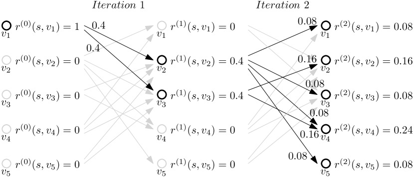
Figure 3. A running example of SimFwdPush on $G$ with $s=v_{1}$, $\alpha=0.2$ and $r_{\max}=0$. Active nodes are highlighted in bold.

In this section, we give a positive answer to the open question regarding to the running time of FwdPush. More specifically, we prove that under a proper strategy to pick active nodes to perform push operations, the overall running time of FwdPush can be bounded by $O(m\cdot\log\frac{1}{\lambda})$ with $r_{\max}=\lambda/m$. This finding stems from an observation on a subtle equivalence connection between PowItr and FwdPush as we discuss next.

4.1. Equivalence Connection to Power Iteration

Recall that in each iteration, PowItr essentially computes $\vec{\gamma_{s}}^{(j+1)}=(1-\alpha)\cdot\vec{\gamma_{s}}^{(j)}\cdot\mathbf{P}$. Thus, the alive random walks considered in the same iteration are all with the same lengths. Such a well structured process makes the error bound analysis of PowItr relatively clear. In contrast, the process of FwdPush is a lot less structured. Due to the fact that FwdPush allows to perform push operations on arbitrary active nodes, the residues of the nodes actually mix up the probability mass of the alive random walk from $s$ at the states of different lengths. Despite of the similar rationale of moving alive random walks one-step forward in both of the algorithms, the arbitrary push operation ordering of FwdPush makes the analysis of the error bound during the algorithm very challenging. To overcome this challenge, we conceptually restrict FwdPush to perform push operations in iterations.

A Special FwdPush Variant. As the first step, we reveal the subtle equivalence connection between PowItr and FwdPush. In the following, we show a special variant of FwdPush which can perform exactly the same computation for $\vec{\gamma_{s}}^{(j+1)}$ and $\vec{\pi_{s}}^{(j+1)}$ in PowItr. This variant is called Simultaneous Forward Push (SimFwdPush), and has the following modifications on Algorithm 1:

• All the nodes with non-zero residues are active, i.e., $r_{\max}=0$.

• The SimFwdPush algorithm works in iterations:

  • At the beginning of the $(j+1)$-th iteration (for integer $j\geq 0$), the residue of node $v$ is denoted by $r^{(j)}(s,v)$.

  • In each iteration, the algorithm performs a push operation on every active node simultaneously based on $r^{(j)}(s,v)$.

• At the end of the $(j+1)$-th iteration, the algorithm terminates if the $\ell_{1}$-error $r_{sum}=\sum_{v\in V}r^{(j+1)}(s,v)\leq\lambda$.

A Running Example. Figure 3 shows a running example of SimFwdPush. At the beginning of the first iteration, only $v_{1}$ has non-zero residue, i.e., $r^{(0)}(s,v_{1})=1$, and thus, it is the only active node in this iteration. After the push operation on $v_{1}$ $r^{(1)}(s,v_{2})=r^{(1)}(s,v_{3})=\frac{(1-\alpha)\cdot r^{(0)}(s,v_{1})}{d_{v_{1}}}=0.4$. Hence, $v_{2}$ and $v_{3}$ are the two active nodes in the second iteration. The algorithm then performs push operations simultaneously on both $v_{2}$ and $v_{3}$, where the operation on $v_{2}$ pushes $\frac{(1-\alpha)\cdot r^{(1)}(s,v_{2})}{d_{v_{2}}}=0.08$ probability mass to each $v_{2}$’s out-neighbor, while the operation on $v_{3}$ pushes $\frac{(1-\alpha)\cdot r^{(1)}(s,v_{3})}{d_{v_{3}}}=0.16$ to its out-neighbors accordingly. The resulted residue of each node is shown in the figure.

The Connection. Define $\vec{r_{s}}^{(j)}\in\mathbb{R}^{1\times n}$ as the residue vector of all the nodes, whose the $i$-th coordinate is $r^{(j)}(s,v_{i})$. The crucial observation on SimFwdPush is that performing simultaneous push operations on all the active nodes in the $(j+1)$-th iteration is equivalent to the following computation:

$$\vec{r_{s}}^{(j+1)} =\sum_{\text{active}\,v}\frac{(1-\alpha)\cdot r^{(j)}(s,v)}{d_{v}}\cdot\vec{A}_{v}=\sum_{v\in V}\frac{(1-\alpha)\cdot r^{(j)}(s,v)}{d_{v}}\cdot\vec{A}_{v}$$

$$=\sum_{v\in V}(1-\alpha)\cdot r^{(j)}(s,v)\cdot\vec{P}_{v}=\sum_{v\in V}\left((1-\alpha)\cdot r^{(j)}(s,v)\cdot\vec{e}_{v}\cdot\mathbf{P}\right)$$

(8) $$=(1-\alpha)\cdot\left(\sum_{v\in V}r^{(j)}(s,v)\cdot\vec{e}_{v}\right)\cdot\mathbf{P}=(1-\alpha)\cdot\vec{r_{s}}^{(j)}\cdot\mathbf{P}\,.$$

We have the following lemmas.

Lemma 4.1.

The residue vector $\vec{r_{s}}^{(j+1)}$ and underestmate PPR vector $\hat{\pi_{s}}^{(j+1)}$ obtained by SimFwdPush in the $(j+1)$-th iteration are exactly the same as $\vec{\gamma_{s}}^{(j+1)}$ and $\vec{\pi}_{s}^{(j+1)}$ computed in the $(j+1)$-th iteration in PowItr, for all integer $j\geq 0$.

Proof.

We prove this lemma with a mathematical induction argument. Clearly, the base case $\vec{r_{s}}^{(0)}=\vec{\gamma_{s}}^{(0)}=\vec{e}_{s}$ and $\hat{\pi_{s}}^{(0)}=\vec{\pi_{s}}^{(0)}=\vec{0}$ holds. For the inductive case, assuming that $\vec{r_{s}}^{(j)}=\vec{\gamma_{s}}^{(j)}$ and $\hat{\pi_{s}}^{(j)}=\vec{\pi_{s}}^{(j)}$ holds, by Equation (4.1), we have:

$$\vec{r_{s}}^{(j+1)}=(1-\alpha)\cdot\vec{r_{s}}^{(j)}\cdot\mathbf{P}=(1-\alpha)\cdot\vec{\gamma_{s}}^{(j)}\cdot\mathbf{P}=\vec{\gamma_{s}}^{(j+1)}\,;$$

and according to the push operations,

$$\hat{\pi_{s}}^{(j+1)}=\hat{\pi_{s}}^{(j)}+\alpha\cdot\vec{r_{s}}^{(j)}=\sum_{k=0}^{j}\alpha\cdot\vec{r_{s}}^{(k)}=\sum_{k=0}^{j}\alpha\cdot\vec{\gamma_{s}}^{(k)}=\vec{\pi_{s}}^{(j+1)}\,.$$

Therefore, the inductive case holds, and the lemma follows. ∎

Lemma 4.2.

The overall running time of SimFwdPush is bounded by $O(m\cdot\log\frac{1}{\lambda})$.

Proof.

The cost of each push operation on a node $v$ is $O(d_{v})$. Thus, in each iteration, the total cost is bounded by the total degree $O(\sum_{v\in V}d_{v})=O(m)$. According to the analysis of PowItr and Lemma 4.1, after at most $O(\log\frac{1}{\lambda})$ iterations, the $\ell_{1}$-error $r_{sum}\leq\lambda$. ∎

Putting Lemmas 4.1 and  4.2 together, we conclude that: SimFwdPush is equivalent to PowItr.

4.2. A Tighter Analysis

Unfortunately, the equivalence between SimFwdPush and PowItr is not sufficient to answer the open question regarding to the running time of FwdPush. The reasons are as follows:

• First, the push operations in SimFwdPush are performed simultaneously in each iteration, while in FwdPush, they are performed in an asynchronous way.

• Second, the crucial parameter $r_{\max}$ does not make much effect in SimFwdPush, but it determines which node is eligible for a push operation in FwdPush.

• Third, the stop condition in SimFwdPush that requires $r_{sum}\leq\lambda$ is not a sufficient condition to achieve $r(s,v)\leq d_{v}\cdot r_{\max}$ for all $v\in V$, where the latter is the original stop condition in FwdPush.

In this subsection, we remove all these restrictions. The only requirement in our analysis for FwdPush is that the algorithm is performed in iterations (just as what SimFwdPush does and as defined below). We note that considering the algorithm in iterations makes the entire process more structured and thus allows us to bound the decrease rate of the $\ell_{1}$-error. Nonetheless, as mentioned earlier, such a requirement is not a strong restriction; and it indeed can be implemented as simple as with a First-In-First-Out queue to organize the active nodes during the algorithm. Interestingly enough, this is actually a common implementation of FwdPush in practice – people have unconsciously implemented FwdPush in an efficient way! From our analysis, it explains why FwdPush is often found to have a weaker dependency on $\lambda$ than as what its previous running time complexity suggested in applications.

Input: $G$, $\alpha$, $s$, $r_{\max}$

Output: an estimation $\hat{\pi_{s}}$ of $\vec{\pi_{s}}$ and the resulted residues $\vec{r_{s}}$

1 $\hat{\pi}(s,v)\leftarrow 0$ and $r(s,v)\leftarrow 0$ for all $v\in V$; $r(s,s)\leftarrow 1$;

2 initialize a first-in-first-out queue $Q\leftarrow\emptyset$;

3 $Q.append(s)$; // append $s$ at the end of $Q$;

4 while $Q\neq\emptyset$ do

5       $v\leftarrow Q.pop()$; // pop and remove the front node from $Q$;

6       $\hat{\pi}(s,v)\leftarrow\hat{\pi}(s,v)+\alpha\cdot r(s,v)$;

7       for each $u\in N_{out}(v)$ do

8             $r(s,u)\leftarrow r(s,u)+\frac{(1-\alpha)\cdot r(s,v)}{d_{v}}$;

9             if $r(s,u)>d_{u}\cdot r_{\max}$ and $u\not\in Q$ then

10                   // $u$ is active and not in $Q$;

11                   $Q.append(u)$; // append $u$ at the end of $Q$;

12                  

13            

14      $r(s,v)\leftarrow 0$;

15      

16return $\hat{\pi}(s,v)$ for all $v\in V$ as a vector $\hat{\pi_{s}}$, and $r(s,v)$ for all $v\in V$ as the resulted residue vector $\vec{r_{s}}$;

Algorithm 2 First-In-First-Out Forward Push

In the following, we analyse the running time of an implementation of FwdPush, called First-In-First-Out Forward Push (FIFO-FwdPush), whose pseudo-code is shown in Algorithm 2. We answer the open question regarding to the running time of FwdPush by proving the following theorem.

Theorem 4.3.

Given $0<r_{\max}<\frac{1}{2\cdot m}$ and $\lambda=m\cdot r_{\max}$, the overall running time of FIFO-FwdPush is bounded by $O(m\cdot\log\frac{1}{\lambda})$.

It should be noted that when $r_{\max}\geq\frac{1}{2\cdot m}$, the bound $O(\frac{1}{r_{\max}})=O(m)$ is already good enough. Furthermore, as aforementioned, the goal is to obtain high-precision results; the $\lambda$ value of interest is often even smaller than $10^{-8}$ and thus, $r_{\max}$ is often far smaller than $\frac{1}{2\cdot m}$ in practice.

The Iterations. For the ease of analysis, we first define the iterations of FIFO-FwdPush based on Algorithm 2. In particular, we define $S^{(j)}$ as the set of all the active nodes at the beginning of the $(j+1)$-th iteration, where $j=0,1,2,\cdots$. Specifically, we define $S^{(j)}$ in an inductive way:

• Initially, $S^{(0)}=\{s\}$: the source node is the only active node at the beginning of the first iteration.

• $S^{(j+1)}$ is the set of all the nodes appended to $Q$ at Line $11$ in Algorithm 2 when processing the nodes in $S^{(j)}$.

Furthermore, in the $(j+1)$-th iteration, the algorithm performs a push operation for every active node in $S^{(j)}$.

Under this definition, the iterations are exactly the same as those we considered in SimFwdPush, except that the push operations are now performed in an asynchronous way. Consider the example in Figure 3 and assume $r_{\max}$ is sufficiently small, e.g., $0.001$; $S^{(0)}$ contains $v_{1}$ only. After the push operation on $v_{1}$, only $v_{2}$ and $v_{3}$ are appended to $Q$; thus, $S^{(1)}=\{v_{2},v_{3}\}$. In the second iteration, during the push operations on $v_{2}$ and $v_{3}$, all the five nodes are appended to $Q$. Hence, $S^{(2)}=\{v_{1},v_{2},v_{3},v_{4},v_{5}\}$.

An Overview of the Analysis. Let $r_{\text{sum}}^{(j)}=\|\vec{r_{s}}^{(j)}\|_{1}$, the total residues of all the nodes at the beginning of the $(j+1)$-th iteration. Initially, $r_{\text{sum}}^{(0)}=1$. According to the analysis for FwdPush, we know that $r_{\text{sum}}^{(j+1)}$ is exactly the $\ell_{1}$-error after the $(j+1)$-th iteration. When the iteration number is not important, we use $r_{\text{sum}}$ to denote the $\ell_{1}$-error at the current state.

Our analysis on the overall running time of FIFO-FwdPush consists of two main steps. Firstly, we show that the following lemma:

Lemma 4.4.

In $O(m\cdot\log\frac{1}{\lambda}+m)$ time, FIFO-FwdPush can make the $\ell_{1}$-error $r_{\text{sum}}\leq\lambda$.

As aforementioned, $r_{\text{sum}}\leq\lambda$ is not sufficient to guarantee that $r(s,v)\leq d_{v}\cdot r_{\max}$ holds for all $v\in V$. Thus, the FIFO-FwdPush algorithm may not stop and keep running until there is no more active node. To bound the running time of this part, in the second step, we prove:

Lemma 4.5.

Starting from the state of $r_{\text{sum}}\leq\lambda$, FIFO-FwdPush stops in $O(m)$ time.

Theorem 4.3 follows immediately from these two lemmas. In the rest of this subsection, we prove Lemmas 4.4 and  4.5, respectively.

Proof of Lemma 4.4. Consider the $(j+1)$-th iteration; FIFO-FwdPush performs a push operation on each node $v\in S^{(j)}$. For each such push operation, an amount of $\alpha\cdot r^{(j)}(s,v)$ probability mass is converted to $\hat{\pi}^{(j+1)}(s,v)$, and hence, $r_{\text{sum}}^{(j)}$ is decreased by $\alpha\cdot r^{(j)}(s,v)$. Therefore, at the end of this $(j+1)$-th iteration, the net decrease of $r_{\text{sum}}^{(j)}$ is:

(9) $$\small r_{\text{sum}}^{(j)}-r_{\text{sum}}^{(j+1)}\geq\alpha\cdot\sum_{v\in S^{(j)}}r^{(j)}(s,v)\,.$$

The key in our proof is to show $r_{\text{sum}}^{(j+1)}\leq(1-\frac{\alpha}{m}\cdot\sum_{v\in S^{(j)}}d_{v})\cdot r_{\text{sum}}^{(j)}$. To achieve this, we show the following observation.

Observation 1.

$\sum_{v\in S^{(j)}}r^{(j)}(s,v)\geq\frac{1}{m}\cdot\sum_{v\in S^{(j)}}d_{v}\cdot r_{\text{sum}}^{(j)}\,$.

Proof.

In the following calculation, we omit all the superscripts in $S^{(j)}$, $r_{\text{sum}}^{(j)}$ and the residues $r^{(j)}(s,v)$ as they are all with respect to $j$. Clearly, when $\sum_{v\in S}d_{v}=0$ or $\sum_{v\in S}d_{v}=m$, the observation holds. Otherwise, by the definition of active nodes, we have:

$$\frac{\sum_{v\in S}r(s,v)}{\sum_{v\in S}d_{v}}\geq r_{\max}\geq\frac{\sum_{v\not\in S}r(s,v)}{\sum_{v\not\in S}d_{v}}\,.$$

Therefore, it follows that:

$$\frac{\sum_{v\in S}r(s,v)}{\sum_{v\in S}d_{v}}\geq\frac{\sum_{v\in S}r(s,v)+\sum_{v\notin S}r(s,v)}{\sum_{v\in S}d_{v}+\sum_{v\notin S}d_{v}}=\frac{r_{sum}}{m}\,.$$

The observation follows. ∎

Substituting Observation 1 to Equation (9), we have:

$$r_{\text{sum}}^{(j+1)} \leq r_{\text{sum}}^{(j)}-\alpha\sum_{v\in S^{(j)}}r^{(j)}(s,v)\leq(1-\frac{\alpha}{m}\cdot\sum_{v\in S^{(j)}}d_{v})\cdot r_{\text{sum}}^{(j)}$$

$$\leq\prod_{k=0}^{j}(1-\frac{\alpha}{m}\cdot\sum_{v\in S^{(k)}}d_{v})\cdot r_{\text{sum}}^{(0)}$$

(10) $$\leq\exp\left(-\sum_{k=0}^{j}(\frac{\alpha}{m}\cdot\sum_{v\in S^{(k)}}d_{v})\right)=\exp\left(-\frac{\alpha}{m}\cdot(\sum_{k=0}^{j}\sum_{v\in S^{(k)}}d_{v})\right)\,,$$

where the last inequality follows from the fact that $1-x\leq e^{-x}$ holds for all $x\in\mathbb{R}$.

Let $T^{(j+1)}=\sum_{k=0}^{j}\sum_{v\in S^{(k)}}d_{v}$ be the total degree of the node in each push operation performed in the first $(j+1)$ iterations. By Equation (4.2), in order to make $r_{\text{sum}}^{(j+1)}\leq\lambda$, it suffices to find the smallest $j$ such that

$$\exp\left(-\frac{\alpha}{m}\cdot T^{(j+1)}\right)\leq\lambda\leq\exp\left(-\frac{\alpha}{m}\cdot T^{(j)}\right)\,.$$

Thus, we have:

$$T^{(j)}\leq\frac{m}{\alpha}\cdot\ln\frac{1}{\lambda}\leq T^{(j+1)}\,.$$

By the fact that $T^{(j+1)}-T^{(j)}=\sum_{v\in S^{(j)}}d_{v}\leq m$, we further have:

(11) $$T^{(j+1)}\leq T^{(j)}+m\leq\frac{m}{\alpha}\cdot\ln\frac{1}{\lambda}+m\,.$$

Finally, since the cost of a push operation on $v$ is bounded by $O(d_{v})$, thus $O(T^{(j+1)})$ is actually an upper bound on the overall cost in the first $(j+1)$ iterations. Therefore, the overall running time to achieve $r_{\text{sum}}^{(j+1)}\leq\lambda$ is bounded by $O(m\cdot\log\frac{1}{\lambda}+m)$. This completes the whole proof for Lemma 4.4.

Proof of Lemma 4.5. Let $r_{\text{sum}}^{\text{before}}=r_{\text{sum}}^{(j+1)}\leq\lambda$ be the $r_{\text{sum}}$ at the current state, and $r_{\text{sum}}^{\text{after}}$ be the $r_{\text{sum}}$ when the algorithm terminates. Recall that each push operation on an active node $v$ decreases $r_{\text{sum}}$ by $\alpha\cdot r(s,v)\geq\alpha\cdot d_{v}\cdot r_{\max}$, and the corresponding running time cost is $O(d_{v})$. Therefore, after paying a total running time cost of $O(T)$, the net decrease of $r_{\text{sum}}$ is at least $\alpha\cdot T\cdot r_{\max}$. As the net decrease is at most $r_{\text{sum}}^{\text{before}}-r_{\text{sum}}^{\text{after}}\leq\lambda$, it follows that $\alpha\cdot T\cdot r_{\max}$ cannot be greater than $\lambda$. Hence, $T\leq\frac{\lambda}{\alpha\cdot r_{\max}}=O(m)$. Thus, the largest possible running time of FIFO-FwdPush starting from the state of $r_{\text{sum}}\leq\lambda$ is bounded by $O(m)$. Lemma 4.5 thus follows.

5. A New Efficient Power Iteration

In the previous section, we show that: (i) PowItr is equivalent to a special variant of FwdPush, and (ii) a simple implementation FIFO-FwdPush of FwdPush can achieve time complexity $O(m\cdot\log\frac{1}{\lambda})$. Based on these theoretical findings, in this section, we design an efficient implementation of PowItr, call Power Iteration with Forward Push (PowerPush), from an engineering point of view. Our optimizations in the design of PowerPush unifies the global-approach PowItr and local-approach FwdPush and incorporates both their strengths. Algorithm 3 is the pseudo-code of PowerPush. We introduce some crucial optimizations in PowerPush in below.

Asynchronous Pushes. Unlike PowItr, our PowerPush uses asynchronous push operations. We note that asynchronous push operations can be possibly more effective. This is because during the $(j+1)$-th iteration, if there is a push operation on an in-neighbor $u$ of a node $v$ before the push of $v$, when $v$ pushes, its current residue is greater than $r^{(j)}(s,v)$, and hence, this push operation can send out more residue. To see this, in the second iteration in Figure 3, the simultaneous push operation on $v_{2}$ is performed based on a residue of $0.4$ but in the same iteration in Figure 2, the push on $v_{2}$ is based on a residue of $0.56$. This is because $v_{3}$ pushed before $v_{2}$, and hence, $v_{2}$’s residue has been increased by $0.16$. Moreover, after this asynchronous push, the residue of $v_{2}$ becomes $0$ in the next iteration, while in contrast, $v_{2}$ still has $0.16$ (obtained from $v_{3}$) under the simultaneous pushes. In other words, this asynchronous push on $v_{2}$ has equivalently processed the residues of $v_{2}$ in two iterations under simultaneous pushes.

Global Sequential Scan v.s. Local Random Access. One of the biggest optimizations in PowerPush is the strategy of switching to a global sequential scan from using the queue to access active nodes. The key observation is that after a few iterations, in FIFO-FwdPush, there would be a large number of active nodes which are stored in the queue according to their “append-to-queue” order. As a result, to perform push operations on these nodes, it requires a large number of random access in both the node list and the edge list, incurring a substantial overhead.

To remedy this, in PowerPush, when the current number of active nodes is greater than a specified $scanThreshold$, it switches to sequential scan the node list to perform push operations on the active nodes (as shown in Algorithm 3 Line $15$ - $24$). Moreover, to further facilitate this idea, PowerPush stores all the nodes sorted by id’s and concatenates the adjacent lists of the nodes in the same order (i.e., sorted by id’s) in a large array. Thanks to this storage format, in each iteration, PowerPush can perform push operations on active nodes via a sequential scan on this edge array, which in turn has largely make the memory access patterns become cache-friendly. Interestingly, this idea is borrowed from the implementation of PowItr as a global-approach.

Dynamic $\ell_{1}$-Error Threshold. Another optimization worth mentioning is the strategy of using dynamic $\ell_{1}$-error threshold (see Line $17$ in Algorithm 3). The rationale here is that with a larger $\ell_{1}$-error threshold, it allows us to use a larger $r_{\max}$. We note that $r_{\max}$ essentially specifies a threshold on the unit-cost benefit of the push operations. To see this, recall that a push operation on $v$ takes $O(d_{v})$ cost and reduces $r_{\text{sum}}$ by $\alpha\cdot r(s,v)$. Thus, $\alpha\cdot r(s,v)/d_{v}$ can be considered as the unit-cost benefit of this operation. By definition, a node becomes active only if a push operation on it has unit-cost benefit $\geq\alpha\cdot r_{\max}$. The good thing of performing push operations with higher unit-cost benefits first is that it allows other nodes to accumulate their residues before pushing. In this way, the number of push operations to achieve $\ell_{1}$-error can be considerably reduced. Motivated by this, we perform PowerPush in epochs. In the $i$-th ($1\leq i\leq epochNum$) epoch, an $\ell_{1}$-error $\lambda^{\frac{i}{epochNum}}\geq\lambda$ is adopted to perform those push operations with higher unit-cost benefits.

Remark. The $\hat{\pi_{s}}$ and $\vec{r_{s}}$ returned by PowerPush can be further refined to ensure $r(s,v)\leq d_{v}\cdot r_{\max}$, where $r_{\max}=\frac{\lambda}{m}$, holds for all $v\in V$. By Lemma 4.5, such refinement only takes $O(m)$ time.

Input: $G$, $\alpha$, $s$, $\lambda$

Output: an estimation $\hat{\pi_{s}}$ of $\vec{\pi_{s}}$ and the resulted residues $\vec{r_{s}}$

1 $epochNum=8$; // a tunable constant;

2 $scanThreshold=n/4$; // a threshold to use sequential scan;

3 $\hat{\pi}(s,v)\leftarrow 0$ and $r(s,v)\leftarrow 0$ for all $v\in V$; $r(s,s)\leftarrow 1$;

4 initialize a first-in-first-out queue $Q\leftarrow\emptyset$;

5 $Q.append(s)$;

6 $r_{\max}\leftarrow\lambda/m$;

7 while $Q\neq\emptyset$ and $Q$.size() $\leq$ $scanThreshold$ and $r_{\text{sum}}>\lambda$ do

8       $v\leftarrow Q.pop()$;

9       $\hat{\pi}(s,v)\leftarrow\hat{\pi}(s,v)+\alpha\cdot r(s,v)$;

10       for each $u\in N_{out}(v)$ do

11             $r(s,u)\leftarrow r(s,u)+\frac{(1-\alpha)\cdot r(s,v)}{d_{v}}$;

12             if $u\not\in Q$ is active w.r.t. $r_{\max}$, $Q.append(u)$;

13            

14      $r(s,v)\leftarrow 0$;

15      

16if $r_{\text{sum}}>\lambda$ then

17       // Switch to using sequential scan;

18       for $i\leftarrow 1;i\leq epochNum;i\leftarrow i+1$ do

19             $r_{\max}^{\prime}\leftarrow\lambda^{\frac{i}{epochNum}}/m$; // allow a larger $\ell_{1}$-error;

20             while $r_{\text{sum}}>m\cdot r_{\max}^{\prime}$ do

21                   for each $v\in V$ do

22                         if $v$ is active w.r.t. $r_{\max}^{\prime}$ then

23                               $\hat{\pi}(s,v)\leftarrow\hat{\pi}(s,v)+\alpha\cdot r(s,v)$;

24                               for each $u\in N_{out}(v)$ do

25                                     $r(s,u)\leftarrow r(s,u)+\frac{(1-\alpha)\cdot r(s,v)}{d_{v}}$;

26                                    

27                              $r(s,v)\leftarrow 0$;

28                              

29                        

30                  

31            

32      

33return $\hat{\pi}(s,v)$ for all $v\in V$ as a vector $\hat{\pi_{s}}$, and $r(s,v)$ for all $v\in V$ as the resulted residue vector $\vec{r_{s}}$;

Algorithm 3 Power Iteration with Forward Push

6. Improved Approx-SSPPR Algorithm

In this section, we propose a new algorithm, called SpeedPPR, for answering approximate SSPPR queries.

6.1. Preliminaries on Approx-SSPPR

In this subsection, we first introduce some preliminaries on two relevant algorithms: MonteCarlo and FORA. The ideas of these two algorithms would help understand the key idea of the design of our SpeedPPR. Recall that an Approx-SSPPR query aims to compute an estimation $\hat{\pi}(s,v)$ for every node $v$ with $\pi(s,v)\geq\mu$ within relative error $\epsilon$ with a succeed probability at least $1-\frac{1}{n}$.

The Monte Carlo Method. Perhaps, one of the most straightforward ways to answer Approx-SSPPR query is the MonteCarlo method. The basic idea is to generate $W$ independent $\alpha$-random walks from $s$, and utilise the empirical number $f(s,v)$ out of these random walks that stop at a node $v$ to estimate its expectation $\pi(s,v)\cdot W$. Thus, $\hat{\pi}(s,v)=\frac{f(s,v)}{W}$ gives an estimation of $\pi(s,v)$. By the standard Chernoff Bound (Chung and Lu, 2006), it is known that setting

(12) $$W=\frac{2\cdot(2\cdot\epsilon/3+2)\cdot\log n}{\epsilon^{2}\cdot\mu}=O(\frac{\log n}{\epsilon^{2}\cdot\mu})$$

suffices to obtain a correct estimation for every node $v$ with $\pi(s,v)\geq\mu$ with probability at least $1-\frac{1}{n}$. Furthermore, as the expected length of an $\alpha$-random walk is at most $\frac{1}{\alpha}$, the overall expected running time of MonteCarlo is bounded by $O(\frac{\log n}{\epsilon^{2}\cdot\mu})$. When $\mu=\frac{1}{n}$, this bound can be written as $O(\frac{n\cdot\log n}{\epsilon^{2}})$.

In the rest of this section, without loss of generality, we assume that $m<W$, because otherwise, i.e., $m\geq W$, one can always switch their algorithm to the MonteCarlo method and guarantee a time complexity $O(W)$ no worse than $O(m)$.

FORA. FORA (Wang et al., 2017) is a state-of-the-art representative algorithm for answering Approx-SSPPR queries. It adopts a two-phase framework and combines FwdPush and MonteCarlo. In the first phase, it runs FwdPush with a specified $r_{\max}$ (whose value is to be determined shortly) to obtain an estimation $\hat{\pi_{s}}$ of $\vec{\pi_{s}}$ with $\|\hat{\pi_{s}}-\vec{\pi_{s}}\|_{1}=r_{\text{sum}}=\sum_{v\in V}r(s,v)\leq m\cdot r_{\max}$. In the second phase, it performs the MonteCarlo method. Specifically, it works as follows. For each node $v$ with $r(s,v)>0$, FORA generates $W_{v}=\lceil r(s,v)\cdot W\rceil$ random walks from $v$, where $W$ is set by Equation (12). Among these $W_{v}$ random walks from $v$, if $f(v,u)$ out of them had stopped at a node $u$, then increase $\hat{\pi}(s,u)$ by:

(13) $$\frac{r(s,v)\cdot W}{W_{v}}\cdot\frac{f(v,u)}{W}=r(s,v)\cdot\frac{f(v,u)}{W_{v}}\,.$$

In summary, the final estimation $\hat{\pi}^{\prime}(s,u)$ of $\pi(s,u)$ is computed as:

(14) $$\hat{\pi}^{\prime}(s,u)=\hat{\pi}(s,u)+\sum_{v\in V:r(s,v)>0}r(s,v)\cdot\frac{f(v,u)}{W_{v}}\,,$$

where $\hat{\pi}(s,u)$ is obtained in the first FwdPush phase, and the second term is the net increase based on $\hat{\pi}(s,u)$ in the MonteCarlo phase.

Running Time Analysis. According to the previous bound on the running time of FwdPush, the cost of the first phase in FORA is bounded by $O(\frac{1}{r_{\max}})$; and in the second phase, FORA needs to generate at most $\sum_{v\in V:r(s,v)>0}\lceil r(s,v)\cdot W\rceil\leq r_{\text{sum}}\cdot W+n\leq m\cdot r_{\max}\cdot W+n$ random walks. Therefore, the overall expected time of FORA is bounded by $O(\frac{1}{r_{\max}}+m\cdot r_{\max}\cdot W+n)$, which can be minimized to $O(\sqrt{m\cdot W}+n)$ by setting $r_{\max}=\frac{1}{\sqrt{m\cdot W}}$. When $\mu=\frac{1}{n}$ and the graph is scale-free, i.e., $m=O(n\cdot\log n)$, this bound can be further simplified to $O(\frac{n\cdot\log n}{\epsilon})$. In this case, FORA improves the MonteCarlo method by a factor of $\frac{1}{\epsilon}$, Furthermore, this $O(\frac{n\cdot\log n}{\epsilon})$-bound is actually state-of-the-art; none of the existing algorithms can overcome this barrier.

Pre-Computing the Random Walks. An optimization of FORA is to pre-compute $K_{v}$ random walks for each node $v\in V$, where $K_{v}=d_{v}\cdot\sqrt{\frac{W}{m}}+1\geq W_{v}$; when answering a query, it just needs to read the pre-computed random walk results to perform the second MonteCarlo phase. Therefore, the actual query cost can be further reduced. Such an index-based variant is called FORA+. The space consumption of all the pre-computed random walk results is $\sum_{v\in V}K_{v}=\sqrt{m\cdot W}+n$. When $m=O(n\cdot\log n)$, this gives the overall space consumption bound $O(\frac{1}{\epsilon}\cdot n\cdot\log n)$. Unfortunately, as the number of pre-computed random walks for each node depends on $W$ and hence on the relative error $\epsilon$, the index of FORA+ constructed for an $\epsilon=\epsilon_{1}$ is not sufficient to answer queries with relative error $\epsilon_{2}<\epsilon_{1}$. Moreover, to support queries with small $\epsilon$, the index requires a substantial space consumption. These drawbacks have significantly limited the applicability of FORA+.

6.2. Our Improved Algorithm

Next, we propose a new Approx-SSPPR algorithm, called SpeedPPR, which not only improves FORA’s running time complexity, but also admits an index with size independent to $\epsilon$. While it eventually turns out that SpeedPPR is as simple as substituting PowerPush along with a $O(m)$-time post-refinement (to ensure that no node is active with respect to $r_{\max}=\frac{1}{W}$) in the first phase of FORA, it is our new PowerPush technique to make these improvements of SpeedPPR over FORA become possible. The pseudo-code of SpeedPPR is shown in Algorithm 4.

Theorem 6.1.

The overall expected running time of SpeedPPR is bounded by $O(m\cdot\log\frac{W}{m})$, where $W$ is computed as Equation (12). When the graph is scale-free, i.e., $m=O(n\cdot\log n)$ and $\mu=\frac{1}{n}$, this bound can be written to $O(n\cdot\log n\cdot\log\frac{1}{\epsilon})$.

Proof.

The correctness of SpeedPPR follows immediately from FORA. It thus suffices to bound the expected running time.

In the first phase, the cost of running PowerPush with $r_{\max}=\frac{1}{W}$ is bounded by $O(m\cdot\log\frac{W}{m}+m)$. In the second phase, for each node $v$ with $r(s,v)>0$, SpeedPPR needs to perform $W_{v}=\lceil r(s,v)\cdot W\rceil\leq\lceil d_{v}\cdot r_{\max}\cdot W\rceil=d_{v}$ random walks. Thus, in total, there are at most $m$ random walks needed, and hence, the expected running time for performing them is $O(m)$. Putting the two cost together, the overall expected running time of SpeedPPR is bounded by $O(m\cdot\log\frac{W}{m})$. Furthermore, when $m=O(n\cdot\log n)$ and $\mu=\frac{1}{n}$, the bound is simplified to $O(n\cdot\log n\cdot\log\frac{1}{\epsilon})$. ∎

Improvements over FORA. Despite of the analogous algorithm framework, SpeedPPR has two significant improvements over FORA.

• First, the overall expected running time of SpeedPPR improves FORA’s state-of-the-art $O(\frac{1}{\epsilon}\cdot n\cdot\log n)$-bound by almost a factor of $\frac{1}{\epsilon}$. Given the importance of Approx-SSPPR queries, our improved SpeedPPR not only reduces the computational cost of the tasks, but also offers an opportunity for users to obtain more accurate results (by setting $\epsilon$ smaller) with the same running time budget.

• Second, in the MonteCarlo phase of SpeedPPR, only at most $d_{v}$ random walks are needed for each node $v\in V$. As a result, an index with at most $m$ pre-computed random walk results suffices to support SpeedPPR to answer any Approx-SSPPR queries with any $\epsilon$. In contrast, as aforementioned, the index size of FORA+ depends on $\epsilon$. The index of SpeedPPR can consume an order-of-magnitude less space than that of FORA when $\epsilon$ is small. More importantly, SpeedPPR has no need to re-build the index for different $\epsilon$’s.

Input: $G$, $\alpha$, $s$, $\epsilon$, $\mu$

Output: an estimation $\hat{\pi_{s}}$ of $\vec{\pi_{s}}$

1 $W\leftarrow\frac{2\cdot(2\cdot\epsilon/3+2)\cdot\log n}{\epsilon^{2}\cdot\mu}$;

2 $\hat{\pi_{s}},\vec{r_{s}}\leftarrow$ invoke PowerPush with $G$, $\alpha$, $s$ and $\lambda=\frac{m}{W}$;

3 refine $\hat{\pi_{s}}$ and $\vec{r_{s}}$ to ensure no node is active w.r.t. $r_{\max}=\frac{1}{W}$;

4 for each $v\in V$ with $r(s,v)>0$ do

5       $W_{v}\leftarrow\lceil r(s,v)\cdot W\rceil$;

6       perform $W_{v}$ random walks from $v$;

7       for each walk stopping at a node $u$ do

8             $\hat{\pi}(s,u)\leftarrow\hat{\pi}(s,u)+\frac{r(s,v)}{W_{v}}$;

9            

10      

11return $\hat{\pi}(s,v)$ for all $v\in V$ as a vector $\hat{\pi_{s}}$;

Algorithm 4 SpeedPPR

7. Other Related Work

Single-source Personalized PageRank queries have been extensively studied for the past decades (Jeh and Widom, 2003; Jung et al., 2017; Wu et al., 2014; Wang et al., 2017; Coskun et al., 2016; Andersen et al., 2007; Andersen et al., 2006; Fujiwara et al., 2013b, a, 2012b; Yu and McCann, 2016; Fujiwara et al., 2012a; Yu and Lin, 2013; Fogaras et al., 2005; Backstrom and Leskovec, 2011; Sarma et al., 2015; Maehara et al., 2014; Zhu et al., 2013; Shin et al., 2015; Bahmani et al., 2011; Chakrabarti, 2007; Guo et al., 2017; Ren et al., 2014; Bahmani et al., 2010; Ohsaka et al., 2015; Zhang et al., 2016; Gupta et al., 2008; Lofgren et al., 2014; Lofgren et al., 2016, 2015). Among these works, (Page et al., 1999; Maehara et al., 2014; Zhu et al., 2013; Shin et al., 2015; Jung et al., 2017; Chakrabarti, 2007) consider exact SSPPR queries, which is most relevant to our work. The vanilla PowItr algorithm is proposed in (Page et al., 1999) to compute high precision results of SSPPR queries. (Maehara et al., 2014) improves the efficiency of PowItr by introducing a core-tree decomposition. BEAR (Shin et al., 2015) preprocess the adjacency matrix so that it contains a large and easy-to-invert submatrix, and precomputes several matrices required for inverting the submatrix to form an index. BePI (Jung et al., 2017) is the state-of-the-art matrix-based index-oriented algorithm for computing the exact values of SSPPR. Like BEAR, BePI achieves high efficiency by precomputing several matrices required by PowItr algorithm and storing them as an index. BePI improves over BEAR by employing PowItr instead of matrix inversion, which avoids the $O(n^{3})$ complexity. However, the index size of BePI and BEAR could exceed the graph size by orders of magnitude, which limits their scalability on large graphs.

There are also several methods (Zhu et al., 2013; Maehara et al., 2014; Lofgren et al., 2014; Lofgren et al., 2016, 2015; Wang et al., 2017, 2016) for approximate SSPPR queries. Among them, BiPPR (Lofgren et al., 2016) combines Backward Search with the Monte-Carlo method to obtain a more accurate estimation for SSPPR. HubPPR (Wang et al., 2016) precomputes Forward and Backward Search results for ”hub” nodes to speed up the PPR computation. FORA (Wang et al., 2017) combines Forward Search with the Monte-Carlo method, which avoids performing Backward Search on each node in the graph. ResAcc (Lin et al., 2020) accelerates FORA by accumulating the residues that returned to the source node in the FwdPush phase and “distribute” this residue to other nodes proportionally based on $\hat{\pi_{s}}$ prior to the Monte-Carlo phase.

Another line of research on PPR focuses on top-$k$ PPR queries (Fujiwara et al., 2012a, b, 2013b, 2013a; Yu and Lin, 2013; Wu et al., 2014; Coskun et al., 2016). Local update based methods (Fujiwara et al., 2012a, b, 2013b, 2013a; Yu and Lin, 2013; Wu et al., 2014) performs a local search from the source node $s$ while maintaining lower and upper bounds of each node’s PPR, and stops the search once the lower and upper bounds give the top-$k$ results. For example, (Coskun et al., 2016) improves Power Iteration by utilizes Chebyshev polynomials for acceleration. TopPPR (Wei et al., 2018) combines Forward Search, Backward Search, and the Monte-Carlo method to obtain exact top-$k$ results. These methods focus on refining the lower and upper bounds of the top-$k$ PPR values and thus are orthogonal to the techniques discussed in this paper.

Name	n	m	m/n	Type
DBLP	317K	2.10M	6.62	undirected
Web-St	282K	2.31M	8.20	directed
Pokec	1.63M	30.6M	18.8	directed
LJ	4.85M	68.4M	14.1	directed
Orkut	3.07M	234M	76.3	undirected
Twitter	41.7M	1.47B	35.3	directed

Table 1. The Six Datasets ($K=10^{3},M=10^{6},B=10^{9}$)

t

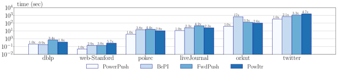
Figure 4. running time v.s. datasets, where the number $c.c\times$ over each bar means $c.c$ times of PowerPush’s running time

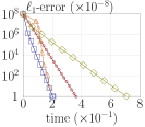
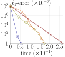
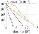
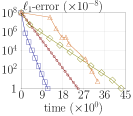
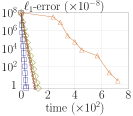
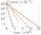
(a) dblp	(b) web-Stanford	(c) pokec	(d) liveJournal	(e) orkut	(f) twitter

Figure 5. actual $\ell_{1}$-error v.s. execution time (seconds)

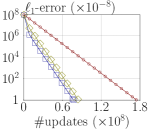
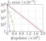
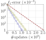
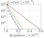
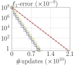
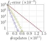
(a) dblp	(b) web-Stanford	(c) pokec	(d) liveJournal	(e) orkut	(f) twitter

Figure 6. actual $\ell_{1}$-error v.s. #residue updates

8. Experiments

In this section, we evaluate our proposed algorithms and verify our theoretical analysis with experiments.

Datasets. We use six real datasets: DBLP (Yang and Leskovec, 2012), Web Stanford (Web-St) (Leskovec et al., 2009), Pokec (Takac and Zábovský, 2012), Live Journal (LJ) (Backstrom et al., 2006), Orkut (Yang and Leskovec, 2012), and Twitter (Kwak et al., 2010). These datasets have been commonly used in the experiments in the previous work (Wang et al., 2016, 2017; Wei et al., 2018; Lin et al., 2020; Lofgren et al., 2016), on which the algorithm performance are considered as benchmarks. While the graphs in DBLP and Orkut are un-directed, we replace each un-directed edge with two directed edges in both directions. For each dataset, we remove the isolated nodes, i.e., the nodes have no in-coming nor out-going edges; for the rest nodes, we relabel their id’s with integers starting from $0$. Table 1 shows the statistics of the datasets after the above cleaning process. Finally, in the experiments for evaluating the query efficiency, for each dataset, we perform queries on $30$ query source nodes generated uniformly at random for all the competitors and take the average query time.

Dataset	Index Size			Construction Time
	High-Prec.	Approx.		High-Prec.	Approx.
	BePI	FORA	SpeedPPR	BePI	FORA	SpeedPPR
DBLP	23.9MB	139MB	8.01MB	1.72	6.53	0.520
Web-St	31.7MB	137MB	8.82MB	1.92	4.21	0.489
Pokec	1.13GB	1.24GB	118MB	75.4	248	16.2
LJ	2.32GB	3.31GB	263MB	185	612	38.8
Orkut	54.5GB	4.80GB	894MB	57988	1410	173
Twitter	24.5GB	47.8GB	5.48GB	6180	19883	1256

Table 2. Index Size and Construction Time (in seconds)

Competitors. There are two groups of competitors respectively for the experiments on high-precision and approximate SSPPR queries. For the high-precision queries, we have the four competitors: PowItr, FIFO-FwdPush, PowerPush and BePI (Jung et al., 2017): a state-of-the-art high-precision SSPPR algorithm which was reported that it outperforms most of (if not all) other existing works. For the approximate queries, we compare the performance of the following competitors: SpeedPPR, SpeedPPR-Index, FORA (Wang et al., 2019), FORA-Index (Wang et al., 2019), and ResAcc (Lin et al., 2020): a most recent approximate SSPPR algorithm which was reported to have competitive performance comparing to FORA.

Experiment Environment. All the experiments are conducted on a cloud based Linux 20.04 server with Intel 2.0 GHz CPU and 144GB memory. Except BePI, all the competitors are implemented with C++, where the source code of the implementations of our algorithms can be found at here and the implementations of FORA, FORA-Index and ResAcc are open-source and provided by their respective authors. Since only the MATLAB P-code of BePI is released, we can only run BePI as a black box. All the C++ implementations are complied with GCC 9.3.0 with -O3 optimization.

8.1. Evaluations of High-Precision SSPPR

In this experiment, we evaluate the high-precision SSPPR algorithms. For PowItr, FIFO-FwdPush and PowerPush, we set the $\ell_{1}$-error threshold $\lambda=\min\{10^{-8},1/m\}$. BePI adopts a different error measurement, which is to compute the $\ell_{2}$ distance between the obtained results in two consecutive iterations, namely, $\|\hat{\pi_{s}}^{(j+1)}-\hat{\pi_{s}}^{(j)}\|_{2}=\sqrt{\sum_{v\in V}\left(\hat{\pi}^{(j+1)}(s,v)-\hat{\pi}^{(j)}(s,v))\right)^{2}}$; when this $\ell_{2}$ distance is no more than a specified convergence parameter $\Delta$, it considers the current result $\hat{\pi_{s}}^{(j+1)}$ converges and thus stops. For BePI, we set $\Delta=\min\{10^{-8},1/m\}$. It should be noted that under this setting of $\Delta$, the results obtained by BePI do not necessarily meet the requirement that the $\ell_{1}$-error (with respect to the ground truth $\vec{\pi_{s}}$) is at most $\lambda$. Therefore, its running time reported in the following experiments is an underestimate of BePI’s actual time to achieve the $\ell_{1}$-error $\lambda$.

Moreover, among all these four competitors, BePI is the only one that requires pre-computed index. Table 2 shows the pre-processing time and the index space consumption of BePI . BePI takes $57,988$ seconds (over $15$ hours) to compute the index on Orkut and $6,180$ seconds on Twitter, which consume $54.5$GB and $24.5$GB space, respectively. This is because BePI is a matrix-based algorithm and thus affected heavily by the density of the graph. As shown in Table 1, the average degree of Orkut is $76.3$ while the one of Twitter is $35.3$. Hence, the pre-processing time (rsp. index size) of the former is significantly longer (rsp. larger) than that of the latter.

Average Overall Query Time. Figure 4 reports the average overall running time of all the algorithms for the randomly generated query source nodes over all the datasets. The running time of PowerPush is the smallest on all datasets except DBLP, the dataset with fewest edges among the six, where PowerPush is slightly worse than BePI. It is worth pointing out that even taking the advantages of a significant pre-processing (whose cost is not counted in the query time), BePI is still $2\times$ to $4\times$ slower than our PowerPush in general. In particular, on Orkut, PowerPush is $17\times$ faster than BePI even without any pre-processing or index. This shows a significant superiority of PowerPush over BePI. On the other hand, FIFO-FwdPush and PowItr have similar performance over all the datasets. This is reasonable because they are essentially equivalent and having the same time complexity. Interestingly, as PowerPush is carefully designed to incorporate both the strengths of PowItr and FIFO-FwdPush, PowerPush outperforms both of them in all cases.

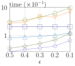
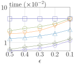
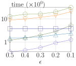
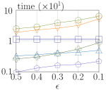
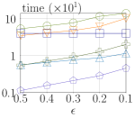
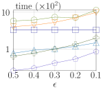
(a) dblp	(b) web-Standford	(c) pokec	(d) liveJournal	(e) orkut	(f) twitter

Figure 7. running time (seconds) v.s. $\epsilon$

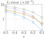
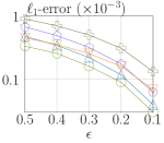
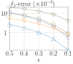
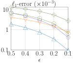
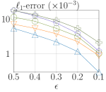
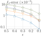
(a) dblp	(b) web-Standford	(c) pokec	(d) liveJournal	(e) orkut	(f) twitter

Figure 8. actual $\ell_{1}$-error v.s. $\epsilon$

Actual $\ell_{1}$-Error v.s. Execution Time. Figure 5 shows the actual $\ell_{1}$-error $r_{\text{sum}}$ (in log scale) versus the execution time of all the competitors. In this experiment, we take the query that incurs the median running time (among the 30 queries) of PowerPush on each dataset as reference. Each of these diagrams is plotted based on the execution with the corresponding median query source node. Except BePI, the data points in the diagrams of each algorithm are plotted for the moments of every $4\cdot m$ edge pushing’s (where each push operation on $v$ is counted as $d_{v}$ edge pushing’s). As BePI adopts different error measurement, we take a decreasing sequence of $\Delta$ values until $\Delta=\min\{1/m,10^{-8}\}$ for BePI and compute the corresponding $\ell_{1}$-error for the obtained results, and plot these $\ell_{1}$-errors along with the corresponding execution time. In the diagrams, some curves of BePI do not touch the bottom; in these cases, BePI did not manage to obtain an estimation within $\ell_{1}$-error $\lambda$ under the corresponding parameter setting.

There are three crucial observations from Figure 5. First, PowerPush has the fastest convergence speed on all datasets, where it outperforms BePI by (i) an order of magnitude on Orkut, (ii) roughly two to four times on the other datasets except DBLP, and (iii) having roughly the same running time on DBLP. This is consistent with our observation from Figure 4. Second, except BePI, the curves of the other three algorithms are pretty straight with the log-scale y-axis. This implies that their $\ell_{1}$-errors decrease in an exponential speed with running time, and thus it matches their $O(m\cdot\log\frac{1}{\lambda})$ time complexity. Third, PowItr has a faster convergence speed than FIFO-FwdPush on four out of six datasets. This is a bit counter-intuitive at the first glance. But the reason for this is that after a few iterations, there would be a large number of active nodes. In this case, the global sequential scan performs better than the random access in FIFO-FwdPush. This shows the importance of combining the global and local approach in PowerPush.

Actual $\ell_{1}$-Error v.s. # of Residue Updates. We further investigate the effectiveness of the push operations in the algorithms. Figure 6 demonstrates the $\ell_{1}$-error (in log scale) with respect to the number of edge pushing’s, that is the number of residue updates. Note that BePI is not applicable to this experiment, as we have no access to the operation number during its execution. Except the first few updates, the log-scale $\ell_{1}$-errors of both FIFO-FwdPush and PowerPush decreases linearly. This complies with our theoretical analysis. As expected, the pushes of FIFO-FwdPush are more effective than those in PowItr, because they are performed in an asynchronous manner. Among the three algorithms, the proposed PowerPush requires the least number of residue updates (to achieve the same $\ell_{1}$-error) in most datasets. This is because the dynamic threshold optimization enables PowerPush to “accumulate” the residues of the nodes before pushing. And thus, it further reduces the number of the push operations. Of interest is Orkut, in which PowerPush performs similar number of updates as FIFO-FwdPush. However, as shown in Figure 5, PowerPush requires much less time than FIFO-FwdPush on the same dataset. The reason is that the global sequential scan technique makes the memory access pattern in PowerPush more cache-friendly and hence more efficient to perform pushes. Similar observation can also be found in the comparison between PowItr and FIFO-FwdPush on Orkut, where PowItr performs a much larger number of operations but it achieves a similar execution time as FIFO-FwdPush’s.

8.2. Evaluations of Approximate SSPPR

Next, we evaluate the approximate SSPPR algorithms against different $\epsilon$ values from $0.1$ to $0.5$, and report their running time as well as the solution quality in terms of $\ell_{1}$-error. For the index version of FORA, we generate its index with the smallest $\epsilon$ in consideration, i.e., $\epsilon=0.1$, and re-use it for other $\epsilon$’s. For the index-based SpeedPPR, its index size does not depend on $\epsilon$. As shown in Table 2, SpeedPPR outperforms FORA in both pre-processing time and index size by an order of magnitude.

Running Time v.s. $\epsilon$. Figure 7 shows the running time (in log scale) of all the competitors over the six datasets. Note that we deliberately include our high-precision algorithm PowerPush in these diagrams as a base line. Interestingly, it shows comparable or even better performance comparing to the state-of-the-art index-free approximate algorithms (FORA and ResAcc) on some datasets. Furthermore, observe that SpeedPPR-Index demonstrates superior performance over all datasets. The index-free version of SpeedPPR is slightly slower than FORA-Index. Indeed, except for the two smallest datasets, the efficiency of SpeedPPR is comparable or even better than that of FORA-Index with small $\epsilon$’s. Both SpeedPPR and SpeedPPR-Index show a linear increase on the running time (in log scale), especially on Orkut and Twitter.

Actual $\ell_{1}$-Error v.s. $\epsilon$. Finally, we study the solution quality of the approximate algorithms. Figure 8 shows the $\ell_{1}$-error with respect to the ground truth $\vec{\pi_{s}}$ which is computed with PowerPush by setting $\lambda=10^{-17}$, the highest possible precision for the data type double in C++. Except on the dataset web-Stanford, SpeedPPR offers the best solution quality. When $\epsilon$ is small, its solution quality could be an order of magnitude better than other algorithms. This is impressive, considering it just takes comparable running time of FORA-Index. Another observation is that both SpeedPPR-Index and FORA-Index provide inferior solutions compared to the index-free algorithms. The reason for this is that the index-based algorithms tend to use more random walks as the walks can be performed with a relatively small cost. These algorithms thus spend less time on the local push phase, which actually computes the estimation deterministically. As a result, the random walks are performed based on a larger $r_{\text{sum}}$ leading to a larger variance in the estimations.

9. Conclusion

In this paper, we show an equivalent connection between the two fundamental algorithms PowItr and FwdPush. Embarking from this connection, we further prove that the time complexity of a common FwdPush implementation is $O(m\cdot\log\frac{1}{\lambda})$, where $\lambda$ is the $\ell_{1}$-error threshold. This answers the long-standing open question regarding the time complexity of FwdPush in the dependency on $\lambda$. Based on this finding, we propose a new implementation of PowItr, called PowerPush, which incorporates both the strengths of PowItr and FwdPush. Furthermore, we propose a new algorithm, called SpeedPPR for answering approximate single-source PPR queries. The expected time complexity of SpeedPPR is $O(n\log n\log\frac{1}{\epsilon})$ on scale-free graphs, improving the state-of-the-art $O(\frac{n\log n}{\epsilon})$-bound. In addition, SpeedPPR admits an index with size always at most $O(m)$ independent on $\epsilon$. Our experimental results show that our PowerPush and SpeedPPR outperform their state-of-the-art competitors by up to an order of magnitude in all evaluation metrics.

References

- (1)
- Andersen et al. (2007) Reid Andersen, Christian Borgs, Jennifer T. Chayes, John E. Hopcroft, Vahab S. Mirrokni, and Shang-Hua Teng. 2007. Local Computation of PageRank Contributions. In WAW. 150–165.
- Andersen et al. (2006) Reid Andersen, Fan R. K. Chung, and Kevin J. Lang. 2006. Local Graph Partitioning using PageRank Vectors. In FOCS. 475–486.
- Backstrom et al. (2006) Lars Backstrom, Daniel P. Huttenlocher, Jon M. Kleinberg, and Xiangyang Lan. 2006. Group formation in large social networks: membership, growth, and evolution. In Proceedings of the Twelfth ACM SIGKDD International Conference on Knowledge Discovery and Data Mining, Philadelphia, PA, USA, August 20-23, 2006, Tina Eliassi-Rad, Lyle H. Ungar, Mark Craven, and Dimitrios Gunopulos (Eds.). ACM, 44–54.
- Backstrom and Leskovec (2011) Lars Backstrom and Jure Leskovec. 2011. Supervised random walks: predicting and recommending links in social networks. In WSDM. 635–644.
- Bahmani et al. (2011) Bahman Bahmani, Kaushik Chakrabarti, and Dong Xin. 2011. Fast personalized PageRank on MapReduce. In SIGMOD. 973–984.
- Bahmani et al. (2010) Bahman Bahmani, Abdur Chowdhury, and Ashish Goel. 2010. Fast incremental and personalized pagerank. VLDB 4, 3 (2010), 173–184.
- Berkhin (2005) Pavel Berkhin. 2005. Survey: A Survey on PageRank Computing. Internet Math. 2, 1 (2005), 73–120.
- Chakrabarti (2007) Soumen Chakrabarti. 2007. Dynamic personalized pagerank in entity-relation graphs. In WWW. 571–580.
- Chung and Lu (2006) Fan Chung and Linyuan Lu. 2006. Concentration inequalities and martingale inequalities: a survey. Internet Math. 3, 1 (2006), 79–127.
- Coskun et al. (2016) Mustafa Coskun, Ananth Grama, and Mehmet Koyuturk. 2016. Efficient processing of network proximity queries via chebyshev acceleration. In KDD. 1515–1524.
- Fogaras et al. (2005) Dániel Fogaras, Balázs Rácz, Károly Csalogány, and Tamás Sarlós. 2005. Towards scaling fully personalized pagerank: Algorithms, lower bounds, and experiments. Internet Mathematics 2, 3 (2005), 333–358.
- Fujiwara et al. (2012a) Yasuhiro Fujiwara, Makoto Nakatsuji, Makoto Onizuka, and Masaru Kitsuregawa. 2012a. Fast and Exact Top-k Search for Random Walk with Restart. PVLDB 5, 5 (2012), 442–453.
- Fujiwara et al. (2013a) Yasuhiro Fujiwara, Makoto Nakatsuji, Hiroaki Shiokawa, Takeshi Mishima, and Makoto Onizuka. 2013a. Efficient ad-hoc search for personalized PageRank. In SIGMOD. 445–456.
- Fujiwara et al. (2013b) Yasuhiro Fujiwara, Makoto Nakatsuji, Hiroaki Shiokawa, Takeshi Mishima, and Makoto Onizuka. 2013b. Fast and Exact Top-k Algorithm for PageRank. In AAAI.
- Fujiwara et al. (2012b) Yasuhiro Fujiwara, Makoto Nakatsuji, Takeshi Yamamuro, Hiroaki Shiokawa, and Makoto Onizuka. 2012b. Efficient personalized pagerank with accuracy assurance. In KDD. 15–23.
- Guo et al. (2017) Tao Guo, Xin Cao, Gao Cong, Jiaheng Lu, and Xuemin Lin. 2017. Distributed Algorithms on Exact Personalized PageRank. In SIGMOD. 479–494.
- Gupta et al. (2008) Manish S. Gupta, Amit Pathak, and Soumen Chakrabarti. 2008. Fast algorithms for top-k personalized pagerank queries. In WWW. 1225–1226.
- Jeh and Widom (2003) Glen Jeh and Jennifer Widom. 2003. Scaling personalized web search. In WWW. 271–279.
- Jung et al. (2017) Jinhong Jung, Namyong Park, Sael Lee, and U Kang. 2017. BePI: Fast and Memory-Efficient Method for Billion-Scale Random Walk with Restart. In SIGMOD. 789–804.
- Kwak et al. (2010) Haewoon Kwak, Changhyun Lee, Hosung Park, and Sue B. Moon. 2010. What is Twitter, a social network or a news media?. In Proceedings of the 19th International Conference on World Wide Web, WWW 2010, Raleigh, North Carolina, USA, April 26-30, 2010, Michael Rappa, Paul Jones, Juliana Freire, and Soumen Chakrabarti (Eds.). ACM, 591–600.
- Leskovec et al. (2009) Jure Leskovec, Kevin J. Lang, Anirban Dasgupta, and Michael W. Mahoney. 2009. Community Structure in Large Networks: Natural Cluster Sizes and the Absence of Large Well-Defined Clusters. Internet Math. 6, 1 (2009), 29–123.
- Lin et al. (2020) Dandan Lin, Raymond Chi-Wing Wong, Min Xie, and Victor Junqiu Wei. 2020. Index-Free Approach with Theoretical Guarantee for Efficient Random Walk with Restart Query. In 2020 IEEE 36th International Conference on Data Engineering (ICDE). IEEE, 913–924.
- Lofgren et al. (2015) Peter Lofgren, Siddhartha Banerjee, and Ashish Goel. 2015. Bidirectional PageRank Estimation: From Average-Case to Worst-Case. In WAW. 164–176.
- Lofgren et al. (2016) Peter Lofgren, Siddhartha Banerjee, and Ashish Goel. 2016. Personalized pagerank estimation and search: A bidirectional approach. In WSDM. 163–172.
- Lofgren et al. (2014) Peter A Lofgren, Siddhartha Banerjee, Ashish Goel, and C Seshadhri. 2014. Fast-ppr: Scaling personalized pagerank estimation for large graphs. In KDD. 1436–1445.
- Maehara et al. (2014) Takanori Maehara, Takuya Akiba, Yoichi Iwata, and Ken-ichi Kawarabayashi. 2014. Computing personalized PageRank quickly by exploiting graph structures. PVLDB 7, 12 (2014), 1023–1034.
- Ohsaka et al. (2015) Naoto Ohsaka, Takanori Maehara, and Ken-ichi Kawarabayashi. 2015. Efficient PageRank Tracking in Evolving Networks. In KDD. 875–884.
- Ou et al. (2016) Mingdong Ou, Peng Cui, Jian Pei, Ziwei Zhang, and Wenwu Zhu. 2016. Asymmetric Transitivity Preserving Graph Embedding. In Proceedings of the 22nd ACM SIGKDD International Conference on Knowledge Discovery and Data Mining, San Francisco, CA, USA, August 13-17, 2016, Balaji Krishnapuram, Mohak Shah, Alexander J. Smola, Charu C. Aggarwal, Dou Shen, and Rajeev Rastogi (Eds.). ACM, 1105–1114.
- Page et al. (1999) Lawrence Page, Sergey Brin, Rajeev Motwani, and Terry Winograd. 1999. The PageRank citation ranking: bringing order to the web. (1999).
- Ren et al. (2014) CH Ren, Luyi Mo, CM Kao, CK Cheng, and DWL Cheung. 2014. CLUDE: An Efficient Algorithm for LU Decomposition Over a Sequence of Evolving Graphs. In EDBT.
- Sarma et al. (2015) Atish Das Sarma, Anisur Rahaman Molla, Gopal Pandurangan, and Eli Upfal. 2015. Fast distributed pagerank computation. Theoretical Computer Science 561 (2015), 113–121.
- Shin et al. (2015) Kijung Shin, Jinhong Jung, Lee Sael, and U. Kang. 2015. BEAR: Block Elimination Approach for Random Walk with Restart on Large Graphs. In SIGMOD. 1571–1585.
- Takac and Zábovský (2012) L. Takac and Michal Zábovský. 2012. Data analysis in public social networks. International Scientific Conference and International Workshop Present Day Trends of Innovations (01 2012), 1–6.
- Tsitsulin et al. (2018) Anton Tsitsulin, Davide Mottin, Panagiotis Karras, and Emmanuel Müller. 2018. VERSE: Versatile Graph Embeddings from Similarity Measures. In Proceedings of the 2018 World Wide Web Conference on World Wide Web, WWW 2018, Lyon, France, April 23-27, 2018, Pierre-Antoine Champin, Fabien L. Gandon, Mounia Lalmas, and Panagiotis G. Ipeirotis (Eds.). ACM, 539–548.
- Wang et al. (2016) Sibo Wang, Youze Tang, Xiaokui Xiao, Yin Yang, and Zengxiang Li. 2016. HubPPR: Effective Indexing for Approximate Personalized PageRank. PVLDB 10, 3 (2016), 205–216.
- Wang et al. (2019) Sibo Wang, Renchi Yang, Runhui Wang, Xiaokui Xiao, Zhewei Wei, Wenqing Lin, Yin Yang, and Nan Tang. 2019. Efficient Algorithms for Approximate Single-Source Personalized PageRank Queries. ACM Trans. Database Syst. 44, 4 (2019), 18:1–18:37.
- Wang et al. (2017) Sibo Wang, Renchi Yang, Xiaokui Xiao, Zhewei Wei, and Yin Yang. 2017. FORA: Simple and Effective Approximate Single-Source Personalized PageRank. In KDD. 505–514.
- Wei et al. (2018) Zhewei Wei, Xiaodong He, Xiaokui Xiao, Sibo Wang, Shuo Shang, and Ji-Rong Wen. 2018. Topppr: top-k personalized pagerank queries with precision guarantees on large graphs. In Proceedings of the 2018 International Conference on Management of Data. 441–456.
- Wu et al. (2014) Yubao Wu, Ruoming Jin, and Xiang Zhang. 2014. Fast and unified local search for random walk based k-nearest-neighbor query in large graphs. In SIGMOD 2014. 1139–1150.
- Yang and Leskovec (2012) Jaewon Yang and Jure Leskovec. 2012. Defining and Evaluating Network Communities Based on Ground-Truth. In 12th IEEE International Conference on Data Mining, ICDM 2012, Brussels, Belgium, December 10-13, 2012, Mohammed Javeed Zaki, Arno Siebes, Jeffrey Xu Yu, Bart Goethals, Geoffrey I. Webb, and Xindong Wu (Eds.). IEEE Computer Society, 745–754.
- Yin and Wei (2019) Yuan Yin and Zhewei Wei. 2019. Scalable Graph Embeddings via Sparse Transpose Proximities. In Proceedings of the 25th ACM SIGKDD International Conference on Knowledge Discovery & Data Mining, KDD 2019, Anchorage, AK, USA, August 4-8, 2019, Ankur Teredesai, Vipin Kumar, Ying Li, Rómer Rosales, Evimaria Terzi, and George Karypis (Eds.). ACM, 1429–1437.
- Yu and Lin (2013) Weiren Yu and Xuemin Lin. 2013. IRWR: incremental random walk with restart. In SIGIR. 1017–1020.
- Yu and McCann (2016) Weiren Yu and Julie A. McCann. 2016. Random Walk with Restart over Dynamic Graphs. In ICDM. 589–598.
- Zhang et al. (2016) Hongyang Zhang, Peter Lofgren, and Ashish Goel. 2016. Approximate Personalized PageRank on Dynamic Graphs. In KDD. 1315–1324.
- Zhang et al. (2020) Kai Zhang, Yaokang Zhu, Jun Wang, and Jie Zhang. 2020. Adaptive Structural Fingerprints for Graph Attention Networks. In 8th International Conference on Learning Representations, ICLR 2020, Addis Ababa, Ethiopia, April 26-30, 2020. OpenReview.net.
- Zhu et al. (2013) Fanwei Zhu, Yuan Fang, Kevin Chen-Chuan Chang, and Jing Ying. 2013. Incremental and Accuracy-Aware Personalized PageRank through Scheduled Approximation. PVLDB 6, 6 (2013), 481–492.