White Dwarf Photospheric Abundances in Cataclysmic Variables:
I. SS Aurigae and TU Mensae

Abstract

Chemical abundances studies of cataclysmic variables have revealed high nitrogen to carbon ratios in a number of of cataclysmic variable white dwarfs (based on ultraviolet emission and absorption lines), as well as possible carbon deficiency in many secondaries (based on the absence of infrared CO absorption lines). These indicate that the accreted material on the white dwarf surface and the donor itself might be contaminated with CNO processed material. To further understand the origin of this abundance anomaly, there is a need for further chemical abundance study. In the present work, we carry out a far ultraviolet spectral analysis of the extreme SU UMa dwarf nova TU Men and the U Gem dwarf nova SS Aur using archival spectra. We derive the mass and temperature of the WD using the recently available DR2 Gaia parallaxes. The analysis of HST STIS spectra yields a WD mass $M_{\rm wd}=0.77^{+0.16}_{-0.13}M_{\odot}$ with a temperature of $27,750\pm 1000$ K for TU Men, and a WD mass $M_{\rm wd}\sim 0.80\pm 0.15$ with a temperature of $\sim 30,000\pm 1000$ K for SS Aur. However, the analysis of a FUSE spectrum for SS Aur gives to a higher temperature $\sim 33,375\pm 1875$ K, yielding to a higher WD mass $\sim 1\pm 0.25M_{\odot}$, which could be due to the effect of a second hot emitting component present in the short wavelengths of FUSE. Most importantly, based on the white dwarf far ultraviolet absorption lines, we find that both systems have subsolar carbon and silicon abundances. For TU Men we also find suprasolar nitrogen abundance, evidence of CNO processing.

Astroph Version 0.9in

1 Introduction

The study of cataclysmic variables (CVs) has focused primarily on deriving the system parameters (i.e. binary period, binary masses and temperatures, inclination, mass accretion rate,..) while less emphasis has been put on deriving the chemical abundances of the WD stellar photosphere. The main reason has been that to confront the theories of CVs evolution one primarily needs to know the binary period, the white dwarf (WD) mass, and the WD temperature or the mass accretion rate for a large number of systems (e.g. Pala et al., 2017). In addition, deriving stellar surface abundances demands a priori high quality spectra and meticulous phase-resolved spectral analysis, especially in the ultraviolet (UV; e.g. Long et al., 2006; Godon et al., 2017a). In spite of that, chemical abundances studies of CVs have revealed high nitrogen to carbon ratios in a dozen CV WDs based on UV N v/Civ emission line ratios (e.g. Gänsicke et al., 2003) and UV absorption lines (e.g. Sion et al., 1997, 1998; Long et al., 2009; Gänsicke et al., 2005), as well as possible carbon deficiency in many secondaries (based on the absence of infrared CO absorption lines, see Howell et al., 2010, for a short review). From the study of a limited sample of CVs, it is estimated that possibly up to 10-15% of all CVs might have anomalously high N/C ratio (Gänsicke et al., 2003). These results demonstrate the need for further studies to obtain stellar chemical abundances of the WD, the donor, and/or the disk.

In the present work, we present an analysis of the extreme SU UMa dwarf nova TU Men and the U Gem dwarf nova SS Aur as the first results of a much larger far-ultraviolet (FUV) analysis of CV systems to derive the chemical abundances in CV WDs. We chose these two systems as we previously analyzed them, they have relatively good spectra revealing the white dwarf and exhibiting absorption lines, and, as it appears a posteriori, they both show evidence of non-solar composition and possible CNO processed material.

For that purpose, we analyze the medium quality/resolution short exposure time Hubble Space Telescope (HST) Space Telescope Imaging Spectrograph (STIS) G140L/1425 snapshot spectra of TU Men and SS Aur. For SS Aur, we also analyze a Far Ultraviolet Spectroscopic Explorer (FUSE) spectrum. We improve on our previous analysis (Godon et al., 2008; Sion et al., 2008) of these two systems by considering a large range of values in the parameter space ($Log(g),T_{\rm wd}$), using the Gaia DR2 derived distances, and applying the reduced chi-squared statistic to find the best-fits. We further vary individual abundances of carbon, silicon, and nitrogen in the WD model atmosphere to assess the chemical abundances of the WD photospheres of these two systems. The STIS spectrum of TU Men reveals subsolar abundances of carbon and silicon as well as suprasolar abundance of nitrogen. The STIS spectrum of SS Aur too reveals subsolar abundances of carbon and silicon, as to its FUSE spectrum it only show signs of subsolar abundance of carbon.

We introduce the two systems in the next section and present the archival data in section 3. The details of our spectral analysis tools and technique are given in section 4. The results for the WD mass and temperature are presented in section 5 for both systems, while the results for the WD chemical abundances and projected stellar rotational (broadening) velocity are given in section 6. We conclude with a discussion in the last section.

Table 1: System Parameters

Parameter	Units	TU Men	SS Aur
Period	(d)	0.1172(1)	0.1828(6,7)
Inclination	(deg)	$44-70^{(1,5)}$	$38\pm 16^{(8)}$
Distance	(pc)	$278\pm 5^{(2)}$	$260\pm 3^{(2)}$
$E(B-V)$		$0.08\pm 0.02^{(4)}$	$0.08\pm 0.02^{(3)}$
WD Mass	$(M_{\odot})$	$0.6-1.06^{(1,5)}$	$1.08\pm 0.40^{(8)}$
$K_{1}$	(km/s)	$85-150^{(1,5)}$	$70\pm 10^{(6)}$

Note. — (1) Mennickent (1995); (2) derived from the Gaia DR2 parallax, Ramsay et al. (2017); Lindergren et al. (2018); Luri et al. (2018); (3) Bruch & Engel (1994); (4) Godon et al. (2017b); (5) Stolz & Schoembs (1984); (6) Shafter & Harkness (1986); (7) Kraft & Luyten (1965); (8) Shafter (1983).

2 The Two Systems

TU Mensae.

TU Men is a peculiar SU UMa system exhibiting some rather extreme characteristics: it is the first SU UMa system discovered in the period gap with a period of $2^{h}.813$ (Mennickent, 1995); it has superoutburst maxima lasting for more than 20 days or longer, occurring at extremely long intervals ($\sim years$, Bateson et al., 2000); its disk is bright enough to induce emission on the surface of the secondary star (or alternatively it is the only SU UMa system to show emission from the secondary in quiescence, Tappert et al., 2003); and, with a mass ratio $\sim 0.5\pm 0.2$, it belongs to a category of systems exhibiting superhumps in spite of their longer orbital periods and higher mass ratios ($q>q_{crit}=0.25$, Smak, 2006).

Its WD mass is unknown and estimates varies from $\sim 0.6M_{\odot}$ (Stolz & Schoembs, 1984), $0.785\pm 0.145M_{\odot}$ to possibly $\approx 1.06M_{\odot}$ (Mennickent, 1995). Its $K_{1}$ amplitude was first measured from absorption lines in outburst and found to be $\approx$150 km/s (Stolz & Schoembs, 1984), while a measure from the emission lines at quiescence gave $K_{1}=108\pm 10$ km/s or possibly $K_{1}=87\pm 2$ km/s (Mennickent, 1995). These yielded, respectively, a mass ratio of q=0.59, 0.455, and 0.33, all larger than the critical value of 0.25, below which the observed superhumps are believed to be due to the tidal instability of the 3:1 resonance. It was shown (Smak, 2006) that numerical simulations, on which the $q<0.25$ criterion was based, do not apply to the observed superhumps. Its inclination is possibly moderate and estimates have put it at $65^{\circ}\pm 10^{\circ}$ (Stolz & Schoembs, 1984), $52^{\circ}\pm 2^{\circ}$ or even as low as $\approx 44^{\circ}$ (Mennickent, 1995). Well before Gaia, its distance was estimated to be 270 pc by fitting the observed Balmer absorption lines to theoretical accretion disk lines for a mass transfer rate $\dot{M}=6\times 10^{17}$g s^-1, a white dwarf mass $M_{\rm wd}=0.6M_{\odot}$, $q=0.588$, and $i=65^{\circ}$ (Stolz & Schoembs, 1984). This is remarkably close to its Gaia DR2 derived distance of $278\pm 5$ pc, in spite of the fact the mass might be significantly larger, with a smaller inclination and mass ratio.

SS Aurigae.

SS Aur is a fairly normal U Gem type dwarf nova with a period of $4^{h}.3872$ (Kraft & Luyten, 1965; Shafter & Harkness, 1986). The amplitude of the WD velocity, inferred from the variation of the H_α emission lines, is $70\pm 10$ km/s (Shafter & Harkness, 1986). The systems parameters were obtained by Shafter (1983), but with a rather larger error for the WD mass ($1.08\pm 0.40M_{\odot}$) and inclination ($i=38\pm 16^{\circ}$).

A HST fine guidance sensors (FGS) parallax was obtained for SS Aur, which, after calibration and correction, gave $4.97\pm 0.65$ mas (Harrison et al., 2000), or a distance of $201^{+30}_{-23}$ pc. However, the DR2 Gaia parallax of $3.849\pm 0.041$ mas (Ramsay et al., 2017; Lindergren et al., 2018; Luri et al., 2018) gives a distance of $260\pm 3$ pc, which we adopt here.

While many non-magnetic CVs show possible carbon deficiency in their secondaries, based on the absence or weakness of infrared CO absorption lines, SS Aur is one of a few DNe presenting normal IR CO absorption lines (Howell et al., 2010).

The parameters of both systems are presented in Table 1 with their source references.

3 The Archival Data

TU Men was observed with HST STIS on Jan 03, 2003, about 10 days after the end of an outburst. The STIS instrument was set up in the FUV configuration with the G140L grating centered at 1425 Å (with the 52”x0.2” aperture), thereby producing a spectrum from $\sim$1140 Å to $\sim$1715 Å  (with a spectral resolution of $R\sim 1000$). The data (O6LI56010) were collected in ACCUM mode and consist in one echelle spectrum only with a total good exposure time of 900 s.

SS Aur was observed with HST STIS on Mar 20, 2003, as part of the same “snapshot survey” as TU Men (Gänsicke et al., 2003; Sion et al., 2008), with the STIS instrument set up exactly in the same configuration. The data (O6LI0F010) were collected more than a year after the FUSE observations (see below), and 36 days after an outburst, totaling 600 s of good exposure time.

All the HST STIS data were processed through the pipeline with CALSTIS version 2.13b. The STIS spectra of TU Men and SS Aur were presented in Sion et al. (2008) and Godon et al. (2008), respectively, with line identification.

We also used recently retrieved data processed with CALSTIS version 3.4.2, and extracted new spectra. We compare them to the data processed with CALSTIS version 2.13b (Godon et al., 2008; Sion et al., 2008) and found a very small change in the continuum flux level reaching a maximum of 3%. This is of the same amplitude as the systematic errors from instrument calibration $\sim 3$%. For comparison, the uncertainty in E(B-V) ($0.08\pm 0.02$; see below) produces a change of 18% in the continuum flux level (see also Results Section 5).

SS Aur was observed with FUSE on Feb 13, 2002 (Sion et al., 2004), at quiescence, 28 days after an outburst. The first dataset has an exposure time of $\sim$800 s, followed by 5 more data sets (obtained during successive FUSE orbits) with an exposure time nearing $\sim 2400$ s each, totaling 12,733 s of good exposure time. The data were collected through the LWRS aperture in time tag (TTAG) mode, and processed through the pipelines with the final version of CalFUSE (v3.2.3; van Dixon et al., 2007).

The FUSE spectrum requires special attention, as the data come in the form of eight spectral segments which are combined together to give the final FUSE spectrum. The spectral segments were individually examined (Godon et al., 2008, by visual inspection) to remove low-sensitivity portions, as well as other instrument artifacts (such as the “worm”) that cannot be corrected by CalFUSE (due to unpredicted temporal changes in strength and position of the artifact, Moos et al., 2000; Sahnow et al., 2000; van Dixon et al., 2007). Further details on the processing of the FUSE spectrum of SS Aur were given in Godon et al. (2012).

Table 2: Archival Data Observation Log

System	Instrument	Configuration	DATA ID	Date (UT)	Time (UT)	Exp.time	Fig.	Time since
Name				YYYY Mon DD	hh:mm:ss	sec	#	outburst
TU Men	HST STIS/FUV	G140L (1425)	O6LI56010	2003 Jan 04	01:47:53	900	1,8,10,11	10 d
SS Aur	HST STIS/FUV	G140L (1425)	O6LI0F010	2003 Mar 20	11:39:59	600	5,12	36 d
	FUSE	LWRS	C11002010	2002 Feb 13	06:49:53	12733	7,13	28 d

Note. — The date/time refer to the start of the observation, the exposure time is the total good exposure time.

The FUSE spectra are subject to larger systematic errors than the STIS spectra, with an uncertainty in the FUSE flux calibration estimated at $\sim$10-15% (FUSE data handbook v1.1). More specifically, data that were obtained early in the mission (as is the case for SS Aur) might suffer from a measured flux that is too high by 5-10% in the LiF2A channel (1095-1135 Å), and the LiF1B channel (covering about the same wavelength as the LiF2A) can be off by up to 10% (FUSE DATA Handbook 2009). An explicit comparison of the same FUV sources (Bohlin et al., 2014) shows that FUSE spectra exhibit a local flux variation of $\pm 5$% compared to STIS spectra. We can, therefore, assume a systematic error of at least $\sim 10\%$ in the continuum flux level for FUSE, and possibly as high as $\sim 15\%$.

With a wavelength coverage from $\sim 905$ Å to $\sim 1095$ Å, the FUSE telescope was the ideal instruments to study the hot accreting WDs in CVs. However, FUSE spectra are often contaminated with interstellar medium (ISM) absorption lines dominated by atomic and molecular hydrogen lines (e.g. Sembach, 2001), as the Lyman series extends from $\sim 912$ Å to 1216 Å . Because of its location near the galactic plane, and in spite of it being only at 260 pc, SS Aur presents some prominent ISM absorption lines in its FUSE spectrum. Explicitly, these lines consist in the W-Wener and L-Lyman band, upper vibrational level (1-16), and rotational transition (R,P, or Q with lower rotational state J=1-3). Additional ISM lines include lines from N i & N ii, Fe ii, Si ii, and C ii. The ISM absorption lines in the FUSE spectrum of SS Aur were identified in Godon et al. (2008).

The observation log of both the FUSE and HST archival data is presented in Table 2.

In preparation for the fitting, we deredden the spectra assuming E(B-V)=0.08 (see Table 1). For the extinction curve, we use the analytical expression of Fitzpatrick & Massa (2007), that we have slightly modified to agree with an extrapolation of Savage & Mathis (1979) in the FUSE range. Sasseen et al. (2002) have shown (see also Selvelli & Gilmozzi, 2013) that in the FUV range the observed extinction curve is actually consistent with an extrapolation of the standard extinction curve of Savage & Mathis (1979). For many CVs the reddening value has been estimated by “ironing out” the 2175 Å extinction bump (e.g. Verbunt, 1987, using International Ultraviolet Explorer (IUE) spectra). However, the normalized height of the 2175 Å feature has an accuracy of about $\pm 20$% and it has been suggested (Fitzpatrick, 1999) that, as a consequence, the uncertainty in $E(B-V)$ (derived from ironing out the bump) must have a similar relative uncertainty. In the present case we assume an uncertainty of $\pm 0.02$ for a reddening $E(B-V)=0.08$ (the two systems have the same value), or $\pm 25$%.

4 FUV Spectral Analysis Tools and Technique

We use the suite of codes TLUSTY/SYNSPEC (Hubeny, 1988; Hubeny & Lanz, 1995) to generate synthetic spectra for high-gravity stellar atmosphere WD models. A one-dimensional vertical stellar atmosphere structure is first generated with TLUSTY for a given surface gravity ($Log(g)$), effective surface temperature ($T_{\rm wd}$), and surface composition. Subsequently, the code SYNSPEC is run, using the output from TLUSTY as an input, to solve for the radiation field and generate a synthetic stellar spectrum over a given wavelength range between 900 Å and 7500 Å. The code includes the treatment of the quasi-molecular satellite lines of hydrogen which are often observed as a depression around 1400 Å and around 1060 Å and 1080 Å in the STIS and FUSE spectra (respectively) of WDs at low temperatures and high gravity: $T_{\rm wd}\leq 30,000$ K and $Log(g)\geq 7.50$, (e.g. see Godon et al., 2008). For temperatures above 35,000 K, we switch on the NLTE option with lines, considering all lines of H and He explicitly. Last, the code ROTIN is used to reproduce rotational and instrumental broadening as well as limb darkening. Technical and practical details on the suite of codes TLUSTY/SYNSPEC are given in Hubeny & Lanz (2017a, b, c), and the FORTRAN programs (with input files and examples) are downloadable from the TLUSTY webpage.

In this manner we have already generated solar composition stellar photospheric spectra covering a wide range of effective temperatures $T_{\rm wd}$ and surface gravities $Log(g)$: from $\sim$18,000 K to $\sim$40,000 K in steps of 1000 K, and an effective surface gravity from $Log(g)=7.0$ to $Log(g)=9.0$ in steps of 0.2. For each WD temperature and gravity there is a single WD radius $R_{\rm wd}$ and mass $M_{\rm wd}$, obtained using the non-zero temperature C-O WD mass-radius relation from Wood (1995).

The fitting of the observed spectra with theoretical spectra is carried out in two distinct steps: (i) in the first step we derive the WD effective surface temperature and gravity by fitting the continuum and the hydrogen Ly$\alpha$ profile; (ii) in the second step we derive the stellar surface abundances and the projected stellar rotational velocity by fitting the metal absorption lines.

4.1 Fitting the Continuum and Hydrogen Ly$\alpha$ Profile.

Using our existing theoretical model spectra with solar composition and a standard projected rotational velocity of $\sim$200 km/s for TU Men (which is common for cataclysmic variables) and $\sim$400 km/s for SS Aur (Godon et al., 2008; Sion et al., 2008), we fit the observed spectra using the $\chi^{2}_{\nu}$ minimization technique to find the best fit. Since we fit the continuum and the Lyman orders profile, the exact value of the velocity broadening (here the projected rotational velocity) does not affect the results. The correct value of the velocity is found in the second step together with the chemical abundance of the elements. The distance $d$ is also obtained for each model by scaling the model to the observed spectrum. Doing so we obtain the reduced $\chi^{2}_{\nu}$ ($\chi^{2}$ per degree of freedom $\nu$) and $d$ in the $T_{\rm wd}$ vs. $Log(g)$ parameter space. A preliminary check shows that for both TU Men and SS Aur, the least $\chi^{2}$ solutions for the known Gaia distance are obtained for $Log(g)>7.5$, and for a temperature of 25,000-35,000 K. We also find that the observed spectra are better fitted without the inclusion of the hydrogen quasi-molecular satellite line.

We, therefore, refine the grid of models and generate additional theoretical spectra, without the inclusion of the hydrogen quasi-molecular satellite lines, in the parameter space $(Log(g),T_{\rm wd})$: for $7.4\leq Log(g)\leq 9.0$, in steps of 0.1 in $Log(g)$, and for 23,000 K $\leq T_{\rm wd}\leq$ 37,000 K, in steps of 500 K in $T_{\rm wd}$. The refined grid consists of a total of 493 ($17\times 29$) solar composition theoretical WD spectra. We then carry out a new spectral to fit the observed spectra to obtain the least $\chi^{2}_{\nu}$ solutions in the two-dimensional parameter space $T_{\rm wd}$ vs $Log(g)$.

4.2 The $\chi^{2}$ Minimization Procedure and The Statistical Errors

We use a standard least-squares minimization approach to find the best-fit model and derive $T_{\rm wd}$ and $Log(g)$. In theory a good fit is obtained for a (reduced) chi-square $\chi^{2}_{\nu}\sim 1$, though in practice the least $\chi^{2}_{\nu~{}MIN}$ value can be smaller or larger than one. The value of $\chi^{2}$ is also subject to noise, which is inherited from the noise of the data. As a consequence there is an uncertainty in $\chi^{2}$ (and therefore $\chi^{2}_{\rm MIN}$), which translates into uncertainties on the derived parameters $Log(g)$ and $T_{\rm wd}$ - the statistical errors. For a number $p$ of parameters (here $p=2$, for $T_{\rm wd}$ and $Log(g)$), the uncertainty on the parameters $p$ is obtained for $\chi^{2}$ within the range $\chi^{2}_{\rm MIN}+\chi^{2}_{p}(\alpha)$, where $\chi^{2}_{p}(\alpha)$ is given in Table 3 for a significance $\alpha$, or equivalently, for a confidence $C=1-\alpha$ (see e.g. Lampton et al., 1976; Avni, 1976).

Table 3: Uncertainty in $\chi^{2}$ with $p$ Parameters and Significance $\alpha$ with $\nu$ Degrees of Freedom

Significance	Confidence	$\chi^{2}_{p}(\alpha)$
$\alpha$	C	$p=1$	$p=2$	$p=3$
0.32	0.68 (1.0$\sigma$)	1.00	2.30	3.50
0.10	0.90 (1.6$\sigma$)	2.71	4.61	6.25
0.01	0.99 (2.6$\sigma$)	6.63	9.21	11.3

Note. — If the data consist of $N$ data points to be fitted, and there are $p$ independent parameters, one has $\nu=N-p$. The uncertainty in the reduced chi square $\chi^{2}_{\nu}$ is obtained by dividing $\chi^{2}_{p}(\alpha)$ by the number of degrees of freedom $\nu$.

In the present work we derive the statistical errors on the best fit $T_{\rm wd}$ and $Log(g)$ for a 99% (2.6 $\sigma$) confidence level. The $p=2$ case is to be used when finding the error on the best-fit model in the two-dimensional parameter space $(T_{\rm wd},Log(g))$. However, as soon as one uses the known distance $d$ as a constraint, the problem is reduced to a one-parameter problem: one has to find the best fit along the line $distance=d$ in the $(T_{\rm wd},Log(g))$ parameter space. In that case one uses the $p=1$ case. We will come back to this in the result section.

4.3 Fitting the Metal Absorption Lines.

In the second step, after we found the best $Log(g)$ and $T_{\rm wd}$ fit for each spectrum, we vary the abundances of the elements Si, S, C, & N, one at a time, and vary the projected stellar rotational velocity, $V_{\rm rot}sin(i)$ in the best fit model. The abundances are varied from $0.01\times$ solar to $50\times$ solar in steps of about a factor of two or so; the projected stellar rotational velocity is varied from 50 km/s to 1000 km/ in steps of 50 km/s. The results of the abundances/velocity are then examined by visual inspection of the fitting of the absorption lines for each element. The reason we use visual examination rather than the $\chi^{2}$ minimization technique is that a visual examination can recognize and distinguish real absorption features from the noise, as the data quality is modest. This is partly because the spectral binning size ($\sim 0.58$ Å for STIS) is of the same order of magnitude as the width of some of the absorption lines, and the depth of some of the absorption features is of the amplitude as the flux errors. This is explicitly shown in Figs. 8 & 9 in the Results section 6. Details on our technique to derive stellar abundances and broadening velocities are also given in Godon et al. (2017a).

5 The White Dwarf Surface Temperature and Gravity.

5.1 TU Men

We first present the results for the WD temperature and gravity obtained from the spectral fit to the STIS spectrum of TU Men dereddened assuming $E(B-V)-=0.08$. Before the fitting we mask all the emission lines (including the Si iv doublet), the bottom of the Ly$\alpha$, as well as the absorption lines (such as e.g. the C iii 1175 Å, Si $\sim$ 1300 Å feature) since these depends on the exact abundances. We also mask a portion of the left wing of the Ly$\alpha$ as this region presents a possible emission region (near 1200 Å). We must stress that the masking of these spectral regions helps decrease the minimum $\chi^{2}_{\nu}$ (best fit) to a value close to 1. The best-fit model (Fig.1, with the masked regions in blue) has an effective surface gravity of $Log(g)=8.25\pm 0.25$, with an effective surface temperature of $27,750\pm 1000$ K. The model has a carbon abundance $[C]=0.2\pm 0.1$, silicon abundance $[Si]=0.2\pm 0.1$, and nitrogen abundance $[N]=20\pm 10$, all in solar abundance units (sun=1). The projected stellar rotational velocity of the model is $V_{rot}\sin(i)=225\pm 75$ km/s.

In the next paragraphs give a full account of how the best-fit model was obtained together with estimates of the systematic and statistical errors.

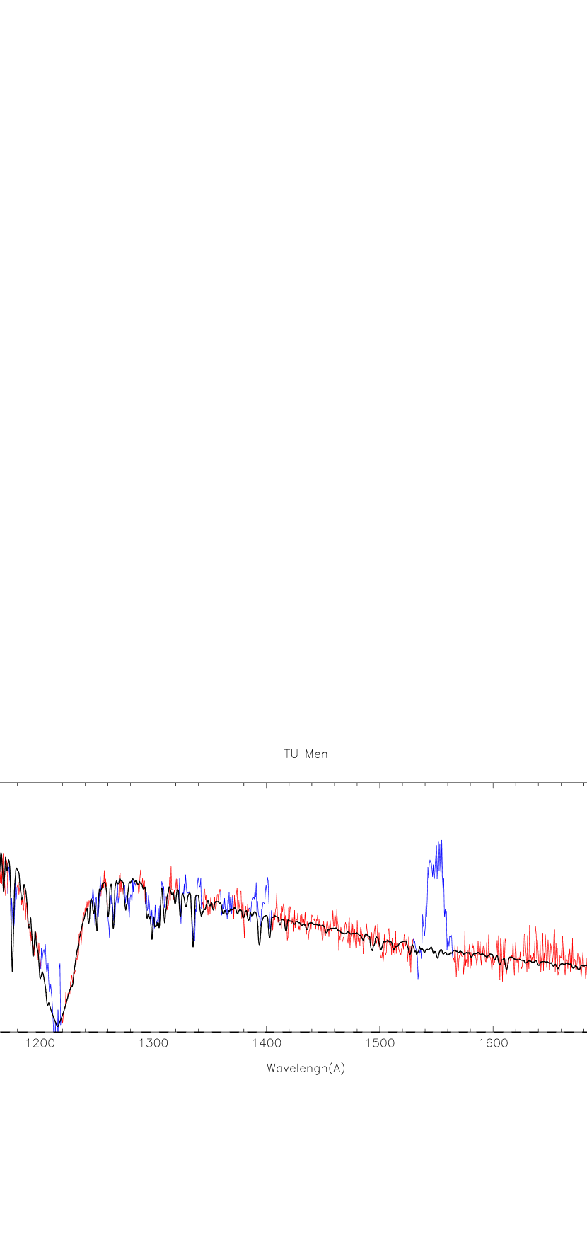
Figure 1: Modeling of the WD in TU Men. The HST STIS FUV spectrum of TU Men (in red) is fitted with a synthetic stellar spectrum (in black). The STIS spectrum has been dereddened assuming $E(B-V)=0.08$. A first fit is carried out where the emission lines and absorption lines are masked to find the temperature and gravity, these regions are in blue. Once the best-fit temperature and gravity are found, the absorption lines are fitted to find the abundances and projected rotational velocity. The WD model has an effective surface gravity of $Log(g)=8.25\pm 0.25$, with an effective surface temperature of $27,750\pm 1000$ K. The model has a carbon abundance $[C]=0.2\pm 0.1$, silicon abundance $[Si]=0.2\pm 0.1$, and nitrogen abundance $[N]=20\pm 10$, all in solar abundance units (sun=1). The projected stellar rotational velocity of the model is $V_{rot}\sin(i)=225\pm 75$ km/s.

The overall results are summarized in Fig.2, which were obtained using the refined grid of models (Sec.4). On the left panel we draw a grayscale of the $\chi^{2}_{\nu}$ value in the parameter space $(Log(g),T_{\rm wd})$. The least $\chi^{2}_{\nu}$ values (best fit models, in different shades of gray) form a diagonal starting at 25,000 K (for $Log(g)=7.5$) and extending to 30,500 K (for $Log(g)=9.0$). These models have $\chi^{2}_{\nu{\rm MIN}}\leq\chi^{2}_{\nu}\leq\chi^{2}_{\nu{\rm MIN}}+\delta$, where $\chi^{2}_{\nu{\rm MIN}}=1.228$ and $\delta=0.176$. The other models have fast increasing $\chi^{2}_{\nu}$ values when moving away from that diagonal (they have been left in white), reaching a maximum $\chi^{2}_{\nu}=13.55$. The area of interest is where the best fit models (gray diagonal) scale to the Gaia distance. An enlarged view of that area is shown on the right panel of Fig.2, where we draw a yellow line at the center of the gray diagonal. The intersection of the yellow line with $d=278$ pc gives the solution $Log(g)=8.25$ with $T_{\rm wd}=27,750$ K. Due to the finite size of the grid of models, $500$ K in $T_{\rm wd}$ and $\pm 0.10$ in $Log(g)$, there is a intrinsic uncertainty in the results reaching a maximum of $\pm 250$ K in $T_{\rm wd}$ and $\pm 0.05$ in $Log(g)$.

Next, we estimate how the uncertainty in the Gaia distance ($\pm 5$ pc) affects the results by checking where the yellow line (still in Fig.2, right panel) intersects the blue-white dashed lines representing the distances $d=283$ pc and $d=273$ pc. We obtain an uncertainty of $\pm 100$ K in $T_{\rm wd}$ and $\pm 0.02$ in $Log(g)$.

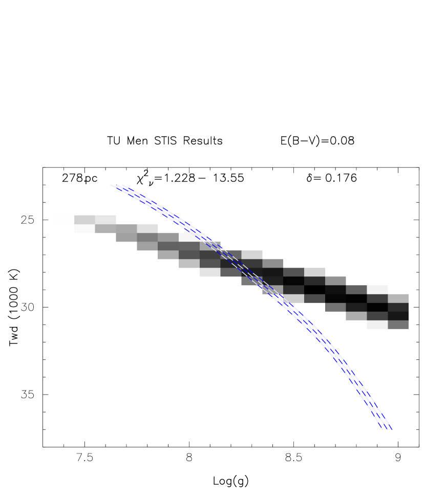
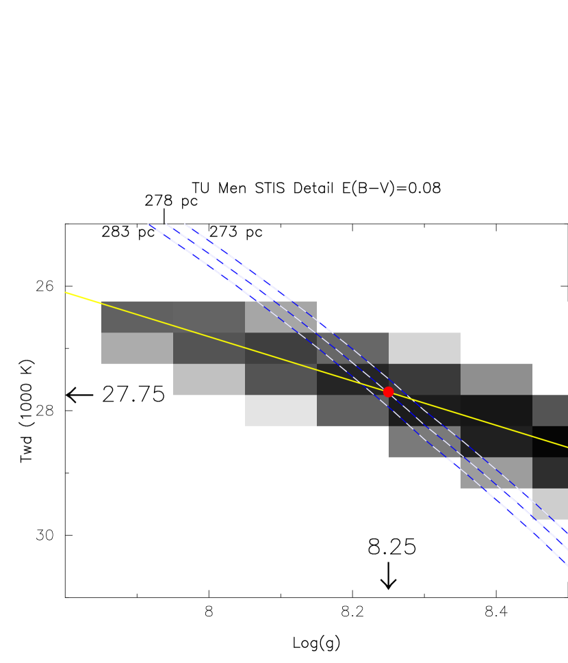
Figure 2: Left. The results of the spectral analysis of the STIS spectrum of TU Men are displayed in the decreasing $T_{\rm wd}$ vs. increasing $Log(g)$ parameter space as a map of the $\chi_{\nu}^{2}$ value. The size of each model is that of a (gray) rectangle of 500 K by 0.1 in Log(g). The least $\chi^{2}$ models are within the gray diagonal area. The other models in white have fast increasing $\chi^{2}_{\nu}$ values towards the lower left and upper right, reaching a maximum value of 13.55. The blue-white dashed triple line indicates a scaling to the Gaia distance of $278\pm 5$ pc: 273 pc (right dashed line), 278 pc (center dashed line), and 283 pc (left dashed line).
Right. A detailed (zoom-in) of the left panel shows the intersection of the least $\chi_{\nu}^{2}$ models with the Gaia distance estimates. The distance has to be between 273 pc (right blue dashed line) and 283 pc (left blue dashed line). The smallest values of $\chi^{2}_{\nu}$ are obtained on the yellow diagonal. The resulting intersection of the 278 pc distance and the least $\chi^{2}_{\nu}$ gives the best fit (represented with a red dot) $Log(g)=8.25$, with $T_{\rm wd}=27,750$ K.

To assess how the uncertainty in the reddening value/extinction law (Sec.3) propagates, we carry out the same analysis with the STIS spectrum of TU Men dereddened assuming now $E(B-V)=0.06$ and $E(B-V)=0.10$. We find, Fig.3, that the uncertainty of $\pm 0.02$ in $E(B-V)$ produces an uncertainty of $\pm 250$ K in $T_{\rm wd}$ and $\pm 0.15$ in $Log(g)$. The rather large uncertainty produced in $Log(g)$ is due to the relative shift between the (dashed) line of the distance and the least $\chi^{2}$ gray diagonal in opposite direction along the $Log(g)$ axis. The moderate uncertainty of $\pm 250$ K is due to their relative shift in the same direction along the $T_{\rm wd}$ axis.

We recall that the errors from the STIS instrument/calibration are only 3% in continuum flux level (see Sec.3), the same order of magnitude as the errors from the Gaia distance. These errors are negligible compared to the uncertainty in flux (18%) propagating from the reddening uncertainty.

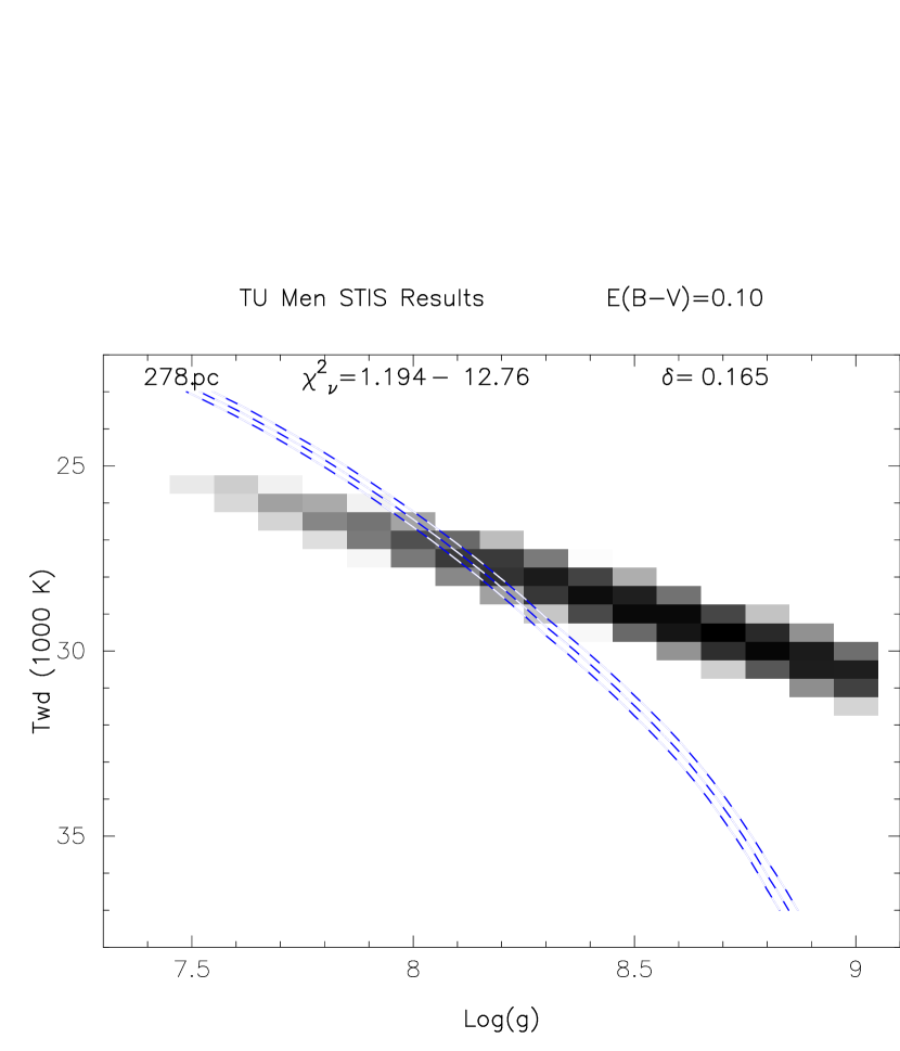
Figure 3: Map of $\chi^{2}_{\nu}$ for the fitting of the STIS spectrum of TU Men assuming $E(B-V)=0.06$ (left panel) and $E(B-V)=0.10$ (right panel). The gray scale, and dashed lines have the same meaning as in Fig.2. The best fit models (gray diagonal) have a slightly lower temperature ($\approx-250$ K) for $E(B-V)=0.06$ and a slightly higher temperature ($\approx+250$ K) for $E(B-V)=0.10$ than for $E(B-V)=0.08$. Due to the scaling of the flux to the distance, the triple dashed line of the Gaia distance also shifts due to the change in the assumed value of $E(B-V)$. As a consequence the best fit is $T_{\rm wd}=28,000$ K and $Log(g)=8.4$ for $E(B-V)=0.06$ (on the left), and $T_{\rm wd}=27,500$ K and $Log(g)=8.1$ for $E(B-V)=0.10$ (on the right). Namely, the uncertainty of $\pm$25% in $E(B-V)$ gives an uncertainty of $\pm 250$ K in $T_{\rm wd}$ and $\pm 0.15$ in $Log(g)$.

We now turn to the statistical errors, from the $\chi^{2}$ minimization technique, for which we consider the problem to be one-dimensional. Namely, while the solution are presented in the two-dimensional parameter space $T_{\rm wd}$ vs $Log(g)$, the constraint $d=278$ pc transforms the problem into a one-dimensional problem: one has to find the least $\chi^{2}$ value along the white-blue dashed line representing the distance. Once one finds the minimum chi square value $\chi^{2}_{\rm MIN}$ along the distance line, the statistical uncertainties on the parameters $T_{\rm wd}$ and $Log(g)$ are obtained by considering all the solutions for which $\chi^{2}_{\rm Min}\leq\chi^{2}\leq\chi^{2}_{\rm Min}+\chi^{2}_{p}(\alpha)$, with $p=1$ and $\alpha=0.01$ (99% confidence) as in Table 3 (see Section 4.2). In Fig.4 we display such a map of $\chi^{2}$ with the statistical uncertainty for the distance line $d=283$ pc (the choice of this distance will become clear in the next paragraph). We obtain a statistical uncertainty of $\pm 350$ K in $T_{\rm wd}$, and $\pm 0.04$ in $Log(g)$. We recapitulate all the errors in Table 4.

The way we assess the cumulative effect of the different uncertainties is illustrated in Fig.4. The red dot represents the lowest temperature and lowest gravity of the solution due to propagation of the cumulative uncertainties of the (i) distance, (ii) reddening and (iii) statistical errors. Similarly, the $\chi^{2}_{\rm Min}+\chi^{2}_{p}(\alpha)$, $d=273$ pc for $E(B-V)=0.06$ gives the highest temperature and highest gravity within the margin of errors. Including the known quantifiable errors in $E(B-V)$, $d$, and $\chi^{2}$, we obtain $T_{\rm wd}=27,750\pm 700$ K, and $Log(g)=8.25\pm 0.20$.

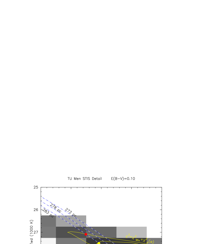
Figure 4: Map of $\chi^{2}$ with statistical errors. In order to assess the statistical errors we consider the least $\chi^{2}_{\rm Min}$ solution for the $d=283$ pc distance, displayed here with the yellow dot. We draw the contour for that value of $\chi^{2}=\chi^{2}_{\rm Min}$. The statistical errors is then obtained by considering the region for which $\chi^{2}_{\rm Min}\leq\chi^{2}\leq\chi^{2}_{\rm Min}+\chi^{2}_{p}(\alpha)$ for $p=1$ and $\alpha=0.01$ (see Table 3). The errors on $T_{\rm wd}$ and $Log(g)$ are then obtained by considering the intersections of the $\chi^{2}_{\rm Min}+\chi^{2}_{p}(\alpha)$ with the $d=283$ pc (dashed) line (the red and blue dots). Overall, the statistical errors have a magnitude of $\pm 350$ K in $T_{\rm wd}$ and $\pm 0.04$ in $Log(g)$.

If we also include the errors introduced from the STIS/instrument and our own modeling we have: $T_{\rm wd}=27,750\pm 1000$ K, and $Log(g)=8.25\pm 0.25$, where we have slightly rounded down the errors. All the errors are listed in Table 4.

Using the mass-radius relation for a $\sim 28,000$K WD (Wood, 1995), we find that $Log(g)=8.25\pm 0.25$ corresponds to a WD mass $M_{\rm wd}\approx 0.77^{+0.16}_{-0.13}M_{\odot}$.

Table 4: Results for $T_{\rm wd}$ and $Log(g)$ with Errors Estimates

	TU Men		SS Aur		SS Aur
	STIS		STIS		FUSE
	$T_{\rm wd}$	$Log(g)$	$T_{\rm wd}$	$Log(g)$	$T_{\rm wd}$	$Log(g)$
Best-fit	27,750	8.25	30,000	8.275	33,375	8.66
	Errors
Source of Errors	$\Delta T_{\rm wd}$	$\Delta Log(g)$	$\Delta T_{\rm wd}$	$\Delta Log(g)$	$\Delta T_{\rm wd}$	$\Delta Log(g)$
distance $d$	$\pm 100$	$\pm 0.02$	$\pm 100$	$\pm 0.02$	$\pm 100$	$\pm 0.02$
$E(B-V)$	$\pm 250$	$\pm 0.15$	$\pm 250$	$\pm 0.15$	$\pm 250$	$\pm 0.15$
instrument	$\pm 100$	$\pm 0.02$	$\pm 100$	$\pm 0.02$	$\pm 500$	$\pm 0.15$
modeling	$\pm 250$	$\pm 0.05$	$\pm 250$	$\pm 0.05$	$\pm 250$	$\pm 0.05$
statistical $\chi^{2}$	$\pm 350$	$\pm 0.04$	$\pm 250$	$\pm 0.025$	$\pm 775$	$\pm 0.06$

Note. — The temperature is in Kelvin and the gravity in cgs.

5.2 SS Aur.

5.2.1 The STIS Spectral Analysis.

For the STIS spectrum of SS Aur, we mask the C ii (1336) and C iv (1550) emission lines, as well as the Si iv (1400) doublet emission feature. We also mask the prominent absorption lines and a portion of the left wing of the Ly$\alpha$ region due to an apparent emission line there. There is no evidence of the C iii (1175) absorption line, we therefore also mask that region. The masked regions are shown in Fig.5 for the best-fit model, for which $Log(g)=8.275$ and $T_{\rm wd}=30,000$ K.

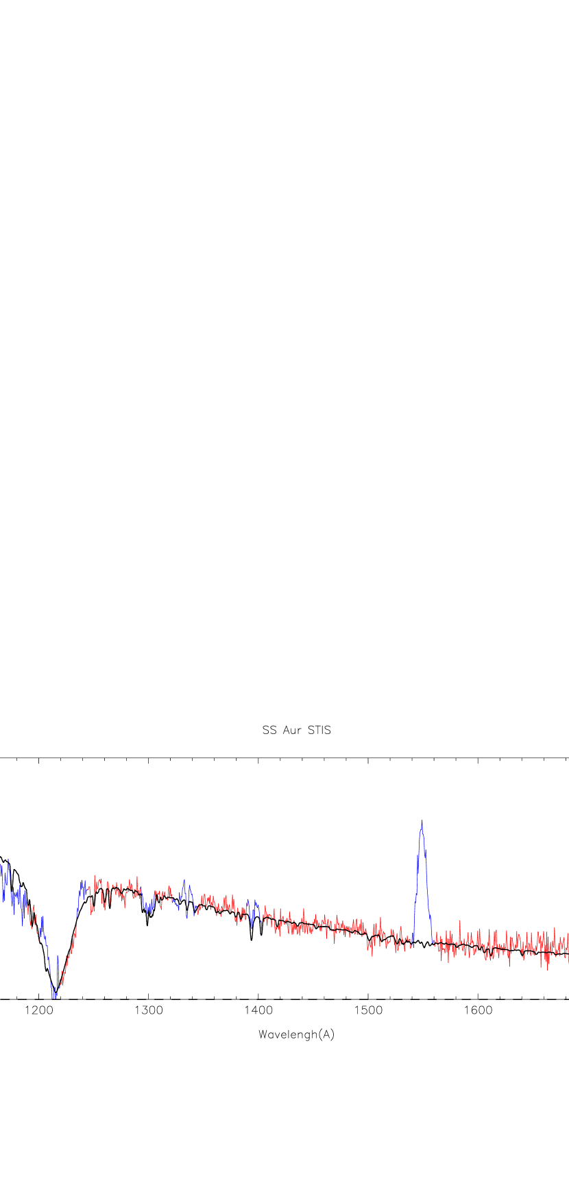
Figure 5: A WD best-fit model (black line) to the STIS spectrum of SS Aur (in red) obtained at quiescence on 2003 Mar 20, 36 days after an outburst. The STIS spectrum exhibits a strong C iv ($\sim$1550) emission line, and possibly some weak N v ($\sim$1240), C ii ($\sim$1336), and Si iv ($\sim 1400$) emission features. Before the WD temperature and gravity fit, we mask emission and absorption lines (in blue). We also mask most of the region below 1200 Å , as the observed flux is significantly smaller than the models and could not be fitted. The model has $T_{\rm wd}=30,000$ K for $Log(g)=8.275$ ($M_{\rm wd}=0.785M_{\odot}$). Fitting the absorption lines is given in section 6, though this model has a projected stellar rotational velocity $V_{\rm rot}sin(i)=400$ km/s, a silicon abundance [Si]=0.2 solar, and a very low carbon abundance (0.001 solar).

We follow the same procedure as for TU Men to assess the best-fit and the errors. The overall results for the STIS spectrum of SS Aur are presented in Fig.6 for $E(B-V)=0.08$, left panel. The statistical errors ($\chi^{2}$, yellow contour lines) yield uncertainties of $\pm 0.025$ in $Log(g)$ and $\pm 250$ K in $T_{\rm wd}$. The uncertainty in the Gaia distance (triple dashed blue line) introduces uncertainties of $\pm 0.02$ in $Log(g)$ and $\pm 100$ K in $T_{\rm wd}$. The systematic uncertainties in the STIS data/instrument are of only $\sim$3%, and introduce errors of the same order of magnitude as for the distance: $\sim\pm 0.02$ in $Log(g)$ and $\sim\pm 100$ K in $T_{\rm wd}$.

The uncertainties of the parameters due to uncertainty in the reddening/extinction law are similar to what we obtain for TU Men: the reddening is the same and the distance (dashed) line intersect the best-fit gray diagonal forming the same angle. For an uncertainty of 0.02 in the reddening $E(B-V)=0.08$, we have uncertainties of $\pm 250$ K in $T_{\rm wd}$ and $\pm 0.15$ in $Log(g)$. All the values are listed in Table 4.

Since the models are built in steps of 500 K in $T_{\rm wd}$ and 0.1 in $Log(g)$, the best-fit model we derive, even if all systematic and statistical errors were zero, can be off by up to 250 K and $0.05$ in $Log(g)$. Namely, there is an intrinsic uncertainty (systematic error) of maximum size $\pm 250$ K in $T_{\rm wd}$ and $\pm 0.05$ in $Log(g)$. Here too, if we linearly add all the uncertainties, overall we have $Log(g)=8.275\pm 0.25$ with $T_{\rm wd}=30,000\pm 1000$ K.

Figure 6: The results of the spectral analysis of the STIS (left panel) and FUSE (right panel) spectra of SS Aur are displayed in the $(log(g),T_{\rm wd})$ parameter space as a map of the $\chi_{\nu}^{2}$ value, as in Fig.2. The yellow contour lines are for the assessment of the statistical errors as in Fig.4. Because the FUSE and STIS spectra have slightly different flux levels and different wavelength coverage, the distance (triple blue dashed lines) does not cross the parameter space in the same manner in both panels. For the STIS spectrum we obtain (left) $Log(g)=8.275$ with $T_{\rm wd}=30,000$ K. For the FUSE spectrum (right) the least-$\chi_{\nu}^{2}$ model with the correct distance yield $Log(g)=8.66$ with $T_{\rm wd}=33,375$ K. The green line in the right panel represents the solution if the continuum flux level in the FUSE spectrum was lowered by 15%, the maximum possible (though unlikely) error due to the FUSE instrument. For a full treatment of the errors in both the FUSE and STIS analyses, see text.

5.2.2 The FUSE Spectral Analysis.

For the FUSE spectrum of SS Aur, we mask all the emission lines from the source (C iii (977), O vi ($\sim$1140)) as well as the sharp airglow/geocoronal emission lines. We mask all the region $\lambda<950$ Å, since the flux in that region also takes negative values (unreliable segments). We also mask all the sharp ISM molecular hydrogen lines. As the C iii (1175) absorption line is absent, we also mask that region.

The results for the $\chi^{2}$ values are presented in Fig.6, also for $E(B-V)=0.08$, right panel. The best-fit model has $Log(g)=8.66$ with a WD temperature $T_{\rm wd}=33,375$ K, it is presented in Fig.7 displaying the masked regions of the spectrum.

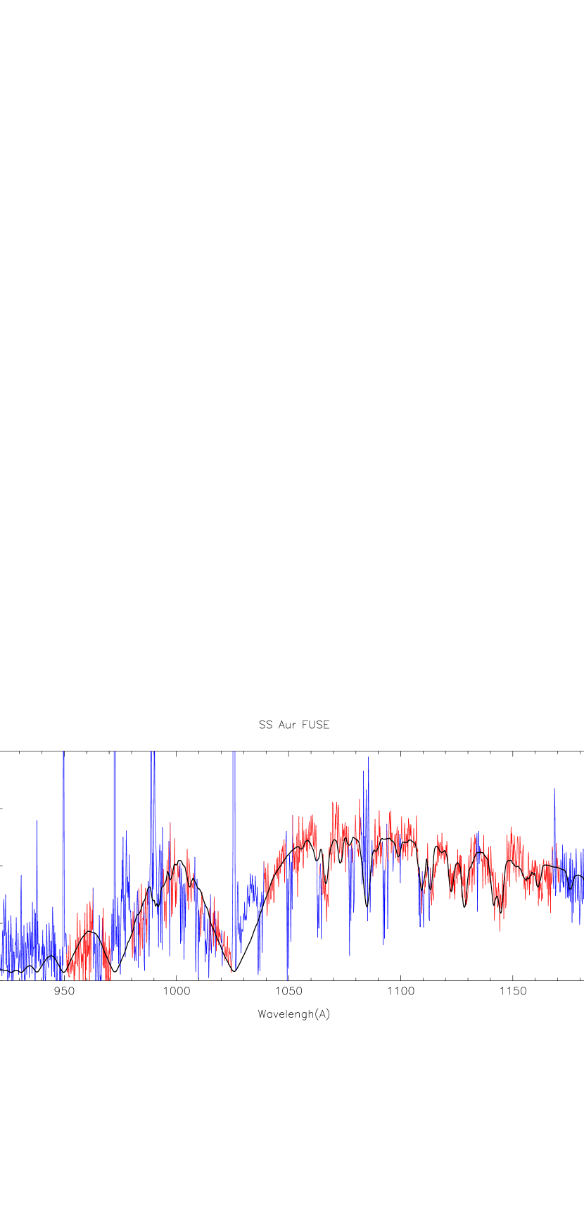
Figure 7: A WD model fit (black line) to the FUSE spectrum of SS Aur (red line) obtained at quiescence on 2002 Feb 13, 28 days after outburst. The spectrum has been dereddened assuming E(B-V)=0.08. Before the spectral fit the sharp ISM absorption lines, the sharp geocoronal emission lines, as well as the broad emission lines from the O vi doublet ($\sim 1032,1038$ Å), and C iii (977 Å), not forming in the photosphere, are all masked and have been colored in blue. Shortward of 950 Å  the flux is unreliable (it even takes some negative values) and has also been masked. The WD fit (Fig.6) yields to $T_{\rm wd}=33,375$ K, for $Log(g)=8.66$ ($M_{\rm wd}=1.045M_{\odot}$). The fitting of the lines is given in section 6, but this model has a projected stellar rotational velocity $V_{\rm rot}sin(i)=400$ km/s with a carbon abundance [C]=0.001$\pm$0.001 solar. All the other species were set to solar abundance.

The uncertainties in the FUSE data can reach up to 15% in the continuum flux level, suffering from a measured flux that is to high by 5-10% in one channel and off by up to 10% in another channel. Whereas one does not expect more than a 5% flux variation between FUSE and STIS spectra (see Sec.3), we assume now that the FUSE flux level is too high by 15% (maximum error) and multiplied the FUSE spectrum by a factor 0.85 before the spectral fit. The result is identical to the one presented in Fig.6 but with the distance increased from 260 pc to 282 pc. Therefore, instead of redrawing a new figure, we draw the $d=282$ pc distance line in green in Fig.6. This lowers the gravity by $\sim$0.15 in $Log(g)$ (from 8.66 to 8.50), and the temperature by $\sim$500 K (from 33,375 K to 32,875 K). In other terms, systematic errors in the FUSE instrument of $\pm 15$% adds an error of $\pm 0.15$ in $Log(g)$ and $\pm 500$ K in $T_{\rm wd}$.

Here too, an uncertainty of 0.02 in the reddening $E(B-V)=0.08$, gives uncertainties of $\pm 250$ K in $T_{\rm wd}$ and $\pm 0.15$ in $Log(g)$. We also assume an intrinsic uncertainty of maximum size $\pm 250$ K in $T_{\rm wd}$ and $\pm 0.05$ in $Log(g)$ due to our models finite size. The statistical errors gives the largest error in $T_{\rm wd}$ of $\pm 775$ K, with $\pm 0.06$ in $Log(g)$. All are listed in Table 4. The sum of the errors is pretty large and yields $Log(g)=8.66\pm 0.43$ with $T_{\rm wd}=33,375\pm 1875$ K. The large error on the temperature is due to the statistical error, which we adopted for a 99% confidence level, and the instrument/calibration errors. We could have adopted a 90% confidence level together with a 5% only of FUSE instrumental errors, which would reduce the total error to $\Delta T\sim 1300$ K, more in line with the STIS spectral analysis. The same is true for the error on $Log(g)$, which would be reduced to $\sim 0.31$. However, we chose the larger errors as we wish to compare the results from the FUSE analysis to that of the STIS analysis (see next subsection).

5.2.3 Comparison.

Since the two (FUSE and STIS) spectra of SS Aur were not obtained at the same epoch after the same outburst, we do not expect the temperature to be the same, but we do expect the gravity to be the same. In order to compare the gravity obtained from the STIS analysis with that obtained from the FUSE analysis, we do not include the errors propagating from the distance and reddening errors, since they must be the same for the STIS and FUSE spectra. Taking into account only the statistical errors, the instrument/calibration errors and the uncertainties from our own modeling (finite steps in $T_{\rm wd}$ and $Log(g)$), one has $T_{\rm wd}=30,000\pm 600$ K with $Log(g)=8.28\pm 0.10$ for STIS, and $T_{\rm wd}=33,375\pm 1525$ K with $Log(g)=8.66\pm 0.26$ for FUSE. The two gravity values do not agree within the error bars. Though the overlap is only missed by a pretty small value, 0.02, it cannot be ignored. This is despite the fact that we chose relatively large values for the FUSE instrument errors and for the statistical error.

A possible explanation for the FUSE higher gravity is the higher temperature itself: if the overall temperature was lower, it would move the gray diagonal in Fig.2 higher up, which would then intersect the distance line at a lower gravity value. We suspect that the possible presence of a hot (second) component contributing to the short wavelengths of FUSE might be responsible for this discrepancy. We do not model such a second component as it would make the FUSE analysis diverge, since the nature and spectral characteristics of this component are completely unknown. In addition, there is no indication of such a component in the STIS spectrum, which may indicate a transient phenomenon. This unknown second emitting component introduces an additional unknown systematic uncertainty which we do not take into account.

6 Abundances and Stellar Rotational Velocity.

6.1 TU Men

We now model the abundance of the elements, starting with TU Men. We first generate a WD model with $Log(g)=8.25$, and $T_{\rm wd}=27,750$ K, and vary the elemental abundances one by one. For each value of an elemental abundance we vary the projected rotational stellar velocity as explained in Sec.4.3. For the STIS spectrum of TU Men, we model the abundances of carbon, nitrogen and silicon. In order to fit the wavelength of (most of) the carbon and silicon lines, the model spectra had to be (red) shifted by +0.6 Å.

As an example of how we derive abundances and broadening velocity by visual examination, we explicitly show the fitting of the Si ii/Si iii ($\sim 1300$ Å) absorption lines in Fig.8. From this figure we obtain [Si]=$0.2\pm 0.1\times$ solar with a velocity broadening of $250\pm 50$ km/s. For this abundance (second row from the top) the depth of the complex silicon spectral feature in the model (red line) is the same as in the observed spectrum (black line). If we consider higher abundances (lower rows) we clearly see how the spectral feature in the model becomes deeper than in the observed spectrum. In that regard, the $\chi^{2}_{\nu}$ technique agrees with the visual examination as shown in the left panel of Fig.9: the least $\chi^{2}_{\nu}$ fit to the silicon $\sim$1300 Å region is minimum for [Si]=0.2$\times$solar. The small flux fluctuations as well as possibly some shallow and sharp absorption lines in the spectrum are of the same amplitude as the flux errors. As a consequence, the best-fit broadening velocity of 250 km/s is found by looking at the 3 individual lines in the silicon feature, as shown with arrows in the right panel of Fig.9. These 3 lines have a depth that is larger than the amplitude of the errors and are braoder than the spectral binning of $0.58$Å. While the visual examination clearly shows that the best-fit is for [Si]$\approx 0.1-0.2$ for $V=250$ km/s, the $\chi^{2}$ becomes smaller for the higher velocity models, $V\sim 350$ km/s and higher, see left panel of Fig.9. The reason the $\chi^{2}_{\nu}$ minimization technique gives a much higher velocity is that it cannot identify actual lines and differentiate them from the small fluctuations. As the velocity broadening increases, the $\chi^{2}_{\nu}$ decreases sharply until it reaches about 300 km/s, at higher velocities the $\chi^{2}_{\nu}$ decreases only by a few percent at most, which is not significant enough to assess which of these models, say e.g. V=300 km/s vs. V=600 km/s, is the best. The important point, however, is that, irrelevant to the broadening velocity (250 km/s vs. 450 km/s), a best fit of [Si]=0.2 is obtained for both the $\chi^{2}_{\nu}$ technique and the visual examination. It becomes clear that for a higher abundance and higher velocity, e.g. [Si]=0.5 with V=350 km/s - the lower right panel in Fig.8, there is a fairly gross discrepancy between the model (red line) and data (black line): a higher velocity with a higher abundance degrades the fit.

Figure 8: Example of fitting absorption lines by visual examination: the fitting of the Si ii & Si iii ($\sim$ 1300 Å) absorption feature in the STIS spectrum of TU Men is shown explicitly. The STIS spectrum is in black, the WD model is in red with a temperature of 27,750 K and an effective surface gravity of $Log(g)=8.25$. Each of the 25 panels displays the same wavelength coverage: from 1280 Å to 1320 Å. The silicon abundance increases from 0.1 solar (top row) to 0.5 solar (bottom row) in steps of 0.1; the velocity broadening of the lines is increased from 150 km/s (far left) to 350 km/s (far right) in steps of 50 km/s. A visual inspection of the panels immediately shows that the 150 km/s and 350 km/s broadening velocities can be excluded. Similarly it is clear that the abundances [Si]=0.4 and 0.5 solar yield to deeper absorption features (which is more apparent when looking at the 350 km/s broadening). The best-fit is for [Si]$\approx 0.1-0.2$ solar with $V=250$ km/s. Due to the finite size of our grid of models we adopt the solution [Si]= $0.2\pm 0.1$ solar with $V=250\pm 50$ km/s. Note that the $V=50$, 100, 400, 450, and 500 km/s, as well as the abundances [Si]=0.6, 0.7, 0.8, 0.9, and 1.0 are not shown for clarity.

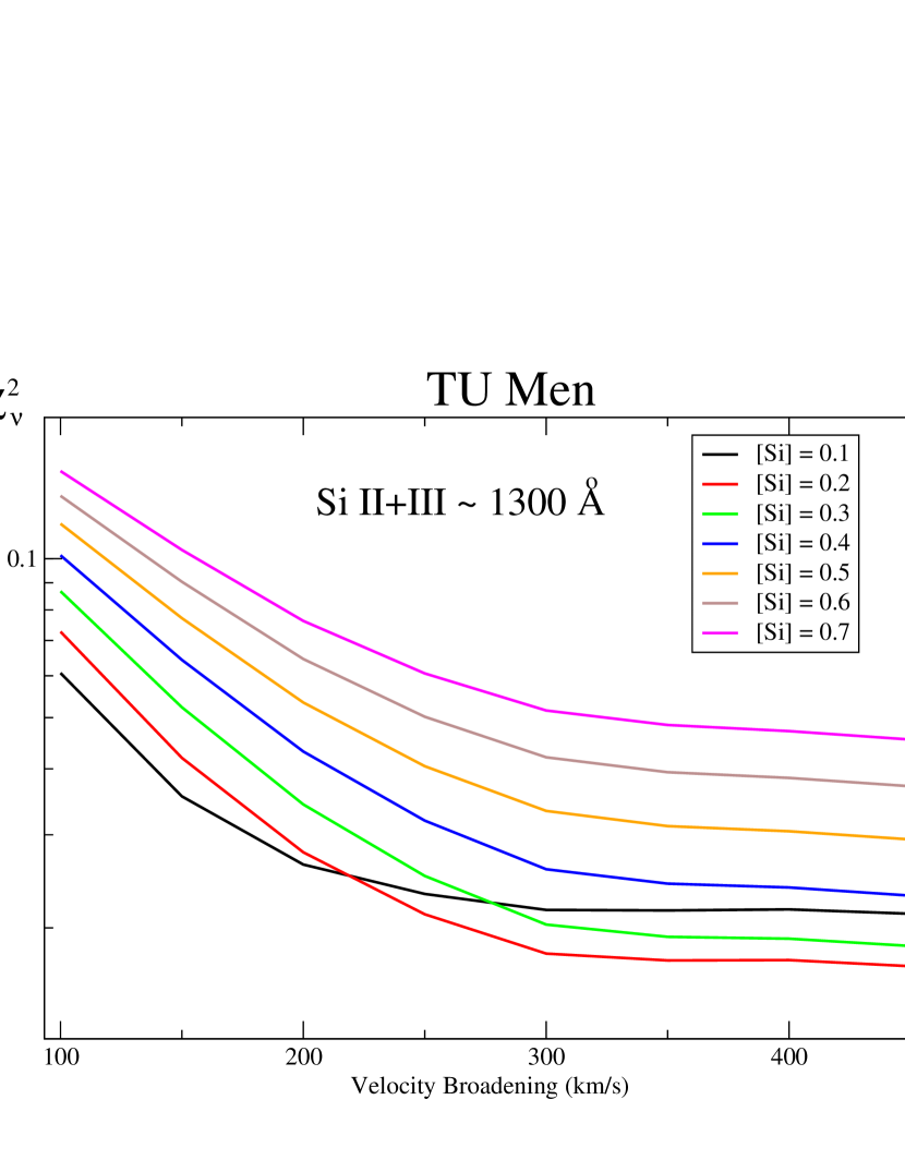
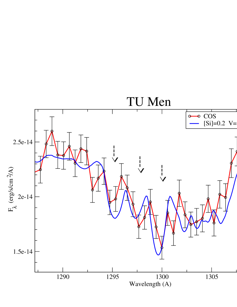
Figure 9: Fitting the Si ii + Si iii absorption lines at $\sim 1300$ Å (as shown in Fig.8) yields to a low $\chi^{2}_{\nu}$ best-fit for the largest values of the broadening velocity, as shown on the left. This is due to the spectral binning (0.58 Å) and errors having the same width and amplitude as the small flux fluctuation of the spectrum, as shown on the right, without being able to differentiate between fluctuations and actual absorption lines. The visual examination (done in Fig.8) is carried out by ensuring that actual absorption lines, as the ones indicated by the three arrows in the right panel, are matched in the fitting (within the given accuracy of the flux errors and spectral binning size). In spite of that the $\chi^{2}_{\nu}$ minimization technique does agree with the visual examination that the silicon abundance is small: [Si]=0.2. At higher broadening velocity the [Si]=0.2 model does not reproduce these features in Fig.8. A higher velocity with a higher abundance also does not provide a fit visually good enough (as can also be seen in the previous figure).

We also illustrate, in Fig.10, how we fit the carbon abundance based mainly on the C ii ($\sim 1325$ & $\sim 1336$) absorption lines. The C ii ($1325$) absorption line agrees best with [C]=$0.1$ (solar) and $V=150$ km/s, and somewhat also with [C]=$0.2$ and $V=200$ km/s. As to the C ii ($1336$) line, its bottom agrees well with [C]=$0.2$ and $V=200$ km/s, and somewhat also with [C]=$0.3$ and $V=250$ km/s. The shallower part, however, can be fitted with [C]=$0.5-0.6$ with $V=450-500$ km/s. The two different widths may indicate a second component polluting the line, such as e.g. ISM absorption. Indeed, the local ISM (within 100 pc) could contribute to the C ii (1336) line (as well as to the Si ii (1260) line) (Redfield & Linsky, 2004), and the shape of the C ii (1336) line indicates a possible (less deep) second component. Therefore, for carbon, we have [C]=$0.2\pm 0.1$ with $V=200\pm 50$ km/s. In a similar manner we fit the nitrogen lines N i ($\sim 1165-1170$).

Figure 10: The fitting of the C ii ($\sim$1325 & $\sim$1336) absorption lines in the STIS spectrum of TU Men is shown as a function of the carbon abundance [C] and velocity broadening $V$. The C ii (1325) line is best fitted with [C]=0.1 and $V=150$ km/s (left panel). The C ii (1336) doublet agrees better with [C]=0.2 and $V=200$ km/s (middle panel), when one fits the lower narrower part of the absorption feature. The broader (and shallower) part of the feature agrees with [C]=0.5-0.6 and $V=450-500$ km/s (right panel). Such a large velocity broadening is in disagreement with all the other absorption lines, raising the possibility that the broadening is due to a second component.

The best fit to the absorption lines gives: [C]=$0.2\pm 0.1$ solar, [Si]=$0.2\pm 0.1$ solar, and [N]=$20\pm 10$ solar, with an overall matching broadening velocity of $\sim 225\pm 75$ km/s. The final result of this model (temperature, gravity, abundances and velocity broadening) was presented in Fig.1. While fitting of the absorption lines is further presented in the 2 panels of Fig.11, for wavelengths below 1280 Å (since the remaining lines are already presented in Figs.8 & 10). For comparison, in Fig.11, we also show a solar abundance model. The C iii $\lambda\sim$1175 line seems to possibly have a blue shifted emission peak in its center (first panel). While we fit most of the silicon lines, the Si ii (1260) line is deeper than in our model. From the shape of the line (showing a sharp bottom) and from the above mention ISM absorption, it is likely that this line is also affected by ISM absorption.

Figure 11: The fits to carbon, silicon, and nitrogen absorption lines are shown in details. The HST spectrum is in black, the model is shown in red, and for comparison a solar abundance model is shown with the blue dashed line. The left panel shows the blue wing of the Lyman $\alpha$ region and the fitting of (mainly) the nitrogen lines; the right panel shows the fitting of silicon lines. The abundances are as indicated in the upper right in each panel. The C iii (1175) may have emission at the bottom of its absorption line.

We also check how the error on the temperature and gravity affect the error on the abundances (propagation of errors). We compare the absorption lines of carbon [C]=0.2, silicon [Si]=0.2, and nitrogen [N]=20 for the two limiting cases (within the error bars, see Table 5): $T_{\rm wd}=26,750$ K with $Log(g)=8.00$, against $T_{\rm wd}=28,750$ K with $Log(g)=8.50$. We find that the difference in the absorption lines profiles between these two models is significantly smaller than the size of the abundance steps in the models. The propagation of the errors in $T_{\rm wd}$ and $Log(g)$ is negligible compared to the errors we adopted for the abundances.

6.2 SS Aur

To fit the abundances in the STIS spectrum of SS Aur, we set $T_{\rm wd}=31,000$ K with $Log(g)=8.50$, this corresponds to the upper values of the STIS results within the errors (see Table 5). For SS Aur, we fit the abundances of silicon and carbon, following the same procedure described for TU Men, namely, we vary the abundance of Si and C one by one, and for each abundance value, we vary broadening velocity (as already explained and illustrated in Fig.8).

The fitting of the lines in the STIS spectrum of SS Aur is illustrated in Fig.12. We display a solar abundance model (green), and a low silicon abundance model with different broadening velocity $V=200$ km/s (blue), $V=300$ km/s (red), and $V=400$ km/s (orange). We note (left panel) that the Si i ($\sim$1265) line agrees with $V=200$ km/s, while the Si ii+Si iii complex absorption feature ($\sim 1300$) agrees with $V=300$ & 400 km/s. As for TU Men, the Si i (1260) is possibly from the ISM. The C i & Si ii lines ($\sim 1250$) are possibly affected by some emission (N v $\sim$1240), as the continuum there doesn’t match, but while the carbon could be solar, the silicon line is definitely much sharper (ISM?). Both the C ii ($\sim$1335) and Si iv ($\sim$1400) lines also reveal broad emission (right panel), but in both cases the absorption feature seems less deep than solar. In addition the C ii ($\sim$1325), C i ($\sim$1330), and Si iii ($\sim$1343 & $\sim$1365) all agree well with and a low silicon and carbon abundances. Overall, the fitting of the absorption lines is consistent with a very low carbon abundances($\sim 0.001$ solar), and agrees with a silicon abundances [Si]=$0.1^{+0.1}_{-0.05}$. We assess a broadening velocity $V\sim 300\pm 100$ km/s.

We compare this abundance model with a similar one in which we set $T_{\rm wd}=29,000$ K with $Log(g)=8.00$. These values of $T_{\rm wd}$ and $Log(g)$ correspond to the lower end of the STIS results for SS Aur within the errors. As for the TU Men, we find that the difference between the lines profiles of the two models (31,000 K and 29,000 K) is well within the error bars of the abundances (i.e. the size of the step by which we increase the abundances). Namely, we obtain that the errors on the abundances propagating from the errors on $T_{\rm wd}$ and $Log(g)$ are negligible as they are smaller than the size of the abundances step.

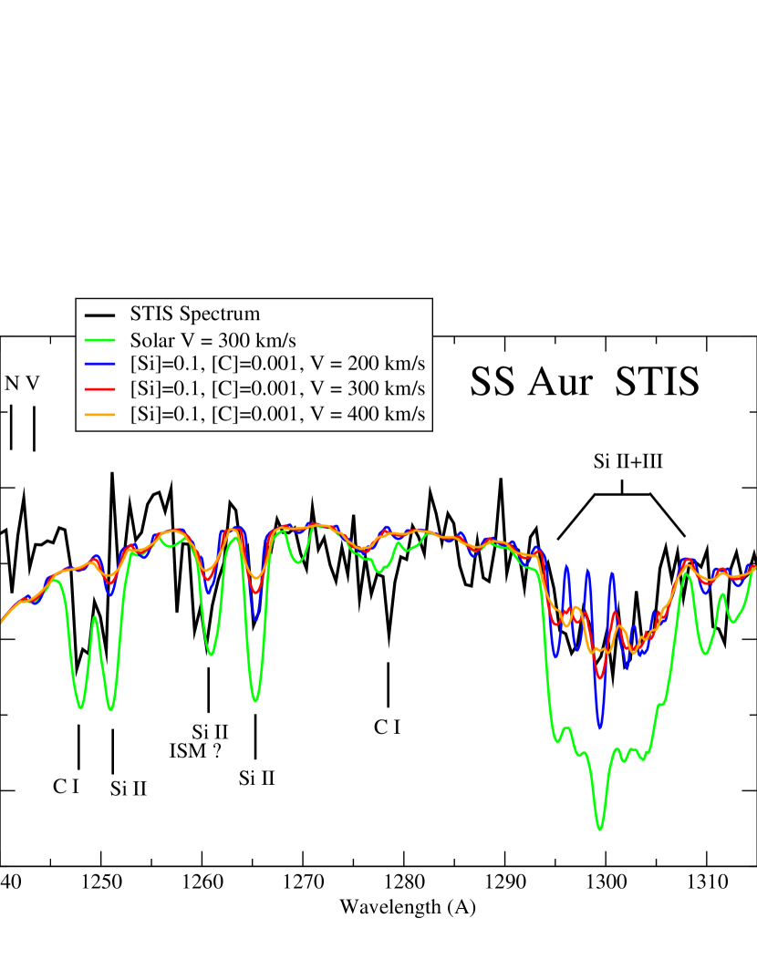
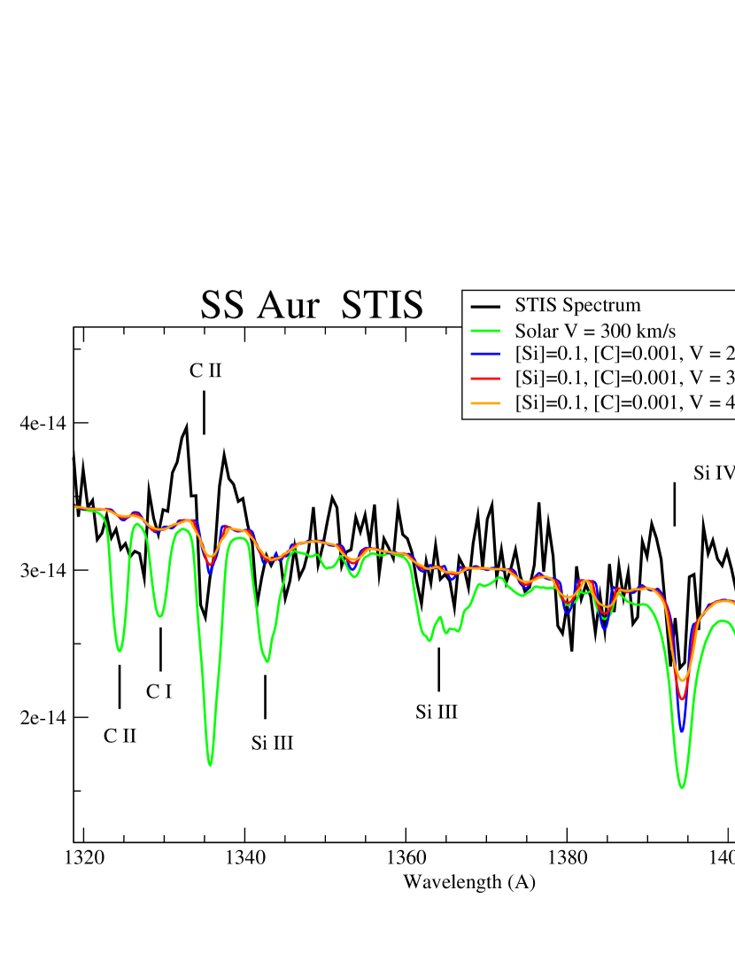
Figure 12: Detailed regions of the spectral fit are displayed, showing different model fits to the STIS spectrum (in black). The model has $T_{\rm wd}=31,000$ K with $Log(g)=8.5$, the abundances and broadening velocities are as indicated (color-coded). The fit to the absorption lines is discussed in the text.

For the abundance analysis of the FUSE spectrum of SS Aur, we set $T_{\rm wd}=32,500$ K, with $Log(g)=8.5$, the same $Log(g)$ assumed for the STIS spectrum of SS Aur. The fitting of the abundances yields to solar abundances, except for carbon, which gives [C]=$0.001\pm 0.001$. This is based mainly on the C iii (1175) absorption line, but a detailed look at absorption lines (see Fig.13) shows that another carbon absorption line ($\sim$1140 Å) is also better fitted with a very low carbon abundance. On the other hand, a carbon absorption feature near 1165 Å seems to be better fitted with solar carbon abundance. That region, however, is also affected by ISM absorption lines. For the projected stellar velocity we obtained $\sim 500\pm 100$ km/s based on the (unaffected by ISM) silicon absorption lines (Fig.14).

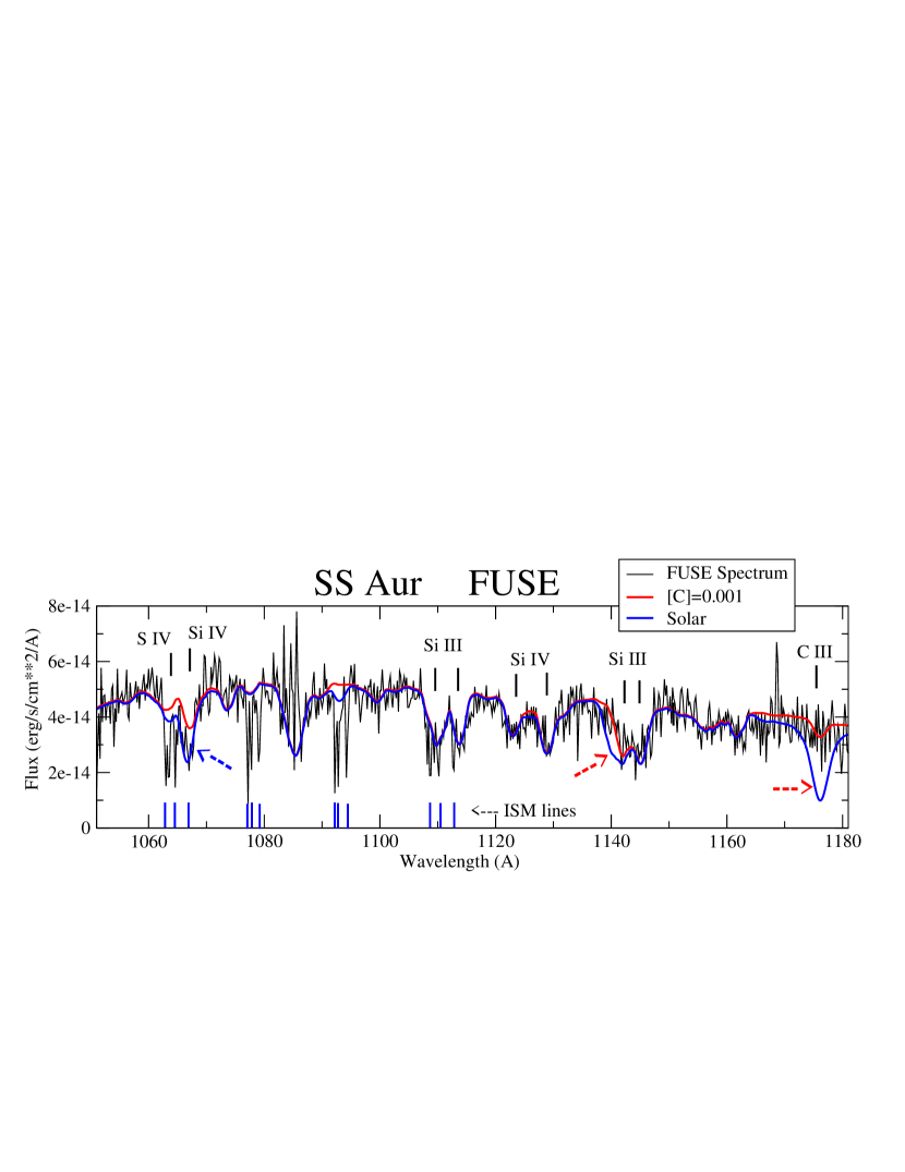
Figure 13: A detailed portion of the FUSE (in black) spectral fit is displayed showing a solar abundance model (in blue) compared to a low carbon abundane model (in red). In order to fit the C iii (1175 Å) line (red arrows on the right), the carbon abundance was lowered to 0.001 (in solar units), while the remaining species were left at their solar value. The low carbon also improves the fit to the C i absorption feature near 1139 Å (red arrow), but degrades the fit to the C ii feature near 1163-66 Å (blue arrow on the left). That C ii feature is also affected by ISM absorption. The model has $T_{\rm wd}=32,500$ K with $Log(g)=8.5$ with a rotational velocity of 400 km/s.

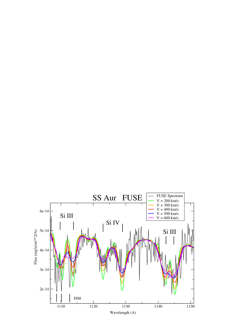
Figure 14: The region of the silicon absorption lines unaffected by ISM absorption (1120 Å - 1150 Å) is shown for different broadening velocities, solar silicon abundance and low (0.001) carbon abundance. The fitting gives a velocity of $500\pm 100$ km/s. The ISM lines are marked at the bottom left of the panel. The model has $T_{\rm wd}=32,500$ K with $Log(g)=8.5$.

Next, we compute a model with $T_{\rm wd}=35,250$ K and $Log(g)=9.1$, i.e. the upper limit of the FUSE solution (within its error bars) and a model with $T_{\rm wd}=31,500$ K and $Log(g)=8.2$, i.e. the lower limit of the FUSE solution (also within its error bars, see Table 5). We set up solar abundances, except for [C]=0.001 solar. The hotter model exhibits slightly shallower Si iii ($\sim$1145) lines and slightly deeper Si iii ($\sim$1110) lines than the colder model, but here too the difference is negligible when compared to the step size of the the abundance. Namely, the propagation of the errors in temperature and gravity on the silicon and carbon abundance is negligible.

7 Discussion and Conclusion

We summarize the results in Table 5, where we also include the mass and radius of the WD as derived from the $Log(g)$ values using the mass-radius relation for non-zero WD (Wood, 1995). For SS Aur the FUSE analysis yielded a higher temperature and, therefore, a higher gravity than the STIS analysis. The difference in gravity was not within the limits of our error analysis. A possible cause for the higher temperature, could be a second (hot) component contributing only to the shortest wavelength of the FUSE spectrum.

Table 5: FUV Spectral Analysis Results

Parameter	Units	TU Men	SS Aur	SS Aur
		STIS	STIS	FUSE
$T_{\rm wd}$	(K)	$27,750\pm 1000$	$30,000\pm 1000$	$33,375\pm 1875$
$Log(g)$	(cgs)	$8.25\pm 0.25$	$8.275\pm 0.25$	$8.66\pm 0.43$
$\chi^{2}_{\nu}$		1.247	1.324	0.959
$M_{\rm wd}$	$(M_{\odot})$	$0.77^{+0.16}_{-0.13}$	$0.785_{-0.13}^{+0.17}$	$1.045_{-0.28}^{+0.21}$
$R_{\rm wd}$	(km)	$7550^{+1610}_{-1270}$	$7430^{+1620}_{-1290}$	$5490^{+2205}_{-1835}$
$[$C$]$	Solar	$0.2\pm 0.1$	$<<1$	$<<1$
$[$N$]$	Solar	$20\pm 10$	—	—
$[$Si$]$	Solar	$0.2\pm 0.1$	$0.1_{-0.05}^{+0.1}$	1
$V_{\rm rot}sin(i)$	(km/s)	$225\pm 75$	$300\pm 100$	$500\pm 100$

Note. — The STIS and FUSE spectra of SS Aur were not obtained during the same epoch, as a consequence the abundances and temperature of the WD in column 4 & 5 are not expected to agree. The masses and radii were obtained from the values of $Log(g)$ using the mass-radius relation for non-zero temperature WD (Wood, 1995). Since for each spectrum the solution is a narrow diagonal band in the $T_{\rm wd}$ vs $Log(g)$ parameter space, the larger temperature (+) is associated with the larger gravity (+), larger WD mass (+), and smaller WD radius (-), and vice versa.

The dereddened STIS snapshots of SS Aur and TU Men were analyzed in Sion et al. (2008), who considered WD models, disk models as well as WD+disk models, but the disk only degraded the solution, confirming that the observed spectrum is that of an exposed WD. Only solar composition WD models were fitted to the STIS spectra assuming $Log(g)=8.0$ and $8.3$ for TU Men, and $Log(g)=8.7$ and $8.8$ for SS Aur. In Godon et al. (2008) we analyzed the combined FUSE+STIS spectrum of SS Aur, considering values of $Log(g)=8.3$ to $8.9$ yielding a temperature $T_{\rm wd}=27,000$ K to 34,000 K for a distance of 200-250 pc. In that work, we did not considered non-solar abundances for SS Aur. These previous results (Godon et al., 2008; Sion et al., 2008) for the temperature and gravity of SS Aur and TU Men are in line with our present global analysis, however, they only represent a small number of data points when compared to Figs.2 & 6. Overall, the present work comes to improve and enlarge our FUV spectral analysis of TU Men and SS Aur.

We reconsider here our interpretation that the WD in SS Aur has solar abundances, and show in the present work that data implies subsolar silicon abundance as well as possibly subsolar carbon abundance. Our most important result is that both TU Men and SS Aur display subsolar C and Si abundances, in addition TU Men also presents evidence of suprasolar nitrogen abundance, i.e. evidence of CNO processing. We do not find evidence of elevated nitrogen abundances for SS Aur. On the contrary, we find that the red wing of the N ii $\lambda$ 1085 absorption feature (Fig.13) agrees well with solar abundances, though the rest of the feature is possibly contaminated with some geocoronal component.

The STIS snapshots of SS Aur and TU Men have, respectively, an exposure time of 600 s and 900 s. As a consequence the absorption lines are not broadened by the WD orbital motion. But the STIS snapshots have a low resolution which might affect some weak and sharp absorption lines, but cannot be responsible for the absence of C ii (1175) in SS Aur or the shallow Si ii+iii (1300) absorption feature (unlike COS, STIS also does not suffer from much geocoronal emission O i at 1300 Å).

We found that both the FUSE and STIS spectra of SS Aur agree with a velocity broadening of 400 km/s within the limits of error bars, with the lines in the FUSE spectrum being (on average) 200 km/s broader than in the STIS spectrum. The FUSE spectrum of SS Aur was obtained over a (raw) period of about 8 hr, or almost two complete binary orbits. The reason for the different broadening velocities in the FUSE and STIS spectra is likely due to the combined effect of the WD orbital velocity ($K_{1}=70\pm 10$ km/s, see Table 1) and the different instrumental broadening. We considered looking at the individual exposures (orbits) of the FUSE spectrum of SS Aur, but their poor S/N (when not co-added) prevented us from being able to properly fit the absorption lines.

For TU Men, $K_{1}$ could be twice as large, but since the STIS snapshot lasted only 900 s, broadening due to the WD motion need not to be taken into account. Regardless of that, the STIS snapshots have a resolution of $R\sim 1000$, with a binning of 0.58 Å. At the STIS wavelengths, a $\Delta\lambda$ of 0.58 Å corresponds to a velocity of $\sim$100-150 km/s. For both objects, we can therefore take this velocity ($\sim 150$ km/s) as being the lower resolution limit for the measurement of line broadening or measurement of the projected stellar rotational velocity.

The high N/C abundance ratio implies CNO processing which elevates the abundance of nitrogen and depletes the abundance of carbon. Interstingly, while the dwarf novae TU Men and VW Hyi reveal prominent C iv emission line profiles in their FUV spectra during quiescence, their accreting white dwarfs show large N/C photospheric abundance ratios and subsolar C (Sion et al., 1997; Long & Gilliland, 1999). The dwarf nova U Gem, which lies above the CV period gap, reveals no such C iv emission line in either outburst or quiescence (Panek & Holm, 1984). Yet, the donor star in U Gem is carbon deficient while the donor star in VW Hyi appears to have solar carbon abundance (Harrison, 2016). The carbon deficiency in the photosphere of the white dwarf in VW Hydri could be, at least in part, an effect of gravitational diffusion (diffusion time scales of metals at the bottom of the convection zone in WDs can be as short as $\sim days$, see e.g. Heinonen et al., 2020, for a short review and recent developments). In our synthetic spectral modeling we do not include emission line modeling capability but it is virtually certain that this C iv emission does not form on the accreting white dwarf itself. Instead, it may form in the inner disk or an accretion disk corona during quiescence when the accretion disk is optically thin. It cannot be entirely ruled out that the C iv emission forms in the boundary layer between the inner disk and white dwarf. But even if the C abundance implied by the C iv emission line strength is solar, the presence of suprasolar N still points toward CNO processing.

The exact origin of nonsolar abundances is not known, but several hypothesis have been suggested (see e.g. Gänsicke et al., 2003, for a short review). For example the possibility of anomalous abundances in the accreting material itself, either from a (recent) nova outburst (where the donor star is contaminated by the material ejected from the nova explosion of the WD), or related to the nuclear evolution of the secondary (if the donor was originally more massive than the WD, resulting in a transitional phase of unstable thermal timescale mass transfer, it is then stripped from its outer layer). The secondary star in VW Hydri has a solar carbon abundance (Harrison, 2016), yet the accreting white dwarf in VW Hydri has a large N/C abundance ratio as expected for hot CNO burning. While we do not know the carbon abundance of the donor secondary in TU Men, the accreting white dwarf photosphere also has a suprasolar N/C abundance ratio. This result quite possibly could be pointing toward the origin of the elevated N and depleted C in the white dwarf itself (Sion & Sparks, 2014). This may support a scenario whereby the elevated N/C ratio does not arise from the peeling away by mass transfer of the CNO processed core of an originally more massive donor secondary but instead in the WD itself from the hot CNO processing of many previous nova explosions (Sion et al., 1998; Sion & Sparks, 2014). It is important to remark also that, while other CVs have exhibited an anomalously high N/C ratio, TU Men is the only dwarf nova with an exposed WD in the CV period gap.

As to SS Aur, the lack of strong carbon absorption lines in the FUSE and STIS spectra strongly contrasts with the presence of normal looking CO absorption in the K-band from its secondary (Howell et al., 2010), and C iv emission line (see Fig.5) from disk, disk corona or boundary layer.

Despite not having phase-resolved high S/N spectra (available only for a few of systems, such as VW Hyi and U Gem), we have presented further evidence of subsolar C abundances in two accreting white dwarfs, in the dwarf novae TU Men and SS Aur. As part of our HST Archival Program research (see Acknowledgements below), we are currently carrying out chemical abundance studies in more systems with exposed accreting white dwarfs in order to further understand the physics of white dwarf accretion and the evolution of cataclysmic variables.

References

- Allard et al. (2020) Allard, N.F., Kielkopf, J.F., Xu, S. et al. 2020, MNRAS, 494, 868
- Avni (1976) Avni, Y. 1976, ApJ, 210, 642
- Bateson et al. (2000) Bateson, F., McIntosh, R., Stubbings, R. 2000, PVSS, 24, 48
- Bohlin et al. (2014) Bohlin, R.C., Gordon, K.D., Tremblay, P.-E. 2014, PASP, 126, 711
- Bruch & Engel (1994) Bruch, A., & Engle, A. 1994, A&AS, 104, 79
- van Dixon et al. (2007) van Dixon, W. Sahnow, D.J., Barrett, P.E., et al. 2007, PASP, 119, 527
- Fitzpatrick (1999) Fitzpatrick, E.L. 1999, PASP, 111, 63
- Fitzpatrick & Massa (2007) Fitzpatrick, E.L., & Massa, D. 2007, ApJ, 663, 320
- Gänsicke et al. (2003) Gänsicke, B.T., Szkody, P., de Martino, D. et al. 2003, ApJ, 594, 443
- Gänsicke et al. (2005) Gänsicke, B.T., Szkody, P., Howell, S.B. & Sion, E.M. 2005, ApJ, 629, 451
- Gänsicke et al. (2018) Gänsicke, B.T., Koester, D., Farihi, J., Toloza, O. 2018, MNRAS, 481, 4323
- Godon et al. (2017a) Godon, P., Shara, M.M., Sion, E.M., & Zurek, D. 2017a, ApJ, 850, 146
- Godon et al. (2017b) Godon, P., Sion, E.M., Balman, S., Blair, W.P. 2017b, ApJ, 846, 52
- Godon et al. (2008) Godon, P., Sion, E.M., Barrett, P.E. et al. 2008, ApJ, 679, 1447
- Godon et al. (2012) Godon, P., Sion, E.M., Levay, K. et al. 2012, ApJS, 203, 29
- Harrison (2016) Harrison, T.E. 2016, ApJ, 833, 14
- Harrison et al. (2000) Harrison, T.E., McNamara, B.J., Szkody, P., & Gilliland, R.L. 2000, AJ, 120, 2649
- Heinonen et al. (2020) Heinonen, R.A., Saumon, D., Daligault, J., Starrett, C.E., Baalrud, S.D., & Fontaine, G. 2020, ApJ, 896, 2
- Howell et al. (2010) Howell, S.B., Harrison, T.E., Szkody, P., & Silvestri, N.M. 2010, AJ, 139, 1771
- Hubeny (1988) Hubeny, I. 1988, CoPhC, 52, 103
- Hubeny & Lanz (1995) Hubeny, I., & Lanz, T. 1995, ApJ, 439, 875
- Hubeny & Lanz (2017a) Hubeny, I., & Lanz, T. 2017a, A Brief Introductory Guide to TLUSTY and SYNSPEC, arXiv:1706.01859
- Hubeny & Lanz (2017b) Hubeny, I., & Lanz, T. 2017b, TLUSTY User’s Guide II: Reference Manual, arXiv:1706.01935
- Hubeny & Lanz (2017c) Hubeny, I., & Lanz, T. 2017c, TLUSTY User’s Guide III: Operational Manual, arXiv:1706.01937
- Kraft & Luyten (1965) Kraft, R.P., & Luyten, W.J. 1965, ApJ, 142, 1041
- Lake & Sion (2001) Lake, J., & Sion, E.M. 2001, AJ, 122, 1632
- Lampton et al. (1976) Lampton, M., Margon, B., Bowyer, S. 1976, ApJ, 208, 177
- Lindergren et al. (2018) Lindergren, L, Hernández, J., Bombrun, A. et al. 2018, A&A, 616, 2
- Long & Gilliland (1999) Long, K.S., & Gilliland, R.L. 1999, ApJ, 511, 916
- Long et al. (2006) Long, K.S., Brammer, G., & Fronning, C.S. 2006, ApJ, 648, 558
- Long et al. (2009) Long, K.S. et al. 2009, ApJ, 697, 1512
- Luri et al. (2018) Luri, X., Brown, A.G.A., Sarro, L.M. et al. 2018, A&A, 616, 9
- Mennickent (1995) Mennickent, R.E. 1995, A&A, 294, 126
- Moos et al. (2000) Moos, H.W., Cash, W.C., Cowie, L.L. et al. 2000, ApJ, 538, L1
- Pala et al. (2017) Pala, A.F., et al. 2017, MNRAS, 466, 2855
- Panek & Holm (1984) Panek, R.J. & Holm, A.V. 1984, ApJ, 277, 700
- Ramsay et al. (2017) Ramsay, G., Schreiber, M.R., Gänsicke, B.T. et al. 2017, A&A, 604, 107
- Redfield & Linsky (2004) Redfield, S., & Linsky, J.L. 2004, ApJ, 602, 776
- Ritter & Kolb (2003) Ritter, H., Kolb, U. 2003, A&A, 404, 301 (update RKcat7.24, 2016)
- Sahnow et al. (2000) Sahnow, D.J., Moos, H.W., Ake, T.B., et al. 2000, ApJ, 538, L7
- Sasseen et al. (2002) Sasseen, T.P., Hurwitz, M., Dixon, W.V., Airieau, S. 2002, ApJ, 566, 267
- Savage & Mathis (1979) Savage, B.D., & Mathis, J.S. 1979, ARA&A, 17, 73
- Selvelli & Gilmozzi (2013) Sevelli, P., & Gilmozzi, R. 2013, A&A, 560, 49
- Sembach (2001) Sembach, K.R., et al. 2001, ApJ, 561, 573
- Shafter (1983) Shafter, A.W. 1983, PhD Thesis, UCLA.
- Shafter & Harkness (1986) Shafter, A.W., & Harkness, R.P. 1986, AJ, 92, 658
- Sion et al. (1997) Sion, E.M. et al. 1997, ApJ, 480, L17
- Sion et al. (1998) Sion, E.M. et al. 1998, ApJ, 496, 449
- Sion et al. (2004) Sion, E.M. et al. 2004, AJ, 128, 1834
- Sion et al. (2008) Sion, E.M., Gänsicke, B.T., Long, K.S. et al. 2008, ApJ, 681, 543
- Sion & Sparks (2014) Sion, E.M. & Sparks, W.M. 2014, ApJ, 796, L10
- Smak (2006) Smak, J.I. 2006, Acta Astronomica, 56, 277
- Stolz & Schoembs (1984) Stolz, B., & Schoembs, R. 1984, A&A, 132, 187
- Tappert et al. (2003) Tappert, C., Mennickent, R.E., Arenas, J. et al. 2003, A&A, 408, 661
- Tody (1993) Tody, D. 1993, in ASP Conf. Ser. 52, Astronomical Data Analysis Software and Systems II, ed. R.J. Hanisch, R.J.B. Brissenden, & J. Barnes (San Fransisco, CA;ASP), 173
- Verbunt (1987) Verbunt, F. 1987, A&AS, 71, 339
- Wood (1995) Wood, M.A. 1995, in Proc. 9th Europ. Workshop on WDs, 443, White Dwarfs, ed. D. Koester & K. Werner (Berlin: Springer), 41