The $\big{\langle}A^{2}\big{\rangle}$ Asymmetry and Gluon Propagators
in Lattice $SU(3)$ Gluodynamics at $T\simeq T_{c}$.

Abstract

We study numerically the chromoelectric-chromomagnetic asymmetry of the dimension two $A^{2}$ gluon condensate as well as the infrared behavior of the gluon propagators at $T\simeq T_{c}$ in the Landau-gauge $SU(3)$ lattice gauge theory. We find that a very significant correlation of the real part of the Polyakov loop with the asymmetry as well as with the longitudinal propagator makes it possible to determine the critical behavior of these quantities. We obtain the screening masses in different Polyakov-loop sectors and discuss the dependence of chromoelectric and chromomagnetic interactions of static color charges and currents on the choice of the Polyakov-loop sector in the deconfinement phase.

I Introduction

It is widely hoped that the behavior of the Green’s functions of gauge fields encodes the confinement mechanism Alkofer and Greensite (2007); Fischer (2006); Huber (2020). Thus their dependence on the volume, temperature and momentum at temperatures close to the confinement-deconfinement transition attracts particular interest.

In the one-gluon exchange approximation, the Fourier transform of the gluon propagator measures interaction potential between static color charges. We also should mention the relation of the low-momentum longitudinal and transverse propagators to the chromoelectric and chromomagnetic screening masses and, therefore, to the properties of strongly interacting quark-gluon matter. Motivation for the studies of the asymmetry and gluon propagators is also discussed in Maas (2013); Aouane et al. (2012); Chernodub and Ilgenfritz (2008); Vercauteren and Verschelde (2010) and references therein.

Recently, significant correlations between the chromoelectric-chromomagnetic asymmetry and the Polyakov loop as well as between the zero-momentum longitudinal propagator and the Polyakov loop were found in SU(2) gluodynamics Bornyakov et al. (2016, 2018). This made it possible to describe critical behavior of the asymmetry and the propagator and to reliably evaluate finite-volume effects.

Our attention here is concentrated on the behavior of these quantities in the Landau-gauge $SU(3)$ lattice gauge theory. It is well known that the first-order phase transition occurs in this model and the Polyakov loop jumps from zero to a nonzero value Yaffe and Svetitsky (1982); Svetitsky and Yaffe (1982) which is associated with the spontaneous breaking of the $Z_{3}$ center symmetry.

Though the behavior of the asymmetry and the gluon propagators at $T\sim T_{c}$ have received much attention in the literature, the situation with their temperature and volume dependence in a close vicinity of $T_{c}$ is far from being clear. The behavior of the gauge-field vector potentials under the $Z_{3}$ symmetry transformation is also poorly understood.

We suggested a new approach to the studies of the longitudinal propagator at zero momentum $D_{L}(0)$, which makes it possible to clarify its critical behavior in the infinite-volume limit of the $SU(2)$ gluodynamics and evaluate the respective critical exponent to 6-digit precision Bornyakov et al. (2018). It was shown that the critical exponent $\gamma$ is unrelated to the critical behavior of $D_{L}(0)$.

Our approach is based on correlations between the Polyakov loop ${\cal P}$ and $D_{L}(0)$ and between ${\cal P}$ and the asymmetry ${\cal A}$. In the studies of these correlations we employ well-established properties of the Polyakov loop.

The paper is organized as follows. In the next section we introduce the definition and describe the details of our numerical simulations. The correlation between the asymmetry ${\cal A}$ and the Polyakov loop ${\cal P}$ forms the subject of Section 3. Our analysis begins with the observation that, in a finite volume, the values of ${\cal P}$ are distributed in a finite range making it possible to collect a sufficient number of configurations generated at different temperatures, but giving the same value of the Polyakov loop. This allows us to study the dependence of conditional distributions of ${\cal A}$ on the temperature and conclude that such distributions are governed by the value of the real part of the Polyakov loop rather than by the temperature itself. This finding and the knowledge of the critical behavior of the Polyakov loop enables one to determine the critical behavior of the asymmetry. The propagators are studied in a similar way in Section 4. We obtain the critical behavior of only the longitudinal propagator because it correlates with the real part of the Polyakov loop much more significantly than the transverse propagator. Therewith, we evaluate both chromoelectric and chromomagnetic screening masses in all Polyakov-loop sectors and obtain their dependence on the temperature. It turns out that, in the deconfinement phase, the chromoelectric screening mass depends crucially on the choice of the Polyakov-loop sector. We discuss consequences of this in the context of the center-cluster scenario of the deconfinement transition Gattringer and Schmidt (2011). In Conclusions we summarize our findings.

II Definitions and simulation details

We study SU(3) lattice gauge theory with the standard Wilson action in the Landau gauge. Definitions of the chromo-electric-magnetic asymmetry and the propagators can be found e.g. in Chernodub and Ilgenfritz (2008); Bornyakov et al. (2016); Bornyakov and Mitrjushkin (2011); Aouane et al. (2012).

We use the standard definition of gauge vector potential ${\mathbf{A}}_{x\mu}$ lattice Mandula and Ogilvie (1987) :

$${\mathbf{A}}_{x\mu}=\frac{1}{2i}\Bigl{(}U_{x\mu}-U_{x\mu}^{\dagger}\Big{)}_{\rm traceless}\equiv A_{x,\mu}^{a}T^{a}~{},$$ (1)

Transformation of the link variables $U_{x\mu}\in SU(3)$ under gauge transformations $g_{x}\in SU(3)$ has the form

$$U_{x\mu}\stackrel{{\scriptstyle g}}{{\mapsto}}U_{x\mu}^{g}=g_{x}^{\dagger}U_{x\mu}g_{x+\mu}\;.$$

The lattice Landau gauge condition is given by

$$(\partial{\mathbf{A}})_{x}=\sum_{\mu=1}^{4}\left({\mathbf{A}}_{x\mu}-{\mathbf{A}}_{x-\hat{\mu};\mu}\right)=0\,.$$ (2)

It represents a stationarity condition for the gauge-fixing functional

$$F_{U}(g)=\frac{1}{4V}\sum_{x\mu}~{}\frac{1}{3}~{}\operatorname{\mathfrak{Re}}\operatorname{Tr}~{}U^{g}_{x\mu}\;,$$ (3)

with respect to gauge transformations $g_{x}~{}$.

The bare gluon propagator $D_{\mu\nu}^{ab}(p)$ is defined as

$$D_{\mu\nu}^{ab}(p)=\frac{a^{2}}{g_{0}^{2}}\Big{\langle}\widetilde{A}_{\mu}^{a}(k)\widetilde{A}_{\nu}^{b}(-k)\Big{\rangle}~{},$$ (4)

where $\widetilde{A}(k)$ is the Fourier transform of the gauge potentials (1). The physical momenta $p$ are given by $p_{i}=\big{(}2/a\big{)}\sin{(\pi k_{i}/N_{s})},~{}~{}p_{4}=(2/a)\sin{(\pi k_{4}/N_{t})},~{}~{}k_{i}\in(-N_{s}/2,N_{s}/2],k_{4}\in(-N_{t}/2,N_{t}/2]$. We consider only soft modes $p_{4}=0$.

The gluon propagator on an asymmetric lattice involves two tensor structures Kapusta and Gale (2006):

$$D^{ab}_{\mu\nu}(p)\;=\;\delta_{ab}\Big{(}P^{T}_{\mu\nu}(p)D_{T}(p)+P^{L}_{\mu\nu}(p)D_{L}(p)\Big{)}\,,$$ (5)

where the longitudinal $P^{L}_{\mu\nu}(p)$ and the transverse $P^{T}_{\mu\nu}(p)$ projectors are defined at $p_{4}=0$ as follows:

$$P^{L}_{44}(p)=1~{},\quad P^{L}_{\mu i}(p)=P^{L}_{i\mu}(p)=0\,;$$ (6)

$$P^{T}_{ij}(p)=\left(\delta_{ij}-\frac{p_{i}p_{j}}{\vec{p}^{2}}\right),\quad P^{T}_{\mu 4}(p)=P^{T}_{4\mu}(p)=0.$$

Therefore, the longitudinal $D_{L}(p)$ and the transverse $D_{T}(p)$ form factors (also referred to as the longitudinal and transverse propagators) are given by

$$D_{L}(p)=\frac{1}{8}\sum_{a=1}^{8}D_{44}^{aa}(p);\quad D_{T}(p)=\frac{1}{16}\sum_{a=1}^{8}\sum_{i=1}^{3}D_{ii}^{aa}(p).$$ (7)

At $\vec{p}=0$ the zero-momentum propagators $D_{T}(0)$ and $D_{L}(0)$ have the form

$$D_{T}(0)={1\over 24}\sum_{a=1}^{8}\sum_{i=1}^{3}D_{ii}^{aa}(0)\;;\quad D_{L}(0)={1\over 8}\sum_{a=1}^{8}D_{00}^{aa}(0)\;.$$ (8)

The longitudinal propagator $D_{T}(p)$ is associated with the electric sector and the transverse propagator $D_{L}(p)$ is associated with the magnetic sector.

Our calculations are performed on asymmetric lattices $N_{t}\times N_{s}^{3}$, where $N_{t}$ is the number of sites in the temporal direction (in our study, $N_{t}=8$ and $N_{s}=24$). The temperature $T$ is given by $~{}T=1/aN_{t}~{}$ where $a$ is the lattice spacing.We use the parameter

$$\tau={T-T_{c}\over T_{c}}$$ (9)

useful at temperatures close to $T_{c}$. We rely on the scale fixing procedure proposed in Necco and Sommer (2002) and use the value of the Sommer parameter $r_{0}=0.5$ fm as in Bornyakov and Mitrjushkin (2011). Making use of $\beta_{c}=6.06$ and $\displaystyle{T_{c}\over\sqrt{\sigma}}=0.63$ Boyd et al. (1996) gives $T_{c}=294$ MeV and $\sqrt{\sigma}=0.47$ GeV.

In Table 1 we provide information on lattice spacings, temperatures and other parameters used in this work.

$\beta$	$a$ fm	$a^{-1}$, GeV	$p_{min}$, MeV	$\tau$
6.000	0.093	2.118	554.5	-0.096
6.044	0.086	2.283	597.7	-0.026
6.075	0.082	2.402	628.8	0.025
6.122	0.076	2.588	677.5	0.104

Table 1: Parameters associated with lattices under study

In order to consider all three Polyakov-loop sectors in detail, we generate ensembles of $200$ independent Monte Carlo gauge-field configurations for each of the sectors:

$$(I)\qquad-\;{\pi\over 3}< \arg{\cal P} <{\pi\over 3}$$ (10)

$$(II)\qquad\quad{\pi\over 3}< \arg{\cal P} <\pi$$

$$(III)\qquad-\;{\pi}< \arg{\cal P} <-\;{\pi\over 3}\;.$$

Consecutive configurations (considered as independent) were separated by $200\div 400$ sweeps, each sweep consisting of one local heatbath update followed by $N_{s}/2$ microcanonical updates.

Following Refs. Bornyakov and Mitrjushkin (2011); Aouane et al. (2012) we use the gauge-fixing algorithm that combines $Z(3)$ flips for space directions with the simulated annealing (SA) algorithm followed by overrelaxation.

Here we do not consider details of the approach to the continuum limit and renormalization considering that the lattices with $N_{t}=8$ (corresponding to spacing $a\simeq 0.08$ fm at $T\sim T_{c}$) are sufficiently fine.

In terms of lattice variables, the asymmetry has the form

$${\cal A}={6a^{2}N_{t}^{2}\over\beta}\sum_{b=1}^{8}\left(\Big{\langle}A_{x,4}^{b}A_{x,4}^{b}\Big{\rangle}-{1\over 3}\sum_{i=1}^{3}\Big{\langle}A_{x,i}^{b}A_{x,i}^{b}\Big{\rangle}\right),$$ (11)

It can also be expressed in terms of the gluon propagators:

$${\cal A}={16N_{t}\over\beta a^{2}N_{s}^{3}}\Big{[}3(D_{L}(0)-D_{T}(0))$$

$$+ \sum_{p\neq 0}\left({3|\vec{p}|^{2}\,-\,p_{4}^{2}\over p^{2}}D_{L}(p)-2D_{T}(p)\right)\Big{]}$$

where $D_{L}(D_{T})$ is the longitudinal (transversal) gluon propagators. Thus the asymmetry ${\cal A}$, which is nothing but the vacuum expectation value of the respective composite operator, is multiplicatively renormalizable and its renormalization factor coincides with that of the propagator.

III $A^{2}$ asymmetry near $T_{c}$

Critical behavior of the asymmetry in $SU(2)$ gluodynamics was studied in Bornyakov et al. (2018), where the distribution of the configurations in the asymmetry was considered and the correlation between the asymmetry ${\cal A}$ and the Polyakov loop ${\cal P}$ was found. Then the regression analysis based on the conditional cumulative distribution function $F({\cal A}|{\cal P})$ was employed to determine the dependence of the conditional expectation of the asymmetry

$$\langle{\cal A}\rangle_{\cal P}\equiv E({\cal A}|{\cal P})=\int{dF({\cal A}|{\cal P})\over d{\cal A}}\;{\cal A}d{\cal A}$$ (13)

on the Polyakov loop, lattice volume, and the temperature. It was found that, in the leading order in $\tau$, the volume and temperature dependence of the asymmetry is accounted for by its dependence on the Polyakov loop.

Figure 1: Correlation between the asymmetry and the real part of the Polyakov loop (left); scatter plot “imaginary part of the Polyakov loop—asymmetry” is consistent with the absence of correlation between them (right).

In the $SU(3)$ case, the correlation between the asymmetry and the real part of the Polyakov loop is clearly seen on the scatter plot in the left panel of Fig.1. In view of this observation, we employ regression analysis to estimate a relationship between $\cal A$ and $\cal P$ using the linear regression model based on the fit function

$$E({\cal A}|\operatorname{Re}{\cal P})\simeq{\cal A}_{0}+{\cal A}_{1}\operatorname{Re}{\cal P}+{\cal A}_{2}\big{(}\operatorname{Re}{\cal P}\big{)}^{2}\,,$$ (14)

where $\cal A$ is a predicted variable (regressand) and $\operatorname{Re}{\cal P}$ is an explanatory variable (regressor). The parameters ${\cal A}_{0}$, ${\cal A}_{1}$, and ${\cal A}_{2}$ extracted from our data are presented in Table 2. The residuals

$$e_{n}={\cal A}_{n}-{\cal A}_{0}-{\cal A}_{1}\operatorname{Re}{\cal P}_{n}-{\cal A}_{2}(\operatorname{Re}{\cal P}_{n})^{2}\,,$$ (15)

where subscript $n$ numbers gauge-field configurations, show correlation with neither $\operatorname{Re}{\cal P}$ nor $\operatorname{Im}{\cal P}$. Hence our data give no evidence for a correlation between ${\cal A}$ and $\operatorname{Im}{\cal P}$ or for a correction to the relation (14) between ${\cal A}$ and $\operatorname{Re}{\cal P}$.

We have more to say on the temperature dependence of the asymmetry. In the infinite-volume limit, the width of the distribution of field configurations in the Polyakov loop tends to zero and, consequently, ${\cal P}_{n}=\langle{\cal P}\rangle$ . Thus the expectation value $E\big{(}{\cal A}\;\big{|}\;{\cal P}\!=\!{\cal P}(\tau)\big{)}$ determines the asymmetry in the infinite-volume limit:

$$\langle{\cal A}\rangle = {\cal A}_{0}(\tau)\hskip 99.58464pt\mbox{if}\quad\tau<0\;,$$ (16)

$$\langle{\cal A}\rangle = {\cal A}_{0}(\tau)+{\cal A}_{1}(\tau)\operatorname{Re}{\cal P}(\tau)\;+$$

$$\;+\;{\cal A}_{2}(\tau)(\operatorname{Re}{\cal P}(\tau))^{2}\hskip 36.98857pt\mbox{if}\quad\tau>0\;.$$

The coefficients ${\cal A}_{i}$ evaluated on the lattices under consideration show rather smooth dependence on $\tau$ in a neighborhood of the point $\tau=0$ associated with the deconfinement transition: say, ${\cal A}_{0}$ changes by some 5% as $\tau$ changes from $-0.1$ to $0.0$ . In the $SU(2)$ case, they not only posses this property but also depend very weakly on the lattice volume Bornyakov et al. (2018). For this reason, it is natural to assume that the lattice size $\sim 2$ fm used in our study is sufficiently large for their evaluation.

As in the $SU(2)$ case, now we employ our knowledge of the critical behavior of the Polyakov loop for the investigation of the critical behavior of the asymmetry. At $\tau>0$ spontaneous breaking of the center symmetry occurs and we choose a certain Polyakov-loop sector. In the infinite-volume limit, ${\cal P}$ is some function of $\tau$ such that

$$\lim_{\tau\to 0_{+}}|{\cal P}(\tau)|={\cal P}_{c}>0\;.$$ (17)

The discontinuity ${\cal P}_{c}>0$ implies that

$$E\big{(}{\cal A}\;\big{|}\;{\cal P}={\cal P}_{c}\big{)}\,-\,E\big{(}{\cal A}\;\big{|}\;{\cal P}=0\big{)}\;=\;G_{{\cal A}}^{+}<0\;,$$ (18)

when we choose the Polyakov-loop sector with $\arg{\cal P}=0$ and

$$E\big{(}{\cal A}\;\big{|}\;{\cal P}=e^{2\imath\pi\over 3}{\cal P}_{c}\big{)}\,-\,E\big{(}{\cal A}\;\big{|}\;{\cal P}=0\big{)}\;=$$ (19)

$$= E\big{(}{\cal A}\;\big{|}\;{\cal P}=e^{-\,2\imath\pi\over 3}{\cal P}_{c}\big{)}\,-\,E\big{(}{\cal A}\;\big{|}\;{\cal P}=0\big{)}\;=\;G_{{\cal A}}^{-}>0$$

otherwise. That is, discontinuity in the Polyakov loop at $T=T_{c}$ gives rise to the discontinuity of the asymmetry.

Our regression analysis indicates that the dependence of ${\cal A}$ on $\operatorname{Re}\!{\cal P}$ is much stronger than on $\operatorname{Im}\!{\cal P}$ and $\tau$; that is, temperature dependence of $\cal A$ at $\tau>0$ is accounted for mainly by $\operatorname{Re}\!{\cal P}$. Scatter plot in the right panel of Fig.1 demonstrates that the values of ${\cal A}$ plotted against $\operatorname{Im}\!{\cal P}$ look like the values of $\operatorname{Re}\!{\cal P}$ plotted against $\operatorname{Im}\!{\cal P}$. Such pattern agrees well with the conclusion that ${\cal A}$ is independent of $\operatorname{Im}\!{\cal P}$.

$\tau$	$A_{0}$	$A_{1}$	$A_{2}$
-0.096	33.98(14)	-962.8(19.4)	- 603(2182)
-0.026	35.54(14)	-1060.5(13.5)	7645(644)
0.025	37.26(24)	-1104.6(8.7)	7773(393)
0.104	39.78(35)	-1040.3(8.5)	5969(342)

Table 2: Results of the fit (14).

IV Gluon propagators near criticality

We begin with the observation that the zero-momentum longitudinal propagator is strongly correlated with the real part of the Polyakov loop, see the scatter plot in Fig.2. Some correlation between $D_{T}(0)$ and $\operatorname{Re}{\cal P}$ also takes place, whereas neither $D_{L}(0)$ nor $D_{T}(0)$ has a correlation with $\operatorname{Im}{\cal P}$.

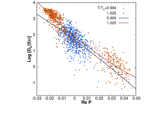
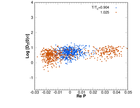
Figure 2: Correlation between the longitudinal (left) and transverse (right) gluon propagator at zero momentum and the real part of the Polyakov loop.

We prove this relying on a procedure analogous to that used in the case of asymmetry. Namely, we also begin with the conditional distribution of the propagator values and find the average value of the propagator as a function of the Polyakov loop using a linear regression model. An important difference from the case of asymmetry is that homoscedasticity of conditional distributions in $D_{L}(0)$ at various values of $\cal P$ is severely broken. The heteroscedasticity is so great that it can hardly be evaluated on the basis of our limited data set. This stems mainly from non-Gaussian character of the distribution of configurations in $D_{L}(0)$, which also holds for the conditional distributions at fixed ${\cal P}$. To obviate this problem, we consider the quantity

$${\cal D}=\ln\big{(}D_{L}(0)\sigma\big{)}$$ (20)

such that the conditional distributions of configurations in it are normal (at least approximately) and the heteroscedasticity can be evaluated. Having such evaluation, we find the conditional average

$$\langle{\cal D}\rangle_{\cal P}\equiv E({\cal D}|{\cal P})=\int{dF({\cal D}|{\cal P})\over d{{\cal D}}}\;{\cal D}d{\cal D}\;,$$ (21)

where $F({\cal D}|{\cal P})$ is the cumulative distribution function of ${\cal D}$ at a given value of the Polyakov loop ${\cal P}$. For this purpose, we employ the linear regression model based on the fit function

$${\cal D}\simeq{\cal D}_{0}(\tau)+{\cal D}_{1}(\tau)\operatorname{Re}{\cal P}(\tau)+{\cal D}_{2}(\tau)\big{(}\operatorname{Re}{\cal P}(\tau)\big{)}^{2}.$$ (22)

The results of our analysis are presented in Table 3. Over the range $-0.1<\tau<0.1$ variation of ${\cal D}(\tau)$ caused by the change of the coefficients ${\cal D}_{0}$ and ${\cal D}_{1}$ is much smaller than the variation caused by the change of ${\cal P}$ according to formula (22), whereas the coefficient ${\cal D}_{2}$ is poorly determined on our statistics. Residuals show correlation with neither $\operatorname{Re}{\cal P}$ nor $\operatorname{Im}{\cal P}$ indicating that $D_{L}(0)$ does not depend on $\operatorname{Im}{\cal P}$ and, within precision available on our data, its dependence on $\operatorname{Re}{\cal P}$ is accounted for by formula (22) with the coefficients from Table 3.

In Maas et al. (2012) it was concluded on the basis of simulations on the $34^{3}\times 4$ lattice that a pronounced jump of the longitudinal propagator is formed at the transition, however, it is not clear whether this discontinuity survives the infinite-volume limit. We argue that such jump can be caused by the difference of the average values of the longitudinal propagator in different Polyakov-loop sectors. In a sufficiently small volume, this difference may be substantial even at $T<T_{c}$ (see next subsection for more detail); therewith, in a finite volume the center symmetry is not broken and no discontinuities in the propagator should emerge. Nevertheless, one can see a discontinuity in the temperature dependence of the propagator even on a small-size lattice at any given temperature $T_{fake}$ provided that one takes into account all three Polyakov-loop sectors at $T<T_{fake}$ and only one Polyakov-loop sector at $T>T_{fake}$. Obviously, such a jump is unrelated to the phase transition. The proper jump of the longitudinal propagator should appear only in the infinite-volume limit and we argue that such a jump does emerge.

$\tau$	${\cal D}_{0}\pm\delta_{STAT}\pm\delta_{SYST}$	${\cal D}_{1}\pm\delta_{STAT}\pm\delta_{SYST}$	${\cal D}_{2}\pm\delta_{STAT}\pm\delta_{SYST}$
-0.096	$1.692\pm 0.024\pm 0.002$	$-56.2\pm 3.5\pm 0.1$	$-94\pm 374\pm 10$
-0.026	$1.753\pm 0.026\pm 0.001$	$-66.7\pm 1.9\pm 0.5$	$293\pm 108\pm 11$
0.025	$1.926\pm 0.038\pm 0.026$	$-64.4\pm 1.2\pm 2.4$	$262\pm 87\pm 40$
0.104	$2.240\pm 0.044\pm 0.178$	$-51.4\pm 1.0\pm 4.0$	$-157\pm 42\pm 95$

Table 3: Results of the fit (22). For each coefficient we present both the statistical error $\delta_{STAT}$ and the systematic error $\delta_{SYST}$ associated with different methods of evaluation of the heteroscedasticity.

Our reasoning is based on

• smooth dependence of the quantity $\langle{\cal D}\rangle_{\cal P}$ (and, therefore, $D_{L}(0)$) on the Polyakov loop

• the fact that, in the infinite-volume limit, the distribution in ${\cal P}$ becomes infinitely narrow (the Polyakov-loop susceptibility tends to infinity as $V\to\infty$);

• the assumption that the coefficients ${\cal D}_{i}$ in formula (22) depend on the lattice size only weakly (this does occur in the $SU(2)$ gluodynamics, however, should be verified in the $SU(3)$ case).

Thus regression analysis gives some evidence that the dependence of ${\cal D}$ (and, therefore, of $D_{L}(0)$) on ${\cal P}$ near the criticality is rather smooth and it is reasonable to draw some consequences of this. Having regard to the fact that, in the infinite-volume limit, the Polyakov loop is a discontinuous function of the temperature, we conclude that the zero-momentum longitudinal gluon propagator is also discontinuous.

It should be noted that the quantity $\displaystyle{\exp\big{(}\langle{\cal D}\rangle\big{)}\over\sigma}$ gives a biased estimate of $\langle D_{L}(0)\rangle$. However, here we focus only on qualitative reasoning and it is sufficient for our purposes that this bias can in principle be evaluated and smooth dependence of $\langle{\cal D}\rangle_{\cal P}$ on ${\cal P}$ implies smoothness of $\langle D_{L}(0)\rangle_{\cal P}$.

Here one should make a comment on the temperature dependence of the zero-momentum longitudinal propagator shown in the left panel of Fig.2 in Ref.Aouane et al. (2012), where it is seen that $D_{L}(0)$ increases with temperature at $0<T<T_{x}$ and approaches its peak at some $T_{x}$ such that $T_{x}<T_{c}$. When $|\tau|\sim 1$, this growth is unrelated to the correlation with the Polyakov loop because the values of ${\cal P}$ are distributed close to zero and we ignore a reason of such growth. However, at subcritical temperatures ($\tau<0,\ |\tau|<\!\!\!<1$) the width of the $|{\cal P}|$ distribution begins to rise. It should be emphasized that, at a nonvanishing width of the $|{\cal P}|$ distribution, $D_{L}(0)$ depends substantially on which Polyakov-loop sectors are taken into consideration.

Since only sector ($I$) was taken into account in Ref.Aouane et al. (2012), the correlation shown in Fig.2 indicates that a broadening of the $|{\cal P}|$ distribution results in a decrease of $D_{L}(0)$. However, in another Polyakov-loop sector, $D_{L}(0)$ increases with broadening of the $|{\cal P}|$ distribution. When all three sectors are taken into consideration, $D_{L}(0)$ continues to increase up to $T=T_{c}$ and decreasing of $D_{L}(0)$ with temperature at $T>T_{c}$ occurs only due to the restriction to sector $(I)$.

In a finite volume both the Polyakov loop and the propagator are smooth functions of $T$. However, when one takes an average $\langle D_{L}(0)\rangle$ over configurations in all three sectors at $T<T_{c}$ and over configurations only in sector $(I)$ at $T>T_{c}$, the above reasoning implies that such an average jumps down at $T=T_{c}$ and this is a fake discontinuity associated with an abrupt artificial restriction to only one sector: it is precisely what was shown in Maas et al. (2012). Such restriction is justified only in the infinite-volume limit.

In this limit, $D_{L}(0)$ jumps precisely at $T=T_{c}$ exactly opposite to the Polyakov loop: it jumps down provided that sector $I$ is chosen by the system at $T>T_{c}$ and jumps up when the system at $T>T_{c}$ chooses sector $II$ or $III$.

In any case, for a comprehensive investigation of the critical behavior of Green functions all Polyakov-loop sectors should be taken into account in some neighborhood of the critical temperature.

IV.1 Propagators in different Polyakov-loop sectors

Our statistics is not sufficient for a detailed study of the gluon propagators at a given value of the Polyakov loop or, more precisely, at a given value of $\operatorname{Re}{\cal P}$ since they are independent of $\operatorname{Im}{\cal P}$. However, certain conclusions on the behavior of the propagators below and above $T_{c}$ can be drawn simply from considering them in different Polyakov-loop sectors. Since the propagators computed in sector ($II$) coincide with those in sector ($III$), we compare the propagators evaluated in sector ($I$) referred to as “Re ${\cal P}>0$” with those evaluated on configurations from sectors ($II$) and ($III$) referred to as “Re ${\cal P}<0$”.

We begin with a comparison of zero-momentum values of the propagators presented in Table 4. In addition to the rapid decrease with increasing Polyakov loop shown in the left panel of Fig.2, it is clearly seen in Table 4 that the zero-momentum longitudinal propagator decreases with temperature at Re ${\cal P}>0$ and increases with temperature at Re ${\cal P}<0$. For the lattice size under consideration ($\sim 2$ fm) the ratio

$$j={D_{L}^{\operatorname{Re}{\cal P}<0}(0)\over D_{L}^{\operatorname{Re}{\cal P}>0}(0)}$$

runs up to 3 well below the critical temperature ($\tau=-0.026$). Above the critical temperature, $j$ shows a rapid growth and reaches 30 at $\tau\approx 0.1$.

$\tau$	$D_{L}(0)$	$D_{L}(0)$	$D_{T}(0)$	$D_{T}(0)$
	$\operatorname{Re}{\cal P}>0$	$\operatorname{Re}{\cal P}<0$	$\operatorname{Re}{\cal P}>0$	$\operatorname{Re}{\cal P}<0$
-0.096	20.88(65)	36.16(1.17)	9.36(14)	8.79(12)
-0.026	17.7(1.3)	54.97(1.93)	9.19(16)	8.35(12)
0.025	8.82(1.22)	99.35(2.11)	9.44(14)	7.57(11)
0.104	3.95(16)	125.53(1.38)	9.30(15)	6.68(10)

Table 4: Average values of the zero-momentum propagators in different Polyakov-loop sectors. No difference between sectors ($II$) and ($III$) has been found, they are referred to as “$\operatorname{Re}{\cal P}<0$”.

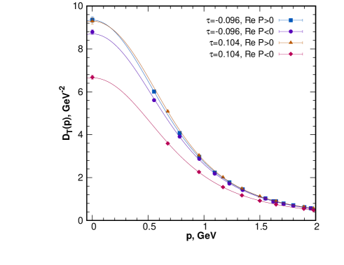
Figure 3: Longitudinal (left) and transverse (right) gluon propagator as functions of the momentum in different Polyakov-loop sectors below and above critical temperature. Notice logarithmic scale on the ordinate axis on the left panel.

Both in the right panel of Fig.2 and in Table 4 it is demonstrated that, in contrast to the longitudinal propagator, the zero-momentum transverse propagator slightly increases with an increase of the Polyakov loop. Within statistical errors, it does not change with temperature at Re ${\cal P}>0$ and shows moderate decreasing at Re ${\cal P}<0$.

The propagators at momenta $p<2.2$ GeV for different Polyakov-loop sectors are shown in Fig.3.

The curves in Fig.3 are the results of the fit based on the Gribov-Stingl formula

$$D(p)\simeq c{p^{2}+d^{2}\over(p^{2}+M^{2})^{2}+b^{4}}$$ (23)

over the momentum range $p<2.5$ GeV, here we only mention that it works well. The transverse propagator shown in the right panel shows a noticeable difference

$$\mathbf{d}_{T}(p)=D_{T}^{\operatorname{Re}{\cal P}<0}(p)-D_{T}^{\operatorname{Re}{\cal P}>0}(p)$$

which rapidly decreases with increasing momentum and moderately increases with increasing temperature. This being so, the transverse propagator is independent of temperature in the sector $\operatorname{Re}{\cal P}>0$ and is decreasing with temperature in the sector $\operatorname{Re}{\cal P}<0$.

As compared with the transverse propagator, the longitudinal propagator features a huge difference

$$\mathbf{d}_{L}(p)=D_{L}^{\operatorname{Re}{\cal P}<0}(p)-D_{L}^{\operatorname{Re}{\cal P}>0}(p)$$

in a deep infrared, which is, however, characterized by a very sharp decrease with the momentum, especially at $\tau>0$. Though $\mathbf{d}_{L}(p)$ increases with increasing temperature, the behavior of the longitudinal propagator by itself is more complicated. In the sector $\operatorname{Re}{\cal P}>0$, the longitudinal propagator substantially decreases with increasing temperature over the range $-0.1<\tau<0.1$, whereas in the sector $\operatorname{Re}{\cal P}<0$ it decreases with increasing temperature only at $p\gtrsim 0.4$ GeV; at smaller momenta it rapidly increases over the range $-0.1<\tau<0.1$.

IV.2 Screening masses

We also evaluate screening for different sectors of the Polyakov loop. The chromoelectric and chromomagnetic screening masses are obtained from the fit of the formula

$${1\over D_{L,T}(p)}\simeq{1\over Z}\left(m_{E,M}^{2}+p^{2}+rp^{4}\right)$$ (24)

to the data on inverse longitudinal and transverse gluon propagators at low momenta, respectively; for more detail about this definition of screening masses see Refs.Bornyakov et al. (2020a, b). We performed fit over the range $0\leq p<1.3$  GeV, in this domain the fit formula (24) works well for both the longitudinal and the transverse propagators giving a reliable fit quality for all Polyakov-loop sectors. The fit is stable with respect to variations of the upper bound of the fit range between 1.2 and 1.6 GeV and to an exclusion of zero momentum. The results for screening masses are presented in Table 5.

Chromomagnetic screening masses in different Polyakov-loop sectors differ slightly, if at all, and their temperature dependence is not clearly seen. For this reason we take a closer look at chromoelectric sector and consider $m_{E}$ and $D_{L}(0)$ relative to their chromomagnetic counterparts.

$\tau$	$m_{E}^{2}$	$m_{E}^{2}$	$m_{M}^{2}$	$m_{M}^{2}$
	$\operatorname{Re}{\cal P}>0$	$\operatorname{Re}{\cal P}<0$	$\operatorname{Re}{\cal P}>0$	$\operatorname{Re}{\cal P}<0$
-0.096	0.373(31)	0.214(31)	0.638(34)	0.642(39)
-0.026	0.445(71)	0.136(11)	0.609(24)	0.586(32)
0.025	0.523(56)	0.0498(38)	0.672(37)	0.565(18)
0.104	0.95(20)	0.0272(11)	0.664(43)	0.611(8)

Table 5: Values of the chromoelectric and chromomagnetic screening masses (in GeV²) obtained by the fit formula (24) in different Polyakov-loop sectors. No difference between sectors ($II$) and ($III$) has been found, they are referred to as “$\operatorname{Re}{\cal P}<0$”.

As $T/T_{c}$ increases from 0.9 to 1.1, the chromoelectric screening mass in the sector $\operatorname{Re}{\cal P}<0$ increases from 600 MeV to 1 GeV, whereas in the sector $\operatorname{Re}{\cal P}<0$ it decreases from 460 MeV to 160 MeV. The difference between the screening masses in different Polyakov-loop sectors at $T<T_{c}$ can be attributed to finite-volume effects related to a finite width of the distribution in $\operatorname{Re}{\cal P}$. In the deconfinement phase screening of color charges is different in different sectors. At $T=1.1T_{c}$, as an example, screening radii differ substantially: 1.2 fm in the sector $\operatorname{Re}{\cal P}>0$ versus 0.2 fm in the sector $\operatorname{Re}{\cal P}<0$.

It was shown in Bornyakov and Rogalyov (2021) that, when the screening mass is sufficiently large, the strength of chromoelectric or chromomagnetic interactions between static color charges or currents should be characterized by the quantity

$$V_{E}=m_{E}^{3}D_{L}(0)\qquad\mbox{or}\qquad V_{M}=m_{M}^{3}D_{T}(0)$$ (25)

rather than by $D_{L}(0)$ or $D_{T}(0)$, respectively. The screening masses in the case under consideration are rather small, nevertheless, in Table 6 we present the values of $V_{E,M}$ which have the meaning of the depth of the static-quark potential well in the limit of large screening masses. Though these quantities are normalization dependent, their ratios give information, in particular, on the strength of chromoelectric interactions relative to the strength of the chromomagnetic interactions in different Polyakov-loop sectors.

As the temperature increases from $0.9T_{c}$ to $1.1T_{c}$, the ratio $\displaystyle\left.{V_{E}\over V_{M}}\right|_{\operatorname{Re}{\cal P}>0}$ decreases by some 30% and the ratio $\displaystyle\left.{V_{E}\over V_{M}}\right|_{\operatorname{Re}{\cal P}<0}$ decreases more than by a factor of four.

$\tau$	$V_{E}$, GeV		$V_{M}$, GeV
	$\operatorname{Re}{\cal P}>0$	$\operatorname{Re}{\cal P}<0$	$\operatorname{Re}{\cal P}>0$	$\operatorname{Re}{\cal P}<0$
-0.096	4.8	3.5	4.8	4.5
-0.026	5.2	2.8	4.4	3.7
0.025	3.3	1.1	5.2	3.2
0.104	3.7	0.56	5.0	3.2

Table 6: Strength of the chromoelectric ($V_{E}$) and chromomagnetic ($V_{M}$) interactions determined by formula (25) in different Polyakov-loop sectors. Errors are not shown because the presented values can be used only for rough qualitative estimates.

Thus in the deconfinement phase the relative strength of chromoelectric interactions decreases slightly in the sector $\operatorname{Re}{\cal P}>0$ and significantly in the sector $\operatorname{Re}{\cal P}<0$. This being so, the chromoelectric screening radius decreases in the sector $\operatorname{Re}{\cal P}>0$ both in absolute value and with respect to the chromomagnetic screening radius and dramatically increases in the sector $\operatorname{Re}{\cal P}<0$.

Gluon matter in the deconfinement phase can be considered as chromomagnetic medium, that is, as a medium with weaken and well-screened chromoelectric interactions provided that the the sector $\operatorname{Re}{\cal P}>0$ is chosen. Choosing one of the sectors with $\operatorname{Re}{\cal P}<0$, we arrive at a medium with strong and short-range chromomagnetic interactions and weak and long-range chromoelectric interactions.

IV.3 Speculations on the deconfinement phase transition

Thus the longitudinal propagator in the sector $\operatorname{Re}{\cal P}>0$ differs dramatically from the longitudinal propagator in the sector $\operatorname{Re}{\cal P}<0$. In this connection, it is reasonable to recollect the confinement scenario proposed, in particular, in Refs.Fortunato and Satz (2000); Gattringer and Schmidt (2011) and investigated in Ivanytskyi et al. (2017). In these works, the properties of the gluon medium responsible for confinement of heavy static quarks were discussed. Such medium can be characterized in terms of center clusters (the domains where the Polyakov loop takes the values mainly from one sector).

In the deconfinement phase, there exists a percolating cluster associated with some center element of the gauge group, and the remaining space is either occupied by finite-size clusters associated with some center element or characterized by the values of the Polyakov loop that does not clearly favor a definite center element. As the temperature decreases, the part of space occupied by the percolating cluster decreases until it disappears at the critical temperature.

Let us proceed to some qualitative speculations to outline directions of further investigations. Our finding that the Polyakov-loop sectors differ in the infrared behavior of the longitudinal gluon propagator gives some evidence that static color charges interact differently in different clusters. Thus the Polyakov-loop sectors are not equivalent for gauge-dependent quantities even in a pure gauge theory. In the Landau gauge, we obtain that the “trivial” sector $\operatorname{Re}{\cal P}>0$ is preferred in the sense that it features the most screened chromoelectric interaction between color static charges. This is the most natural choice of the Polyakov-loop value in the deconfinement phase. In the Landau gauge, the finite-size clusters associated with the other center elements $\operatorname{Re}{\cal P}<0$ can be considered as “bubbles of glue” in the deconfinement phase: in the Landau gauge, the longitudinal gluon propagator provides long-range chromoelectric interaction of static color charges within such clusters. Their volume increases with decreasing temperature, whereas the range of color-charge interaction within each such cluster decreases. In a percolating cluster, the opposite happens. Its volume decreases with decreasing temperature, whereas the range of chromoelectric forces increases. At the critical temperature all clusters become identical (in the infinite-volume limit).

Such a scenario should be checked in further lattice simulations; in particular, the color-singlet and color-octet potentials in each Polyakov-loop sector should be studied. Another problem is to study the high-temperature behavior of the differences $\mathbf{d}_{L}(p)$ and $\mathbf{d}_{T}(p)$ which rapidly decrease with increasing momentum. It is interesting to find out whether there really is a momentum $p_{J}$, common to all temperatures, such that both $\mathbf{d}_{L}(p)$ and $\mathbf{d}_{T}(p)$ become negligible at $p>p_{J}$. Such a momentum would indicate the boundary between nonperturbative infrared and perturbative ultraviolet domains in gluodynamics.

V Conclusions

We have studied the asymmetry ${\cal A}$ and the longitudinal gluon propagator in the Landau-gauge $SU(3)$ gluodynamics on lattices $24^{3}\times 8$ over the range of temperatures $0.9T_{c}<T<1.1T_{c}$. Our findings can be summarized as follows:

• Both the asymmetry ${\cal A}$ and the zero-momentum longitudinal propagator $D_{L}(0)$ have a significant correlation with the real part of the Polyakov loop ${\cal P}$. The correlation between $D_{T}(0)$ and $\operatorname{Re}{\cal P}$ is non-negligible. Neither ${\cal A}$ nor $D_{L}(0)$ nor $D_{T}(0)$ has a correlation with $\operatorname{Im}{\cal P}$.

• We suggest a method to substantially reduce finite-volume effects. In the deconfinement phase, the conditional averages $\langle{\cal A}\rangle_{{\cal P}=z}$ or $\langle D_{L}(0)\rangle_{{\cal P}=z}$ give a close approximation to the infinite-volume limit of ${\cal A}$ or $D_{L}(0)$ at the temperature $\tau$ determined from the equation ${\cal P}_{\infty}(\tau)=z$ provided that $z$ is an allowed infinite-volume value of the Polyakov loop in a chosen sector and ${\cal P}_{\infty}$ is the infinite-volume expectation value of ${\cal P}$.

• We determined critical behavior of ${\cal A}$ and $D_{L}(0)$ in the infinite-volume limit. Regression analysis reveals that the conditional averages $\langle{\cal A}\rangle_{\cal P}$ and $\langle D_{L}(0)\rangle_{\cal P}$ are smooth functions of the Polyakov loop. Discontinuity in the Polyakov loop at $T=T_{c}$ in the infinite-volume limit implies discontinuity of the asymmetry and the longitudinal gluon propagator. The discontinuities of ${\cal A}$ and $D_{L}(0)$ at $T=T_{c}$ are readily determined from the dependencies of $\langle{\cal A}\rangle_{\cal P}$ and $\langle D_{L}(0)\rangle_{\cal P}$ on $\operatorname{Re}\!{\cal P}$.

• The infrared behavior of the longitudinal propagator depends significantly on the Polyakov-loop sector; a moderate dependence of the transverse propagator in the infrared on the Polyakov-loop sector is also observed.

• In the deconfinement phase, distinctions between gauge-dependent quantities in different Polyakov-loop sectors are significant. We have considered as an example chromoelectric interactions relative to chromomagnetic interactions, whose dependence on the temperature and the Polyakov-loop sector is not very significant. They are weakly suppressed and short-range in the sector $\operatorname{Re}\!{\cal P}>0$ and moderately suppressed and long-range in each sector with $\operatorname{Re}\!{\cal P}<0$.