A Spatial-Temporal asymptotic preserving scheme for radiation magnetohydrodynamics in the equilibrium and non-equilibrium diffusion limit
Abstract.
The radiation magnetohydrodynamics (RMHD) system couples the ideal magnetohydrodynamics equations with a gray radiation transfer equation. The main challenge is that the radiation travels at the speed of light while the magnetohydrodynamics changes with the time scale of the fluid. The time scales of these two processes can vary dramatically. In order to use mesh sizes and time steps that are independent of the speed of light, asymptotic preserving (AP) schemes in both space and time are desired. In this paper, we develop an AP scheme in both space and time for the RMHD system. Two different scalings are considered. One results in an equilibrium diffusion limit system, while the other results in a non-equilibrium system. The main idea is to decompose the radiative intensity into three parts, each part is treated differently with suitable combinations of explicit and implicit discretizations guaranteeing the favorable stability conditionand computational efficiency. The performance of the AP method is presented, for both optically thin and thick regions, as well as for the radiative shock problem.
1. Introduction
Radiation magnetohydrodynamics (RMHD) is concerned with the dynamical behavior of magnetized fluids that have nonnegligible exchange of energy and momentum with radiation, which is important in high temperature flow systems, solar and space physics and astrophysics. The radiation transfer equation (RTE) for the radiative intensity and the fluid temperature in the mixed frame (the radiative intensity is described in an Eulerian frame while the material coupling terms are described in the comoving frame) is governed by
| (1.1) | ||||
where and represent absorption and scattering opacities respectively, is the angular variable, is the radiation constant and is the speed of light [pub.1041264084]. , are the zeroth, first, second angular moments of , respectively:
The ideal MHD equations with radiation energy and momentum source terms are
| (1.2) |
where
with the energy density
the radiation flux
and the radiation pressure
In particular, the operators and are respectively , and in this context. Moreover, is the fluid density; is the fluid velocity; is the magnetic flux density; is the static pressure; (with the identity matrix) is the full pressure tensor of the fluid; is the full pressure of the fluid;
where is the internal energy density; and . The radiation MHD system is closed by the perfect gas equation of state:
where is adiabatic index for an ideal gas, and is the ideal gas constant.
Numerical approximations to the RTE have been extensively studied in [MCCLARREN20087561, MOREL1996445, sun2015asymptotic, jin2009uniformly, KFJ16, klar1998asymptotic] and for ideal MHD see for example [stone2008athena, brio1988upwind, li2011central]. The RMHD coupled system has been investigated lately [pub.1005319601, BOLDING2017511, SEKORA20106819, KADIOGLU20108313, pub.1041264084, sekora2009higher, sun2020multiscale]. Since the transport term in the RTE and the advection term in the MHD equations are at different time scales, the RMHD system can be stiff, as can been seen more clearly after nondimensionalization [lowrie1999coupling]. To solve the RMHD system, classical numerical discretizations require the space and time steps to resolve the speed of light, which is very expensive. Asymptotic-Preserving (AP) schemes provide a generic framework for such multiscale problems [jin1999efficient, JinReview]. AP schemes were first studied for steady neutron transport problems in diffusive regimes [larsen1987asymptotic, larsen1989asymptotic] and then [golse1999convergence, 2018Tang] for boundary value problems, unsteady transport problems [jin1998diffusive, klar1998asymptotic] and gray radiative transport equations [2001Klar, 2021Tang]. When the scaling parameter in the multiscale system can not be resolved numerically, AP schemes should automatically become a good solver for the macroscopic models.
AP schemes for RMHD have been proposed in the literature, but since most of them are based on operator splitting, they are only AP in space. In [BOLDING2017511], Simon et al. have developed a second-order scheme in both space and time for the Euler equations coupled with a gray radiation model. The scheme in [BOLDING2017511] uses MUSCL-Hancock method to solve the Euler equations and the lumped linear-discontinuous Galerkin method for the radiation model. For the time discretization, the TR/BDF2 time integration method is employed. Jiang et al. devised an Implicit/Explicit (IMEX) scheme for the splitting system that treats the transport term in the RTE and convective term in the fluid equations explicitly, and the source term implicitly [pub.1041264084]. Recently, another method by Sun et al. [sun2020multiscale] solves a coupled system of RTE and Euler equations, the authors use the gas-kinetic scheme (GKS) to solve the Euler equations and disretize the RTE by the unified gas-kinetic scheme (UGKS). However, all the aforementioned methods either require a time step that satisfies a hyperbolic constraint with CFL number proportional to the speed of light [sun2020multiscale], or use nonlinear iterations involving (1.1) in order to get rid of the time step constraint [BOLDING2017511, pub.1041264084]. Both approaches are expensive. It is desired to design a scheme that can use a time step that is independent of the speed of light and employs nonlinear iterations that involve only macroscopic quantities, i.e. the , , , or the moments of radiative intensity.
In this paper, we aim at developing a scheme for RMHD that is AP in space time. Two different parameter regimes are considered. One is for small and large, which results in the non-equilibrium diffusion limit system. The other is for large, which gives the equilibrium diffusion limit system. The proposed scheme preserves both limits. The main idea is to decompose the intensity into three parts, two parts correspond to the zeroth and first order moments, while the third part is the residual. The two macroscopic moments are treated implicitly while the residual is explicit. Thanks to the properties of the residual term, one can update the macroscopic quantities first. The residual term is then updated by solving implicitly a linear transport equation for each direction . For the space discretization, we use Roe’s method in the Athena code to solve the convective part in the ideal MHD equations and the UGKS for the RTE. AP property of both semi-discretized and fully discretizad systems are proved.
The computational cost of our proposed scheme is lower due to the following reasons. Compared to the explicit scheme, much larger time steps are allowed. On the other hand, compared to the fully implicit scheme, our scheme requires nonlinear iterations to solve a system with only macroscopic quantities and then one linear transport equation for each direction . Since different directions are decoupled, the computational cost is much lower than solving implicitly a linear RTE where all velocities are coupled. The computational bottleneck due to the resolution of the angular dimension is avoided.
This paper is organized as follows. Section 2 gives the asymptotic limit of the coupled system, and the equilibrium and non-equilibrium diffusion limit systems under different scalings are obtained. The semi-discretization and one dimensional fully discretized scheme for RMHD are illustrated in Sections 3 and 4 respectively. Their capability of capturing both diffusion limits are proved. In Section 5, the performance of our AP method is presented in both optically thin and thick regions. The radiative shock problems are tested. By comparing with the semi-analytic solutions from [lowrie2008radiative], we observe that the scheme is accurate and stable using large time step and meshes that are independent of the speed of light. Finally, we conclude in Section 6.
2. The diffusion limit of RMHD
As presented in [lowrie1999coupling], the dimensionless form for the coupled system can give a better insight on the relative importance of different terms. Consider the following nondimensionalization:
where variables with a hat denote nondimensional quantities and variables with subscript are the characteristic values with units. More precisely, , , and are respectively the reference length, sound speed, density and temperature. Moreover, and are respectively the characteristic values of absorption and scattering coefficients. Then the full dimensionless radiation MHD system becomes (after dropping the hat):
| (2.1) |
where , , , , and . In (2.1), is a nondimensional constant, which measures the influence of radiation on the flow dynamics. In [godillon2005coupled, BCDB1, BCDB2], the authors derived the equilibrium diffusion and non-equilibrium diffusion limits for a system that is composed of a kinetic equation and a drift-diffusion equation or Euler equations. In [lowrie1999coupling], the authors considered four different regimes for the RMHD system: equilibrium diffusion regime, strong equilibrium regime, isothermal regime and streaming regime. In the subsequent part, we will focus on two regimes of the RMHD system: equilibrium diffusion and non-equilibrium diffusion limit regimes, whose derivations are the same as in [godillon2005coupled, BCDB1, BCDB2, lowrie1999coupling]. For the convenience of readers, the details of the derivation are in Appendix A.
2.1. The non-equilibrium diffusion limit.
In this regime the radiation intensity tends to a state which can be characterized by a temperature which is different from the material temperature . As in the reference, we consider the following scaling
Here the introduction of is for the convenience of asymptotic analysis, and the value of depends on the speed of light. The RMHD system (2.1) becomes:
| (2.2a) | |||||
| (2.2b) | |||||
| (2.2c) | |||||
| (2.2d) | |||||
| (2.2e) | |||||
where
When in (2.2), the solution can be approximated by the solution of the following non-equilibrium system:
| (2.3a) | |||||
| (2.3b) | |||||
| (2.3c) | |||||
| (2.3d) | |||||
| (2.3e) | |||||
Here, the non-equilibrium system indicates that is away from , while we will see in section 2.2 that the equilibrium diffusion limit indicates that .
2.2. The equilibrium diffusion limit.
In this regime the radiation intensity adapt to the material temperature. As in the reference, we consider the following scaling
This is called the equilibrium diffusion regime, which will give the classical equilibrium diffusion limit [pomraning2005equations, mihalas1984foundations, lowrie1999coupling]. The RMHD system (2.1) becomes:
| (2.4a) | |||||
| (2.4b) | |||||
| (2.4c) | |||||
| (2.4d) | |||||
| (2.4e) | |||||
where
When in (2.4), the solution can be approximated by the solution of the following equilibrium system:
| (2.5a) | |||||
| (2.5b) | |||||
| (2.5c) | |||||
| (2.5d) | |||||
As we can see, when in (2.3), the non-equilibrium diffusion system (2.3) is the same as the equilibrium diffusion system (2.5), which indicates is close to in the equilibrium system (2.4).
Remark 1.
To understand the above scalings, we choose the light speed, the characteristic material temperature and the radiation constant to be respectively (), and . The typical computational domain is 0.04 , and the units of the length, time, temperature and energy are respectively and (). For the above parameters, we can choose . Then, when , , the parameters are in the non-equilibrium diffusion regime and when , , in the equilibrium diffusion regime.
3. Time discretization for the RMHD
In this section, based on a decomposition for radiation intensity , we will present a semi-discretization for the RMHD and show its AP property for any dimensions in space and angular variables.
3.1. A decomposition
To preserve the asymptotic limit of (2.1), the main idea is to decompose the intensity into three parts, and each of them is treated in a different way. More precisely, we decompose as follows:
| (3.1a) | |||
| (3.1b) |
where 3. Then taking on both sides of (3.1a) yields
which gives
| (3.2) |
Moreover, taking on (3.1b), yields
which implies
| (3.3) |
The idea is close to the micro-macro decomposition in [klar1998asymptotic, LM]. However, we do not write down the macroscopic and microscopic equations explicitly, which is different from the classical micro-macro decomposition method as in [klar1998asymptotic].
Substituting the decomposition (3.1) into system (2.1) leads to
| (3.4a) | |||||
| (3.4b) | |||||
| (3.4c) | |||||
| (3.4d) | |||||
| (3.4e) | |||||
where ( denotes the 3 by 3 identity matrix), and
(3.4a) has three unknown functions, and . Thanks to the properties of in (3.2),(3.3), the zeroth and first moment equations of (3.4a) have no time derivatives with respect to . Therefore, instead of solving the RMHD system (3.4) directly, we take the zeroth and first moments of (3.4a), and then couple them together with (3.4b)–(3.4e) to solve variables . More precisely, we have
| (3.5) |
coupled with (3.4b)–(3.4e) and by treating explicitly, one can update the macroscopic quantities first. Then can be updated implicitly, and the new can be given by (3.1). The details are illustrated in the next two subsections.
3.2. The time discretization for (2.1)
Let
and
We use the following semi-discrete scheme in time for (3.4), which reads:
| (3.6a) | |||||
| (3.6b) | |||||
| (3.6c) | |||||
| (3.6d) | |||||
| (3.6e) | |||||
where and
The zeroth and first moment equations of (3.6a) are
The non-equilibrium diffusion limit of (3.6):
In the non-equilibrium regime, the scalings of the coefficients are
Then we will show the AP property of the semi-discretization (3.7) in the non-equilibrium regime. By using Champan-Enskog expansion in equation (3.8), one can get
| (3.9) | ||||
which indicates
The residual term at current step can be gotten by equation (3.8), then one can get
| (3.10) |
From (3.7b),
| (3.11) |
by using equation (3.10), equation (3.11) reduces to
| (3.12) |
Multiplying equation (3.7a) by , and adding it up with equation (3.6d), we get
| (3.13) | ||||
By using (3.12), and sending in equation (3.13) yields
| (3.14) | ||||
This is a semi-discretization for (2.3c). Then multiplying equation (3.7b) by , and adding it to equation (3.6c), sending , formally one gets
| (3.15) |
This is a semi-discretization for (2.3b). Sending in equation (3.7a), yields
| (3.16) |
which is a semi-discretization (2.3d).
The equilibrium diffusion limit of (3.6):
In the non-equilibrium regime, the scalings of the coefficients are
The derivation of the equilibrium diffusion limit is similar to the non-equilibrium case, but requires additional analysis for the zeroth moment of equation (3.6a). Sending in the zeroth moment equation of (3.6a), one gets
which implies
Therefore, (3.14) and (3.15) in the equilibrium regime become
4. The full discretization for the non-equilibrium regime
For the ease of exposition, we will explain our spatial discretion in 1D. That is, , , and . Recall the RMHD equations in slab geometry:
| (4.1a) | |||||
| (4.1b) | |||||
| (4.1c) | |||||
| (4.1d) | |||||
| (4.1e) | |||||
| (4.1f) | |||||
| (4.1g) | |||||
| (4.1h) | |||||
where
and and are fluid velocity in the , , and directions, respectively. and are magnetic field in the , , and directions, respectively. The boundary condition becomes
| (4.2) |
Higher dimensions can be treated in the dimension by dimension manner. Let be the computational domain, , and we consider the uniform mesh as follows
and let
To get a consistent stencil in spatial discretization, we use the unified gas kinetic scheme (UGKS) for spatial discretization [mieussens2013asymptotic]. Other space discretization that is AP can be applied as well. The most crucial point is that the space discretization of the MHD system has to be consistent with that of the RTE.
4.1. A finite volume approach
UGKS is a finite volume method. Integrating the RMHD system (4.1) over and gives
| (4.3a) | |||||
| (4.3b) | |||||
| (4.3c) | |||||
| (4.3d) | |||||
| (4.3e) | |||||
| (4.3f) | |||||
| (4.3g) | |||||
| (4.3h) | |||||
where , and are
Here the numerical fluxes at the interfaces use Roe’s Riemann solver [stone2008athena], based on the piecewise linear reconstruction. At last, we discuss the microscopic flux defined at the interface in (4.3a). In [mieussens2013asymptotic], all the terms of the microscopic flux are treated explicitly, in this paper all the terms except the initial value and are treated , and the processes of UGKS are detailed in Appendix B.
With the expressions (B.3), (B.4) and (B.5), the numerical flux is
| (4.4) | ||||
where is the indicator function. Moreover, the coefficients in the numerical flux are given by:
| (4.5) | ||||
with .
To obtain a scheme that can update the quantities ,, and , the zeroth moment and first moment of velocity field for (4.3a) are needed. Integrating equation (4.3a) for from -1 to 1, and multiplying the both sides by , one can obtain
| (4.6) |
where
Multiplying equation (4.3a) by , then integrating it for from -1 to 1, and multiplying the both sides by , one can obtain
| (4.7) |
where
Coupling equations (4.6), (4.7), (4.3c) and (4.3f) as a system and solving the system, quantities , , and can be updated. Finally, quantity can be updated implicitly by equation (4.3a), which reads
where
and
and the new can be given by using (3.1).
4.2. The diffusion limit of (4.3c)–(4.7)
Firstly, the non-equilibrium regime is considered, i.e.,
Assuming and are positive, as , the leading order of the coefficients in the numerical flux (4.4) are
This means the zero moment and the first moment of the numerical flux, as , have the following limit:
| (4.8) |
| (4.9) |
in which the condition the residual term is the same order with in the non-equilibrium regime has been used.
Multiplying equation (4.6) by , and adding it up with equation (4.3f), the terms on the right hand sides cancel. Sending and using (4.8) yields
| (4.10) | ||||
This is a full discretization for (2.3c). Then multiplying equation (4.7) by , and adding it to equation (4.3c), sending and using (4.9), one obtains
| (4.11) |
This is a full discretization for (2.3b). Sending in equation (4.7) and using (4.9) gives
| (4.12) |
using (4.12) in (4.6) and sending , one gets
| (4.13) |
which is a full discretization for (2.3d). Next, we will give the diffusion limit of the full discretization of the equilibrium case. Firstly, assuming and are positive, as , the leading order of the coefficients in the numerical flux (4.4) are
which means the zeroth moment and the first moment of the numerical flux, as , have the following limit:
| (4.14) |
| (4.15) |
in which the condition the residual term is the same order as in the equilibrium regime has been used. In equation (4.6), letting , one can obtain
Multiplying equation (4.6) by , adding it to the energy equation and substituting limit (4.14) into the equation, then multiplying equation (4.7) by , adding it to the momentum equation and substituting limit (4.15) into the equation, at last letting in the two equations, one can obtain
| (4.16) | ||||
| (4.17) |
4.3. Boundary conditions
In this section, the numerical fluxes in the system (4.3c)–(4.7) under the boundary condition (4.2) are considered. The construction of the flux on the right boundary is similar to the construction on the left boundary, for which we only consider the left boundary case. At the left boundary, the integral representation of the radiative intensity (B.3) reads:
| (4.18) |
According to the approximation (B.4) and (B.5) , the reconstruction of for and at the left boundary can be written as:
and the reconstruction of for in the interval :
where and . Then the numerical flux at the left boundary reads:
which indicates
here is the material temperature at the left boundary, and
To summarize, we have the following one time step update of the fully discrete version of RMHD.
5. Numerical Examples
In this section, we conduct several numerical experiments to test the performance of our proposed method. The Dirichlet boundary conditions are adopted in all the following examples. For velocity discretization, we choose the discrete-ordinate method [SKTS]. In all numerical examples, discrete ordinate method has been used.
The first example is for the RMHD system where the radiation does not effect the fluid i.e. , but the fluid provides a source for radiation. The second example is to illustrate the performance of the radiation solver when both optical thick and thin regions coexist, in which the fluid density , velocity and temperature are fixed. In example 3, a range of radiation-hydrodynamic shock problems are tested. In example 4, using different absorption and scattering coefficients, AP property of the proposed scheme for the full RMHD system is illustrated numerically. Finally, optical thick and thin regions coexisting case are tested in Example 5 and we can see that large time step is allowed.
5.1. Example 1
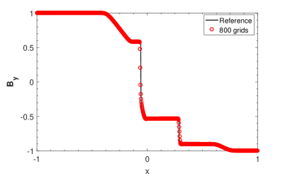
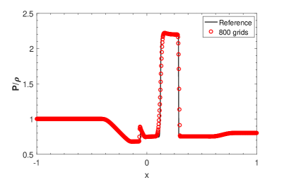
In this example, we will test an ideal MHD shock tube problem as in Section V in [brio1988upwind], where =0 in (2.2). The computational domain is and the initial data is given by
| (5.1) |
The magnetic intensity in the direction , the ideal gas constant and adiabatic index for an ideal gas , the absorption collision cross-section , the scatter collision cross-section , and in the RMHD system (2.2). The exact solutions at time involve two fast rarefaction waves, a slow compound wave, a contact discontinuity, and a slow shock. Fig. 1 displays the numerical solutions at obtained by our method with . The reference solution is computed by Roe’s method shown in [stone2008athena] with with . For all the schemes, the time step is
5.2. Example 2
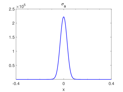
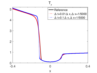
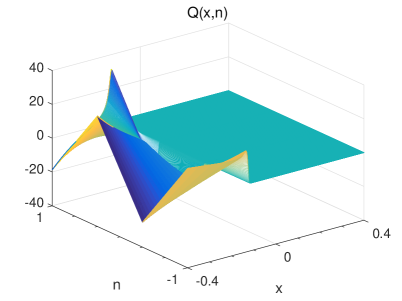
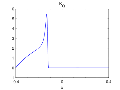
A problem with both optically thick and thin regions is tested for the radiation subsystem. This kind of problems has been studied in [pub.1041264084, pub.1005319601, filbet2010class, hayes], where the gas is held inactive, and only the radiation equation in system (2.1) is evolved, i.e., the evolution of the radiation does not change the gas density and momentum. In this test, a blob of optically thick gas is located in the middle of the computational domain , surrounded by an optically thin gas. The gas density is
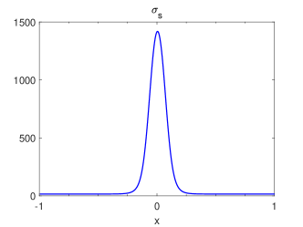
and the gas temperature is adjusted to provide constant pressure in the domain, which is set to be . The initial radiative energy density is at local thermal equilibrium. The boundary condition is set to be and , , and . See Fig. 2(a) for the absorption coefficient, which varies from 1 to . For this example, we compare the radiation temperature obtained by our AP scheme and an explicit solver on a finer mesh in Fig. 2(b). We use the space step for both AP and the explicit solver, but the time step sizes are different such that and for the AP solver and for the explicit solver. The good agreement between our and the reference solution indicates that the AP method works well in the coexistence case. Moreover, we plot in Fig. 2(d), the value of can be as large as in this example. From Fig. 2(b), when at , the radiation was stopped by the opaque material.
5.3. Example 3
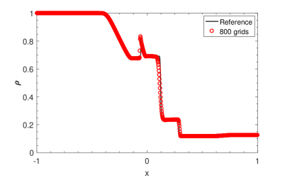
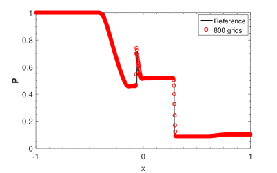
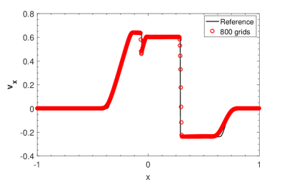
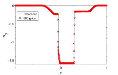
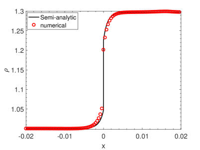
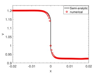
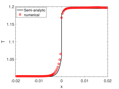
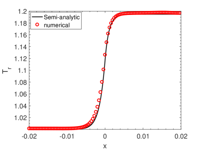
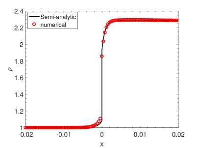
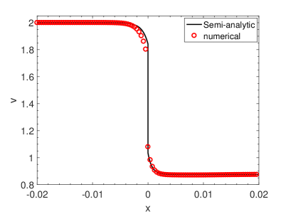
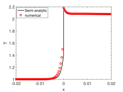
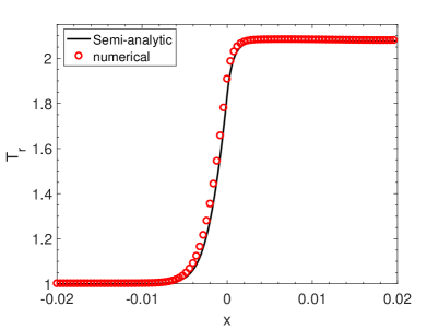
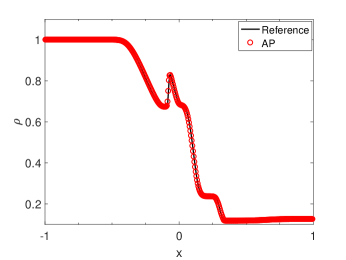
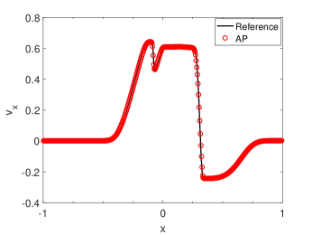
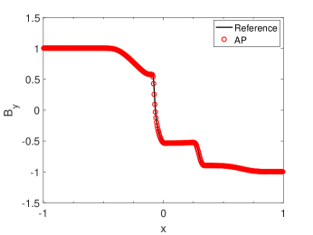
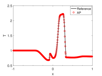
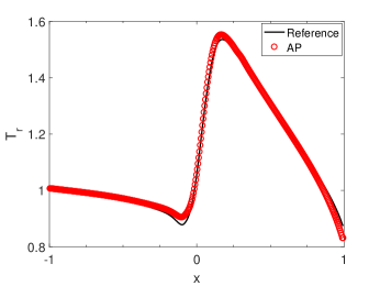
In the simulation of RMHD, it is a challenging task to produce accurate radiative shocks, especially in the optically thick regime. We test a range of the radiation-hydrodynamic shock problems presented in [lowrie2008radiative] in which several shocks are present in the solution. For each of these shocks, we set , adiabatic index for an ideal gas , absorption collision cross-section , scatter collision cross-section , , in RMHD system (2.2), and the radiation temperature . Moreover, the computational domain is and the results at are displayed. In this example, . In [lowrie2008radiative], the authors have obtained some semi-analytic solutions for the non-equilibrium diffusion limit system (2.3) at different Mach numbers. We compare the numerical results with the semi-analytic solutions obtained [lowrie2008radiative].
| (5.2) |
| (5.3) |
First of all, a Mach 1.2 shock is considered, which has no isothermal sonic point (ISP) but a hydrodynamic shock. The initial conditions are shown in (5.2). Fig. 3 compares our numerical results with the semi-analytic solutions, in which we can see good agreement for all quantities, including density, velocity, material and radiation temperature. Due to the hydrodynamic shock, there are discontinuities in the solution profiles of density, velocity and material temperature, and the maximum material temperature is bounded, since there is no ISP to drive it further.
At Mach 2, there are both a hydrodynamic shock and an ISP. The initial conditions are given in (5.3). Fig. 4 compares our numerical results with the semi-analytic solutions. One can see that our numerical results are in good agreement with the semi-analytic solutions. In Fig. 4, discontinuities can be seen in material density, velocity and material temperature due to the hydrodynamic shock. Moreover, the Zel’dovich spike can be observed in material temperature as in Fig. 4(c). The Zel’dovich spike is caused by the ISP embedded within the hydrodynamic shock, which drives up the material temperature at the shock front.
5.4. Example 4
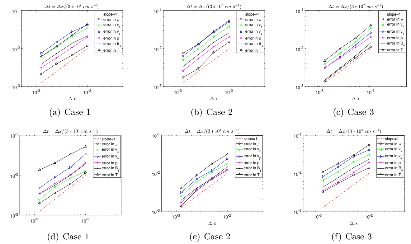
We show that the convergence order and stability of our scheme for the coupled RMHD system (1.1)-(1.2) are independent of the light speed. In this example we assume that the speed of light , the radiation constant . Three different sets of , are tested: 1) , ; 2) , ; 3) , . Moreover, the initial data for the three cases are the same as in Example 1 and the units of density, magnetic flux density and pressure are respectively , and . Since the exact solutions are not known, the numerical errors are defined by
| (5.4) | ||||
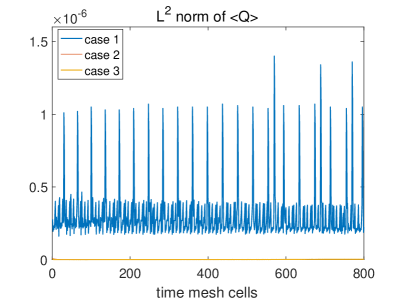
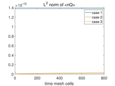
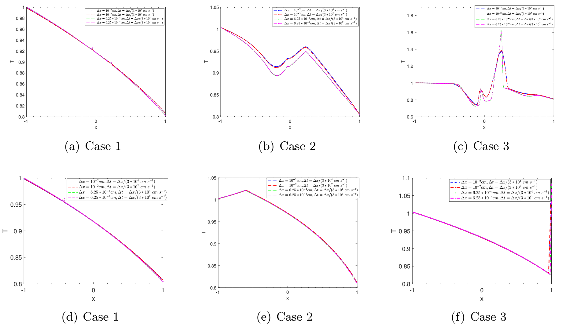
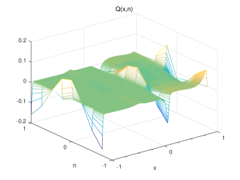
Different , , , , are tested and are chosen to be and . The convergence orders are displayed in Figure. 5 and we can see that the convergence orders are independent of the time step. And we plot the norm of and in each time step with and . We can see from Fig.6 that the values of and are close to zero. The two constraints and are not exactly satisfied due to numerical errors. However, we can consider of solving a new model system composed of , , and the MHD system, which can yields the solution to the original RMHD system. The results are acceptable except some numerical errors. Moreover, the CFL condition of explicit schemes requires that , but much larger time steps are allowed in our AP solver. To check the stability, we plot the numerical results of Case 1, 2 and 3 calculated by our AP solver with and two different , , and two different , . In Figure 7, we can observe that the stability does not depend on the time step but the accuracy does.
5.5. Example 5
The RMHD system with multi-scale absorption and scattering coefficients are tested in this example. The initial and boundary conditions are the same as in case 1 of Example 4. The absorption and scattering coefficients vary in space, such that
As we can see from the profile of in Fig. 8(a), varies from very small to very large, thus both optical thick and thin regimes coexist. To compute the reference solution, we use a finite volume solver in [sun2020multiscale] and a fine mesh , . We use , in our AP scheme, which is much larger than the allowed time step for the explicit solver. The numerical results at are displayed in Fig. 8(b)-(h). As we can see from Fig. 8(b) that is not small in some region, which indicate that one has to use RMHD system instead of the limit system. The good agreement between our solution and the reference solution indicates that our method works well for the coexisting case for the RMHD system.

6. Conclusion and discussions
In this paper, we have introduced an AP scheme in both space and time for the RMHD system that couples the ideal MHD equations with a gray RTE. Two different scalings are considered, one results in an equilibrium diffusion limit system, while the other results in nonequilibrium. The main idea is to decompose the intensity into three parts, two parts correspond to the zeroth and first order moments, while the third part is the residual. The two macroscopic moments are updated first by treating them implicitly while the residual explicitly. After the zeroth and first order moments are obtained, we update the residual term by solving implicitly a linear transport equation for each direction . For the space discretization, we use Roe’s method in the Athena code to solve the convective part in the ideal MHD equations and the UGKS for the RTE. Numerical results of optically thin and thick regions coexisting case are presented and the radiative shock problem are tested. The stability and convergence orders of the proposed scheme are independnent of the light speed. In each time step, our method requires nonlinear iterations to solve a system with only macroscopic quantities, which means the nonlinear iteration is independent of the number of angles. After the macroscopic quantities are obtained, decoupled linear transport equations are solved only once in each time step. The computational cost is much lower than a fully implicit solver. The scheme performance for real multi-dimensional anisotropic problem will be our future work.
It would be worthwhile to construct a second-order AP method for the radiation magnetohydrodynamics system. In the semi-implicit scheme, a simple time-integration method has been used. To obtain a second scheme, higher order IMEX time-integration method can be considered.
Acknowledgement: The authors would like to thank Dr. Yanfei Jiang from Computational Center for Astrophysics, the Flatiron Institute, for proposing this problem and useful discussions. S. Jin is partially supported by NSFC12031013 and the Strategic Priority Research Program of Chinese Academy of Sciences, XDA25010404; M. Tang and X. J. Zhang are partially supported by NSFC11871340 and the Strategic Priority Research Program of Chinese Academy of Sciences, XDA25010401.
Appendix A A The derivation of asymptotic analysis for the two regimes
In the non-equilibrium regime, the RMHD system (2.1) becomes:
| (A.1a) | |||||
| (A.1b) | |||||
| (A.1c) | |||||
| (A.1d) | |||||
| (A.1e) | |||||
where
When , we show that the solution to (2.2) can be approximated by the solution to a nonlinear diffusion equation coupled with a MHD system. We assume that the radiation intensity and temperature have the following Chapman-Enskog expansion such that
| (A.2) | |||
By substituting ansatz (A.2) into equation (2.2a) and collecting the terms of the same order in , we have
| (A.3a) | |||
| (A.3b) | |||
The term in equation (A.3b) equals to 0 due to equation (A.3a). Multiplying both sides of (2.2a) by , taking its integral with respect to and combining the obtained equation with (2.2c), one can get the following momentum conservation equation:
| (A.4) |
By using (A.3a) and (where denotes the 3 by 3 identity matrix), when , (A.4) gives
| (A.5) |
By taking the integral with respect to on both sides of (2.2a), and combining it with (2.2d), one can obtain the energy conservation equation
| (A.6) |
By using (A.3a), when , (A.6) gives
Noting (A.3b), we find
| (A.7) |
(2.2b), (A.5), (A.7) and (2.2e) give four equations for , to obtain a closed system, we need one more equation for . Taking on both sides of equation (2.2a), yields:
By using the expansion in (A.2) and (A.3a), the leading order terms are
then from (A.3b), one gets
| (A.8) |
Therefore, when in (2.2), the solution can be approximated by the solution of the following non-equilibrium system:
| (A.9a) | |||||
| (A.9b) | |||||
| (A.9c) | |||||
| (A.9d) | |||||
| (A.9e) | |||||
In the equilibrium regime, the RMHD system (2.1) becomes:
| (A.10a) | |||||
| (A.10b) | |||||
| (A.10c) | |||||
| (A.10d) | |||||
| (A.10e) | |||||
where
Using the same expansion as in (A.2), one has
| (A.11) | ||||
Then substituting (A.11) into (2.4a) and collecting the terms of the same order of , one gets
| (A.12a) | |||
| (A.12b) | |||
by similar calculations in section A, one can get the following equilibrium diffusion limit:
| (A.13a) | |||||
| (A.13b) | |||||
| (A.13c) | |||||
| (A.13d) | |||||
Appendix B B The processes of UGKS
Recall the RTE (4.1a) in the slab geometry. Integrating it over and gives
The microscopic flux is computed by solving the following initial value problem at the cell boundary :
| (B.1) |
In the UGKS scheme, we firstly assume the coefficients and in space and time are piecewise constant, thus the radiative transfer equation in RMHD system (4.1) is equivalent to
| (B.2) |
with . Solving the equivalent equation (B.2) with the initial value in the system (B.1), which gives the solution
| (B.3) | ||||
with , and being the constant value at the corresponding cell boundary for , and respectively. In solution (B.3), there remains three terms that need to approximate: the first one is the initial condition around , namely the function ; the second one is the two functions localized in the time interval and around the boundary , i.e., the functions and ; the last one is the term .
The first term:
For the first term, a piecewise constant reconstruction function is used to approximate the initial function around :
| (B.4) |
The second term:
For the second term, the approximations of two functions and between and and around are constructed in the same manner, so only the approximation of is introduced in detail. The function is treated implicitly in time by using piecewise linear polynomials, so the reconstruction for reads:
| (B.5) |
with the interface value of defined by
and with the spatial derivatives given by
The third term:
At last, the approximation for the term is discussed. Recall the definition of :
The upwind scheme is used to determine , i.e., the value of at the center of the interval is determined by the velocity field at the both sides boundary,
| (B.6) |