Validity of compressibility equation and Kirkwood-Buff theory in crystalline matter

Abstract

Volume integrals over the radial pair-distribution function, so-called Kirkwood-Buff integrals (KBI) play a central role in the theory of solutions, by linking structural with thermodynamic information. The simplest example is the compressibility equation, a fundamental relation in statistical mechanics of fluids. Until now, KBI theory could not be applied to crystals, because the integrals strongly diverge when computed in the standard way. We solve the divergence problem and generalize KBI theory to crystalline matter by using the recently proposed finite-volume theory. For crystals with harmonic interaction, we derive an analytic expression for the peak shape of the pair-distribution function at finite temperature. From this we demonstrate that the compressibility equation holds exactly in harmonic crystals.

In statistical mechanics a close link exists between fluctuations of extensive variables and response functions. For example, the density and concentration fluctuations in a fluid are directly related to the isothermal compressibility, partial molar volumes and diffusion coefficients mcquarrie ; bennaim ; guevara20 . Density fluctuations can be accessed experimentally as the long-wave-length limit of the structure factor and theoretically from volume integrals over the pair-distribution function (PDF), so-called Kirkwood-Buff integrals (KBIs) kb52 . KBI theory was developed for fluids, i.e. homogeneous and isotropic systems. In solids, these symmetries are sponspontaneously broken and statistical mechanics commonly starts from the perfect crystal landau . Defects and lattice vibrations are treated as a perturbation ashcroft . This approach is efficient at low temperature and low defect concentration, but it breaks down near the solid-liquid phase transition and in amorphous and nanostructured materials. Therefore a common set of statistical mechanical techniques, valid for all states of matter is highly desirable. The PDF should be a key element of such a framework, since it can be easily obtained for all kinds of matter billinge07 , including amorphous and crystalline solids toby ; proffen05 , liquids and gases. This raises the question whether KBI theory, which is a cornerstone of the theory of solutions bennaim ; kb52 ; shulgin06 ; milzetti18 , is valid in the solid state. Surprisingly, this basic question has, to the best of our knowledge, not yet been answered.

In this letter, we demonstrate that KBI theory is valid for crystalline matter, i.e. thermodynamic quantities such as the isothermal compressibility, can be obtained from the PDF, in principle in the same way as in fluids. In crystals, KBIs diverge when computed in the standard way as “running” integrals. We solve the divergence problem by starting from the recently developed KBI theory for finite volumes kruger13 . For a monoatomic crystal with harmonic interactions, we derive an analytic expression for the thermal broadening of the PDF. From this we calculate the crystal KBI at finite temperatures and demonstrate that the compressibility equation holds exactly in harmonic crystals. Our findings extend the validity and applicability of KBI theory, hitherto used only in homogeneous fluids, to all phases of matter, and thus open up new ways for the thermodynamic modeling of complex materials.

We consider a monoatomic system for simplicity. Generalization of the present theory to multicomponent systems is straightforward. The instantaneous position of particle $i$ is ${\bf r}_{i}$. The single-particle density is given by $\rho({\bf r})=\langle\sum_{i}\delta({\bf r}-{\bf r}_{i})\rangle$, where $\langle\dots\rangle$ denotes the grand-canonical ensemble average. The PDF is defined as

$$g({\bf r}^{\prime},{\bf r}^{\prime\prime})=\frac{\langle\sum_{i\neq j}\delta({\bf r}^{\prime}-{\bf r}_{i})\delta({\bf r}^{\prime\prime}-{\bf r}_{j})\rangle}{\rho({\bf r}^{\prime})\rho({\bf r}^{\prime\prime})}\;.$$ (1)

For a homogeneous and isotropic system the density is constant $\rho({\bf r})=\rho$. The PDF depends only on the pair distance $r=|{\bf r}|=|{\bf r}^{\prime}-{\bf r}^{\prime\prime}|$ and simplifies to

$$g(r)=\frac{1}{V\rho^{2}}\langle\sum_{i\neq j}\delta({\bf r}-{\bf r}_{i}+{\bf r}_{j})\rangle\;,$$ (2)

where $V$ is the volume of the system. In a crystal, the translational and rotational symmetry are broken, and so Eq. (2) does not follow directly from Eq. (1). Here we consider the statistical ensemble of arbitrarily shifted and rotated crystals, corresponding to a powder sample kruger20 . Since this ensemble is homogeneous and isotropic, Eq. (2) is valid and commonly used in powder diffraction analysis toby . The finite-volume KBI is defined as kruger13

$$G^{V}=\frac{1}{V}\int_{V}d{\bf r}^{\prime}\int_{V}d{\bf r}^{\prime\prime}(g(r)-1)\;.$$ (3)

By inserting Eq. (2) into (3) we obtain the well-known relation between the KBI and the particle number fluctuations in the volume $V$ kb52 ; kruger13

$$\Gamma^{-1}(V)\equiv\frac{\langle N^{2}\rangle-\langle N\rangle^{2}}{\langle N\rangle}=1+\rho G^{V}\;,$$ (4)

where $N$ is the instantaneous number of particles in $V$ and $\langle N\rangle=\rho V$ is its grand-canonical ensemble average. We shall refer to $\Gamma^{-1}$ as the fluctuation function. It is also known as the thermodynamic correction factor schnell11 .

We first consider a perfect crystal at zero temperature neglecting zero-point motion. The PDF in Eq. (2) becomes

$$4\pi r^{2}\rho\;g(r)=\sum_{{\bf R}\neq{\bf 0}}\delta(r-|{\bf R}|)=\sum_{s=1}^{\infty}n_{s}\delta(r-R_{s})\;,$$ (5)

where ${\bf R}$ are the lattice sites and the sum on the r.h.s. runs over shells $s$, containing $n_{s}$ lattice points at a distance $R_{s}$ from the origin. Throughout this paper, the nearest neighbor distance $d$ is taken as the unit length. The PDF of the fcc lattice is shown in Fig. 1 a. It compares well with low temperature PDF data of fcc crystals, such as Al toby . In the limit $V\rightarrow\infty$, Eq. (3) simplifies to kb52

$$G^{\infty}=\int_{0}^{\infty}(g(r)-1)4\pi r^{2}dr\;,$$ (6)

provided that the integrals in Eq. (3) converge absolutely. This condition is met in fluids, since $g(r)-1$ vanishes for distances larger than the correlation length. KBIs are commonly computed as running integrals,

$$G_{0}(L)=\int_{0}^{L}(g(r)-1)4\pi r^{2}dr\;,$$ (7)

where $L$ is a cut-off radius. The corresponding fluctuation function $\Gamma^{-1}_{0}(L)=1+\rho G_{0}(L)$, is plotted in Fig. 1 b. It shows large oscillations whose amplitude grows linearly with $L$. Comparing Figs 1 a and 1 b, we see that the oscillations of the PDF become strongly amplified upon volume integration. This effect may also occur in liquids for small $L$ kruger13 . However, in liquids the running KBI eventually converges, namely when $L$ exceeds the correlation length. In a crystal, the correlation length is infinite and the running KBI never converges. From this result, one might think that KBI theory cannot be applied to crystals. We now show that this is not true and we devise a method for calculating KBIs in crystals.

The finite volume KBI in Eq. (3) can be transformed exactly to a one-dimensional integral kruger13 ; dawass18 as

$$G^{V}=G(L)=\int_{0}^{L}(g(r)-1)y(r/L)4\pi r^{2}dr\;,$$ (8)

where $y(x)$ is a geometrical function characteristic of the shape of the volume $V$ and $L$ is the maximum distance between any two points in $V$. We consider a sphere of diameter $L$. In this case, $y(x)=1-3x/2+x^{3}/2$, $x=r/L$ kruger13 .

The fluctuation function $\Gamma^{-1}(L)$ obtained with the finite-volume KBI of Eq. (8) is shown in Fig. 1 c. It clearly converges for $L\rightarrow\infty$, in sharp contrast to the running KBI (Fig. 1 b). We find $\Gamma^{-1}(L)\rightarrow 0$, which is the correct limit, since the particles are immobile in a perfect crystal and thus the particle number fluctuations must vanish for $V\rightarrow\infty$. For a system with finite correlation length, e.g. a fluid away from the critical point, we previously proved that $\Gamma^{-1}(L)-\Gamma^{-1}(\infty)$ varies as $1/L$ kruger13 . As seen in Fig. 1 c, this also holds for crystals, despite the fact that the particle positions are correlated over infinite distances. Importantly, $\Gamma^{-1}(L)$ is strictly positive, which is a necessary property of a variance (Eq. 4). In contrast, $\Gamma_{0}^{-1}(L)$ (Fig. 1 b) is not always positive, and thus does not describe particle fluctuations for finite $L$ dawass18 ; kruger18 .

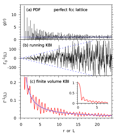
Figure 1: PDF $g(r)$ and correlation function $\Gamma^{-1}(L)$, Eq. (4), of a perfect fcc lattice. $r$ is the pair distance and $L$ is the upper integration bound. The nearest neighbor distance $d$ is taken as unit length. (a) PDF as histogram plot with bin size $\Delta r=0.05$. (b) $\Gamma^{-1}_{0}(L)$ computed with running KBI, Eq. (7). (c) $\Gamma^{-1}(L)$ computed with finite-volume KBI, Eq. (8). The inset shows $\Gamma^{-1}(L)$ on the full $y$-scale. The blue lines are a guide to the eye. They are $y=1$ in (a), $y=\pm 10L$ in (b), $y=0.33/L$ in (c).

At finite temperature, the peaks of the PDF become broadened due to vibrations of the atoms around their equilibrium positions. We now derive an analytic expression for the broadening function of a monoatomic harmonic crystal. Let ${\bf R}+{\bf u}$ be the instantaneous position of the atom at lattice site ${\bf R}$ and ${\bf u}$ the displacement vector. A lattice vibration is described by

$${\bf u}_{\bf k}({\bf R},t)={\bf u}_{{\bf k},0}\cos({\bf k}\cdot{\bf R}-\omega_{\bf k}t)\;,$$ (9)

where ${\bf k}$ is the wave vector, ${\omega_{\bf k}}$ the frequency and ${\bf u}_{{\bf k},0}$ the amplitude. For each ${\bf k}$ there are three modes with different polarization $\lambda$. We first consider any one of them. The amplitude ${\bf u}_{{\bf k},0}$ is related to the temperature through the equipartition theorem as

$$\frac{1}{2}k_{B}T=\frac{1}{2}m\omega_{\bf k}^{2}\sum_{\bf R}\langle{u}_{\bf k}({\bf R},t)^{2}\rangle=\frac{1}{4}Nm\omega_{\bf k}^{2}{u}_{{\bf k},0}^{2}\;,$$ (10)

where $\langle\dots\rangle$ denotes the time average and $N$ is the number of atoms. The relative displacement of the atom at site ${\bf R}$ with respect to the atom at site ${\bf 0}$ is $\Delta{\bf u}_{{\bf k}}({\bf R},t)={\bf u}_{{\bf k}}({\bf R},t)-{\bf u}_{{\bf k}}({\bf 0},t)$. From Eq. (9), the time average of the square of the relative displacement is easily found to be

$$\langle\Delta{u}_{\bf k}({\bf R})^{2}\rangle={u}_{{\bf k},0}^{2}(1-\cos{\bf k}\cdot{\bf R})\;.$$ (11)

In the harmonic approximation the phonons are independent and so the mean square displacement is additive. Therefore the total mean square $\sigma^{2}\equiv\langle\Delta{u}({\bf R})^{2}\rangle$ is obtained by summing (11) over all wave vectors in the Brillouin zone. This yields

$$\sigma^{2}=\frac{2k_{B}T}{mN}\frac{V}{8\pi^{2}}\int_{BZ}d{\bf k}\frac{1-\cos{\bf k}\cdot{\bf R}}{\omega_{\bf k}^{2}}\;,$$ (12)

where $V$ is the volume of the crystal. Here, the $k$-space volume element $d{\bf k}=8\pi^{3}/V$ and Eq. (10) have been used. We now make the Debye approximation, i.e. we assume $\omega_{\bf k}=ck$, where $c$ is the speed of sound and we replace the Brillouin zone by a sphere of radius $k_{D}=(6\pi^{2}\rho)^{1/3}$ where $\rho=N/V$ is the atomic density. After a straightforward integration over the angular coordinates of ${\bf k}$, we obtain

$$\sigma^{2}=\frac{k_{B}T}{\rho mc^{2}}\frac{1}{\pi^{2}}\left(k_{D}-\frac{1}{R}\int_{0}^{x_{D}}\frac{\sin x}{x}dx\right)\;,$$ (13)

where $x_{D}\equiv k_{D}R$. We write $\rho=(\gamma/d)^{3}$, where $d$ is the nearest neighbor distance and $\gamma$ is a dimensionless factor which depends on the lattice type. $\gamma=1$ for simple cubic and $\gamma=2^{1/6}\approx 1.12$ for close-packed lattices. We have $x_{D}=\gamma(6\pi^{2})^{1/3}R/d\approx 4R/d$. As we are interested in the regime $R\gg d$, we can safely take the limit $x_{D}\rightarrow\infty$ in the integral in Eq. (13). The integral then becomes $\pi/2$ and we obtain

$$\sigma^{2}=\frac{k_{B}T}{mc^{2}}\;d^{2}\left(\alpha-\beta\frac{d}{R}\right)\;,$$ (14)

where $\alpha=(6/\pi)^{1/3}/(\pi\gamma^{2})$ and $\beta=1/(2\pi\gamma^{3})$. For a close-packed lattice we have $\alpha=0.31345$, $\beta=0.11254$. Eq. (14) is the variance of the probability distribution of the relative displacement $\Delta{\bf u}$ of an atom at a distance $R$ with respect to the atom at the origin, for one phonon polarization $\lambda$. Being the sum of many independent modes, the probability distribution can be taken as Gaussian. Upon summing over the three polarizations $\lambda$, the distribution is also isotropic. We consider the distance vector ${\bf r}$ between the atom at site ${\bf R}$ and the atom at site ${\bf 0}$. It is given by ${\bf r}={\bf R}+\Delta{\bf u}({\bf R)}$. Its probability distribution is a three-dimensional Gaussian centered at ${\bf R}$,

$$P({\bf r},{\bf R})=\frac{1}{(\sqrt{2\pi}\sigma)^{3}}\exp\left(-\frac{({\bf r}-{\bf R})^{2}}{2\sigma^{2}}\right)\;.$$ (15)

For the PDF we need the corresponding radial distribution, obtained by multiplying Eq. (15) by $r^{2}$ and integrating over the angles of ${\bf r}$. We use spherical coordinates with the $z$-axis along ${\bf R}$. After some straightforward algebra, we find the radial probability distribution function

$$P(r,R)=\frac{1}{\sqrt{2\pi}\;\sigma}\frac{r}{R}\times$$

$$\left(\exp\left({-\frac{(r-R)^{2}}{2\sigma^{2}}}\right)-\exp\left({-\frac{(r+R)^{2}}{2\sigma^{2}}}\right)\right)\;,$$ (16)

where $\sigma$ is a function of $R$, given by Eq. (14). The PDF of the harmonic crystal at finite temperature is obtained by replacing the delta-functions in the zero-temperature PDF, Eq.(5), by the peak function (16), which yields

$$4\pi r^{2}\rho\;g(r)=\sum_{s=1}^{\infty}n_{s}P(r,R_{s})\;.$$ (17)

The temperature dependence comes from the peak width $\sigma(R,T)$ given by Eq. (14). In the following we shall refer to the reduced temperature $T/T_{0}$, where $T_{0}\equiv mc^{2}/k_{B}$. Note that in the harmonic approximation the speed of sound $c$ is temperature independent and so $T_{0}$ is a constant.

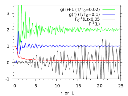
Figure 2: PDF $g(r)$ and fluctuation function $\Gamma^{-1}(L)$ at finite temperature for the fcc crystal in the harmonic approximation. The top-most (green) curve is the PDF for $T/T_{0}=0.02$, shifted up by 1 for clarity. All other curves are obtained with $T/T_{0}=0.1$. $\Gamma^{-1}$ (red) and $\Gamma_{0}^{-1}$ (black) correspond to running and finite volume KBI, respectively. Note that $\Gamma_{0}^{-1}$ is multiplied by a factor of 0.05.

In Fig. 2 the PDF $g(r)$ of Eq. (17) is plotted for $T/T_{0}=0.02$ (green line) and $T/T_{0}=0.1$ (blue line) for the fcc crystal. As expected, the PDF becomes smoother with increasing temperature, but its oscillations do not decay exponentially. From the PDF for $T/T_{0}=0.1$, the fluctuation function is computed with either running or finite volume KBI. The running KBI $\Gamma_{0}^{-1}(L)$ (black line) strongly diverges. Comparison with the $T=0$ result in Fig. 1 shows that the oscillations are reduced at finite temperature but they still increase linearly with $L$. As a consequence, the running KBI cannot be used for crystals, even at finite temperature. In contrast, the result obtained with the finite-volume KBI ($\Gamma^{-1}(L)$, red line) converges smoothly to a finite, positive limit $\Gamma^{-1}(\infty)$.

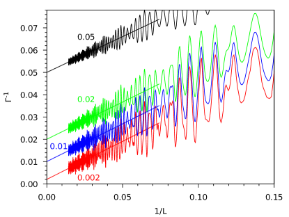
Figure 3: $L\rightarrow\infty$ convergence of the fluctuation function $\Gamma^{-1}(L)$ of the harmonic fcc crystal obtained with finite-volume KBI. The reduced temperature $T/T_{0}$ is indicated on each curve. The straight lines are linear fits in the range $1/L<0.075$.

In Fig. 3 the convergence of $\Gamma^{-1}(L)$ is studied as a function of $1/L$ for reduced temperatures $T/T_{0}$ in the range from 0.002 to 0.05. Assuming $T_{0}=5000$ K, which is a typical value for solid argon, this corresponds to $T$=10–250 K. It can be seen that at all temperatures, the oscillations are large, but the curves clearly converge to $\Gamma^{-1}(\infty)=T/T_{0}$. This is the value predicted by the compressibility equation as will be shown below. The numerical values of $\Gamma^{-1}(\infty)$, obtained from a linear regression of the curves in the range $1/L<0.075$ (straight lines in Fig. 3) are 0.05003, 0.02005, 0.01005, 0.00206. With respect to the theoretical value $T/T_{0}$ the absolute error is about $5\times 10^{-5}$ in all cases and the relative error varies between 0.06% and 3%. It is interesting to note that the correct temperature dependence of the KBI depends crucially on using the exact form of the peak shape, Eq. (16) and peak width, Eq. (14). In Fig. 4 the fluctuation function $\Gamma^{-1}(L)$ is computed for slightly modified peak shapes.

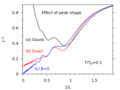
Figure 4: Effect of peak shape on fluctuation function $\Gamma^{-1}(L)$ of an fcc crystal at $T/T_{0}=0.1$, obtained with finite-volume KBI. (a) Simple Gaussian shape. (b) Exact shape and width (Eqs 14,16). (c) Exact shape, but constant width ($\beta=0$ in Eq. 14).

First, if the peak function (16) is replaced by a simple, normalized Gaussian of the same width, then $\Gamma^{-1}$ diverges (Fig. 4 (a), black line). Second, if the exact peak shape Eq. (16) is used but with a fixed peak width, i.e. $\beta=0$ in Eq. (14), then $\Gamma^{-1}(L)$ converges to zero instead of $T/T_{0}$ for $L\rightarrow\infty$ (Fig. 4 (c), blue line). At finite temperature, $\Gamma^{-1}(\infty)=0$ implies vanishing compressibility, which is unphysical. Comparison between Fig. 4 (b) and (c) also shows that the temperature dependence of the KBI is entirely due to the small variation of the PDF peak width with distance, i.e. the $1/R$ term in Eq. (14).

From the results in Fig. 3 we conclude that the finite-volume KBI of the harmonic crystal converges to $\Gamma^{-1}(\infty)=T/T_{0}$ for any temperature, where $T_{0}=mc^{2}/k_{B}$ by definition. The speed of sound $c$ is related to the isentropic compressibility $\kappa_{S}$, by the Newton-Laplace equation, $\kappa_{S}=(\rho mc^{2})^{-1}$, which holds in any phase of matter. Thus we have $\Gamma^{-1}(\infty)=\kappa_{S}\rho k_{B}T$. In condensed matter, $\kappa_{S}\approx\kappa_{T}$ where $\kappa_{T}$ is the isothermal compressibility. Equality holds exactly when the thermal expansion is zero, which is the case for harmonic interaction considered here ashcroft . With Eq. (4), it follows that $1+\rho G^{\infty}\equiv\Gamma^{-1}(\infty)=\kappa_{T}\rho k_{B}T$. This is the compressibility equation mcquarrie ; bennaim ; landau . We have thus proved that this fundamental relation of the statistical mechanics of fluids, also holds in crystalline solids. The only difference between fluids and solids is the way how $G^{\infty}$ can be computed. In fluids, the finite-volume KBI $G^{V}$ in Eq. (3) converges absolutely and so the infinite volume limit $G^{\infty}$ can be obtained with the usual expression, Eq. (6). In crystals, where the correlation length is infinite, $G^{V}$ does not converge absolutely and so the order of integration in Eq. (3) cannot be changed at will. As a consequence, the standard expression of $G^{\infty}$, Eq. (6) is ill-defined and the running KBI (7) cannot be used. Instead, $G^{\infty}$ must be calculated with the finite-volume KBI, $G^{V}$ (Eq. 3) or $G(L)$ (Eq. 8). Our findings show that KBI theory can be applied to crystals, and that the compressibility can be obtained form the PDF in the same way as in liquids, provided that the finite-volume KBI method kruger13 is employed. Here we have used the harmonic approximation and have disregarded quantum zero-point motion, in order to obtain analytical results. Anharmonic effects play an important role in the thermodynamic of solids, and must be taken into account for comparison with experiment. Anharmonic and quantum effects will modify the PDF, which may be computed using molecular simulations miyaji21 . However, this does not change the way how the KBI is obtained from the PDF.

In summary, we have generalized KBI theory, which is widely used in fluids, to crystalline solids. The divergence of standard KBI has been solved by using the finite volume KBI theory. For a harmonic crystal, we have derived an analytic expression for the PDF peak shape and have proved that the compressibility equation holds exactly. The present findings show that KBI is fully valid in solids, and thus opens new avenues for the thermodynamic modeling of structurally complex matter and for solid-liquid phase transitions.

- (1) D. A. McQuarrie, Statistical Mechanics, Harper&Row, New York, 1973.
- (2) A. Ben-Naim, Molecular Theory of Solutions, Oxford Univ. Press (2006).
- (3) G. Guevara-Carrion, R. Fingerhut, and J. Vrabec, Fick Diffusion Coefficient Matrix of a Quaternary Liquid Mixture by Molecular Dynamics, J. Phys. Chem. B 124, 4527 (2020).
- (4) J. G. Kirkwood, and F. P. Buff, The statistical mechanical theory of solutions. I, J. Chem. Phys. 19, 774 (1951).
- (5) L. D. Landau, E. M. Lifshitz, Statistical Physics, Part 1, 3rd ed., Butterworth-Heinemann, Oxford, 1980.
- (6) N. W. Ashcroft and N. D. Mermin, Solid State Physics, Holt, Rinehart and Winston, New York, 1976, Chapter 25.
- (7) S. J. L. Billinge and I. Levin, The Problem with Determining Atomic Structure at the Nanoscale, Science 316, 561-565 (2007).
- (8) B. H. Toby, T. Enami, Accuracy of Pair Distribution Function Analysis Applied to Crystalline and Non-Crystalline Materials, Acta Cryst. A 48, 336 (1992).
- (9) T. Proffen, K. L. Page. S. E. McLain, B. Clausen, T. W. Darling, J. A. TenCate, S.-Y. Lee, E. Ustundag, Atomic pair distributition function analysis of materials containing crystalline and amorphous phases, Z. Kristallogr. 220, 1002-1008 (2005).
- (10) I. L. Shulgin and E. Ruckenstein, The Kirkwood-Buff Theory of Solutions and the Local Composition of Liquid Mixtures, J. Phys. Chem. B 110, 12707 (2006).
- (11) J. Milzetti, D. Nayar, N. F. A. van der Vegt, Convergence of Kirkwood-Buff Integrals of Ideal and Nonideal Aqueous Solutions Using Molecular Dynamics Simulations, J. Phys. Chem. B 122, 5515 (2018).
- (12) P. Krüger, S. K. Schnell, D. Bedeaux, S. Kjelstrup, T. J. H. Vlugt and J.-M. Simon, Kirkwood-Buff integrals for finite volumes J. Phys. Chem. Lett. 4, 235 (2013).
- (13) P. Krüger, Ensemble averaged Madelung energies of finite volumes and surfaces, Phys. Rev. B 101, 205423 (2020).
- (14) S. K. Schnell, X. Liu, J.-M. Simon, A. Bardow, D. Bedeaux, T. J. H. Vlugt, S. Kjelstrup, Calculating thermodynamic properties from fluctuations at small scales, J. Phys. Chem. B 115, 10911 (2011).
- (15) N. Dawass, P. Krüger, S. K. Schnell, D. Bedeaux, S. Kjelstrup, J.-M. Simon and T. J. H. Vlugt, Finite-size effects of Kirkwood-Buff integrals from molecular simulations, Mol. Sim. 44, 599 (2018).
- (16) P. Krüger and T. J. H. Vlugt, Size and shape dependence of finite-volume Kirkwood-Buff integrals, Phys. Rev. E 97, 051301(R) (2018).
- (17) M. Miyaji, B. Radola, J.-M. Simon and P. Krüger, Extension of Kirkwood-Buff theory to solids and its application to the compressibility of fcc argon, J. Chem. Phys. 154, 164506 (2021).