Transformations of Rectangular Dualizable Graphs

Abstract

A plane graph is said to be a rectangular graph if each of its edges can be oriented horizontal or vertical, its internal regions are four-sided and it has a rectangular enclosure. If dual of a planar graph is a rectangular graph, then the graph is said to be a rectangular dualizable graph (RDG). In this paper, we present adjacency transformations between RDGs and present polynomial time algorithms for their transformations.

An RDG $\mathcal{G}=(V,E)$ is called maximal RDG (MRDG) if there does not exist an RDG $\mathcal{G^{\prime}}=(V,E^{\prime})$ with $E^{\prime}\supset E$. An RDG $\mathcal{G}=(V,E)$ is said to be an edge-reducible if there exists an RDG $\mathcal{G^{\prime}}=(V,E^{\prime})$ such that $E\supset E^{\prime}$. If an RDG is not edge-reducible, it is said to be an edge-irreducible RDG. We show that there always exists an MRDG for a given RDG. We also show that an MRDG is edge-reducible and can always be transformed to a minimal one (an edge-irreducible RDG).

1 Introduction

Due to advances in VLSI technology, interconnection optimization is of the major concern [1], i.e., it is sometimes required to improve the interconnections of an existing VLSI circuit. The modification of interconnection can be seen in two ways: interconnection among modules and interconnection of modules to the outside units. To deal with the first case, we need to increase/decrease the adjacency relations among the modules as much as possible and the second requires to increase the length (the number of modules adjacent to the exterior) of exterior of the layout. Architecturally, a legacy rectangular floorplan (RFP) can be reconstructed to suit modern lifestyles by changing the adjacency relations of its rooms/rectangles. In this paper, we address the graph theoretic characterization to deal with the issues of interconnections in floorplanning.

For a better understanding of the further text, we first explain the geometric duality relation between planar graphs and rectangular floorplans (RFPs). A graph $\mathcal{H}$ is called dual graph of a plane graph $\mathcal{G}$ if there is one to one corresponding between the vertices of $\mathcal{G}$ and the regions of $\mathcal{H}$ and whenever any two vertices of $\mathcal{G}$ are adjacent, the corresponding regions of $\mathcal{H}$ are adjacent. A plane graph $\mathcal{G}$ is called rectangular graph if each of its edges can be oriented horizontal or vertical, its internal regions are four-sided and it has a rectangular enclosure. A graph admitting a rectangular dual graph is said to be a rectangular dualizable graph (RDG). A rectangular floorplan (RFP) can be seen as a particular embedding of the dual of an RDG and is defined as a partition of a rectangle $\mathcal{R}$ into $n$-rectangles $R_{1},R_{2},\dots,R_{n}$ such that no four of them meet at a point. Fig. 1 demonstrates the rectangular dualization method, i.e., the geometric duality relationship of planar graphs and rectangular floor-plans. Consider the graph in Fig. 1a, whose extended graph is shown in Fig 1b. It is dualized in Fig. 1c where a region $R_{i}$ corresponds to a vertex $v_{i}$. Further, on orienting each side of all regions of the dualized graph, horizontally or vertically, we obtain an RFP as shown in Fig 1d.

The point where three or more rectangles of a given RFP meet is called a joint. We know that an RFP has 3-joints and 4-joints only where 4-joints are regarded as a limiting case of 3-joints [2]. Hence, abiding by the common design practices, we restrict ourselves to 3-joints only. Therefore throughout the paper, we transform an RFP with 3-joints to another RFP with 3-joints. The dual graph of such an RFP is always plane triangulated graph.

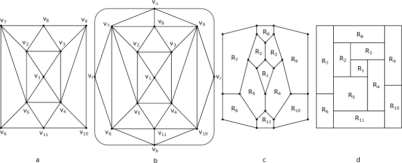
Figure 1: Rectangular dualization: (a) plane graph, (b) extended plane graph, (c) rectangular dual graph and (d) rectangular floorplan

1.1 Related work

The theory of RDGs is very restrictive [3, 4, 5]. Constructive RFP algorithms [6, 7, 8, 9] based on this theory emphasizes on the packing of rectangles into a rectangular area. Due to recent developments in the technology (VLSI design and architectural floorplanning), sometimes it is required to transform an existing RFP to another RFP, if possible. Here, the idea is to recursively improve an existing RFP until an optimal solution based on the user requirements, is attained.

From graph theoretic context, RFP transformation techniques have not been much emphasized. It has been addressed by authors [10, 11, 12] where a topologically distinct RFP was obtained from an existing one for a given graph while preserving the adjacency relations of the existing one. Wang et al. [13] modified an existing RFP by inserting or removing a rectangle to it. Contrary to this, in this paper, we address RFP transformation technique from a graph theoretic context which is based on changing adjacency relations among rectangles. For any two given adjacent rectangles of an RFP, it is interesting to identify whether they can be made nonadjacent in such a way that adjacency relations of remaining rectangles of the RFP remains sustained and the resultant floor-plan is an RFP. Conversely, can any two given non-adjacent rectangles of an RFP be made adjacent in such a way that adjacency relations of the remaining rectangles of the RFP remains preserved and the resultant floor-plan is an RFP?

Enumerating of all RFPs composed of $n$-rectangles has been remained a major issue in combinatorics [14, 15, 16, 17, 18, 19]. These methods are not preferable because they produce large solution space and therefore, it is computationally hard to pick an RFP suiting adjacency requirements of rectangles from such a large solution space.

In this paper, we present transformations between RFPs from graph theoretic context. However with the renewed interest in floorplannings, orthogonal floorplans from the graph theoretic context has also been well studied [20, 21, 22, 23, 24].

1.2 Our Results

Our main contribution is in two folds: (1). For a given RDG, we aim to construct a new RDG by introducing new adjacency relations while preserving all the existing adjacency relations until no more adjacency relation can be added. (2). For a given RDG, we aim to construct a new RDG by deleting adjacency relations while preserving all the other adjacency relations until no more adjacency relation can be removed. We first prove that these transformations are always possible and then present quadratic time algorithms for them.

The class of maximal RDGs (MRDGs) can play an important role in floorplanning because they are rich in adjacency relations. Therefore, it is interesting to construct an MRDG of a given RDG. Intuitively speaking, an MRDG is an RDG having maximal adjacency relations among its vertices. In fact, an MRDG with $n$ vertices has $2n-2$ or $3n-7$ edges. We show that there always exists an MRDG for a given RDG. Then we present a polynomial time algorithm that constructs the MRDG for the given RDG by adding new edges among its nonadjacent vertices. The number of such new edges is $2n-2-k$ or $3n-7-k$ where $k$ is the number of edges in the RDG. It would be more interesting if the given RDG is a path graph because then it requires the new edges to be added in bulk. Equivalently the new edges in bulk can be added to a Hamiltonian path of the given RDG to realize a new desired form of the RDG. We also show that a given MRDG is always edge-reducible and can be reduced to an RDG and present an algorithm that deletes the edges of a given RDG in until it is an RDG.

In this way, we can just add or remove those edges of the RDG that are missing from one of the RDG and we are done.

A brief description of the rest of the paper is as follows. In this article, we first survey the existing facts about RDGs in Section 2. In Section 3, we introduce MRDGs and edge-reducible RDGs. Then we show that an MRDG has $2n-2$ or $3n-7$ edges. MRDGs with $2n-2$ edges are wheel graphs whereas MRDGs with $3n-7$ edges are obtained from the class of maximal plane graphs with the property that they do not have any separating triangles in their interiors by deleting one of their exterior edges. In Section 4, we prove that it is always possible to construct an MRDG for a given RDG and present an algorithm for its construction from the given RDG. In Section 5, we show that it is always possible to transform an edge-reducible RDG to another RDG and present an algorithm for its reduction to a minimal one. Finally, we conclude our contributions and discuss future task in Section 6.

A list of notations used in this paper can be seen in Table 1.

Symbol	Description
RFP	rectangular floorplan
RDG	rectangular dualizable graph
MRDG	maximal rectangular dualizable graph
$v_{i}$	$i^{\text{th}}$ vertex of a graph
$d(v_{i})$	degree of $v_{i}$
$(v_{i},v_{j})$	an edge incident to vertices $v_{i}$ and $v_{j}$
3-cycle	a cycle of length 3
$v_{i}v_{j}v_{k}$	a cycle passing through vertices $v_{i}$, $v_{j}$ and $v_{k}$ of an RDG
$R_{i}$	a rectangle corresponding $v_{i}$
$E_{i}$	edge set of graph $\mathcal{G}_{i}$
$|E|$	cardinality of a set $E$
CIP(s)	corner implying path(s)

Table 1: List of Notations

2 Preliminaries

In this section, we survey some existing facts about RDGs which would be helpful in the coming sections.

A planar graph is a graph that can be embedded in the plane without crossings. A plane graph is a planar graph with a fixed planar embedding. It partitions the plane into connected regions called faces; the unbounded region is the exterior face (the outermost face) and all other faces are interior faces. The vertices lying on the exterior face are exterior vertices and all other vertices are interior vertices. A planar (plane) graph is maximal if no new edge can be added to it without disturbing planarity. Thus each face of a maximal plane graph is a triangle (including exterior face). If a connected graph has a cut vertex, then it is called a separable graph, otherwise it is called a nonseparable graph. Since floor-plans are concerned with connectivity, we only consider nonseparable (biconnected) and separable connected graphs in this paper.

Definition 2.1.

A graph is said to be rectangular graph if each of its edges can be oriented horizontally or vertically such that it encloses a rectangular area. If the dual graph of a planar graph is a rectangular graph, then the graph is said to be a rectangular dualizable graph (RDG). In other words, a planar graph is rectangular dualizable (RDG) if its dual can be realized as a rectangular floorplan (RFP). An RFP is a partition of a rectangle $\mathcal{R}$ into $n$ rectangles $R_{1},R_{2},\dots,R_{n}$ provided that no four of them meet at a point.

Theorems 2.1 and 2.2 talks about the existence of an RDG, where the following definitions are required.

Definition 2.2.

[6] A separating triangle is a cycle of length 3 in a plane graph that encloses atleast one vertex inside as well as outside. It is also known as a complex triangle.

Consider the graph shown in Fig. 2b having a cycle $\mathcal{C}$ of length 3 passing through the vertices $v_{1}$, $v_{2}$ and $v_{9}$, enclosing the vertices $v_{4}$ and $v_{5}$, and having many vertices outside $\mathcal{C}$. Therefore $\mathcal{C}$ is a separating triangle.

Definition 2.3.

[6] The block neighborhood graph (BNG) of a planar graph $\mathcal{G}$ is a graph in which each component of $\mathcal{G}$ is represented by a vertex and there is an edge between two vertices of the BNG if and only if the two corresponding components have a vertex in common.

Definition 2.4.

[11] A shortcut in a biconnected plane graph $\mathcal{G}$ is an edge incident to two vertices on the outermost cycle of $\mathcal{G}$ and it is not a part of this cycle. A corner implying path (CIP) in $\mathcal{G}$ is a $v_{1}-v_{k}$ path on the outermost cycle of $\mathcal{G}$ such that it does not contain any vertices of a shortcut other than $v_{1}$ and $v_{k}$ and the shortcut $(v_{1},v_{k})$ is called a critical shortcut. A critical CIP in a biconnected component $H_{k}$ of a separable plane graph $\mathcal{G}_{1}$ is a CIP of $H_{k}$ that does not contain cut vertices of $\mathcal{G}_{1}$ in its interior.

For a better understanding of Definition 2.4, consider the graph shown in Fig. 2a.

• Edges $(v_{1},v_{3})$, $(v_{6},v_{8})$ and $(v_{4},v_{9})$ are shortcuts,

• $v_{1}v_{2}v_{3}$ and $v_{6}v_{7}v_{8}$ are CIPs,

• $v_{9}v_{1}v_{2}v_{3}v_{4}$ is not a CIP because it contains the endpoints of the shortcut $(v_{1},v_{3})$ and hence $(v_{9},v_{4})$ is not a critical shortcut (CIPs may have the same endpoints, but they are edge disjoint).

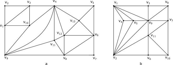
Figure 2: (a) Edges $(v_{1},v_{3})$, $(v_{6},v_{8})$ and $(v_{4},v_{9})$ are shortcuts. $v_{1}v_{2}v_{3}$ and $v_{6}v_{7}v_{8}$ are CIPs and (b) $\triangle v_{1}v_{2}v_{9}$ is a separating triangle

Theorem 2.1.

[3, Theorem 3] A nonseparable plane graph $\mathcal{G}$ with triangular interior faces (regions) is an RDG if and only if it has at most 4 CIPs and has no separating triangle.

The graph shown in Fig. 2a is an RDG while the graph in Fig. 2b is not an RDG because of the presence of a separating triangle.

Theorem 2.2.

[3, Theorem 5] A separable connected plane graph $\mathcal{G}$ with triangular interior faces (regions) is an RDG if and only if

1. $\mathcal{G}$ has no separating triangle,

2. BNG of $\mathcal{G}$ is a path,

3. each maximal block corresponding to the endpoints of the BNG contains at most 2 critical CIPs,

4. no other maximal block contains a critical CIP.

3 Introduction to an MRDG and an edge-reducible RDG

In this section, we introduce an MRDG and some important properties of the MRDG. Further we also introduce an edge-reducible RDG.

Definition 3.1.

An RDG $\mathcal{G}=(V,E)$ is called maximal RDG (MRDG) if there does not exist an RDG $\mathcal{G^{\prime}}=(V,E^{\prime})$ with $E^{\prime}\supset E$.

Definition 3.2.

An RDG $\mathcal{G}=(V,E)$ is said to be edge-reducible if there exists an RDG $\mathcal{G^{\prime}}=(V,E^{\prime})$ such that $E\supset E^{\prime}$. If an RDG is not edge-reducible, it is said to be an edge-irreducible RDG.

For a better understanding of Definitions 3.1 and 3.2, refer to Fig. 3. In Fig. 3a, the given RDG is an MRDG since adding a new edge to it, its exterior becomes triangular and hence one of the exterior modules in its floorplan will be non-rectangular. The corresponding RFP of the MRDG is shown in 3b where $R_{i}$ corresponds to $v_{i}$. In Fig. 3c, the given graph $\mathcal{G}$ is an edge-irreducible biconnected RDG since after removing an edge from it, it no longer remains an RDG. In fact, on removing an exterior edge from $\mathcal{G}$, it transforms to a separable connected graph where one of its blocks contains three critical CIPs. It is noted that we can not remove an interior edge from $\mathcal{G}$ since the resultant graph must have triangular interior regions. This is because we only consider plane graphs with triangular interior regions.

Theorem 3.1.

The number of edges in an MRDG is $2n-2$ or $3n-7$ where $n$ denotes the number of vertices in the MRDG.

Proof.

Let $\mathcal{M}$ be an MRDG with $n$ vertices. If $d(v_{i})=n-1$ for some vertex $v_{i}\in\mathcal{M}$, then clearly it is a wheel graph $W_{n}$. $W_{n}$ is independent of separating triangle and CIP. By Theorem 2.1, it is an RDG. Note that adding a new edge to $W_{n}$ creates a separating triangle passing through its central vertex and two of its exterior vertices. This implies that it is maximal RDG. Now by degree sum formula, the sum of degree of all vertices of a graph is twice of the number of its edges. This implies that $3(n-1)+(n-1)=2$(the number of edges in $W_{n}$) and hence the number of edges in $W_{n}$ is $2n-2$.

We have shown that $W_{n}$ is an MRDG with $2n-2$ edges and in this case, the number of edges in $\mathcal{M}$ is $2n-2$.

Now suppose that $d(v_{i})<n-1,\leavevmode\nobreak\ \forall\leavevmode\nobreak\ v_{i}\leavevmode\nobreak\ \in\mathcal{M}$. Consider a maximal plane graph $\mathcal{G}$ with $n$ vertices such that there does not exist any separating triangle in its interior. We claim that $\mathcal{M}=\mathcal{G}-(v_{i},v_{j})$ for some exterior edge $(v_{i},v_{j})$ of $\mathcal{G}$. In order to claim this, we need to show that $\mathcal{G}-(v_{i},v_{j})$ is an MRDG with $3n-7$ edges.

By our assumption on $\mathcal{G}$, it is evident that $\mathcal{G}-(v_{i},v_{j})$ has no separating triangle. Suppose that $\mathcal{G}-(v_{i},v_{j})$ has a CIP. Then there is a shortcut $(v_{s},v_{t})$ in $\mathcal{G}-(v_{i},v_{j})$. This implies that $\mathcal{G}$ has a separating triangle $v_{s}v_{t}v_{e}$ in its interior where $v_{e}$ is its exterior vertex. This is a contradiction to our assumption that $\mathcal{G}$ has no separating triangle in its interior. Thus we see that $\mathcal{G}-(v_{i},v_{j})$ has no CIP. Thus By Theorem 2.1, it is an RDG.

The number of edges in a maximal plane graph is $3n-6$. This implies that $\mathcal{G}-(v_{i},v_{j})$ has $3n-7$ edges. Note that adding a new edge to $\mathcal{G}-(v_{i},v_{j})$, creates a separating triangle in $\mathcal{G}-(v_{i},v_{j})$ and hence it is an MRDG.

Thus we see that $\mathcal{G}-(v_{i},v_{j})$ is an RDG with $3n-7$ edges and hence $\mathcal{M}$ is an MRDG with $3n-7$ edges.

∎

Theorem 3.2.

The number of vertices on the outermost cycle of an MRDG with $n$ vertices is $4$ or $n-1$.

Proof.

Let $\mathcal{M}$ be an MRDG with $n$ vertices. If $\mathcal{M}$ is a wheel graph $W_{n}$, then it is clear that it has $n-1$ vertices on its exterior. Otherwise it is obtained from a maximal plane graph that has no separating triangle in its interior by deleting one of its exterior edges. But a maximal plane graph has 3 vertices on its exterior. Then it is evident that $\mathcal{M}$ has 4 vertices on its exterior. ∎

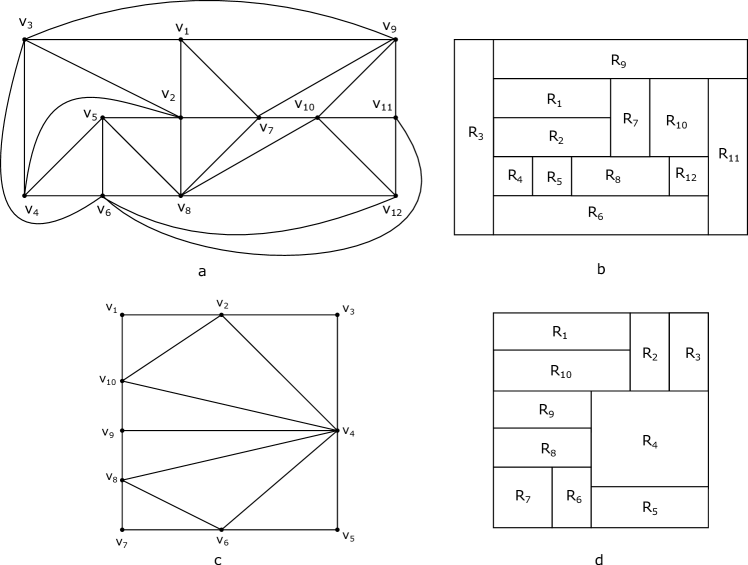
Figure 3: (a-b) An MRDG and its RFP, and (c-d) an edge-irreducible biconnected RDG and its RFP.

4 MRDG Construction

In this section, we first prove that it is always possible to construct an MRDG $\mathcal{M}=(V,E)$ for a given RDG $\mathcal{G}=(V,E_{1})$ such that $E_{1}\subset E$. Then we present an algorithm for its construction corresponding to $\mathcal{G}$.

In order to prove the main result, we first need to prove some lemmas. Denote $|N(v_{i})\cap N(v_{j})|$ by $s$ for any two adjacent vertices $v_{i}$ and $v_{j}$ of an RDG $\mathcal{G}$.

Lemma 4.1.

If $s=0$ , then $(v_{i},v_{j})$ is an exterior edge of $\mathcal{G}$.

Proof.

For $s=0$, $(v_{i},v_{j})$ is a cut-edge (bridge) and hence is an exterior edge. ∎

Lemma 4.2.

For all adjacent vertices $v_{i}$ and $v_{j}$, $s\leq 2$.

Proof.

To the contrary, suppose that $s=3$. Consider a plane embedding $\mathcal{G}_{e}$ of $\mathcal{G}$. Since, $s=3$, $N(v_{i})$ and $N(v_{j})$ must have 3 common vertices $v_{k}$, $v_{l}$ and $v_{m}$ which results in 3 cycles $v_{i}v_{j}v_{k}$, $v_{i}v_{j}v_{l}$ and $v_{i}v_{j}v_{m}$ in $\mathcal{G}_{e}$. Now $(v_{i},v_{j})$ is a common edge in these 3 cycles. This implies that atleast 2 of 3 cycles would lie on the same side of $(v_{i},v_{j})$ in $\mathcal{G}_{e}$. This means that one of the cycles encloses some vertex $v_{t}$ of the other cycle and hence is not a face in $\mathcal{G}_{e}$. Therefore its removal results $\mathcal{G}_{e}$ in a disconnected graph and hence it is a separating triangle in $\mathcal{G}$, which is a contradiction to Theorems 2.1 and 2.2 since $\mathcal{G}$ is an RDG. Similarly, if $s\geq 3$, we arrive at the contradiction. ∎

Lemma 4.3.

$(v_{i},v_{j})$ is an interior edge of $\mathcal{G}$ if and only if $s=2$.

Proof.

First suppose that $s=2$. We need to show that $(v_{i},v_{j})$ is an interior edge in $\mathcal{G}$. To the contrary, suppose that $(v_{i},v_{j})$ is an exterior edge of $\mathcal{G}$. Let $N(v_{i})\cap N(v_{j})=\{v_{k},v_{l}\}$. Since $(v_{i},v_{j})$ is an exterior edge, there exist two triangles $v_{i}v_{j}v_{k}$, $v_{i}v_{j}v_{l}$ in the plane embedding of $\mathcal{G}$ such that both lie on the same side of $(v_{i},v_{j})$. This implies that one of them contains the other and hence is not a region (face) and is a separating triangle. This is a contradiction to Theorems 2.1 and 2.2 since $\mathcal{G}$ is an RDG.

Conversely, suppose that $(v_{i},v_{j})$ is an interior edge in $\mathcal{G}$. Since $\mathcal{G}$ is an RDG, each of its interior regions is triangular. This implies that there exist two triangles $v_{i}v_{j}v_{k}$ and $v_{i}v_{j}v_{l}$ in the plane embedding of $\mathcal{G}$. Hence $N(v_{i})$ and $N(v_{j})$ have atleast two vertices in common, i.e., $s\geq 2$. By Lemma 4.2, we have $s\leq 2$. Hence $s=2$. ∎

Corollary 4.1.

If $s=1$, then $(v_{i},v_{j})$ is an exterior edge of $\mathcal{G}$.

Proof.

It is the direct consequence of Lemmas 4.1 and 4.3. ∎

Lemma 4.4.

It is always possible to construct a nonseparable (biconnected) RDG from a separable connected RDG by adding edges to it.

Proof.

Let $\mathcal{G}_{1}=(V,E_{1})$ be a separable connected RDG such that it has atleast one bridge (cut-edge). Suppose that $L_{1}=\{(v_{i},v_{j})\in E_{1}\leavevmode\nobreak\ |\leavevmode\nobreak\ \leavevmode\nobreak\ |N(v_{i})\cap N(v_{j})|=0\}$ and $L_{2}=\{(v_{a},v_{b})\in E_{1}\leavevmode\nobreak\ |\leavevmode\nobreak\ \leavevmode\nobreak\ |N(v_{a})\cap N(v_{b})|=1\}$. Consider two adjacent edges, $(v_{i},v_{j})$ from $L_{1}$ and $(v_{j},v_{k})$ from $L_{2}$ such that $|N(v_{i})\cap N(v_{k})|=1$. Such selection is always possible since both edges belongs to different blocks and $N(v_{i})\cap N(v_{k})=\{v_{j}\}$.

Construct a graph $\mathcal{G}_{2}=(V,E_{2})$ where $E_{2}=E_{1}\cup\{(v_{i},v_{k})\}$. To prove $\mathcal{G}_{2}$ is an RDG, we prove the following:

• there does not exist a separating triangle passing through $(v_{i},v_{k})$ in $\mathcal{G}_{2}$

  There would be a separating triangle passing through $(v_{i},v_{k})$ in $\mathcal{G}_{2}$ if $|N(v_{i})\cap N(v_{k})|=2$ in $\mathcal{G}_{2}$. In this case, $v_{j},v_{r}\in N(v_{i})\cap N(v_{k})$ such that $v_{r}$ lies inside the triangle passing through $(v_{i},v_{k})$. But $(v_{i},v_{j})\in L_{1}$ and $(v_{j},v_{k})\in L_{2}$. Therefore by Lemma 4.1 and Corollary 4.1, both $(v_{i},v_{j})$ and $(v_{j},v_{k})$ are the exterior edges and $v_{i}$ and $v_{k}$ belongs to different blocks in $\mathcal{G}_{1}$. Hence in $\mathcal{G}_{2}$, $|N(v_{i})\cap N(v_{k})|=1$ is the only possibility.

• the number of critical CIPs in $\mathcal{G}_{2}$ can not exceed the number of critical CIPs in $\mathcal{G}_{1}$

  In $\mathcal{G}_{2}$, a critical CIP can only pass through $(v_{i},v_{k})$, which already passes through $(v_{i},v_{j})$ and $(v_{j},v_{k})$ in $\mathcal{G}_{1}$. But $v_{j}$ is a cut vertex which is a contradiction to the fact that a critical CIP never passes through a cut vertex.

Since $\mathcal{G}_{1}$ is an RDG, each of its region is triangular. The new edge $(v_{i},v_{k})$ is added with the property that $|N(v_{i})\cap N(v_{k})|=1$. By Corollary 4.1, $(v_{i},v_{k})$ is exterior edge in $\mathcal{G}_{2}$. Therefore, the new region $v_{i}v_{j}v_{k}$ is triangular in $\mathcal{G}_{2}$. By Theorem 2.2, $\mathcal{G}_{2}$ is an RDG.

After adding $(v_{i},v_{k})$ to $\mathcal{G}_{1}$, the edge $(v_{i},v_{j})$ from $L_{1}$ belongs to $L_{2}$ since $|N(v_{i})\cap N(v_{j})|=1$ ($|N(v_{i})\cap N(v_{j})|=\{v_{k}\}$). Therefore a recursive process shows that at the iteration until $L_{1}$ is empty, $\mathcal{G}_{k+1}=(V,E_{k+1})$ becomes a separable connected RDG with cut-vertices (vertex), but no cut edge where $E_{k+1}=E_{k}\cup(v_{a},v_{c})$ such that $(v_{a},v_{b})$ is from $L_{1}$ and $(v_{b},v_{c})$ is from $L_{2}$ with the property $|N(v_{a})\cap N(v_{c})|=1$. In this way, we can construct a separable connected RDG having cut-vertices of the given separable connected RDG only.

It now remains to show that it is always possible to construct a nonseparable (biconnected) RDG of the given separable connected RDG $\mathcal{G}_{1}=(V,E_{1})$ having cut-vertices but no cut-edges. Let $v_{t}$ be its cut-vertex. Since it has no cut-edge, $d(v_{t})\geq 4$. A plane embedding of $\mathcal{G}_{1}$ with exterior cycles $C_{1}$ and $C_{2}$ sharing a cut vertex $v_{t}$ is shown in Fig. 5a. It is evident from this embedding that there is no separating triangle passing though the new added edges (red edges) in the resultant graph shown in Fig. 5b. Since $v_{t}$ is a cut-vertex, none of the vertices $v_{1}$, $v_{2}$, $v_{3}$ and $v_{4}$ in Fig. 5, which are adjacent to $v_{t}$, can be the endpoints of a shortcut in $\mathcal{G}_{1}$. This implies that the number of CIPs in the resultant graph (shown in Fig. 5b) can not exceed than the number of critical CIPs in $\mathcal{G}_{1}$. This proves the required result. ∎

Figure 4: (a) A random addition of new edges (red edges) to a separable connected RDG destroy the RDG property because of generating a separating triangle $v_{4}v_{5}v_{7}v$ in the resultant graph (b) while adding new edges (red edges) by Lemma 4.4 do not destroy RDG property ( no separating triangle and any CIP in the resultant graph).

Remark 4.1.

It is not straight forward to add edges to a separable connected RDG maintaining RDG property. Randomly adding new edges to an RDG can destroy the RDG property, i.e., can produce either a CIP or a separating triangle in the resultant graph. In the lie of this, we have shown the procedure of adding edges by Lemma 4.4. For instance, consider a separable connected RDG shown in Fig. 4a. It is transformed to a nonseparable graph by adding new edges (red edges) randomly. As a result, the nonseparable graph thus obtained is not an RDG. In fact, it contains a separating triangle $v_{4}v_{5}v_{7}$. On the other hand, red edges are added to the same graph by using Lemma 4.4 in order to construct a nonseparable RDG shown in Fig. 4b. Thus Lemma 4.4 is helpful in introducing pattern of new edges to be added to a separable connected RDG to be a nonseparable RDG.

Figure 5: Constructing a nonseparable RDG of a separable connected RDG $\mathcal{G}_{1}$ with a cut-vertex $v_{t}$ shared by its two components $C_{1}$ and $C_{2}$.

Lemma 4.5.

It is always possible to construct an MRDG from a biconnected RDG by adding edges to it.

Proof.

Let $\mathcal{G}_{1}=(V,E_{1})$ be a biconnected RDG. If $|E_{1}|=3|V|-7$ or $\mathcal{G}_{1}=W_{n}$, then $\mathcal{G}_{1}$ is itself an MRDG and the proof is obvious.

Suppose that $|E_{1}|<(3|V|-7)$ and $\mathcal{G}_{1}\neq W_{n}$. Assume that $L_{2}=\{(v_{i},v_{j})\in E_{1}\mid|N(v_{i})\cap N(v_{j})|=1\}$. By Lemma 4.1, $L_{2}$ is a list of all exterior edges of $\mathcal{G}_{1}$.

We now prove that there exists atleast a pair of adjacent edges $(v_{i},v_{j})$ and $(v_{j},v_{k})$ in $L_{2}$ such that $|N(v_{i})\cap N(v_{k})|=1$. If such pair does not exist, then $|N(v_{a})\cap N(v_{c})|=2$ for each pair $(v_{a},v_{b})$ and $(v_{b},v_{c})$ in $L_{2}$. In fact, since $\mathcal{G}_{1}$ is a biconnected graph, by Lemma 4.2, we have $|N(v_{a})\cap N(v_{c})|\in\{1,2\}$. Let $v_{1}v_{2}\dots v_{p}$ be the outermost cycle of $\mathcal{G}_{1}$. Note that all edges $(v_{1},v_{2})$, $(v_{2},v_{3})$ …$(v_{p-1},v_{p})$ and $(v_{p},v_{1})$ are exterior and hence by Lemma 4.2, all these edges belongs to $L_{2}$. Now if we choose $(v_{1},v_{2})$ and $(v_{2},v_{3})$, then $|N(v_{1})\cap N(v_{3})|=\{v_{2},v_{c}\}$. Again if we choose $(v_{2},v_{3})$ and $(v_{3},v_{4})$, then $|N(v_{2})\cap N(v_{4})|=\{v_{3},v_{c}\}$. Continuing in this way, we see that all the exterior vertices are adjacent to $v_{c}$. Observe that the vertex $v_{c}$ and every adjacent exterior vertices $v_{i}$ and $v_{j}$ forms a triangle. Therefore, if $\mathcal{G}_{1}$ has any other vertex (except $v_{1},v_{2},\dots,v_{p}$ and $v_{c}$ ), it would lie inside the triangle $v_{i}v_{j}v_{c}$, which is a separating triangle. This contradicts the fact that $\mathcal{G}_{1}$ is an RDG. This implies that $\mathcal{G}_{1}$ cannot have any other vertex (except $v_{1},v_{2},\dots,v_{p}$ and $v_{c}$) which concludes that $\mathcal{G}_{1}$ is a wheel graph $W_{n}$ which is again a contradiction since we assumed that $\mathcal{G}_{1}\neq W_{n}$. This proves our claim.

Choose two adjacent edges $(v_{i},v_{j})$ and $(v_{j},v_{k})$ from $L_{2}$ such that $|N(v_{i})\cap N(v_{k})|=1$ and construct a graph $\mathcal{G}_{2}=(V,E_{2})$ where $E_{2}=E_{1}\cup\{(v_{i},v_{k})\}$.

Now we show that the number of CIPs in $\mathcal{G}_{2}$ can not exceed the number of CIPs in $\mathcal{G}_{1}$. For $\mathcal{G}_{2}$, there are the following possibilities:

1. None of vertices $v_{i}$ and $v_{k}$ is the endpoint of a shortcut in $\mathcal{G}_{1}$,

2. One of vertices $v_{i}$ and $v_{k}$ is the endpoint of a shortcut in $\mathcal{G}_{1}$,

3. Both vertices $v_{i}$ and $v_{k}$ are the endpoints of a shortcut in $\mathcal{G}_{1}$.

These 3 possibilities are shown in Fig. 6a-6c respectively. In the first case, clearly there is no CIP passing through $(v_{i},v_{k})$ in $\mathcal{G}_{2}$. In the second case, $v_{i}v_{k}v_{k+1}\dots v_{q-1}v_{q}$ becomes a CIP in $\mathcal{G}_{2}$ and $v_{i}v_{j}v_{k}v_{k+1}\dots v_{q-1}v_{q}$ no longer remains a CIP in $\mathcal{G}_{2}$. In fact, the edges $(v_{i},v_{j})$ and $(v_{j},v_{k})$ of the existing CIP in $\mathcal{G}_{1}$ are replaced by $(v_{i},v_{k})$ in $\mathcal{G}_{2}$. Thus, in this case, the number of CIPs do not get increased. The third case is not possible since $|N(v_{i})\cap N(v_{k})|=2$. In fact, $N(v_{i})\cap N(v_{k})=\{v_{j},v_{s}\}$ and $\mathcal{G}_{2}$ is obtained from $\mathcal{G}_{1}$ by adding an edge $(v_{i},v_{k})$ such that $|N(v_{i})\cap N(v_{k})|=1$. This proves our claim.

Now we claim that there does not exist a separating triangle passing through $(v_{i},v_{k})$ in $\mathcal{G}_{2}$. Since $|N(v_{i})\cap N(v_{k})|=1$, i.e., $N(v_{i})\cap N(v_{k})=\{v_{j}\}$. Therefore $v_{i}v_{j}v_{k}$ is the only cycle of length 3 having no vertex inside and passing through $(v_{i},v_{k})$ in $\mathcal{G}_{2}$. This shows that $v_{i}v_{j}v_{k}$ is not a separating triangle, it is a new added triangular region (face) in $\mathcal{G}_{2}$. By Theorem 2.1, $\mathcal{G}_{2}$ is an RDG. A recursive process shows that each $\mathcal{G}_{i}=(V,E_{i})$, $(i\geq 3)$ is an RDG where $E_{i}=E_{i-1}\cup\{(v_{a},v_{c})\}$ such that $|N(v_{a})\cap N(v_{c})|=1$ for some edges $(v_{a},v_{b}),(v_{b},v_{c})$ belong to $L_{2}$ which is defined as $L_{2}=\{(v_{i},v_{j})\in E_{i-1}\mid|N(v_{i})\cap N(v_{j})|=1\}$.

It can be noted that the recursive process will terminate when the outermost cycle has four vertices for some RDG $\mathcal{G}_{k}$. In fact, $(v_{i},v_{j})$, $(v_{j},v_{k})$, $(v_{k},v_{l})$ and $(v_{l},v_{i})$ are four edges constituted by the four exterior vertices $v_{i}$, $v_{j}$, $v_{k}$ and $v_{l}$ of some RDG $\mathcal{G}_{k}$. For any two edges $(v_{a},v_{b})$ and $(v_{b},v_{c})$, we have $|N(v_{a})\cap N(v_{c})|=2$. This terminate our process. On the other hand, there does not exist any other way for adding a new edge such that the resultant graph is an RDG with a new triangular region. Recall that a maximal plane graph has $3|V_{1}|-6$ edges where $V_{1}$ denotes its vertex set and has all triangular regions including exterior. In our case, every region of $\mathcal{G}_{k}$ is triangular, but exterior is quadrangle. This implies that the number of edges in $\mathcal{G}_{k}$ is $3|V|-7$ and hence it is an MRDG. This completes the proof of lemma. ∎

From Lemmas 4.4-4.5, we conclude that the following main result of the paper.

Theorem 4.1.

It is always possible to construct an MRDG of a given RDG.

Algorithm 1 Constructing an MRDG of a given RDG

0:  An RDG $\mathcal{G}_{1}=(V,E_{1})$

0:  An MRDG $\mathcal{M}=(V,E)$ for $\mathcal{G}=(V,E_{1})$ such that $|E_{1}|<|E|$

1:  $L_{1}\leftarrow\phi$

2:  $L_{2}\leftarrow\phi$

3:  for all $(v_{i},v_{j})\in E_{1}$ do

4:     $s\leftarrow|N(v_{i})\cap N(v_{j})|$

5:     if $s==0$ then

6:        $L_{1}\leftarrow L_{1}\cup\{(v_{i},v_{j})\}$

7:     else if $s==1$ then

8:        $L_{2}\leftarrow L_{2}\cup\{(v_{i},v_{j})\}$

9:     else

10:        continue

11:     end if

12:  end for

13:  for all $(v_{i},v_{j})\in L_{1}$ do

14:     if $(v_{j},v_{k})\in L_{2}$ then

15:        $L_{2}\leftarrow(L_{2}\cup\{(v_{i},v_{j}),(v_{i},v_{k})\})-\{(v_{j},v_{k})\}$

16:        $E_{1}\leftarrow E_{1}\cup\{(v_{i},v_{k})\}$

17:     else

18:        continue

19:     end if

20:  end for

21:  for all $(v_{i},v_{j}),(v_{j},v_{k})\in L_{2}$ do

22:     if $|N(v_{i})\cap N(v_{k})|==1$ then

23:        $L_{2}\leftarrow L_{2}\cup\{(v_{i},v_{k})\}-\{(v_{i},v_{j}),(v_{j},v_{k})\}$

24:        $E_{1}\leftarrow E_{1}\cup\{(v_{i},v_{k})\}$

25:     else

26:        continue

27:     end if

28:  end for

29:  for all $(v_{i},v_{j})\in E_{1}$ do

30:     if $(v_{i},v_{j})\in(E_{1}-\{(v_{i},v_{j})\})$ then

31:        $E_{1}\leftarrow E_{1}-\{(v_{i},v_{j})\}$

32:     else

33:        continue

34:     end if

35:  end for

36:  return  $\mathcal{G}$

Since the output of Algorithm 1 is an MRDG having four vertices on its exterior, the corresponding RFP would have four rectangles on the exterior. It may not always be desirable to transform a given RDG to an MRDG. In such a case, we can replace $L_{2}$ by $L_{2}-A$ where $A$ is the set of edges not to be added to the given RDG. Thus we can obtain the required RDG from a given RDG.

For a better understanding to Algorithm 1, we explain its steps through an example. Consider an RDG $\mathcal{G}_{1}=(V,E_{1})$ shown in Fig. 7a. First of all, Algorithm 1 computes two sets $L_{1}$ and $L_{2}$ (the lines $3-12$) from $\mathcal{G}_{2}$ such that $L_{1}$ contains those edges whose endpoints have no common vertex and $L_{2}$ contains those edges whose endpoints have exactly one common vertex. Then $L_{1}=\{(v_{7},v_{10})\}$ and $L_{2}=\{(v_{1},v_{2})$, $(v_{2},v_{3}),$ $(v_{3},v_{4}),$ $(v_{4},v_{6}),$ $(v_{6},v_{8}),$ $(v_{7},v_{8}),$ $(v_{10},v_{12}),$ $(v_{11},v_{12},(v_{9},v_{11}),$ $(v_{9},v_{10}),$ $(v_{7},v_{1})\}$.

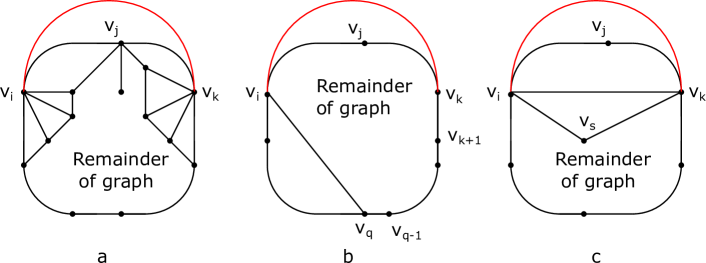
Figure 6: Three possible depictions of $\mathcal{G}_{2}$ obtained from $\mathcal{G}_{1}$ (consists of black edges) by adding a red edge.

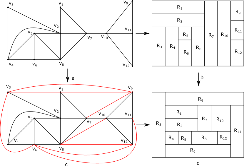
Figure 7: A given RDG $\mathcal{G}_{1}$ and (b) its RFP, (c) the derivation of an MRDG $\mathcal{M}_{2}$ from $\mathcal{G}_{1}$, and (d) its RFP.

Now it executes the rest of its steps ( $13-20$) as follows:

Since for $(v_{7},v_{10})\in L_{1}$, there is an edge $(v_{10},v_{9})$ belonging to $L_{2}$, the loop ($13-20$) adds $(v_{7},v_{9})$ and $(v_{7},v_{10})$ to $L_{2}$, and adds $(v_{7},v_{9})$ to $E_{1}$. Further, it subtracts $(v_{10},v_{9})$ from $L_{2}$. Thus, $L_{2}=\{(v_{7},v_{10}),$ $(v_{7},v_{9}),$ $(v_{1},v_{2})$, $(v_{2},v_{3}),$ $(v_{3},v_{4}),$ $(v_{4},v_{6}),$ $(v_{6},v_{8}),$ $(v_{7},v_{8}),$ $(v_{10},v_{12}),$ $(v_{11},v_{12},(v_{9},v_{11}),$ $(v_{7},v_{1})\}$ and $E_{1}=E_{1}\cup\{(v_{7},v_{9})\}$. Since $L_{1}$ has exactly one edge, this loop terminates (In fact, we have transformed the given separable connected RDG to an nonseparable RDG. This method was proved by Lemma 4.4) and Algorithm 1 executes the next loop ($21-28$) as follows:

Suppose that Algorithm 1 picks $(v_{9},v_{7})$ and $(v_{7},v_{1})$ from $L_{2}$. Since $N(v_{1})\cap N(v_{9})=\{v_{7}\}$, $|N(v_{1})\cap N(v_{9})|=1$. Then it subtracts $(v_{9},v_{7})$ and $(v_{7},v_{1})$ from $L_{2}$ and adds $(v_{9},v_{1})$ to both $L_{2}$ and $E_{1}$ ( the lines 23 and 24). Thus $L_{2}=\{(v_{9},v_{1}),$ $(v_{7},v_{10}),$ $(v_{1},v_{2})$, $(v_{2},v_{3}),$ $(v_{3},v_{4}),$ $(v_{4},v_{6}),$ $(v_{6},v_{8}),$ $(v_{7},v_{8}),$ $(v_{10},v_{12}),$ $(v_{11},v_{12},(v_{9},v_{11})\}$ and $E_{1}=E_{1}\cup\{(v_{9},v_{1}),(v_{7},v_{9})\}$.

Again it picks $(v_{10},v_{7})$ and $(v_{7},v_{8})$ from $L_{2}$. Since $N(v_{10})\cap N(v_{8})=\{v_{7}\}$, $|N(v_{10})\cap N(v_{8})|=1$, it subtracts $(v_{10},v_{7})$ and $(v_{7},v_{8})$ from $L_{2}$, and adds $(v_{10},v_{8})$ to both $L_{2}$ and $E_{1}$ (the lines 23 and 24).Thus, $L_{2}=\{(v_{10},v_{8}),$ $(v_{9},v_{1}),$ $(v_{1},v_{2})$, $(v_{2},v_{3}),$ $(v_{3},v_{4}),$ $(v_{4},v_{6}),$ $(v_{6},v_{8}),$ $(v_{10},v_{12}),$ $(v_{11},v_{12},(v_{9},v_{11})\}$ and $E_{1}=E_{1}\cup\{(v_{10},v_{8}),$ $(v_{9},v_{1}),(v_{7},v_{9})\}$.

Thus a recursive process of this loop adds $\{(v_{6},v_{11}),$ $(v_{3},v_{6}),$ $(v_{9},v_{3}),$ $(v_{9},v_{11})\}$ to $L_{2}$ and $E_{1}=E_{1}\cup\{(v_{9},v_{3}),$ $(v_{6},v_{12}),$ $(v_{8},v_{12}),$ $(v_{3},v_{6}),$ $(v_{9},v_{3}),$ $(v_{8},v_{10}),$ $(v_{9},v_{1}),$ $(v_{3},v_{1}),$ $(v_{9},v_{7})\}$ respectively.

Since there has not been added any duplicate edge (multiple edges), the loop ($30-35$) skips automatically.

Thus we see that the output is an MRDG $\mathcal{M}_{2}$ shown in Fig. 7c where red edges are the new edges which are added to $\mathcal{G}_{1}$. Note that $\mathcal{G}_{1}$ admits an RFP $\mathcal{F}_{1}$ shown in 7b and $\mathcal{M}_{2}$ admits an RFP $\mathcal{F}_{2}$ shown in 7d. Consequently to this, $\mathcal{F}_{1}$ can be transformed to $\mathcal{F}_{2}$ (a maximal one).

Analysis of computational complexity

Let $v_{s}$ be a vertex of the largest degree in the input RDG $\mathcal{G}$. This implies that $|N(v_{i}|\leq K$ where $d(v_{s})=K$. Now we consider each of the following loops:

1. The computational complexity of the lines $3-12$ is $(|N(v_{i})||N(v_{j})||E_{1}|)\cong K^{2}|E_{1}|\cong$ O$(n)$.

2. The computational complexity of the lines $14-20$ is $(|L_{1}|.|L_{2}|)\cong|L_{2}|\cong$ O$(n)$. In fact, $L_{1}$ contains edges whose endpoints are cut vertices. $|L_{1}|\cong$ O$(n)$ if the given RDG is a path graph. In that case, $L_{2}$ is empty. Both $L_{1}$ and $L_{2}$ can not be large simultaneously.

3. The computational complexity of the lines $21-28$ is $(|N(v_{i})||N(v_{j})|+|L_{2}|)|L_{2}|$ $\cong K^{2}|L_{2}|^{2}\cong$ O$(n^{2})$.

4. The computational complexity of the lines $29-35$ is $|E_{1}|^{2}\cong$ O$(n^{2})$.

Hence, the computational complexity of Algorithm 1 is quadratic.

Remark 4.2.

If $|N(v_{i})|$ or $|N(v_{j})|$ or $|N(v_{i})|\times|N(v_{i})|$ is near to $|V|$, then the computational complexity of Algorithm 1 becomes O$(n^{3})$. However, in design problems such graphs do not appears quite often. Both $|N(v_{i})|$ and $|N(v_{j})|$ can not be near to $|V|$ in a plane graph.

5 Reduction Method

In this section, we show that an edge-reducible biconnected RDG can always be transformed to an edge-irreducible biconnected RDG. Then we present Algorithm 2 that computes the number of CIPs in a given RDG which is a further input requirement for Algorithm 3 as a call function. Algorithm 3 transforms an edge- reducible biconnected RDG to an edge-irreducible biconnected RDG.

Theorem 5.1.

If an RDG $\mathcal{G}=(V,E)$ is edge-reducible to an RDG $\mathcal{G}^{\prime}=(V,E)$ such that $E=E^{\prime}\cup\{(v_{i},v_{j})\}$, then $(v_{i},v_{j})$ is an exterior edge of $\mathcal{G}$.

Proof.

Assume that $C$ and $C^{\prime}$ be the exterior faces of $\mathcal{G}$ and $\mathcal{G}^{\prime}$ respectively. Since both $\mathcal{G}$ and $\mathcal{G}^{\prime}$ are RDGs, each interior face of both $\mathcal{G}$ and $\mathcal{G}^{\prime}$ are of equal length ( i.e., of length 3). But $E^{\prime}\subsetneq E$ and, $\mathcal{G}$ and $\mathcal{G}^{\prime}$ have the same number of vertices. This implies that $C$ and $C^{\prime}$ have different length, i.e., $|C|<|C^{\prime}|$. Also, when $(v_{i},v_{j})$ is removed from $C$, the two other edges of the triangle passing through $(v_{i},v_{j})$ becomes a part of $C^{\prime}$, i.e., removing an edge from $C$ increases the size of $C^{\prime}$ by one. Thus we see that $|C^{\prime}|-|C|=1$ and $(v_{i},v_{j})$ belongs to $C$. Hence $(v_{i},v_{j})$ is an exterior edge of $\mathcal{G}$. ∎

Theorem 5.1 suggests us that an edge-reducible RDG can be transformed to any other RDG by deleting some of its exterior edges. Then further such resultant RDG can also be transformed to another RDG by deleting some of its exterior edges. Such recursion process can be continued until the graph remains an RDG. Following this, now we are going to prove another main result of this paper.

Theorem 5.2.

It is always possible to transform an edge-reducible biconnected RDG to an edge-irreducible biconnected RDG.

Proof.

Let $\mathcal{G}_{1}=(V,E_{1})$ be an edge-reducible biconnected RDG. Let $Z_{1}$ be the set of all exterior edges of $\mathcal{G}_{1}$. If for each edge $(v_{i},v_{j})\in Z_{1}$, $|N(v_{i})|\leq 2$ or $|N(v_{j})|\leq 2$, then $\mathcal{G}_{1}=(V,E_{1})$ is an edge-irreducible biconnected RDG which is a contradiction. This implies we can select an edge $(v_{i},v_{j})$ from $Z_{1}$ such that $|N(v_{i})|>2,|N(v_{j})|>2$. And construct a nonseparable graph $\mathcal{G}_{2}=(V,E_{2})$ with atmost 4 CIPs where $E_{2}=E_{1}-\{(v_{i},v_{j})\}$. Such a nonseparable graph always exists otherwise it has more than four CIPs, $\mathcal{G}_{1}$ becomes an edge-irreducible RDG which contradicts our assumption. Since $(v_{i},v_{j})$ is an exterior edge and $\mathcal{G}_{1}=(V,E_{1})$ is a biconnected RDG, $|N(v_{i})\cap N(v_{j})|=1$. Suppose that $(N(v_{i})\cap N(v_{j}))=\{v_{t}\}$.

Now we claim that $\mathcal{G}_{2}$ is an RDG. Since $\mathcal{G}_{1}$ is an RDG, each of its interior regions are triangular. On removing an exterior edge from an RDG, the remaining interior regions remains triangular. This implies that each interior region of $\mathcal{G}_{2}$ is triangular. It is evident that the removal of an exterior edge from $\mathcal{G}_{1}$ does not produce a separating triangle. This shows that $\mathcal{G}_{2}$ is independent of separating triangles. Also, by our assumption, $\mathcal{G}_{2}$ has atmost four CIPs. By Theorem 2.1, $\mathcal{G}_{2}$ is a biconnected RDG.

By continuously defining $\mathcal{G}_{k}$ $(k\geq 3)$ as above, a recursive process shows that at the iteration until the above defined conditions remains true, $\mathcal{G}_{k}$ is an edge-reducible biconnected RDG. Hence the proof.

∎

Algorithm 2 NumberOfCIPs($\mathcal{G}=(V,E),W)$

0:  A biconnected RDG $\mathcal{G}=(V,E)$

0:  Number of CIPs in $\mathcal{G}$

1:  $W\leftarrow\phi$, $L\leftarrow\phi$, $U\leftarrow\phi$, $X\leftarrow\phi$

2:  for all $(v_{i},v_{j})\in E$ do

3:     $s\leftarrow|N(v_{i})\cap N(v_{j})|$

4:     if $s==1$ then

5:        $L\leftarrow L\cup\{(v_{i},v_{j})\}$

6:        $U\leftarrow U\cup\{v_{i},v_{j}\}$

7:     else

8:        continue

9:     end if

10:  end for

11:  for all  $(v_{i},v_{j})\in(E-L)$  do

12:     if  $v_{i},v_{j}\in U$  then

13:        $W\leftarrow W\cup\{(v_{i},v_{j})\}$

14:        $X\leftarrow X\cup\{v_{i},v_{j}\}$

15:     else

16:        continue

17:     end if

18:  end for

19:  for all  $(v_{i},v_{j})\in W$  do

20:     if  $(v_{i},v_{i+1}),(v_{i+1},v_{i+2}),\dots,(v_{j-1},v_{j})\in L$ then

21:        if  $v_{k}\in X$, $i+1\leq k\leq j-1$  then

22:           $W\leftarrow W-\{(v_{i},v_{j})\}$

23:        else if $(v_{i},v_{i-1}),(v_{i-1},v_{i-2}),\dots,(v_{j+1},v_{j})\in L$ then

24:           if  $v_{k}\in X$, $i+1\leq k\leq j-1$  then

25:              $W\leftarrow W-\{(v_{i},v_{j})\}$

26:           end if

27:        end if

28:     else

29:        continue

30:     end if

31:  end for

32:  return  $W$

In the most design problems, graphs structures of floorplans are biconnected. Therefore abiding by common design practice, we have described Algorithm 3 for transforming a biconnected RDG to another biconnected RDG.

Algorithm 3 Restoring an edge-reducible biconnected RDG to an edge-irreducible biconnected RDG

0:  A biconnected RDG $\mathcal{G}=(V,E)$

0:  An edge-irreducible biconnected RDG $\mathcal{G}^{\prime}=(V,E^{\prime})$

1:  $Z\leftarrow\phi$

2:  for all $(v_{i},v_{j})\in E$ do

3:     $s\leftarrow|N(v_{i})\cap N(v_{j})|$

4:     if $s==1$ then

5:        $Z\leftarrow Z\cup\{(v_{i},v_{j})\}$

6:     else

7:        continue

8:     end if

9:  end for

10:  for all $(v_{i},v_{j})\in Z$ do

11:     if  $|N(v_{i})|>2\wedge|N(v_{j})|>2\wedge(N(v_{i})\cap N(v_{j}))=\{v_{t}\}$ then

12:        NumberOfCIPs$(\mathcal{G}=(V,E-\{(v_{i},v_{j})\}),W)$

13:        if $|W|\leq 4$ then

14:           $E\leftarrow E-\{(v_{i},v_{j})\}$

15:           $Z\leftarrow Z\cup\{(v_{i},v_{t}),(v_{t},v_{j})\}-\{(v_{i},v_{j})$

16:        else

17:           print  $\mathcal{G}$ is an edge-irreducible biconnected RDG.

18:        end if

19:     end if

20:  end for

21:  return  $\mathcal{G}$

For a better understanding of Algorithm 3, we illustrate its steps through an example. Consider a biconnected RDG $\mathcal{G}_{1}=(V,E_{1})$ shown in Fig. 8a. First of all, the first loop (the lines $3-9$) of Algorithm 3 computes a set $Z$ = $\{(v_{1},v_{3})$, $(v_{1},v_{7}),$ $(v_{5},v_{7}),$ $(v_{3},v_{5})\}$. Now Algorithm 3 executes the steps of second loop (the lines $10-20$) as follows:

Suppose that the second loop picks $(v_{3},v_{5})$ from $Z$ randomly. Then $11^{\text{th}}$ line is executed since $N(v_{3})=4>2$, $N(v_{5})=4>2$ and $N(v_{3})\cap N(v_{5})=\{v_{4}\}$. Next it executes $12^{\text{th}}$ line to determine a set $W$ of CIPs in $\mathcal{G}_{2}=(V,E_{2})$ where $E_{2}=E_{1}-\{(v_{3},v_{5})\}$. Using Algorithm 2, $|W|=0\leq 4$. Then $E_{1}=E_{1}-\{(v_{3},v_{5})\}$ and it adds both $(v_{3},v_{4})$ and $(v_{4},v_{5})$ to $Z$ and remove $(v_{3},v_{5})$ from $Z$. Thus $Z=\{(v_{3},v_{4}),$ $(v_{4},v_{5}),$ $(v_{1},v_{3})$, $(v_{1},v_{7}),$ $(v_{5},v_{7})\}$.

Next suppose that it picks $(v_{1},v_{3})$ from $Z$. Then $11^{\text{th}}$ line is executed since $N(v_{1})=5>2$, $N(v_{3})=4>2$ and $N(v_{1})\cap N(v_{3})=\{v_{2}\}$. Next it executes $12^{\text{th}}$ line to determine the set $W$ for $\mathcal{G}_{3}=(V,E_{3})$ where $E_{3}=E_{2}-\{(v_{1},v_{3})\}$. Using Algorithm 2, we have $W=\{(v_{2},v_{4})\}$, i.e., $|W|=1\leq 4$. Therefore it subtracts $(v_{1},v_{3})$ from both $E_{1}$ and $Z$, and adds both $(v_{1},v_{2})$ and $(v_{2},v_{3})$ to $Z$. Thus $Z=\{(v_{1},v_{2}),$ $(v_{2},v_{3}),$ $(v_{3},v_{4}),$ $(v_{4},v_{5}),$ $(v_{1},v_{7}),$ $(v_{5},v_{7})\}$ and $E_{1}=E_{1}-\{(v_{1},v_{3}),(v_{3},v_{5})\}$.

In this way, the second loop continues until $|W|\leq 4$ with the condition in $11^{\text{t}h}$. Finally we obtain an edge-irreducible biconnected RDG shown in Fig. 8b with the edge set $E-\{(v_{7},v_{9}),$ $(v_{1},v_{9}),$ $(v_{1},v_{7}),$ $(v_{7},v_{5}),$ $(v_{1},v_{3}),$ $(v_{3},v_{5})\}$ and $Z$ (set of the exterior edges) becomes $\{(v_{7},v_{8}),$ $(v_{8},v_{9}),$ $(v_{1},v_{10}),$ $(v_{10},v_{9}),$ $(v_{5},v_{6}),$ $(v_{6},v_{7}),$ $(v_{1},v_{2}),$ $(v_{2},v_{3}),$ $(v_{3},v_{4}),$ $(v_{4},v_{5})\}$.

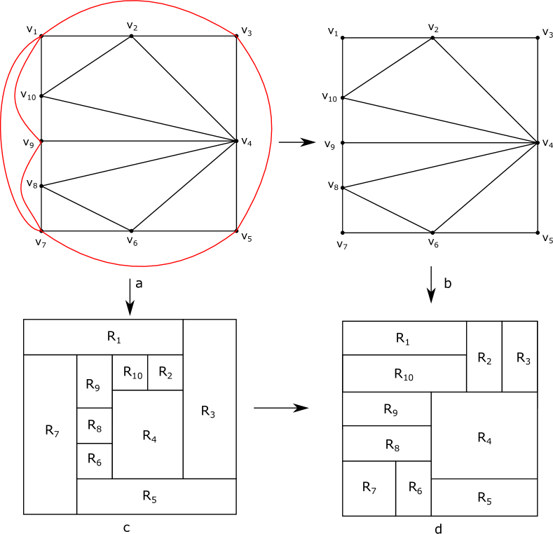
Figure 8: (a) Transformation of an edge-reducible RDG (MRDG) to (b) an edge-irreducible RDG. The respective RFPs are shown in (c) and (d).

It can be noted that the edge-irreducible biconnected RDG in Fig. 8b can not be further transformed to an edge-irreducible separable connected RDG. In fact, the removal of a single edge from it violates RDG property (refer to Theorems 2.1 and 2.2). From this, it follows that a biconnected edge-irreducible RDG may not necessarily be transformed to a separable connected RDG. It may be sometimes possible to restore it to an edge-reducible separable connected RDG by relaxing the conditions $N(v_{i})>2$ and $N(v_{j})>2$ ($11{{}^{\textbf{th}}}$ line). Once if it is transformed to an edge-reducible separable connected RDG, Algorithm 3 can be made applicable for separable connected RDGs with a slight modifications as follows.

Consider a separable connected RDG and construct its BNG. Theorem 2.2 tells us that it is a path. Consider each component corresponding to the vertices of the BNG one by one as an input to Algorithm 3. To proceed, first consider the components corresponding to the initial and end vertices of the BNG as an input to Algorithm 3 and follow Theorem 2.2, i.e., restrict the line 13 of Algorithm 3 by $|W|\leq 2$ such that no CIP should pass through a cut vertex. and restore it to an edge-irreducible one, it is possible using Algorithm 3 since the corresponding block is biconnected. Then, the remaining blocks must be restricted to $|W|=0$ in the line 13 of Algorithm 3. In this way, each biconnected component can be restored to an edge-irreducible one. Finally gluing these edge-irreducible components in the same order as we decomposed them, we obtain an edge-irreducible separable connected RDG from the edge-reducible separable connected RDG.

The ability of Algorithm 3 in the design process is visible as follows.

Algorithm 3 gives an edge-irreducible biconnected RDG as an output for an input biconnected RDG. But it may not be always preferred/required. Of course, one can obtain output as the edge-reducible RDG by imposing some restrictions on $Z$ or $P_{c}$. Suppose that one desires that a particular set $X$ of adjacency relations must not be removed from the given RDG. Then $Z$ or $P_{c}$ (in the lines 10 and 13 respectively) needs to be replaced by $Z-X$ or $P_{c}-X$. This makes Algorithm 3 more practical to design problems. Consequent to this, a particular set of adjacency relations of component rectangles of an existing RFP can be sustained by removing the set $X$ of adjacency relations (edges) of the corresponding vertices in its dual graph as discussed above. Further, Algorithm 3 can give also output as a separable connected RDG for the input biconnected RDG.

Analysis of computational complexity

• The computational complexity of Algorithm 2 is linear

  The computational complexity of the lines $2-10$ is $|N(v_{s})||N(v_{t})||E|=K_{1}K_{2}|E|\cong$ O$(n)$. The computational complexity of the lines $11-18$ is $|U||E-L|\cong$ O$(n)$. The computational complexity of the lines $19-31$ is $|W||L||X|^{2}\cong$ O$(n)$. Hence the computational complexity of Algorithm 2 is linear.

• The computational complexity of Algorithm 3 is O$(n^{2})$.

  The computational complexity of the lines $3-9$ is $|N(v_{s})||N(v_{t})||E|=K_{1}K_{2}|E|\cong$ O$(n)$. The computational complexity of the lines $10-20$ is the product of $|N(v_{i})||N(v_{j})||Z||P_{c}||A|$ and the computational complexity of Algorithm 2. But $|N(v_{i})||N(v_{j})||Z||P_{c}||A||\cong$ O$(n^{2})$. Hence the computational complexity of Algorithm 3 is quadratic.

Remark 5.1.

If for some graphs, $|N(v_{s})||N(v_{t})|$ or $|N(v_{s})|$ is near to $|V|$, then the computational complexity of both Algorithm 2 and Algorithm 3 is cubic. Both $|N(v_{s})|$ and $|N(v_{s})|$ can not be near to $|V|$ in a plane graph simultaneously. However, in design problem such graphs do not appear quite often.

6 Concluding remarks and future task

In this paper, we studied adjacency transformations between RDGs. We showed how to transform an RDG into another RDG of which the edge set is a superset or a subset of the first one in quadratic time (the worst case is cubic).

We proved that it is always possible to construct an MRDG from a given RDG, where MRDG represents an RDG with maximum adjacency among given modules. Then we presented an algorithm (Algorithm 1) for its construction from the given RDG. Since adding new edges to an RDG without disturbing RDG property reduce distances among its vertices (usually it is measured by the shortest path between vertices) and hence it is useful in reducing wire-length interconnections among the modules of VLSI floorplans. This method adds new edges to an RDG in bulk if it is a path graph ( minimal one that is an RDG). In other words, if we pick a Hamiltonian path of an RDG, then a new desired form of the RDG can constructed by adding edges in bulk. If it is not possible to make some pair of vertices of a given RDG adjacent in its MRDG without disturbing RDG property, then it would be interesting to find a method that can minimize distance between these vertices. In this case, it is equivalent to finding a minimal spanning tree for routability of interconnections.

We also showed that an edge-reducible RDG can be restored to a minimal one (an edge-irreducible RDG) and presented an algorithm (Algorithm 3) to restore the first one to the minimal one. The removal of an edge from a reducible RDG takes an interior vertex to the exterior. Thus it can be very useful for enhancing the input-output connections between VLSI circuit and the outside world. It would be interesting to derive a necessary and sufficient condition for a given RDG to admit an edge-irreducible RDG.

Consequent to these algorithms, we can construct an efficient RDG by deleting or adding edges to a given RDG.

References

- [1] C.-W. Sham, E. F. Young, Area reduction by deadspace utilization on interconnect optimized floorplan, ACM Transactions on Design Automation of Electronic Systems (TODAES) 12 (1) (2007) 1–11.
- [2] I. Rinsma, Existence theorems for floorplans, Bulletin of the Australian Mathematical Society 37 (3) (1988) 473–475.
- [3] K. Koźmiński, E. Kinnen, Rectangular duals of planar graphs, Networks 15 (2) (1985) 145–157.
- [4] J. Bhasker, S. Sahni, A linear time algorithm to check for the existence of a rectangular dual of a planar triangulated graph, Networks 17 (3) (1987) 307–317.
- [5] Y.-T. Lai, S. M. Leinwand, A theory of rectangular dual graphs, Algorithmica 5 (1-4) (1990) 467–483.
- [6] J. Bhasker, S. Sahni, A linear algorithm to find a rectangular dual of a planar triangulated graph, Algorithmica (1988) 247–278.
- [7] X. He, On finding the rectangular duals of planar triangular graphs, SIAM Journal on Computing 22 (6) (1993) 1218–1226.
- [8] G. Kant, X. He, Regular edge labeling of 4-connected plane graphs and its applications in graph drawing problems, Theoretical Computer Science 172 (1-2) (1997) 175–193.
- [9] D. Eppstein, E. Mumford, B. Speckmann, K. Verbeek, Area-universal and constrained rectangular layouts, SIAM Journal on Computing 41 (3) (2012) 537–564.
- [10] Y.-T. Lai, S. M. Leinwand, Algorithms for floorplan design via rectangular dualization, IEEE transactions on computer-aided design of integrated circuits and systems 7 (12) (1988) 1278–1289.
- [11] K. A. Kozminski, E. Kinnen, Rectangular dualization and rectangular dissections, IEEE Transactions on Circuits and Systems 35 (11) (1988) 1401–1416.
- [12] H. Tang, W.-K. Chen, Generation of rectangular duals of a planar triangulated graph by elementary transformations, in: IEEE International Symposium on Circuits and Systems, IEEE, 1990, pp. 2857–2860.
- [13] X.-Y. Wang, Y. Yang, K. Zhang, Customization and generation of floor plans based on graph transformations, Automation in Construction 94 (2018) 405–416.
- [14] B. Yao, H. Chen, C.-K. Cheng, R. Graham, Floorplan representations: Complexity and connections, ACM Transactions on Design Automation of Electronic Systems (TODAES) 8 (1) (2003) 55–80.
- [15] E. Ackerman, G. Barequet, R. Y. Pinter, A bijection between permutations and floorplans, and its applications, Discrete Applied Mathematics 154 (12) (2006) 1674–1684.
- [16] N. Reading, Generic rectangulations, European Journal of Combinatorics 33 (4) (2012) 610–623.
- [17] B. D. He, A simple optimal binary representation of mosaic floorplans and baxter permutations, Theoretical Computer Science 532 (2014) 40–50.
- [18] K. Yamanaka, M. S. Rahman, S.-I. Nakano, Floorplans with columns, in: International Conference on Combinatorial Optimization and Applications, Springer, 2017, pp. 33–40.
- [19] K. Shekhawat, Enumerating generic rectangular floor plans, Automation in Construction 92 (2018) 151–165.
- [20] Y.-J. Chang, H.-C. Yen, Constrained floorplans in 2d and 3d, Theoretical Computer Science 607 (2015) 320–336.
- [21] M. J. Alam, T. Biedl, S. Felsner, M. Kaufmann, S. G. Kobourov, T. Ueckerdt, Computing cartograms with optimal complexity, Discrete & Computational Geometry 50 (3) (2013) 784–810.
- [22] K.-H. Yeap, M. Sarrafzadeh, Floor-planning by graph dualization: 2-concave rectilinear modules, SIAM Journal on Computing 22 (3) (1993) 500–526.
- [23] X. He, On floor-plan of plane graphs, SIAM Journal on Computing 28 (6) (1999) 2150–2167.
- [24] M. De Berg, E. Mumford, B. Speckmann, On rectilinear duals for vertex-weighted plane graphs, Discrete Mathematics 309 (7) (2009) 1794–1812.