HePPCAT: Probabilistic PCA for Data with Heteroscedastic Noise

Abstract

Principal component analysis (PCA) is a classical and ubiquitous method for reducing data dimensionality, but it is suboptimal for heterogeneous data that are increasingly common in modern applications. PCA treats all samples uniformly so degrades when the noise is heteroscedastic across samples, as occurs, e.g., when samples come from sources of heterogeneous quality. This paper develops a probabilistic PCA variant that estimates and accounts for this heterogeneity by incorporating it in the statistical model. Unlike in the homoscedastic setting, the resulting nonconvex optimization problem is not seemingly solved by singular value decomposition. This paper develops a heteroscedastic probabilistic PCA technique (HePPCAT) that uses efficient alternating maximization algorithms to jointly estimate both the underlying factors and the unknown noise variances. Simulation experiments illustrate the comparative speed of the algorithms, the benefit of accounting for heteroscedasticity, and the seemingly favorable optimization landscape of this problem. Real data experiments on environmental air quality data show that HePPCAT can give a better PCA estimate than techniques that do not account for heteroscedasticity.

1 Introduction

Principal component analysis (PCA) is a workhorse method for unsupervised dimensionality reduction. It plays a foundational role in the analysis of modern high-dimensional data, and continues to be successfully applied across all of engineering and science. However, PCA does not account for samples having heterogeneous quality and instead treats them uniformly. Consequently, the performance of PCA can degrade dramatically under heteroscedastic noise; its ability to discover underlying components is sometimes essentially determined by the noisiest samples alone [1].

At the same time, heterogeneous quality among samples is common in practice, arising easily when samples are obtained under varying conditions. For example, in the field of air quality monitoring, there is a wide array of sensors available for different entities to deploy: governments use very high-quality sensors that require regular maintenance but are very accurate, and individuals purchase off-the-shelf sensor devices that can be deployed and left alone but have much less reliable output. These devices are measuring the same phenomenon through very different noise characteristics. In the field of analytical chemistry, [2] considers spectrophotometric data that are averages over increasingly long windows of time. This heterogeneity arises naturally when measuring signals that undergo both periods of rapid change (requiring short windows) as well as periods of relatively stable behavior (allowing for longer windows). The shorter windows cannot denoise by averaging as much, resulting in heteroscedasticity. Another source of heteroscedasticity is changing ambient conditions; e.g., [3] considers astronomical data with atmospheric noise that varies across nights. As large datasets are increasingly formed by combining samples from diverse sources, one can expect that heteroscedastic noise will be the norm. Modern data analysis needs PCA methods that are robust to heterogeneity and make effective use of all the available data.

This paper develops a heteroscedastic probabilistic PCA technique (HePPCAT) that attains robustness to heteroscedastic noise by incorporating it in the statistical likelihood. The method jointly estimates both the latent factors as well as the unknown sample-wise noise variances. Additionally, if a block of samples are expected to have equal noise variance (e.g., because they are from the same source or sensor), the proposed approach seamlessly incorporates this knowledge and can yield significantly improved estimates. A further extension to the case where some variances are known and some are unknown is straightforward. Unlike the homoscedastic setting, the resulting optimization problem seems not to have a direct SVD solution. Because it is nonconvex and nontrivial, we develop and compare several alternating ascent algorithms.

HePPCAT is an extension of our previous work [4] that considered data with known heterogenous noise variances and focused on estimating the latent factors alone. In this paper, the noise variances are unknown and jointly estimated with the latent factors. This extension is important in practice because heterogeneous data often have unknown noise variances. It is also nontrivial to do efficiently. As discussed in Section 4, the Expectation Maximization (EM) approach used for the latent factors in [4] does not readily yield an efficient approach in this joint estimation setting. Thus, we develop and study efficient block coordinate ascent algorithms that alternate between updating estimates of the latent factors and estimates of the noise variances.

Section 2 describes the model and the resulting optimization problem for HePPCAT. Section 3 discusses related works. Section 4 derives a natural EM approach, and explains why the resulting M-step is challenging. This difficulty motivates alternating approaches that are derived in Section 5 and compared in Sections 6 and 7. Section 8 carries out several experiments illustrating the favorable statistical performance of HePPCAT. Section 9 illustrates HePPCAT on real data. Section 10 investigates the seemingly favorable landscape of the nonconvex objective, illustrating that the proposed algorithms appear to converge from even random initializations. A Julia package implementing HePPCAT and code to reproduce all experiments will be available online at: https://gitlab.com/heppcat-group/heteroscedastic-probabilistic-pca.

2 Heteroscedastic Probabilistic PCA

As in [4], we model $n_{1}+\cdots+n_{L}=n$ data samples in $\mathbb{R}^{d}$ from $L$ noise level groups as:

$$\mathbf{y}_{\ell,i}=\mathbf{F}\mathbf{z}_{\ell,i}+\bm{\varepsilon}_{\ell,i},\quad i\in\{1,\dots,n_{\ell}\},\ \ell\in\{1,\dots,L\},$$ (1)

where $\mathbf{F}\in\mathbb{R}^{d\times k}$ is a deterministic factor matrix to estimate, $\mathbf{z}_{\ell,i}\sim\mathcal{N}(\bm{0}_{k},\mathbf{I}_{k})$ are independent and identically distributed (i.i.d.) coefficients, $\bm{\varepsilon}_{\ell,i}\sim\mathcal{N}(\bm{0}_{d},v_{\ell}\mathbf{I}_{d})$ are i.i.d. noise vectors, and $v_{1},\dots,v_{L}$ are deterministic noise variances to estimate. Equivalently, the samples are independent with distributions

$$\mathbf{y}_{\ell,i}\sim\mathcal{N}(\bm{0}_{d},\mathbf{F}\mathbf{F}^{\prime}+v_{\ell}\mathbf{I}_{d}),$$

and joint log-likelihood, dropping the $\ln(2\pi)^{-nd/2}$ constant:

$$\mathcal{L}(\mathbf{F},\mathbf{v}) \triangleq\frac{1}{2}\sum_{\ell=1}^{L}\Big{[}n_{\ell}\ln\det(\mathbf{F}\mathbf{F}^{\prime}+v_{\ell}\mathbf{I}_{d})^{-1}-\operatorname{tr}\big{\{}\mathbf{Y}_{\ell}^{\prime}(\mathbf{F}\mathbf{F}^{\prime}+v_{\ell}\mathbf{I}_{d})^{-1}\mathbf{Y}_{\ell}\big{\}}\Big{]},$$ (2)

where $\mathbf{Y}_{\ell}\triangleq[\mathbf{y}_{\ell,1},\dots,\mathbf{y}_{\ell,n_{\ell}}]\in\mathbb{R}^{d\times n_{\ell}}$ for $\ell\in\{1,\dots,L\}$ are the sample matrices associated with each of the $L$ groups. Note that $\mathbf{F}^{\prime}$ denotes the matrix transpose for real-valued $\mathbf{F}$; the methods generalize easily to complex matrices using the Hermitian transpose.

Given the sample matrices $\mathbf{Y}_{1},\dots,\mathbf{Y}_{L}$ and the rank $k$, HePPCAT estimates the latent factors $\mathbf{F}\in\mathbb{R}^{d\times k}$ and the noise variances $\mathbf{v}\triangleq(v_{1},\dots,v_{L})$ by maximizing the statistical log-likelihood 2. Fig. 1 shows an illustrative example with $L=2$ noise variances $v_{1}=0.01$ and $v_{2}=1$. When the noise is assumed homoscedastic, i.e., $L=1$, this nonconvex optimization problem can be solved via eigendecomposition of the sample covariance matrix [5, Section 3.2], but the same is not true in general.

The groupings give a natural way to incorporate structural assumptions by grouping together samples that are expected to have equal noise variance, e.g., samples from the same source or sensor. They are given and not estimated. In the absence of such knowledge, each sample can be given its own group by taking $n_{1}=\cdots=n_{L}=1$ and $L=n$. HePPCAT estimates a separate noise variance for each sample in that case, and we study some of the resulting trade-offs in Section 8.4.

Representing the factors by the rank-$k$ eigendecomposition $\mathbf{F}\mathbf{F}^{\prime}=\mathbf{U}\operatorname{diag}(\bm{\lambda})\mathbf{U}^{\prime}$ where $\mathbf{U}=[\mathbf{u}_{1},\dots,\mathbf{u}_{k}]\in\mathbb{R}^{d\times k}$ and $\bm{\lambda}\in\mathbb{R}^{k}$ yields an alternative form for the likelihood:

$$\mathcal{L}(\mathbf{U},\bm{\lambda},\mathbf{v})=\frac{1}{2}\sum_{\ell=1}^{L}\bigg{[}-n_{\ell}\bigg{\{}\sum_{j=1}^{k}\ln(\lambda_{j}+v_{\ell})+(d-k)\ln v_{\ell}\bigg{\}}-\frac{\|\mathbf{Y}_{\ell}\|_{F}^{2}}{v_{\ell}}+\operatorname{tr}\big{\{}\mathbf{Y}_{\ell}^{\prime}\mathbf{U}\mathbf{W}(\bm{\lambda},v_{\ell})\mathbf{U}^{\prime}\mathbf{Y}_{\ell}\big{\}}\bigg{]},$$ (3)

with weighting matrices

$$\mathbf{W}(\bm{\lambda},v)\triangleq\operatorname{diag}\bigg{(}\frac{\lambda_{1}/v}{\lambda_{1}+v},\dots,\frac{\lambda_{k}/v}{\lambda_{k}+v}\bigg{)}.$$ (4)

Maximizing 3 with respect to $\mathbf{U}$ resembles a weighted PCA, but, unlike weighted PCA, it is not readily solved by eigendecomposition in general since the weight matrices $\mathbf{W}(\bm{\lambda},v_{\ell})$ can vary with $\ell$. Jointly optimizing further complicates the problem. Following a review of related work, the remainder of this paper investigates various alternating algorithms for this joint maximization.

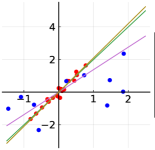
(a) $n_{1}=20,n_{2}=10$

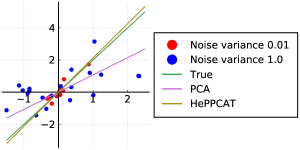
(b) $n_{1}=10,n_{2}=20$

Figure 1: Illustrative heteroscedastic examples with $k=1$ factor and $L=2$ noise variances $v_{1}=0.01$ and $v_{2}=1$. HePPCAT estimates variances to account for heteroscedasticity, recovering the true latent subspace much better than PCA.

3 Related works

3.1 Factor analysis and (homoscedastic) probabilistic PCA

In conventional factor analysis, samples in $d$ dimensions are modeled as follows:

$$\mathbf{y}_{i}=\mathbf{F}\mathbf{z}_{i}+\bm{\varepsilon}_{i},\quad i\in\{1,\dots,n\},$$

where $\mathbf{F}\in\mathbb{R}^{d\times k}$ contains the $k$ factors, $\mathbf{z}_{i}\overset{iid}{\sim}\mathcal{N}(\bm{0}_{k},\mathbf{I}_{k})$ are random coefficients, and $\bm{\varepsilon}_{i}\overset{iid}{\sim}\mathcal{N}(\bm{0}_{d},\bm{\Psi})$ are random noise with diagonal covariance $\bm{\Psi}$. The quantities $\mathbf{F},\mathbf{z}_{i},\bm{\varepsilon}_{i}$ and $\bm{\Psi}$ are all unknown. Marginalizing out $\mathbf{z}_{i}$ and $\bm{\varepsilon}_{i}$ yields a model where only $\mathbf{F}$ and $\bm{\Psi}$ are to be estimated by maximizing the marginal likelihood. In general, the column space of a maximum likelihood estimate for $\mathbf{F}$ will not coincide with the corresponding principal subspace of the data. Indeed, factor analysis and PCA are somewhat distinct approaches to dimensionality reduction; see, e.g., [6, Chapter 7].

However, maximum likelihood estimation does produce the principal subspace if the noise covariance is assumed to be isotropic, i.e., $\bm{\Psi}=v\,\mathbf{I}_{d}$ for some noise variance $v$. This model is the setting of probabilistic PCA [5]. In this case, the log-likelihood is

$$\mathcal{L}^{\mathrm{PPCA}}(\mathbf{F},v) \triangleq\frac{1}{2}\Big{[}n\ln\det(\mathbf{F}\mathbf{F}^{\prime}+v\mathbf{I})^{-1}-\operatorname{tr}\big{\{}\mathbf{Y}^{\prime}(\mathbf{F}\mathbf{F}^{\prime}+v\mathbf{I})^{-1}\mathbf{Y}\big{\}}\Big{]},$$

and is maximized by $\mathbf{F}=\mathbf{\widehat{U}}\operatorname{diag}^{1/2}(\hat{\lambda}_{1}-\bar{\lambda},\dots,\hat{\lambda}_{k}-\bar{\lambda})$ and $v=\bar{\lambda}$, where the columns of $\mathbf{\widehat{U}}\in\mathbb{R}^{d\times k}$ are principal eigenvectors of the sample covariance matrix $(\mathbf{y}_{1}\mathbf{y}_{1}^{\prime}+\cdots+\mathbf{y}_{n}\mathbf{y}_{n}^{\prime})/n$, $\hat{\lambda}_{1},\dots,\hat{\lambda}_{k}$ are the corresponding eigenvalues, and $\bar{\lambda}$ is the average of the remaining $d-k$ eigenvalues [7, 8, 5]. Moreover, [5, 9] characterize stationary points as well as the global maxima of the likelihood objective function. They also derive an efficient expectation maximization (EM) algorithm related to one derived for factor analysis [10], and illustrate how the approach naturally generalizes to similar models.

Here we develop a new probabilistic PCA method; unlike previous settings, the samples are no longer identically distributed. Noise variances are now heterogeneous, i.e., the noise is heteroscedastic across samples. The resulting likelihood is no longer maximized by scaled eigenvectors of the sample covariance, so new algorithms are needed. We developed an EM algorithm for estimating the factors given known noise variances in [4]; this paper extends that work by jointly estimating both the factors and the unknown noise variances.

3.2 Accounting for heteroscedastic noise via weighted PCA

A natural way to account for heteroscedastic noise is to use a weighted PCA [6, Section 14.2.1] that replaces the sample covariance with a weighted sample covariance. Namely, given weights $w_{1},\dots,w_{L}$, weighted PCA returns the leading eigenvectors $\mathbf{\hat{u}}_{1},\dots,\mathbf{\hat{u}}_{k}$ of $\sum_{\ell=1}^{L}w_{\ell}\mathbf{Y}_{\ell}\mathbf{Y}_{\ell}^{\prime}$. These eigenvectors solve the weighted optimization problem

$$\mathbf{\widehat{U}}\triangleq[\mathbf{\hat{u}}_{1},\dots,\mathbf{\hat{u}}_{k}]\in\operatorname*{argmax}_{\mathbf{U}\in\mathbb{R}^{d\times k}:\mathbf{U}^{\prime}\mathbf{U}=\mathbf{I}_{k}}\sum_{\ell=1}^{L}w_{\ell}\left\|\mathbf{U}^{\prime}\mathbf{Y}_{\ell}\right\|_{\mathrm{F}}^{2}.$$

A typical choice for the weights is inverse noise variance, i.e., $w_{\ell}=1/v_{\ell}$, so samples that are twice as noisy get half as much weight. Doing so effectively whitens the noise, is a type of maximum likelihood weighting [11], and can significantly improve performance [12]. However, as analyzed in [12], it can be better to more aggressively downweight noisier samples, especially for low signal-to-noise ratio (SNR) regimes. In particular, optimal weights for recovery of any individual component is between inverse noise variance and square inverse noise variance, which more aggressively downweights noisier samples. Weighted PCA with general weights does not have an obvious maximum likelihood formulation.

In contrast, this paper considers the maximum likelihood estimation of underlying factors and noise variances jointly. The resulting optimization problem does not appear to reduce to PCA with a weighted sample covariance, yielding a distinct approach to accounting for heteroscedasticity.

3.3 Heteroscedasticity across features

This paper focuses on noise that is heteroscedastic across samples, i.e., the samples are of varying quality. Noise can also be heteroscedastic across features. Indeed, much of the general literature on heteroscedasticity focuses on this manifestation. In the context of PCA, recent works have begun to study how to account for this form of heteroscedasticity. Notably, this heteroscedasticity induces a bias along the diagonal of the covariance matrix, causing conventional PCA to produce inaccurate components. To correct for this bias, [13] describes the HeteroPCA method that treats the diagonal entries as missing and iteratively imputes the values. Alternatively, [14, 15] combine whitening of the data with spectral shrinkages tailored to optimize, e.g., matrix denoising.

3.4 Accounting for heterogeneous clutter in RADAR

In the context of estimating low-rank clutter, [16, 17, 18] model $n$ independent samples $\mathbf{y}_{1},\dots,\mathbf{y}_{n}\in\mathbb{C}^{d}$ as

$$\mathbf{y}_{i}=\bm{\varepsilon}_{i}+\mathbf{c}_{i},\quad i\in\{1,\dots,n\},$$

where $\bm{\varepsilon}_{i}\overset{iid}{\sim}\mathcal{C}\mathcal{N}(\bm{0}_{d},\mathbf{I}_{d})$ is complex white Gaussian noise, and the clutter $\mathbf{c}_{i}\sim\mathcal{C}\mathcal{N}(\bm{0}_{d},\tau_{i}\bm{\Sigma})$ share a common rank-$k$ covariance $\bm{\Sigma}$ that is scaled by heterogeneous power factors $\tau_{i}$. Equivalently, $\mathbf{y}_{i}\sim\mathcal{C}\mathcal{N}(\bm{0}_{d},\tau_{i}\bm{\Sigma}+\mathbf{I}_{d})$ for $i\in\{1,\dots,n\}$. The goal is to estimate $\tau_{1},\dots,\tau_{n}$ and $\bm{\Sigma}$.

The low-rank covariance term $\tau_{i}\bm{\Sigma}$ is heterogeneous, while the noise is homogeneous. In contrast, the low-rank factor covariance in this paper is common among all the samples, and instead the noise is heterogeneous. The two models are related through an unknown heterogeneous rescaling because

$$\frac{1}{\sqrt{\tau_{i}}}\mathbf{y}_{i}\sim\mathcal{C}\mathcal{N}\{\bm{0}_{d},\bm{\Sigma}+(1/\tau_{i})\mathbf{I}_{d}\},\quad i\in\{1,\dots,n\},$$

has a common low-rank factor covariance $\bm{\Sigma}$ and heteroscedastic noise with variances $1/\tau_{1},\dots,1/\tau_{n}$. As a result, the two problems share some common challenges and approaches. Notably, the EM factor update (Section 5.1) is essentially the same (up to rescaling) as [18, Section III-B].

Nevertheless, the problems remain distinct due to the difference in how the unknown heterogeneity manifests. For example, heterogeneous power factors are only identifiable up to scale, since any change in scale can be absorbed by $\bm{\Sigma}$. The heterogeneous noise model we study does not have this scale ambiguity. Moreover, the likelihood for heterogeneous noise as a function of noise variances has a similar form as that for heterogeneous power factors, but with significant differences. Notably, decreasing a noise variance to zero sends the log-likelihood to $-\infty$ with unbounded curvature in the common case where the data are not perfectly fit. As a result, approaches well-designed for updating power factor estimates, such as the minorizer [18, Proposition 1], cannot always be directly applied to update the noise variance estimates. Different algorithms are needed.

In the context of heterogeneous power factors, [19] derives bounds on estimation performance and [20] places priors on the clutter subspace. These are also interesting directions for future work on heterogeneous noise.

3.5 Matrix Factorization

The model 1 that this paper focuses on can also be interpreted as a matrix factorization formulation that has Gaussian coefficients and additive noise. Within this framework there exist generalizations where one assumes other coefficient and noise distributions or even treats the factors or noise variances as random with a prior distribution. That is, one may generalize 1 to allow other distributions on $\mathbf{z}_{\ell,i},\bm{\varepsilon}_{\ell,i}$ and/or put a distribution on $\mathbf{F}$ or $v_{1},\dots,v_{L}$. There is a great deal of literature for factor analysis in a variety of settings, such as non-negative matrix factorization [21], Poisson matrix estimation [22], robust PCA [23], logistic PCA [24], and others [25, 26, 27, 28, 29]. Extending these models for heterogeneous noise is an interesting direction for future work.

In addition to this modeling work, great progress has been made in recent years to better understand why standard optimization algorithms perform well, even seeming to find the global minima/maxima, when applied to nonconvex matrix factorization problems [30, 31, 32, 33, 34, 35, 36, 37]. Three recent surveys summarize much of this progress [38, 39, 40] and thoroughly treat this related work. An overview of minorize maximize (MM) techniques and how they are applied to related problems can be found in [41]. Recent guarantees applied specifically to EM are found in [38]. None of the existing results apply directly to our setting for two reasons: first our model has noise that is not identically distributed across columns, and second we seek to optimize over both the factor matrix $\mathbf{F}$ and the additive noise variances $\mathbf{v}$ in our maximum likelihood formulation. If we consider only the problem of optimizing over the factor matrix, one could potentially extend results from [5, 32, 35] to characterize the stationary points of our objective.

Numerous works that involve matrix factorization use a spectral initialization, and several show that this initialization is sufficiently close to a good optima [30, 42]. We also use spectral initialization in our nonconvex optimization methods.

4 Expectation Maximization

A natural way to maximize the log-likelihood 2 is through an expectation maximization (EM) approach that produces a sequence of iterates $\mathbf{F}_{t}$ and $\mathbf{v}_{t}$ with non-decreasing log-likelihood. At each iteration, an EM method sets up a minorizer based on conditional expectation (E-step) that it then maximizes (M-step). This section derives an EM minorizer for the HePPCAT log-likelihood 2 at the iterates $\mathbf{F}_{t}$ and $\mathbf{v}_{t}$, where $t$ denotes iteration index. The resulting minorizer turns out to be challenging to maximize efficiently, so instead Section 5 proposes alternating algorithms, where some of the updates are based on the EM minorizer derived here.

Taking as complete data the samples $\mathbf{Y}_{1},\dots,\mathbf{Y}_{L}$ and (unknown) coefficients $\mathbf{Z}_{1},\dots,\mathbf{Z}_{L}$, where $\mathbf{Z}_{\ell}\triangleq[\mathbf{z}_{\ell,1},\dots,\mathbf{z}_{\ell,n_{\ell}}]\in\mathbb{R}^{k\times n_{\ell}}$ for $\ell\in\{1,\dots,L\}$, yields the following complete data log-likelihood

$$\mathcal{L}_{c}(\mathbf{F},\mathbf{v}) \triangleq\ln p(\mathbf{Y},\mathbf{Z};\mathbf{F},\mathbf{v})=\ln p(\mathbf{Y}|\mathbf{Z};\mathbf{F},\mathbf{v})+\ln p(\mathbf{Z};\mathbf{F},\mathbf{v})$$

$$=\sum_{\ell=1}^{L}\bigg{(}-\frac{dn_{\ell}}{2}\ln v_{\ell}-\frac{\left\|\mathbf{Y}_{\ell}-\mathbf{F}\mathbf{Z}_{\ell}\right\|_{\mathrm{F}}^{2}}{2v_{\ell}}-\frac{\left\|\mathbf{Z}_{\ell}\right\|_{\mathrm{F}}^{2}}{2}\bigg{)},$$ (5)

where 5 drops the constants $\ln(2\pi)^{-nd/2}$ and $\ln(2\pi)^{-nk/2}$.

For the E-step, take the expectation of 5 with respect to the conditionally independent distributions (from Bayes’ rule and the matrix inversion lemma):

$$\mathbf{z}_{\ell,i}|\mathbf{Y},\mathbf{F}_{t},\mathbf{v}_{t}\overset{\text{ind}}{\sim}\mathcal{N}(\mathbf{M}_{t,\ell}\mathbf{F}_{t}^{\prime}\mathbf{y}_{\ell,i},v_{t,\ell}\mathbf{M}_{t,\ell}),$$ (6)

where $\mathbf{M}_{t,\ell}\triangleq(\mathbf{F}_{t}^{\prime}\mathbf{F}_{t}+v_{t,\ell}\mathbf{I}_{k})^{-1}$, yielding minorizer

$$\mkern 3.0mu\overline{\mkern-3.0mu\mathcal{L}\mkern-1.0mu}\mkern 1.0mu(\mathbf{F},\mathbf{v};\mathbf{F}_{t},\mathbf{v}_{t})\triangleq\sum_{\ell=1}^{L}\bigg{[}-\frac{dn_{\ell}}{2}\ln v_{\ell}-\frac{\left\|\mathbf{Y}_{\ell}\right\|_{\mathrm{F}}^{2}}{2v_{\ell}}+\frac{1}{v_{\ell}}\operatorname{tr}(\mathbf{Y}_{\ell}^{\prime}\mathbf{F}\mathbf{\mkern 3.0mu\overline{\mkern-3.0muZ\mkern-1.0mu}\mkern 1.0mu}_{t,\ell})-\frac{1}{2v_{\ell}}\operatorname{tr}\{\mathbf{F}^{\prime}\mathbf{F}(\mathbf{\mkern 3.0mu\overline{\mkern-3.0muZ\mkern-1.0mu}\mkern 1.0mu}_{t,\ell}\mathbf{\mkern 3.0mu\overline{\mkern-3.0muZ\mkern-1.0mu}\mkern 1.0mu}_{t,\ell}^{\prime}+n_{\ell}v_{t,\ell}\mathbf{M}_{t,\ell})\}\bigg{]},$$ (7)

where $\mathbf{\mkern 3.0mu\overline{\mkern-3.0muZ\mkern-1.0mu}\mkern 1.0mu}_{t,\ell}\triangleq\mathbf{M}_{t,\ell}\mathbf{F}_{t}^{\prime}\mathbf{Y}_{\ell}\in\mathbb{R}^{k\times n_{\ell}}$ for $\ell\in\{1,\dots,L\}$, and 7 drops terms that are constant with respect to $\mathbf{F}$ and $\mathbf{v}$.

The corresponding M-step involves jointly maximizing 7 with respect to both $\mathbf{v}$ and $\mathbf{F}$, but doing so is challenging because the interaction of the variables remains complicated. See Appendix A for more discussion. However, optimization with respect to either (with the other fixed) is relatively easy, and Sections 5.1 and 5.2.2 use this minorizer to obtain efficient updates for the individual variables.

5 Alternating Algorithms

The challenge of jointly optimizing $\mathbf{F}$ and $\mathbf{v}$ using (2) or (7) motivates approaches that alternate between: a) optimizing $\mathbf{F}$ for fixed $\mathbf{v}$, and b) optimizing $\mathbf{v}$ for fixed $\mathbf{F}$. Namely, we consider a block-coordinate ascent of 2 with $\mathbf{F}$ and $\mathbf{v}$ as the two blocks of variables. These sub-problems are simpler but the sub-problem for updating $\mathbf{v}$ using (2) or (3) is still nontrivial so this section considers several methods for updating $\mathbf{v}$ given $\mathbf{F}$. When either the $\mathbf{F}$ or $\mathbf{v}$ update involves the conditional expectation with respect to some complete data, then such alternation is an instance of a space-alternating generalized EM (SAGE) algorithm [43].

5.1 Optimizing $\mathbf{F}$ for fixed $\mathbf{v}$ (via Expectation Maximization)

Fixing $\mathbf{v}$ at $\mathbf{v}_{t}$, maximizing the minorizer $\mkern 3.0mu\overline{\mkern-3.0mu\mathcal{L}\mkern-1.0mu}\mkern 1.0mu(\mathbf{F},\mathbf{v}_{t};\mathbf{F}_{t},\mathbf{v}_{t})$ in (7) with respect to $\mathbf{F}$ yields the EM step of [4]:

$$\mathbf{F}_{t+1}=\bigg{(}\sum_{\ell=1}^{L}\frac{\mathbf{Y}_{\ell}\mathbf{\mkern 3.0mu\overline{\mkern-3.0muZ\mkern-1.0mu}\mkern 1.0mu}_{t,\ell}^{\prime}}{v_{t,\ell}}\bigg{)}\bigg{(}\sum_{\ell=1}^{L}\frac{\mathbf{\mkern 3.0mu\overline{\mkern-3.0muZ\mkern-1.0mu}\mkern 1.0mu}_{t,\ell}\mathbf{\mkern 3.0mu\overline{\mkern-3.0muZ\mkern-1.0mu}\mkern 1.0mu}_{t,\ell}^{\prime}}{v_{t,\ell}}+n_{\ell}\mathbf{M}_{t,\ell}\bigg{)}^{-1},$$ (8)

that we compute via the SVD $\mathbf{F}_{t}=\mathbf{U}_{t}\bm{\Lambda}_{t}^{1/2}\mathbf{V}_{t}^{\prime}$:

$$\mathbf{F}_{t+1}=\bigg{(}\sum_{\ell=1}^{L}\frac{\mathbf{Y}_{\ell}\mathbf{\widetilde{Z}}_{t,\ell}^{\prime}}{v_{t,\ell}}\bigg{)}\bigg{(}\sum_{\ell=1}^{L}\frac{\mathbf{\widetilde{Z}}_{t,\ell}\mathbf{\widetilde{Z}}_{t,\ell}^{\prime}}{v_{t,\ell}}+n_{\ell}\mathbf{D}_{t,\ell}\bigg{)}^{-1}\mathbf{V}_{t}^{\prime},$$ (9)

where $\mathbf{\widetilde{Z}}_{t,\ell}\triangleq\mathbf{D}_{t,\ell}\bm{\Lambda}_{t}^{1/2}\mathbf{U}_{t}^{\prime}\mathbf{Y}_{\ell}$ and $\mathbf{D}_{t,\ell}\triangleq(\bm{\Lambda}_{t}+v_{t,\ell}\mathbf{I}_{k})^{-1}$ is easily inverted because $\bm{\Lambda}_{t}$ and $\mathbf{D}_{t,\ell}$ are diagonal. To show that this form is equivalent, note that $\mathbf{M}_{t,\ell}=\mathbf{V}_{t}\mathbf{D}_{t,\ell}\mathbf{V}_{t}^{\prime}$ and $\mathbf{\mkern 3.0mu\overline{\mkern-3.0muZ\mkern-1.0mu}\mkern 1.0mu}_{t,\ell}=\mathbf{V}_{t}\mathbf{\widetilde{Z}}_{t,\ell}$. See [4, Section 3] and [18, Section III-B] for similar derivations.

5.2 Optimizing $\mathbf{v}$ for fixed $\mathbf{F}$

Fixing $\mathbf{F}$ at $\mathbf{F}_{t}$, maximization of 3 with respect to $\mathbf{v}$ separates into $L$ univariate maximizations (over $v_{\ell}\geq 0$) of:

$$\mathcal{L}_{\ell}(v_{\ell})\triangleq-\sum_{j=0}^{k}\bigg{\{}\alpha_{j}\ln(\gamma_{j}+v_{\ell})+\frac{\beta_{j}}{\gamma_{j}+v_{\ell}}\bigg{\}},$$ (10)

where $\alpha_{0}\triangleq d-k$, $\beta_{0}\triangleq\left\|(\mathbf{I}_{d}-\mathbf{U}_{t}\mathbf{U}_{t}^{\prime})\mathbf{Y}_{\ell}\right\|_{\mathrm{F}}^{2}/n_{\ell}$, $\gamma_{0}\triangleq 0$,

$$j \geq 1: \alpha_{j} \triangleq 1, \beta_{j} \triangleq\|\mathbf{Y}_{\ell}^{\prime}\mathbf{u}_{t,j}\|_{2}^{2}/n_{\ell}, \gamma_{j} \triangleq\lambda_{t,j},$$

and $\mathbf{U}_{t}=[\mathbf{u}_{t,1},\dots,\mathbf{u}_{t,k}]$ and $\bm{\lambda}_{t}=(\lambda_{t,1},\dots,\lambda_{t,k})$ are the eigenvectors and eigenvalues of $\mathbf{F}_{t}\mathbf{F}_{t}^{\prime}$. Equation 10 drops all terms from 3 that are constant with respect to $v_{\ell}$ as well as a factor of $n_{\ell}/2$, and we define

$$\mathcal{L}_{\ell}(0)\triangleq\mathcal{L}_{\ell}(0^{+})=\begin{cases}+\infty,&\text{if }\beta_{t,\ell}\triangleq\sum_{j\in\mathcal{J}_{0}}\beta_{j}=0,\\ -\infty,&\text{otherwise},\end{cases}$$ (11)

where $\mathcal{J}_{0}\triangleq\{j\,:\,\gamma_{j}=0\}.$ Note also that $\mathcal{L}_{\ell}(+\infty)=-\infty$ and $\forall_{v_{\ell}\in(0,\infty)}\;\mathcal{L}_{\ell}(v_{\ell})<\infty$. Lacking an analytical solution for the critical points of (10) when $k>1$, we next describe several iterative methods for maximizing $\mathcal{L}_{\ell}(v_{\ell})$.

5.2.1 Global maximization via root-finding

If $\beta_{t,\ell}=0$, then 10 is maximized by $v_{\ell}=0$. Otherwise, $\mathcal{L}_{\ell}(0^{+})=-\infty$ and global maxima occur only at critical points. Differentiating 10 with respect to $v_{\ell}$ yields

$$\dot{}\mathcal{L}_{\ell}(v_{\ell})\triangleq\sum_{j=0}^{k}\bigg{\{}-\frac{\alpha_{j}}{\gamma_{j}+v_{\ell}}+\frac{\beta_{j}}{(\gamma_{j}+v_{\ell})^{2}}\bigg{\}}.$$ (12)

An upper bound for nonnegative roots of 12 can be obtained from general root bounds for polynomials, e.g., [44, 45]. We exploit the structure here to find a specialized bound. The $k+1$ summands in (12) are, respectively, positive to the left and negative to the right of $\beta_{j}/\alpha_{j}-\gamma_{j}$. As a result,

$$\dot{}\mathcal{L}_{\ell}(v_{\ell})>0 \text{ for }v_{\ell}<v_{\ell}^{\min}\triangleq\min_{j}(\beta_{j}/\alpha_{j}-\gamma_{j}),$$

$$\dot{}\mathcal{L}_{\ell}(v_{\ell})<0 \text{ for }v_{\ell}>v_{\ell}^{\max}\triangleq\max_{j}(\beta_{j}/\alpha_{j}-\gamma_{j}),$$

so all nonnegative critical points occur in $[v_{\ell}^{\min},v_{\ell}^{\max}]\cap[0,\infty)$ and can be found, e.g., via interval root-finding [46, Ch. 8]. Choosing the best among these critical points yields global maximizers.

This update maximally ascends the likelihood, and is perhaps the most natural choice. However, finding all the roots can be computationally expensive. Moreover, it is unclear whether fully maximizing the likelihood in this step is desirable since this update occurs within a broader alternating maximization. The current estimate of $\mathbf{F}$ may be far from optimal, so fully optimizing $\mathbf{v}$ might slow convergence. These reasons motivate alternative methods that we derive next.

5.2.2 Expectation Maximization

Although jointly updating $\mathbf{F}$ and $\mathbf{v}$ using 7 is challenging, it is fairly easy to update $\mathbf{v}$ when $\mathbf{F}$ is fixed. Replacing $\mathbf{F}$ in 7 with the current estimate $\mathbf{F}_{t}$ and simplifying leads to the following minorizer of (3) with respect to $v_{\ell}$:

$$\mkern 3.0mu\overline{\mkern-3.0mu\mathcal{L}\mkern-1.0mu}\mkern 1.0mu(\mathbf{F}_{t},\mathbf{v};\mathbf{F}_{t},\mathbf{v}_{t})=\sum_{\ell=1}^{L}\frac{n_{\ell}}{2}\bigg{(}-d\ln v_{\ell}-\frac{\rho_{t,\ell}}{v_{\ell}}\bigg{)},$$ (13)

where

$$\rho_{t,\ell} \triangleq\frac{1}{n_{\ell}}\big{[}\left\|\mathbf{Y}_{\ell}\right\|_{\mathrm{F}}^{2}-2\operatorname{tr}(\mathbf{Y}_{\ell}^{\prime}\mathbf{F}_{t}\mathbf{\mkern 3.0mu\overline{\mkern-3.0muZ\mkern-1.0mu}\mkern 1.0mu}_{t,\ell})+\operatorname{tr}\{\mathbf{F}_{t}^{\prime}\mathbf{F}_{t}(\mathbf{\mkern 3.0mu\overline{\mkern-3.0muZ\mkern-1.0mu}\mkern 1.0mu}_{t,\ell}\mathbf{\mkern 3.0mu\overline{\mkern-3.0muZ\mkern-1.0mu}\mkern 1.0mu}_{t,\ell}^{\prime}+n_{\ell}v_{t,\ell}\mathbf{M}_{t,\ell})\}\big{]}$$ (14)

$$=\left\|(\mathbf{I}_{d}-\mathbf{F}_{t}\mathbf{M}_{t,\ell}\mathbf{F}_{t}^{\prime})\mathbf{Y}_{\ell}\right\|_{\mathrm{F}}^{2}/n_{\ell}+v_{t,\ell}\operatorname{tr}(\mathbf{F}_{t}\mathbf{M}_{t,\ell}\mathbf{F}_{t}^{\prime}).$$

Maximizing 13 w.r.t. $v_{\ell}$ leads to the simple update:

$$v_{t+1,\ell}=\frac{\rho_{t,\ell}}{d}.$$ (15)

Since $\mathbf{F}_{t}\mathbf{M}_{t,\ell}\mathbf{F}_{t}^{\prime}=\mathbf{U}_{t}\bm{\Lambda}_{t}(\bm{\Lambda}_{t}+v_{t,\ell}\mathbf{I}_{k})^{-1}\mathbf{U}_{t}^{\prime}$, expanding and simplifying yields the following alternative formula for 14:

$$\rho_{t,\ell}=\sum_{j=0}^{k}\bigg{(}1-\frac{\gamma_{j}}{\gamma_{j}+v_{t,\ell}}\bigg{)}^{2}\beta_{j}+v_{t,\ell}\sum_{j=1}^{k}\frac{\lambda_{t,j}}{\lambda_{t,j}+v_{t,\ell}},$$ (16)

providing a more efficient form as well as a link to 10.

5.2.3 Difference of concave approach

The univariate objective 10 is a “difference of concave” or concave+convex cost function. One standard way to optimize such functions is to minorize each convex term with an affine function, leading to the following concave minorizer (ignoring constants):

$$\widetilde{\mathcal{L}}_{\ell}(v_{\ell};v_{t,\ell})\triangleq-\sum_{j=0}^{k}\bigg{\{}\frac{\alpha_{j}}{\gamma_{j}+v_{t,\ell}}v_{\ell}+\frac{\beta_{j}}{\gamma_{j}+v_{\ell}}\bigg{\}}.$$ (17)

Concavity of 17 eases maximization. If its derivative,

$$\dot{\widetilde{\mathcal{L}}}_{\ell}(v_{\ell};v_{t,\ell})\triangleq\sum_{j=0}^{k}\bigg{\{}-\frac{\alpha_{j}}{\gamma_{j}+v_{t,\ell}}+\frac{\beta_{j}}{(\gamma_{j}+v_{\ell})^{2}}\bigg{\}},$$

is nonpositive at the origin, i.e., $\dot{\widetilde{\mathcal{L}}}_{\ell}(0^{+};v_{t,\ell})\leq 0$, then 17 is maximized by $v_{\ell}=0$. Otherwise, at least one $\beta_{j}>0$ so 17 is necessarily strictly concave and is maximized at its unique critical point over $v_{\ell}>0$. This critical point can be efficiently computed, e.g., via bisection by noting that $\dot{\widetilde{\mathcal{L}}}_{\ell}(v_{\ell};v_{t,\ell})<0$ for $v_{\ell}>\max_{j}\{\sqrt{(\beta_{j}/\alpha_{j})(\gamma_{j}+v_{t,\ell})}-\gamma_{j}\}$.

5.2.4 Quadratic solvable minorizer

To derive a MM approach with a simple update, we separate the summation in (10) into the terms where $\gamma_{j}$ is zero and nonzero and apply the affine minorizer of (17) to the $\ln$ terms where $\gamma_{j}>0$ as follows:

$$\breve{\mathcal{L}}_{\ell}(v_{\ell};v_{t,\ell})= -\alpha_{t,\ell}\ln v_{\ell}-\frac{\beta_{t,\ell}}{v_{\ell}}-\zeta_{t,\ell}\,v_{\ell}-\sum_{j\notin\mathcal{J}_{0}}\frac{\beta_{j}}{\gamma_{j}+v_{\ell}},$$ (18)

where $\alpha_{t,\ell}\triangleq\sum_{j\in\mathcal{J}_{0}}\alpha_{j},$ $\zeta_{t,\ell}\triangleq\sum_{j\notin\mathcal{J}_{0}}\frac{\alpha_{j}}{\gamma_{j}+v_{t,\ell}},$ and $\beta_{t,\ell}$ was defined in (11).

For $j\notin\mathcal{J}_{0}$, let $\pi_{j}\triangleq\frac{\gamma_{j}}{\gamma_{j}+v_{t,\ell}}\in(0,1)$ and rewrite (18) as

$$\breve{\mathcal{L}}_{\ell}(v_{\ell};v_{t,\ell})=-\alpha_{t,\ell}\ln v_{\ell}-\frac{\beta_{t,\ell}}{v_{\ell}}-\zeta_{t,\ell}\,v_{\ell}-\sum_{j\notin\mathcal{J}_{0}}\frac{\beta_{j}}{\pi_{j}\left(\frac{\gamma_{j}}{\pi_{j}}\right)+(1-\pi_{j})\left(\frac{v_{\ell}}{1-\pi_{j}}\right)}$$

$$\geq \ \phi(v_{\ell};v_{t,\ell})\triangleq-\alpha_{t,\ell}\ln v_{\ell}-\frac{\beta_{t,\ell}}{v_{\ell}}-\zeta_{t,\ell}\,v_{\ell}-\sum_{j\notin\mathcal{J}_{0}}\beta_{j}\left(\pi_{j}\frac{1}{\gamma_{j}/\pi_{j}}+(1-\pi_{j})\frac{1}{v_{\ell}/(1-\pi_{j})}\right)$$

$$=-\alpha_{t,\ell}\ln v_{\ell}-\frac{B_{t,\ell}}{v_{\ell}}-\zeta_{t,\ell}v_{\ell},$$ (19)

using the concavity of the function $-1/x$, ignoring irrelevant constants, and defining

$$B_{t,\ell} =\beta_{t,\ell}+\sum_{j\notin\mathcal{J}_{0}}\beta_{j}\frac{v_{t,\ell}^{2}}{(\gamma_{j}+v_{t,\ell})^{2}}.$$

One can verify that, by design, $\phi(v_{t,\ell};v_{t,\ell})=\breve{\mathcal{L}}_{\ell}(v_{t,\ell};v_{t,\ell})$. The choice of $\pi_{j}$ originates from an EM algorithm for PET [43, 47]. Differentiating the concave minorizer $\phi$ yields:

$$0=-\frac{\alpha_{t,\ell}}{v_{\ell}}+\frac{B_{t,\ell}}{v_{\ell}^{2}}-\zeta_{t,\ell}.$$ (20)

This equation is solvable by the quadratic formula for $\zeta_{t,\ell}v_{\ell}^{2}+\alpha_{t,\ell}v_{\ell}-B_{t,\ell}$ that has exactly one positive root.

5.2.5 Cubic solvable minorizer

Because $\gamma_{j}>0$ in the final term of the concave minorizer in (18), that term has bounded curvature for $v_{\ell}\geq 0$, with maximum (absolute) curvature

$$c_{\ell,j}=-2\beta_{j}/\gamma_{j}^{3}.$$

Thus we have the following partially quadratic concave minorizer for (10) (ignoring constants):

$$Q_{l}(v_{\ell};v_{t,\ell})=-\alpha_{t,\ell}\ln v_{\ell}-\frac{\beta_{t,\ell}}{v_{\ell}}-\zeta_{t,\ell}\,v_{\ell}+\sum_{j\notin\mathcal{J}_{0}}\bigg{\{}\frac{\beta_{j}}{(\gamma_{j}+v_{t,\ell})^{2}}v_{\ell}+\frac{1}{2}c_{\ell,j}(v_{\ell}-v_{t,\ell})^{2}\bigg{\}}.$$ (21)

Differentiating and equating to zero yields

$$0 =\frac{-\alpha_{t,\ell}}{v_{\ell}}+\frac{\beta_{t,\ell}}{v_{\ell}^{2}}+\gamma_{t,\ell}+c_{t,\ell}\,(v_{\ell}-v_{t,\ell}),$$ (22)

$$\gamma_{t,\ell} \triangleq-\zeta_{t,\ell}+\sum\nolimits_{j\notin\mathcal{J}_{0}}\frac{\beta_{j}}{(\gamma_{j}+v_{t,\ell})^{2}},$$

$$c_{t,\ell} \triangleq\sum\nolimits_{j\notin\mathcal{J}_{0}}c_{\ell,j}.$$

This $v_{\ell}$ update corresponds to finding the appropriate root of a cubic polynomial. One could apply multiple $v_{\ell}$ updates based on (22). The fixed points of the resulting MM iteration are identical to the roots described by (12), so this approach is essentially an iterative root finding method with the nice MM property of monotonically increasing the log-likelihood.

5.3 Convergence and stopping criterion

All of the updates described above for $\mathbf{F}$ and $\mathbf{v}$ are based on minorizers, so like all block MM methods they provide updates that ensure the log-likelihood is monotonically non-decreasing. However, monotonicity alone is insufficient to ensure convergence when the individual updates may not have unique maximizers [48]. An alternative to simple alternation between the $\mathbf{F}$ and $\mathbf{v}$ blocks is the “maximum improvement” variant that calculates an update for both blocks and chooses the one that increases the likelihood the most [49]. This variant ensures convergence under modest regularity conditions (not requiring convexity or uniqueness) appropriate for the HePPCAT problem [50, Thm. 3]. To save computation, we used the simpler alternating maximization approach for the empirical results shown below.

A natural choice for stopping criterion is to stop once the change in the factor matrix is sufficiently small. Namely, iterate until $\left\|\mathbf{F}_{t+1}-\mathbf{F}_{t}\right\|_{\mathrm{F}}/\left\|\mathbf{F}_{t}\right\|_{\mathrm{F}}\leq\epsilon$, where $\epsilon\geq 0$ is a user-provided tolerance, as shown in Algorithm 1. That said, there are certainly other natural choices. For example, one could require sufficiently small changes in the noise variance estimates or in the log-likelihood.

5.4 Initialization by homoscedastic PPCA

Without prior knowledge of the noise variances, a natural choice to initialize $\mathbf{v}$ and $\mathbf{F}=\mathbf{U}\operatorname{diag}^{1/2}(\bm{\lambda})$ is the homoscedastic PPCA solution [5, Section 3.2]:

$$\mathbf{U}_{0} \triangleq\mathbf{\widehat{U}}, \bm{\lambda}_{0} \triangleq(\hat{\lambda}_{1}-\bar{\lambda},\dots,\hat{\lambda}_{k}-\bar{\lambda}), \mathbf{v}_{0} \triangleq\bar{\lambda}\bm{1}_{L},$$

where the $k$ columns of $\mathbf{\widehat{U}}\in\mathbb{R}^{d\times k}$ are principal eigenvectors of the sample covariance matrix $(\mathbf{Y}_{1}\mathbf{Y}_{1}^{\prime}+\cdots+\mathbf{Y}_{L}\mathbf{Y}_{L}^{\prime})/n$, $\hat{\lambda}_{1},\dots,\hat{\lambda}_{k}$ are the corresponding eigenvalues, and $\bar{\lambda}$ is the average of the remaining $d-k$ eigenvalues.

The HePPCAT optimization problem is nonconvex, so better maximizers might be found by taking the best among many random initializations, but we have not so far encountered such a case; see, e.g., the experiments in Section 10. The landscape of the objective appears to be favorable despite its nonconvexity. Moreover, initializing via homoscedastic PPCA provides a reasonable and nicely interpretable choice. If the samples are in fact close to homoscedastic, this initialization is likely close to optimal already. Even if not, it provides a homoscedastic baseline to improve upon via the alternating updates of Sections 5.1 and 5.2. All the updates are non-descending, so all iterates are guaranteed to have likelihood no worse than homoscedastic PPCA.

1

Input: Maximum number of iterations $T$, rank $k$, tolerance $\epsilon\geq 0$

Output: $\mathbf{F}\in\mathbb{R}^{d\times k}$, $\mathbf{v}\in\mathbb{R}_{+}^{L}$

Data: $[\mathbf{Y}_{1},\ldots,\mathbf{Y}_{L}]$, $\mathbf{Y}_{\ell}\in\mathbb{R}^{d\times n_{\ell}}\quad\ell=1,\ldots,L$

2 Initialize $\mathbf{F}_{0}$ and $\mathbf{v}_{0}$ via homoscedastic PPCA or random initialization

3 while iterations $t<T$ do

4       Update $\mathbf{F}_{t+1}$, fixing $\mathbf{v}$ at $\mathbf{v}_{t}$, using (9).

5       Update $\mathbf{v}_{t+1}$, fixing $\mathbf{F}$ at $\mathbf{F}_{t+1}$, using Root Finding or one step of one of the following updates:

• Expectation Maximization (16)

• Difference of concave minorizer (17)

• Quadratic solvable minorizer (20)

• Cubic solvable minorizer (22)

6      

7      if  $\left\|\mathbf{F}_{t+1}-\mathbf{F}_{t}\right\|_{\mathrm{F}}/\left\|\mathbf{F}_{t}\right\|_{\mathrm{F}}\leq\epsilon$  then

8             stop

9            

10       $t\leftarrow t+1$

11      

12

Algorithm 1 HePPCAT

6 Computational complexity

The primary sources of computational complexity in the EM update 8 for $\mathbf{F}$ are matrix multiplications and inverses. For each $\ell\in\{1,\dots,L\}$, computing $\mathbf{M}_{t,\ell}$ costs $O(k^{2}d+k^{3})$ after which computing $\mathbf{\mkern 3.0mu\overline{\mkern-3.0muZ\mkern-1.0mu}\mkern 1.0mu}_{t,\ell}$ costs $O(k^{2}d+kdn_{\ell})$, yielding a total cost of $O(Lk^{3}+Lk^{2}d+kdn)$. The remaining multiplications and inverses cost $O(kdn+k^{2}n+k^{2}d+k^{3})$. Combining these terms and noting that $k<d,n$ yields $O(Lk^{2}d+kdn)$. The alternative form 9 incurs an initial cost of $O(k^{2}d)$ to obtain the SVD of $\mathbf{F}_{t}$, but gains efficiency since $\mathbf{D}_{t,\ell}$ and $\mathbf{\widetilde{Z}}_{t,\ell}$ then cost $O(k)$ and $O(kdn_{\ell})$, respectively. As a result, this form has a final cost of $O(kdn)$ overall.

A leading order source of computational complexity for all of the $v_{\ell}$ update methods is in calculating the associated coefficients $\beta_{0},\dots,\beta_{k}$. Doing so incurs a cost of $O(kdn_{\ell})$ for each $\ell\in\{1,\dots,L\}$, yielding a cost of $O(kdn)$ overall. For all the $v_{\ell}$ updates (Sections 5.2.1, 5.2.2, 5.2.3, 5.2.4 and 5.2.5), the additional computational cost is independent of $d$ and $n$. Thus, one might suppose (since $k\ll d,n$ typically) that all the updates have essentially equal runtime. However, this is not the case. Global maximization (Section 5.2.1) and the difference of concave approach (Section 5.2.3) both use iterative algorithms for root-finding, and the runtime can depend significantly on not only $k$ but also properties of 10. Moreover, when $L$ is large, e.g., for block sizes of $n_{\ell}=1$, constant factors not captured by computational complexity can also have a significant impact. Section 7 compares the convergence speed of the various updates in practice, accounting for both their runtime costs and per-iteration improvement in likelihood.

To further improve computational efficiency, note that all the updates depend on $\mathbf{Y}_{\ell}$ implicitly through $\mathbf{Y}_{\ell}\mathbf{Y}_{\ell}^{\prime}$, so one could replace $\mathbf{Y}_{\ell}$ in the updates with any proxy $\mathbf{\breve{Y}}_{\ell}$ for which $\mathbf{\breve{Y}}_{\ell}\mathbf{\breve{Y}}_{\ell}^{\prime}=\mathbf{Y}_{\ell}\mathbf{Y}_{\ell}^{\prime}$. In some cases, e.g., when $n_{\ell}\gg d$, doing so can yield significant savings.

7 Comparison of update methods

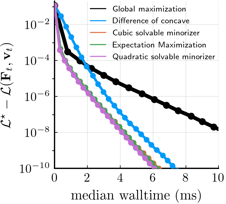
(a) Convergence w.r.t. $\mathcal{L}$.

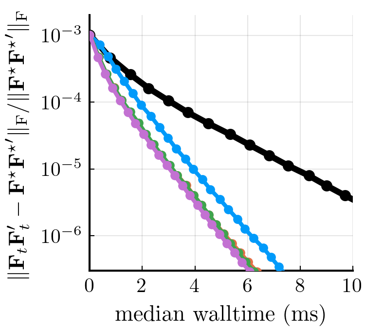
(b) Convergence w.r.t. $\mathbf{F}$.

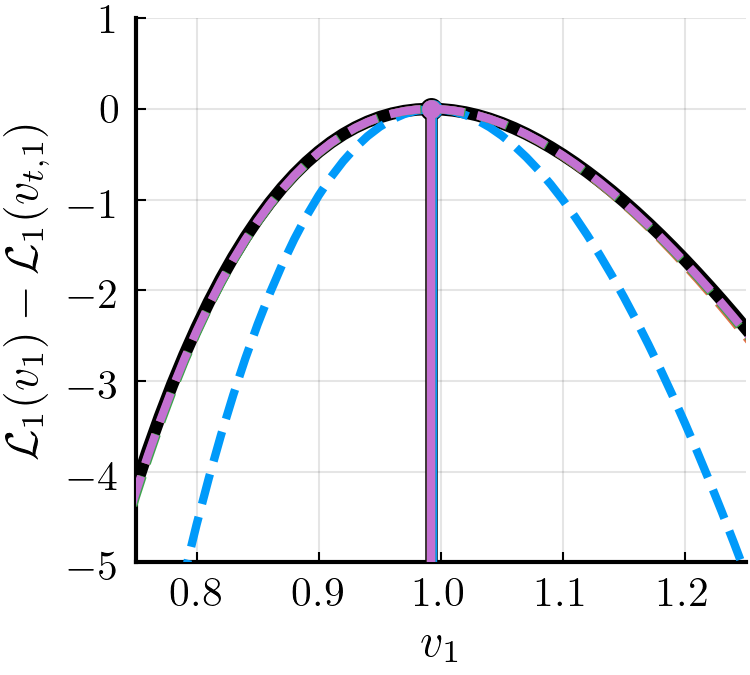
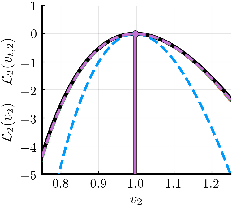
(c) Minorizers w.r.t. $\mathbf{v}$ at homoscedastic PPCA initialization.

Figure 2: Convergence of alternating maximization w.r.t. $\mathbf{F}$ and $\mathbf{v}$ for various $\mathbf{v}$ updates. We consider $n=10^{3}$ samples in $d=10^{2}$ dimensions with $k=3$ underlying factors $\bm{\tilde{\lambda}}=(4,2,1)$. The noise is homoscedastic: both the first $n_{1}=200$ and remaining $n_{2}=800$ samples have noise variance $\tilde{v}_{1}=\tilde{v}_{2}=1$. Walltimes are medians taken over 100 runs of the algorithm to reduce the effect of experimental noise. Markers denote each iteration.

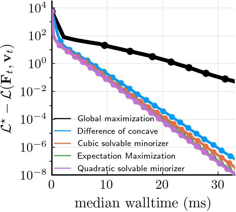
(a) Convergence w.r.t. $\mathcal{L}$.

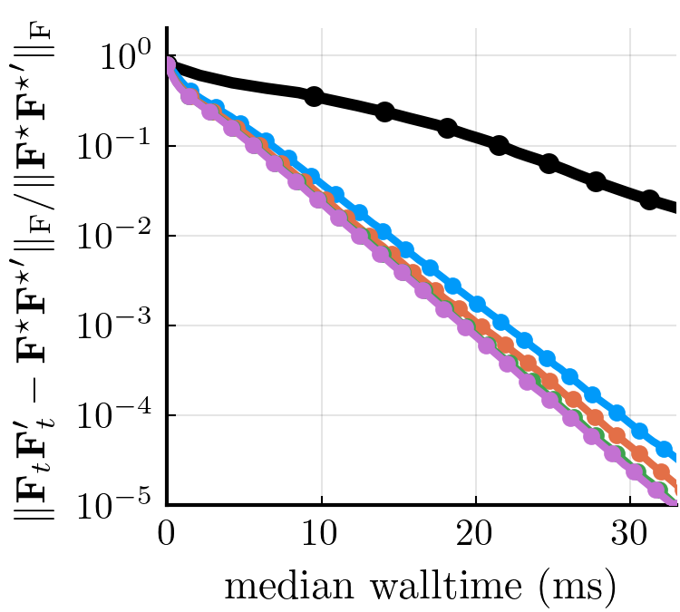
(b) Convergence w.r.t. $\mathbf{F}$.

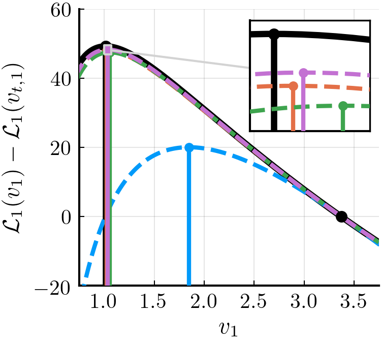
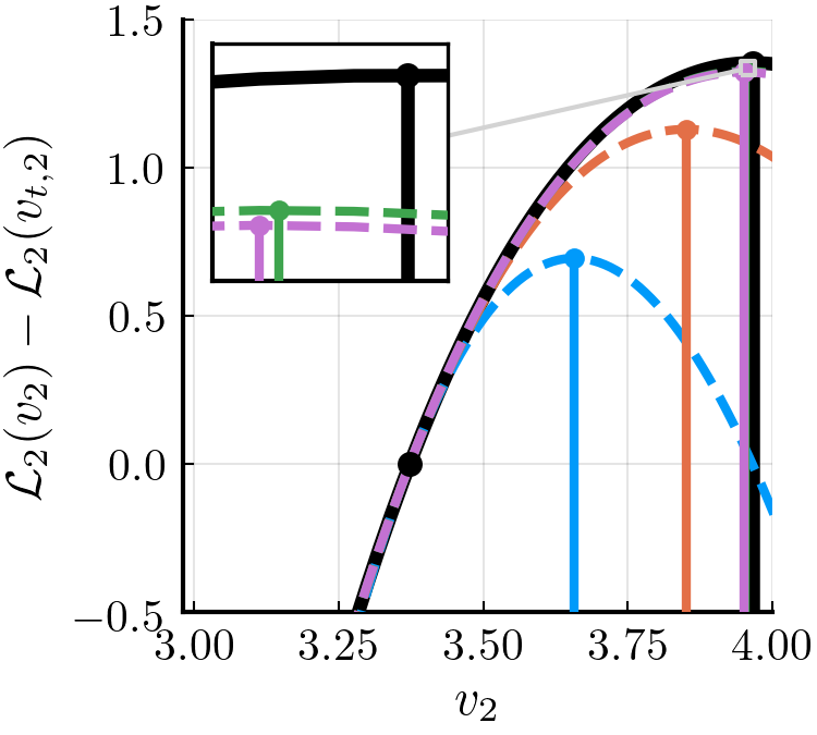
(c) Minorizers w.r.t. $\mathbf{v}$ at homoscedastic PPCA initialization.

Figure 3: Same as Fig. 2 except here the noise is heteroscedastic with $\tilde{v}_{2}=4$ and markers are placed every five iterations.

Section 5 described several update methods for $\mathbf{v}$ based on a variety of minorizers. It is not obvious a priori which choice is best, so this section compares their relative performance. We consider $n=10^{3}$ samples in $d=10^{2}$ dimensions generated according to the model 1 with $k=3$ factors generated as $\mathbf{\widetilde{F}}=\mathbf{\widetilde{U}}\operatorname{diag}^{1/2}(\bm{\tilde{\lambda}})$, where $\mathbf{\widetilde{U}}=(\mathbf{\tilde{u}}_{1},\dots,\mathbf{\tilde{u}}_{k})\in\mathbb{R}^{d\times k}$ is drawn uniformly at random from among $d\times k$ matrices having orthonormal columns and $\bm{\tilde{\lambda}}=(4,2,1)$. The first $n_{1}=200$ samples have noise variance $\tilde{v}_{1}=1$, and the remaining $n_{2}=800$ have noise variance $\tilde{v}_{2}$.

Fig. 2 considers the homoscedastic setting where $\tilde{v}_{2}=1$ (yet the two variances are still unknown to the algorithm). As a baseline, we take $\mathbf{F}^{\star}$ and $\mathbf{v}^{\star}$ to be the solutions obtained by 1000 iterations of Expectation Maximization updates for both $\mathbf{F}$ and $\mathbf{v}$. The associated log-likelihood is $\mathcal{L}^{\star}\triangleq\mathcal{L}(\mathbf{F}^{\star},\mathbf{v}^{\star})$. Fig. 2a plots convergence of the log-likelihood $\mathcal{L}^{\star}-\mathcal{L}(\mathbf{F}_{t},\mathbf{v}_{t})$ versus walltime for iterates $(\mathbf{F}_{t},\mathbf{v}_{t})$ obtained by the various choices for the $\mathbf{v}$ update. Note that $\mathcal{L}^{\star}-\mathcal{L}(\mathbf{F}_{t},\mathbf{v}_{t})$ is the log of the likelihood-ratio between the converged solution $(\mathbf{F}^{\star},\mathbf{v}^{\star})$ and iterate $(\mathbf{F}_{t},\mathbf{v}_{t})$. Fig. 2b plots convergence for the $\mathbf{F}$ iterates with respect to the normalized factor difference $\|\mathbf{F}_{t}\mathbf{F}_{t}^{\prime}-\mathbf{F}^{\star}{\mathbf{F}^{\star}}^{\prime}\|_{\mathrm{F}}/\|\mathbf{F}^{\star}{\mathbf{F}^{\star}}^{\prime}\|_{\mathrm{F}}$. Iterations are indicated on both plots by the markers, and walltime only includes the updates themselves (i.e., not calculation of the log-likelihood).

Among the $\mathbf{v}$ update methods, global maximization typically ascends the log-likelihood the most per iteration, but is also the most computationally expensive. As a result, it converges more slowly with respect to walltime. The difference of concave update is computationally cheaper but ascends the least per iteration initially. The final three updates (Cubic solvable MM, Expectation Maximization, Quadratic solvable MM) have fairly similar computational cost and log-likelihood increase per iteration.

The global maximization update corresponds to maximizing the univariate functions $\mathcal{L}_{\ell}(v_{\ell})$. The remaining update methods each correspond to maximizing an associated minorizer. Fig. 2c plots these minorizers at the homoscedastic PPCA initialization (Section 5.4), shifted to be zero at the current iterate. For this homoscedastic case, the homoscedastic PPCA initialization is already close to optimal and the minorizers (with the exception of the difference of concave minorizer) closely follow the log-likelihood.

Fig. 3 considers a heteroscedastic case with $\tilde{v}_{2}=4$. As in the homoscedastic case, global maximization converges the most slowly overall due to its high computational cost per iteration (more so in fact). Likewise, the difference of concave update is again computationally cheaper but ascends the least per iteration initially, and the remaining three update methods converge the most rapidly. Fig. 3c illustrates the comparative tightness of the various minorizers at the homoscedastic PPCA initialization. The initialization is far from optimal for this heteroscedastic case, and the relative differences in tightness among the minorizers are more clearly visible. Based on these experiments, we recommend using the EM minorizer or the quadratic solvable minorizer for the $\mathbf{v}$ updates.

8 Statistical performance experiments

This section evaluates the statistical performance of HePPCAT through simulation. We consider $n=10^{3}$ samples in $d=10^{2}$ dimensions generated according to the model 1 with $k=3$ factors generated as $\mathbf{\widetilde{F}}=\mathbf{\widetilde{U}}\operatorname{diag}^{1/2}(\bm{\tilde{\lambda}})$, where $\mathbf{\widetilde{U}}=[\mathbf{\tilde{u}}_{1},\dots,\mathbf{\tilde{u}}_{k}]\in\mathbb{R}^{d\times k}$ is drawn uniformly at random from among $d\times k$ matrices having orthonormal columns and $\bm{\tilde{\lambda}}=(4,2,1)$. The first $n_{1}=200$ samples have noise variance $\tilde{v}_{1}=1$, and the remaining $n_{2}=800$ have $\tilde{v}_{2}=\sigma_{2}^{2}$, where we sweep $\sigma_{2}$ from $0$ to $3$. We use $100$ iterations of alternating EM updates for $\mathbf{F}$ and $\mathbf{v}$ with the homoscedastic PPCA initialization.

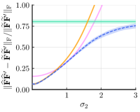
(a) Normalized factor estimation error

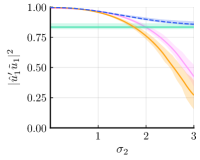
(b) Component 1 recovery

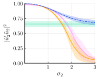
(c) Component 2 recovery

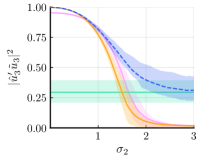
(d) Component 3 recovery

Figure 4: Comparison with homoscedastic PPCA applied on: i) full data, ii) only group 1, i.e, the $n_{1}=200$ samples with noise variance $\tilde{v}_{1}=1$, and iii) only group 2, i.e., the $n_{2}=800$ samples with noise variance $\tilde{v}_{2}=\sigma_{2}^{2}$. Lower is better in (a), and higher is better in (b)-(d). Heteroscedastic PPCA (HePPCAT) outperforms the homoscedastic methods on all four metrics. The mean and interquartile intervals (25th to 75th percentile) from $100$ data realizations are shown as curves and ribbons, respectively.

8.1 Comparison with homoscedastic methods

Fig. 4 compares the recovery of the latent factors $\mathbf{\widetilde{F}}$ by HePPCAT with those obtained by applying homoscedastic PPCA on: a) the full data, b) only group 1, i.e, the $n_{1}=200$ samples with noise variance $\tilde{v}_{1}=1$, and c) only group 2, i.e., the $n_{2}=800$ samples with noise variance $\tilde{v}_{2}=\sigma_{2}^{2}$. These homoscedastic PPCA approaches are reasonable and common choices in the absence of reliable heteroscedastic algorithms; it is worthwhile to understand their performance. The mean and interquartile intervals (25th to 75th percentile) from $100$ data realizations are shown as curves and ribbons, respectively.

Fig. 4a plots the normalized factor covariance estimation error, defined as $\|\mathbf{\widehat{F}}\mathbf{\widehat{F}}^{\prime}-\mathbf{\widetilde{F}}\mathbf{\widetilde{F}}^{\prime}\|_{\mathrm{F}}/\|\mathbf{\widetilde{F}}\mathbf{\widetilde{F}}^{\prime}\|_{\mathrm{F}}$ where $\mathbf{\widehat{F}}\in\mathbb{R}^{d\times k}$ is the estimated factor matrix. Figs. 4b, 4c and 4d plot the component recoveries $|\mathbf{\hat{u}}_{1}^{\prime}\mathbf{\tilde{u}}_{1}|^{2},\dots,|\mathbf{\hat{u}}_{3}^{\prime}\mathbf{\tilde{u}}_{3}|^{2}$, where $\mathbf{\hat{u}}_{1},\dots,\mathbf{\hat{u}}_{3}\in\mathbb{R}^{d}$ are the principal eigenvectors of $\mathbf{\widehat{F}}\mathbf{\widehat{F}}^{\prime}$. Lower is better for estimation error and higher is better for component recovery.

When $\sigma_{2}$ is small enough, homoscedastic PPCA applied to only group 2 performs the best among the homoscedastic PPCA’s. In this case, group 2 is relatively clean, and the components are reliably recovered. Using the full data incorporates more samples, but in this case including the noisier group 1 data does more harm than good since homoscedastic PPCA treats them uniformly. There is a tradeoff here between having more samples and including noisier samples. Finally, using only group 1 performs worst; it is smaller and noisier.

With increasing $\sigma_{2}$, the performance of homoscedastic PPCA degrades when applied to the full data or group 2 since they incorporate these increasingly noisy samples. The effect is more pronounced for using only group 2, and eventually the tradeoff reverses; using the full data becomes best among the homoscedastic PPCA options. In particular, when $\sigma_{2}=1$, the full data actually has homoscedastic noise and there is no statistical benefit to using only either group. As $\sigma_{2}$ continues to increase, group 2 data is eventually so noisy that it becomes best to only use group 1. Just past $\sigma_{2}>1$, however, using only group 1 remains worse than using only the noisier group 2 data. In this regime, the more abundant samples in group 2 win out over the cleaner samples in group 1. Which homoscedastic PPCA option performs best depends crucially on the interplay of these tradeoffs, making it unclear a priori which to use.

HePPCAT uses all the data but estimates and accounts for the heteroscedastic noise. In Fig. 4, it essentially matches or outperforms all three homoscedastic PPCA options across the entire range of $\sigma_{2}$. In particular, for small $\sigma_{2}$, it closely matches the performance of using only group 2, and for large $\sigma_{2}$ it closely matches that of using only group 1. In some sense, it appears to automatically ignore unreliable data. For moderate $\sigma_{2}$, it outperforms the three homoscedastic PPCA options. In this regime, it is suboptimal to ignore either group of data or to use both but treat them uniformly, and HePPCAT appropriately combines them.

Notably, HePPCAT performs nearly the same across this sweep as the variant developed in [4] that assumed known noise variances, even though the noise variances are now unknown and jointly estimated. See Fig. 14. Sections 8.3 and 8.4 study the quality of the noise variance estimates.

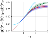
(a) Normalized subspace est. error

(b) Component 1 recovery

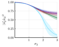
(c) Component 2 recovery

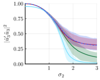
(d) Component 3 recovery

Figure 5: Comparison with heteroscedastic methods: HeteroPCA [13] and weighted PCA (inverse and square inverse noise variance weights calculated using the true noise variances). Lower is better in (a), and higher is better in (b)-(d). HePPCAT is among the best heteroscedastic methods. The mean and interquartile intervals (25th to 75th percentile) from $100$ data realizations are shown as curves and ribbons, respectively.

8.2 Comparison with heteroscedastic methods

Fig. 5 compares the recovery of the latent components $\mathbf{\widetilde{U}}$ by HePPCAT with those obtained by HeteroPCA [13] and by weighted PCA with: a) inverse noise variance weights, and b) square inverse noise variance weights. HeteroPCA is an iterative method designed for noise that is heteroscedastic within each sample; here we use $10$ iterations. Weighted PCA is a simple and efficient variant of PCA that accounts for heteroscedasticity across samples by down-weighting noisier samples. A typical choice for weights is inverse noise variance weighting that effectively rescales samples so their (scaled) noise becomes homoscedastic. Square inverse noise variance weighting is a choice of weights that more aggressively down-weights noisier samples. It can be more effective for weak signals, as revealed by the analysis in [12].

Fig. 5a plots the normalized subspace estimation error, defined as $\|\mathbf{\widehat{U}}\mathbf{\widehat{U}}^{\prime}-\mathbf{\widetilde{U}}\mathbf{\widetilde{U}}^{\prime}\|_{\mathrm{F}}/\|\mathbf{\widetilde{U}}\mathbf{\widetilde{U}}^{\prime}\|_{\mathrm{F}}$ where we denote the estimated factor eigenvectors as $\mathbf{\widehat{U}}=[\mathbf{\hat{u}}_{1},\dots,\mathbf{\hat{u}}_{k}]\in\mathbb{R}^{d\times k}$. Figs. 5b, 5c and 5d plot the corresponding component recoveries $|\mathbf{\hat{u}}_{1}^{\prime}\mathbf{\tilde{u}}_{1}|^{2},\dots,|\mathbf{\hat{u}}_{3}^{\prime}\mathbf{\tilde{u}}_{3}|^{2}$. As before, the mean and interquartile intervals (25th to 75th percentile) from $100$ data realizations are shown as curves and ribbons, respectively, and lower is better for estimation error and higher is better for component recovery.

When $\sigma_{2}$ is small, both weighted PCA methods perform similarly to HePPCAT. They both down-weight group 1 samples and benefit from the clean group 2 samples. As $\sigma_{2}$ increases, a gap in the performance appears between inverse noise variance and square inverse noise variance weighted PCA. In this regime, the more aggressive square inverse noise variance weights perform better for the weaker second and third components. For the stronger first component, inverse noise variance weights remain comparable and are, in fact, better for moderate $\sigma_{2}$. Throughout the sweep, HePPCAT matches or slightly outperforms the statistical performance of both weighted PCA methods. The relatively favorable performance of these methods highlights the benefit of accounting for heteroscedasticity across samples. Doing so enables them to make better use of all the available data. Note that unlike the two weighted PCA methods, HePPCAT is not given the noise variances and instead estimates them. Moreover, to apply the weighted PCA methods shown here, one must choose between the two weights (neither is uniformly better than the other), whereas HePPCAT works well across the range of noise variances.

HeteroPCA also accounts for heteroscedastic noise, but does so primarily for heteroscedasticity within each sample, rather than across samples. Heteroscedasticity within each sample biases the diagonal of the covariance matrix, even in expectation, and HeteroPCA corrects for this. However, it treats the samples themselves fairly uniformly. Consequently, its performance here closely resembles that of homoscedastic PPCA on the full data, as shown in Fig. 4. This behavior highlights the qualitative difference between heteroscedasticity within and heteroscedasticity across samples; they manifest differently and must both be addressed. Section 8.5 considers a setting with noise that is heteroscedastic in both ways and illustrates the opportunity for further works considering the combination.

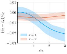
(a) Noise variance recovery

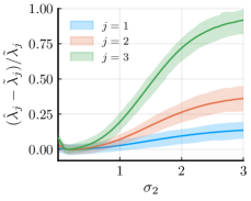
(b) Factor eigenvalue recovery

Figure 6: Relative bias of HePPCAT estimates for noise variances and factor eigenvalues. The mean and interquartile intervals (25th to 75th percentile) from $100$ data realizations are shown as curves and ribbons, respectively.

8.3 Bias in estimated noise variances and factor eigenvalues

Fig. 6 plots the relative biases of the estimated noise variances $\hat{v}_{1}$ and $\hat{v}_{2}$, as well as those of the estimated factor covariance eigenvalues $\bm{\hat{\lambda}}=(\hat{\lambda}_{1},\dots,\hat{\lambda}_{3})$. As before, the mean and interquartile intervals (25th to 75th percentile) from $100$ data realizations are shown as curves and ribbons, respectively, but now closer to zero is better. Positive values mean that HePPCAT has overestimated, and negative values indicate that it has underestimated. Taken together, Figs. 6a and 6b show a general negative bias in the estimated noise variances paired with a general positive bias in the estimated factor eigenvalues. This behavior is consistent with a corresponding behavior for homoscedastic PPCA in the setting of homoscedastic noise [52]. Providing a similar characterization for HePPCAT and a corresponding de-biasing procedure is an exciting, but nontrivial, direction for future work.

8.4 Dependence of noise variance estimates on block sizes

Fig. 7 fixes the noise variance of group 2 at $\tilde{v}_{2}=4$, i.e., $\sigma_{2}=2$, and shows the noise variances estimated for all of the $n=10^{3}$ samples when the samples are passed to HePPCAT in (non-overlapping) blocks of size 1, 10 and 100. Doing so reveals how the estimates depend on block size, and captures settings where the true latent groupings are unknown. Notably, a block size of 1 incorporates no a priori knowledge of the groupings. Fig. 7a shows a single representative data realization, and Fig. 7b shows the mean and interquartile intervals (25th to 75th percentile) obtained from $100$ data realizations. Both include corresponding histograms on the right showing the distributions of estimated noise variances.

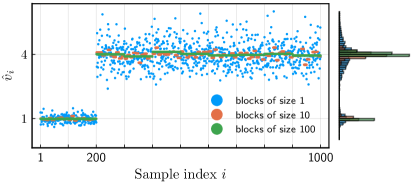
(a) Noise variance estimates for a single data realization.

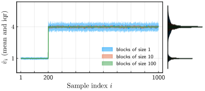
(b) Mean and interquartile intervals from $100$ data realizations.

Figure 7: Estimated noise variances for varying block sizes.

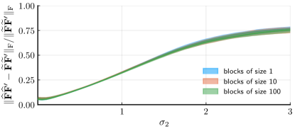
Figure 8: Normalized factor estimation error (median and interquartile intervals) for varying block sizes. The three block sizes have practically identical performance.

Notably, the estimates are fairly concentrated around the true latent noise variances of $\mathbf{\tilde{v}}=(1,4)$ at blocks of size $100$ even though this choice splits the first group of $n_{1}=200$ samples into two groups and the second group of $n_{2}=800$ into eight groups. These groups are visible in Fig. 7a as bars that tie together samples in the same block. Interestingly, blocks of size $10$ are not much more noisy, while being significantly less restrictive. Moreover, even using blocks of size $1$, at which point each sample is allowed its own noise variance estimate, provides relatively reliable estimates that cluster around the latent noise variances. The data contain enough information to obtain reasonable estimates of these noise variances. Nevertheless, when samples can be reasonably grouped together into blocks, e.g., grouping them by source or sensor, doing so can significantly denoise the estimates even when the blocks are relatively small. An interesting direction for future work is to jointly estimate these clusters from the data.

Fig. 8 plots the corresponding normalized factor estimation errors for $v_{2}=\sigma_{2}^{2}$ where $\sigma_{2}$ ranges from $0$ to $3$. The median and interquartile intervals (25th to 75th percentile) from $100$ data realizations are shown as curves and ribbons, respectively. We use the median here because the means for runs of block size 1, which are likely the most challenging, appeared to be skewed by outliers. Notably, all three block sizes perform quite closely to HePPCAT with known blocks and outperform homoscedastic variants (cf. Fig. 4a).

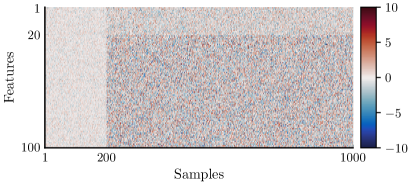
(a) Single data realization (heatmap).

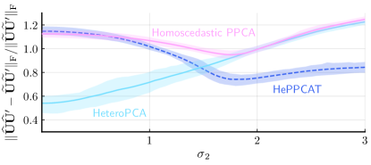
(b) Normalized subspace estimation error (lower is better).

Figure 9: Heteroscedasticity across both features and samples.

8.5 Additional heteroscedasticity within samples

Fig. 9 considers data that is heteroscedastic not just across samples, but also within samples. As before, the first group of $n_{1}=200$ samples have noise variance $v_{1}=1$, but now the second group of $n_{2}=800$ samples have a noise variance fixed at $v_{2}^{(1)}=4$ for the first $d^{(1)}=20$ features and noise variance $v_{2}^{(2)}=\sigma_{2}^{2}$ for the remaining $d^{(2)}=80$ features, where $\sigma_{2}$ ranges from $0$ to $3$. Noise in the first group is homoscedastic within each sample, but except for $\sigma_{2}=2$, noise in the second group is heteroscedastic within each sample. Fig. 9a shows an example data realization for $\sigma_{2}=3$; observe that the first group are uniformly noisy, the first 20 features of the second group are noisier, and the final 80 features are noisiest.

Fig. 9b plots the subspace estimation error across this range of heteroscedastic settings for homoscedastic PPCA; HePPCAT, which accounts for heteroscedasticity across samples; and HeteroPCA [13], which primarily accounts for heteroscedasticity within each sample. Namely, HeteroPCA accounts for bias in the diagonal of the covariance that is caused by within-sample heteroscedasticity, but treats the samples themselves uniformly. When $\sigma_{2}$ is small, accounting for heteroscedasticity within each sample is more important and HeteroPCA is better. However, the tradeoff reverses and HePPCAT becomes better as $\sigma_{2}$ grows towards $\sigma_{2}=2$, at which point samples are heteroscedastic only across samples. Interestingly, heteroscedasticity across samples appears to continue to dominate for $\sigma_{2}>2$. Homoscedastic PPCA is generally worst, as it does not account for either heteroscedasticity. HePPCAT performs similarly for small $\sigma_{2}$, where within-sample heteroscedasticity seems to dominate, and HeteroPCA is similar for large $\sigma_{2}$, where across-sample heteroscedasticity seems to dominate. These results highlight a qualitative difference between across-sample and within-sample heteroscedasticity; both must be addressed. Developing methods that simultaneously handle both types of heteroscedasticity, which outperform all three methods across this range, is an exciting direction for future work.

9 Real Data Experiments

This section applies HePPCAT to environmental monitoring data containing air quality measurements from both a few high precision instruments and a large network of low-cost consumer-grade sensors. High precision measurements are provided by the U.S. Environmental Protection Agency (EPA) and its partners. They maintain a nationwide network of Air Quality Index (AQI) sensor stations that measure, monitor, and distribute air quality data on the AirNow platform [53]. The recent proliferation of low-cost consumer-grade AQI sensors, such as PurpleAir [54], provides a second source of data. These sensors stream data continuously to developer platforms, such as ThingSpeak [55], creating a network of crowd-sourced air quality data with greater spatial coverage and resolution but generally lower precision.

We consider $\text{PM}_{2.5}$ particulate concentration readings (in $\mu g/m^{3}$) from the AirNow platform and from outdoor PurpleAir sensors across the central California region, i.e., within longitudes (-123.948, -119.246) and latitudes (35.853, 39.724), at the top of every hour from February 9-13, 2021. We chose 10 random PurpleAir sensors nearby each of 46 AirNow sensors to obtain balanced sensing coverage, and omitted hours where at least one of the AirNow sensors did not record a measurement. This gave $n_{1}=46$ AirNow samples $\mathbf{y}_{1,i}$ and $n_{2}=460$ PurpleAir samples $\mathbf{y}_{2,i}$, where each sample $\mathbf{y}_{\ell,i}$ is a vector of $d=108$ readings of $\text{PM}_{2.5}$ across time. Fig. 10 displays the map of the sensor locations for visualization. AirNow measurements are calibrated and averaged over hour-long windows by the U.S. EPA, whereas we collected the instantaneous readings from the PurpleAir sensors nearest to each hour. We centered the two sensor groups $\mathbf{Y}_{1}$ and $\mathbf{Y}_{2}$ separately by subtracting from each its sample mean.

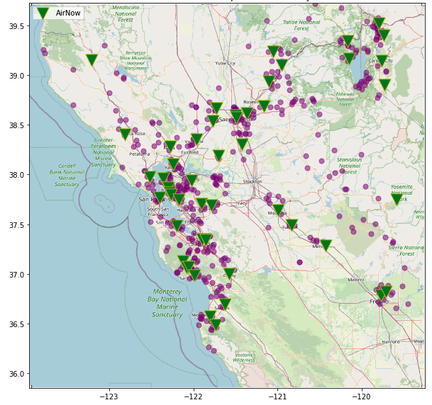
Figure 10: Sensor locations of AirNow (green triangles) and PurpleAir (purple circles) in the central California region of our experiments.

Lacking ground truth, we evaluate how well the subspace learned by HePPCAT on a subset of the samples generalizes to the rest. Namely, we randomly select $n^{\mathrm{(train)}}_{1}=25$ AirNow samples and $n^{\mathrm{(train)}}_{2}=250$ PurpleAir samples as training data $\mathbf{Y}^{\mathrm{(train)}}\in\mathbb{R}^{d\times n^{\mathrm{(train)}}}$. The remaining $n^{\mathrm{(test)}}_{1}=21$ AirNow samples and $n^{\mathrm{(test)}}_{2}=210$ PurpleAir samples serve as test data $\mathbf{Y}^{\mathrm{(test)}}\in\mathbb{R}^{d\times n^{\mathrm{(test)}}}$. The training data $\mathbf{Y}^{\mathrm{(train)}}$ is then used to estimate a basis for a $k=30$ dimensional subspace $\mathbf{\widehat{U}}\in\mathbb{R}^{d\times k}$ using PPCA and HePPCAT. We also consider PPCA-AN (PPCA on only the AirNow group $\mathbf{Y}^{\mathrm{(train)}}_{1}$) and PPCA-PA (PPCA on only the PurpleAir group $\mathbf{Y}^{\mathrm{(train)}}_{2}$). For each estimated $\mathbf{\widehat{U}}$, the performance on test data $\mathbf{Y}^{\mathrm{(test)}}$ is quantified by the normalized root mean-squared error (NRMSE) of the subspace reconstruction, i.e., $\|\mathbf{Y}^{\mathrm{(test)}}-\mathbf{\widehat{U}}\mathbf{\widehat{U}}^{\prime}\mathbf{Y}^{\mathrm{(test)}}\|_{\mathrm{F}}/\left\|\mathbf{Y}^{\mathrm{(test)}}\right\|_{\mathrm{F}}$. We also consider the corresponding NRMSE evaluated on only the AirNow test data $\mathbf{Y}^{\mathrm{(test)}}_{1}$ and on only the PurpleAir test data $\mathbf{Y}^{\mathrm{(test)}}_{2}$, as well as all the training data counterparts.

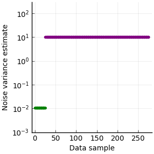
(a) A single representative trial.

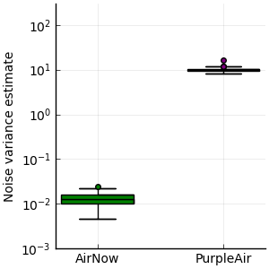
(b) Boxplots from all 200 trials.

Figure 11: Noise variance estimates from HePPCAT for a single representative trial LABEL:sub@fig:aqi_heppcat_variances:rep, and across all 200 trials LABEL:sub@fig:aqi_heppcat_variances:boxplot. In LABEL:sub@fig:aqi_heppcat_variances:rep, the first 25 samples in green are from AirNow, and the remaining purple samples are from PurpleAir. A single noise variance is estimated for each group. Boxplots in LABEL:sub@fig:aqi_heppcat_variances:boxplot show the spread of these estimates across the 200 trials. Units are in $(\mu g/m^{3})^{2}$.

We repeated this experiment for 200 random train-test splits of the data. Fig. 11a shows the noise variance estimates from HePPCAT from a representative trial. The estimated noise variance for the PurpleAir samples is substantially higher than that for AirNow samples, illustrating heterogeneity within this data. This is reasonable given that the PurpleAir data comes from low-cost consumer-grade sensors, while the AirNow data comes from high precision instruments. The corresponding box plots (indicating median, interquartile range, and outliers) in Fig. 11b show the spread of these estimates across the 200 trials. The estimates remain fairly consistent.

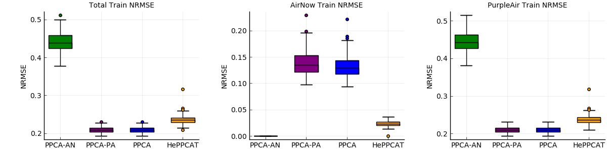
(a) NRMSE with respect to full training data $\mathbf{Y}^{\mathrm{(train)}}$, AirNow training data $\mathbf{Y}^{\mathrm{(train)}}_{1}$, and PurpleAir training data $\mathbf{Y}^{\mathrm{(train)}}_{2}$.

(b) NRMSE with respect to full test data $\mathbf{Y}^{\mathrm{(test)}}$, AirNow test data $\mathbf{Y}^{\mathrm{(test)}}_{1}$, and PurpleAir test data $\mathbf{Y}^{\mathrm{(test)}}_{2}$.

Figure 12: Air quality data were split into training and test sets. A $k=30$ dimensional subspace basis $\mathbf{\widehat{U}}$ was estimated from the training data using PPCA and HePPCAT, as well as PPCA-AN (PPCA trained using only the AirNow group) and PPCA-PA (PPCA trained using only the PurpleAir group). We evaluate the NRMSE $\|\mathbf{Y}-\mathbf{\widehat{U}}\mathbf{\widehat{U}}^{\prime}\mathbf{Y}\|_{\mathrm{F}}/\left\|\mathbf{Y}\right\|_{\mathrm{F}}$ with respect to both training and test data (as well as their AirNow and PurpleAir subsets). Lower is better for all plots. As expected, HePPCAT is never best on training data. However, it is among the best on all test cases, indicating that it has found explanatory components across both data sources.

Fig. 12 shows boxplots for the training and test NRMSEs across the 200 trials. As expected, PPCA (on full data) generally has the lowest training NRMSE on full data, PPCA-AN is generally best on AirNow training data, and likewise for PPCA-PA on PurpleAir training data. Compared with PPCA (on full data), HePPCAT has worse training NRMSE on the full data and on the PurpleAir data, but has better training NRMSE on the cleaner AirNow data. Turning to test NRMSE, however, HePPCAT is among the best with respect to not only AirNow data, but also the full data and even the PurpleAir data. HePPCAT appears to more effectively leverage information from both the cleaner but fewer AirNow samples and the noisier but more numerous PurpleAir samples.

Overall, the experiments here with air quality data illustrate heterogeneity arising naturally in real data and the potential for improved generalization by using HePPCAT.

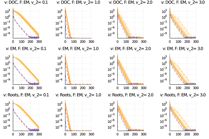
Figure 13: Convergence gaps of each algorithm to the maximum converged log-likelihood per heteroscedastic noise experiment. $n=[200,800]$ and $\mathbf{v}_{1}=1.0$.

10 Investigation of the landscape

This section empirically illustrates the favorable landscape of our optimization problem and our algorithms’ convergence to the globally optimal solution for synthetically generated data. Even though the nonconvexity of the problem might lead one to wonder if the choice of initialization matters, we find that does not appear to be the case. We generate the same low-rank heteroscedastic model as described in Section 8 and sweep across $\sigma_{2}^{2}$ values 0.1, 1.0, 2.0, and 3.0. The first regime should see HePPCAT largely down-weight group 1 and perform PCA on just group 2. At $\sigma_{2}^{2}=1$, the dataset is statistically homoscedastic, and we expect the landscape to behave similarly to that of PCA, which enjoys a well-known landscape that features no spurious local maxima and strict saddles [32]. As $\sigma_{2}^{2}$ increases, the distribution of the noise variances becomes more bimodal, and the PPCA solution deviates farther from the optimal log-likelihood value. In the low-noise end, the second data block has four times as many samples as the first block and a tenth of the noise variance. In the noisiest setting, the second data block has three times the noise variance.

For each noise setting, we record each algorithms’ log-likelihood at iteration $t$ and in Fig. 13 show the difference to the maximum log-likelihood found among all algorithms and trials. We run 100 trials of each HePPCAT algorithm with the initial estimate of $\mathbf{F}$ drawn randomly with i.i.d. Gaussian $\mathcal{N}(0,1)$ entries and the initial estimate of $\mathbf{v}$ drawn randomly with i.i.d. entries uniform on $[0,1)$. We also examine initializations from the homoscedastic PPCA solution and from the oracle planted model parameters. The converged likelihood values for each algorithm and choice of initialization concentrate tightly around the same maximum, with this behavior consistent across a wide range of heteroscedastic noise levels, indicating a well-behaved landscape.

In the homoscedastic regime, the results are consistent with our expectation that the PPCA initialization should be close to optimal, as shown in the second column of Fig. 13. We observe as the data noise variances become more imbalanced, the PPCA initialization becomes farther away from the global maximum, but is still orders of magnitude better in likelihood than random initialization. The oracle initialization has the best likelihood for all the heteroscedastic settings as expected, but is still suboptimal since we are maximizing a finite-sample likelihood. An interesting direction is to study how heteroscedastic noise affects the likelihood and its maximum in finite sample settings.

11 Conclusion

This paper developed efficient algorithms for jointly estimating latent factors and noise variances from data with heteroscedastic noise. Maximizing the likelihood is a nontrivial nonconvex optimization problem, and unlike the homoscedastic setting, it is seemingly unsolvable via singular value decomposition. The proposed algorithms alternate between updating the factor estimates and the noise variance estimates, with several choices for the noise variance update. It is unclear a priori which choice is best, and we compared their empirical convergence speeds in practice. Further numerical experiments studying the statistical performance highlighted the significant benefits of properly accounting for heteroscedasticity. Experiments on air quality data illustrated heterogeneity arising naturally in real data and improved generalization by using HePPCAT. Given the nonconvexity of the problem, one might wonder if initializing differently could lead to better maximizers. We provided empirical evidence that this is not the case; the landscape, while nonconvex, appears favorable.

Extensions of the approach to handle more general settings, e.g., missing data or additional heterogeneity across features, are interesting directions for further work. Likewise, there are many variations of PCA, e.g., nonnegative matrix factorization, and generalizations, e.g., unions of subspaces, that one could consider. An extension to consider kernel PCA would be interesting [56, 57], as noted by a reviewer. One might also incorporate a clustering step in the alternating algorithm to estimate not only the noise variances but also the blocks sharing a common noise variance. Alternatively, one could consider the $L$ groupings to be another latent variable in the log-likelihood, and attempt to jointly estimate them. Estimating the rank is another direction for further work. Many classical methods were designed for homoscedastic noise, and recent works, e.g., [14, 58, 59, 60], have begun to explore this problem under heteroscedastic settings. Some avenues for improving convergence speed are using momentum / extrapolation [61] of the alternating maximization updates, as well as incremental variants. One could also consider tackling the M-step in Section 4 via an inner block coordinate ascent with updates similar to those in Sections 5.1 and 5.2.2 that ascend the EM minorizer 7. This paper also raises several natural conjectures about the landscape of the nonconvex objective, which are beyond our present scope and are exciting areas for further theoretical analysis. Finally, it was observed in the homoscedastic setting that noise variance estimates tend to have a downward bias that can be characterized and accounted for [52]. A similar bias in variance estimates appears to occur in the heteroscedastic setting, and extending the previous approaches is a promising direction.

Appendix A Challenges in Expectation Maximization

To carry out Expectation Maximization via Section 4, one might attempt to maximize 7 with respect to both $\mathbf{v}$ and $\mathbf{F}$ by first completing the square:

$$\mkern 3.0mu\overline{\mkern-3.0mu\mathcal{L}\mkern-1.0mu}\mkern 1.0mu(\mathbf{F},\mathbf{v};\mathbf{F}_{t},\mathbf{v}_{t})=-\sum_{\ell=1}^{L}\bigg{(}\frac{dn_{\ell}}{2}\ln v_{\ell}+\frac{\left\|\mathbf{Y}_{\ell}\right\|_{\mathrm{F}}^{2}}{2v_{\ell}}\bigg{)}+\frac{1}{2}\operatorname{tr}\Big{\{}\mathbf{T}(\mathbf{v})\mathbf{S}(\mathbf{v})^{-1}\mathbf{T}(\mathbf{v})^{\prime}\Big{\}}-\frac{1}{2}\left\|\mathbf{F}\mathbf{S}(\mathbf{v})^{1/2}-\mathbf{T}(\mathbf{v})\mathbf{S}(\mathbf{v})^{-1/2}\right\|_{\mathrm{F}}^{2},$$

where the first two lines are constant with respect to $\mathbf{F}$, and

$$\mathbf{T}(\mathbf{v}) \triangleq\sum_{\ell=1}^{L}\frac{1}{v_{\ell}}\mathbf{Y}_{\ell}\mathbf{\mkern 3.0mu\overline{\mkern-3.0muZ\mkern-1.0mu}\mkern 1.0mu}_{t,\ell}^{\prime}, \mathbf{S}(\mathbf{v}) \triangleq\sum_{\ell=1}^{L}\frac{1}{v_{\ell}}(\mathbf{\mkern 3.0mu\overline{\mkern-3.0muZ\mkern-1.0mu}\mkern 1.0mu}_{t,\ell}\mathbf{\mkern 3.0mu\overline{\mkern-3.0muZ\mkern-1.0mu}\mkern 1.0mu}_{t,\ell}^{\prime}+n_{\ell}v_{t,\ell}\mathbf{M}_{t,\ell}).$$

Thus 7 is maximized with respect to $\mathbf{F}$ by $\mathbf{F}=\mathbf{T}(\mathbf{v})\mathbf{S}(\mathbf{v})^{-1}$, yielding the maximization problem with respect to $\mathbf{v}$ of

$$\mkern 3.0mu\overline{\mkern-3.0mu\mathcal{L}\mkern-1.0mu}\mkern 1.0mu(\mathbf{T}(\mathbf{v})\mathbf{S}(\mathbf{v})^{-1},\mathbf{v};\mathbf{F}_{t},\mathbf{v}_{t})=\frac{1}{2}\operatorname{tr}\Big{\{}\mathbf{T}(\mathbf{v})\mathbf{S}(\mathbf{v})^{-1}\mathbf{T}(\mathbf{v})^{\prime}\Big{\}}-\sum_{\ell=1}^{L}\bigg{(}\frac{dn_{\ell}}{2}\ln v_{\ell}+\frac{\left\|\mathbf{Y}_{\ell}\right\|_{\mathrm{F}}^{2}}{2v_{\ell}}\bigg{)}.$$ (23)

Equation 23 is not easily optimized with respect to $\mathbf{v}$ for $L>1$ because of the matrix product in the trace. This term introduces coupling among the noise variances $v_{\ell}$ that may keep the problem from separating into $L$ univariate problems. Intuitively, the noise variances $v_{\ell}$ appear to be coupled via their impact on the optimal latent factors $\mathbf{F}$. Novel approaches to efficiently optimize 23, e.g., by studying its critical points, is an interesting direction for future work.

Appendix B Comparison with known noise variances

Fig. 14 compares HePPCAT with the oracle variant developed in [4] that used known noise variances; the experimental setup matches that of Sections 8.1 and 8.2. Even though the noise variances are unknown and jointly estimated in HePPCAT, the performance is nearly the same.

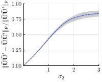
(a) Normalized subspace est. error

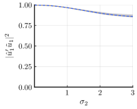
(b) Component 1 recovery

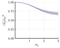
(c) Component 2 recovery

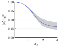
(d) Component 3 recovery

Figure 14: Comparison of the statistical performance of HePPCAT with the variant developed in [4] that assumed known noise variances, under the experimental sweep in Sections 8.1 and 8.2. Lower is better in (a), and higher is better in (b)-(d). HePPCAT performs nearly the same even though the noise variances are now unknown and jointly estimated.

References

- [1] D. Hong, L. Balzano, and J. A. Fessler, “Asymptotic performance of PCA for high-dimensional heteroscedastic data,” Journal of Multivariate Analysis, vol. 167, pp. 435–452, Sep. 2018.
- [2] R. N. Cochran and F. H. Horne, “Statistically weighted principal component analysis of rapid scanning wavelength kinetics experiments,” Analytical Chemistry, vol. 49, no. 6, pp. 846–853, May 1977.
- [3] O. Tamuz, T. Mazeh, and S. Zucker, “Correcting systematic effects in a large set of photometric light curves,” Monthly Notices of the Royal Astronomical Society, vol. 356, no. 4, pp. 1466–1470, Feb. 2005.
- [4] D. Hong, L. Balzano, and J. A. Fessler, “Probabilistic PCA for heteroscedastic data,” in 8th IEEE Intl. Workshop on Computational Advances in Multi-Sensor Adaptive Processing, 2019, pp. 26–30.
- [5] M. E. Tipping and C. M. Bishop, “Probabilistic Principal Component Analysis,” Journal of the Royal Statistical Society: Series B (Statistical Methodology), vol. 61, no. 3, pp. 611–622, Aug. 1999.
- [6] I. T. Jolliffe, Principal Component Analysis. Springer-Verlag, 2002.
- [7] D. Lawley, “A modified method of estimation in factor analysis and some large sample results,” in Uppsala symposium on psychological factor analysis, vol. 17, no. 19. Taylor & Francis, 1953, pp. 35–42.
- [8] T. W. Anderson and H. Rubin, “Statistical inference in factor analysis,” in Proceedings of the Third Berkeley Symposium on Mathematical Statistics and Probability, Volume 5: Contributions to Econometrics, Industrial Research, and Psychometry. University of California Press, 1956, pp. 111–150.
- [9] S. T. Roweis, “EM Algorithms for PCA and SPCA,” in Advances in Neural Information Processing Systems. MIT Press, 1998, pp. 626–632.
- [10] D. B. Rubin and D. T. Thayer, “EM algorithms for ML factor analysis,” Psychometrika, vol. 47, no. 1, pp. 69–76, Mar. 1982.
- [11] G. Young, “Maximum likelihood estimation and factor analysis,” Psychometrika, vol. 6, no. 1, pp. 49–53, Feb. 1941.
- [12] D. Hong, J. A. Fessler, and L. Balzano, “Optimally Weighted PCA for High-Dimensional Heteroscedastic Data,” 2018. [Online]. Available: http://arxiv.org/abs/1810.12862v2
- [13] A. Zhang, T. T. Cai, and Y. Wu, “Heteroskedastic PCA: Algorithm, optimality, and applications,” 2019. [Online]. Available: http://arxiv.org/abs/1810.08316v2
- [14] W. Leeb and E. Romanov, “Optimal spectral shrinkage and PCA with heteroscedastic noise,” 2020. [Online]. Available: http://arxiv.org/abs/1811.02201v4
- [15] W. Leeb, “Matrix denoising for weighted loss functions and heterogeneous signals,” 2020. [Online]. Available: http://arxiv.org/abs/1902.09474v3
- [16] A. Breloy, G. Ginolhac, F. Pascal, and P. Forster, “Clutter subspace estimation in low rank heterogeneous noise context,” IEEE Transactions on Signal Processing, vol. 63, no. 9, pp. 2173–2182, May 2015.
- [17] ——, “Robust covariance matrix estimation in heterogeneous low rank context,” IEEE Transactions on Signal Processing, vol. 64, no. 22, pp. 5794–5806, Nov. 2016.
- [18] Y. Sun, A. Breloy, P. Babu, D. P. Palomar, F. Pascal, and G. Ginolhac, “Low-complexity algorithms for low rank clutter parameters estimation in radar systems,” IEEE Transactions on Signal Processing, vol. 64, no. 8, pp. 1986–1998, Apr. 2016.
- [19] O. Besson, “Bounds for a mixture of low-rank compound-gaussian and white gaussian noises,” IEEE Transactions on Signal Processing, vol. 64, no. 21, pp. 5723–5732, Nov. 2016.
- [20] R. B. Abdallah, A. Breloy, M. N. E. Korso, and D. Lautru, “Bayesian signal subspace estimation with compound gaussian sources,” Signal Processing, vol. 167, p. 107310, Feb. 2020.
- [21] N. Gillis, “Introduction to nonnegative matrix factorization,” SIAM SIAG/OPT Views and News, vol. 25, no. 1, January 2017. [Online]. Available: http://wiki.siam.org/siag-op/images/siag-op/9/90/ViewsAndNews-25-1.pdf
- [22] Y. Cao and Y. Xie, “Poisson matrix recovery and completion,” IEEE Transactions on Signal Processing, vol. 64, no. 6, pp. 1609–1620, 2015.
- [23] G. Lerman and T. Maunu, “An overview of robust subspace recovery,” Proceedings of the IEEE, vol. 106, no. 8, pp. 1380–1410, 2018.
- [24] A. I. Schein, L. K. Saul, and L. H. Ungar, “A generalized linear model for principal component analysis of binary data,” in International Workshop on Artificial Intelligence and Statistics. PMLR, 2003, pp. 240–247.
- [25] D. J. Bartholomew, M. Knott, and I. Moustaki, Latent variable models and factor analysis: A unified approach. John Wiley & Sons, 2011, vol. 904.
- [26] M. Udell, C. Horn, R. Zadeh, and S. Boyd, “Generalized low rank models,” Foundations and Trends® in Machine Learning, vol. 9, no. 1, pp. 1–118, 2016.
- [27] J. Shi, X. Zheng, and W. Yang, “Survey on probabilistic models of low-rank matrix factorizations,” Entropy, vol. 19, no. 8, p. 424, 2017.
- [28] N. Vaswani, Y. Chi, and T. Bouwmans, “Rethinking PCA for modern data sets: Theory, algorithms, and applications [scanning the issue],” Proceedings of the IEEE, vol. 106, no. 8, pp. 1274–1276, 2018.
- [29] L. T. Liu, E. Dobriban, A. Singer et al., “PCA: high dimensional exponential family PCA,” Annals of Applied Statistics, vol. 12, no. 4, pp. 2121–2150, 2018.
- [30] Y. Chen, Y. Chi, J. Fan, C. Ma, and Y. Yan, “Noisy matrix completion: Understanding statistical guarantees for convex relaxation via nonconvex optimization,” SIAM Journal of Optimization, 2020.
- [31] L. Ding and Y. Chen, “Leave-one-out approach for matrix completion: Primal and dual analysis,” IEEE Transactions on Information Theory, 2020.
- [32] R. Ge, C. Jin, and Y. Zheng, “No spurious local minima in nonconvex low rank problems: A unified geometric analysis,” in Proceedings of the 34th International Conference on Machine Learning-Volume 70. JMLR, 2017, pp. 1233–1242.
- [33] R. Y. Zhang, S. Sojoudi, and J. Lavaei, “Sharp restricted isometry bounds for the inexistence of spurious local minima in nonconvex matrix recovery,” Journal of Machine Learning Research, vol. 20, no. 114, pp. 1–34, 2019.
- [34] R. Ge, J. D. Lee, and T. Ma, “Matrix completion has no spurious local minimum,” in Advances in Neural Information Processing Systems, 2016, pp. 2973–2981.
- [35] S. Bhojanapalli, B. Neyshabur, and N. Srebro, “Global optimality of local search for low rank matrix recovery,” in Advances in Neural Information Processing Systems, 2016, pp. 3873–3881.
- [36] J. Sun, “When are nonconvex optimization problems not scary?” Ph.D. dissertation, Columbia University, 2016.
- [37] D. Park, A. Kyrillidis, C. Carmanis, and S. Sanghavi, “Non-square matrix sensing without spurious local minima via the Burer-Monteiro approach,” in Artificial Intelligence and Statistics, 2017, pp. 65–74.
- [38] P. Jain and P. Kar, “Non-convex optimization for machine learning,” Foundations and Trends® in Machine Learning, vol. 10, no. 3-4, pp. 142–363, 2017.
- [39] Y. Chi, Y. M. Lu, and Y. Chen, “Nonconvex optimization meets low-rank matrix factorization: An overview,” IEEE Transactions on Signal Processing, vol. 67, no. 20, pp. 5239–5269, 2019.
- [40] Y. Zhang, Q. Qu, and J. Wright, “From symmetry to geometry: Tractable nonconvex problems,” 2020. [Online]. Available: http://arxiv.org/abs/2007.06753
- [41] Y. Sun, P. Babu, and D. P. Palomar, “Majorization-minimization algorithms in signal processing, communications, and machine learning,” IEEE Transactions on Signal Processing, vol. 65, no. 3, pp. 794–816, Feb. 2017.
- [42] Y. M. Lu and G. Li, “Phase transitions of spectral initialization for high-dimensional nonconvex estimation,” Information and Inference, to appear, 2019. [Online]. Available: http://arxiv.org/abs/1702.06435
- [43] J. A. Fessler and A. O. Hero, “Space-alternating generalized expectation-maximization algorithm,” IEEE Transactions on Signal Processing, vol. 42, no. 10, pp. 2664–2677, 1994.
- [44] M. Marden, Geometry of Polynomials. American Mathematical Society, Dec. 1949.
- [45] H. Hong, “Bounds for absolute positiveness of multivariate polynomials,” Journal of Symbolic Computation, vol. 25, no. 5, pp. 571–585, May 1998.
- [46] R. E. Moore, R. B. Kearfott, and M. J. Cloud, Introduction to Interval Analysis. Society for Industrial and Applied Mathematics, Jan. 2009.
- [47] A. R. De Pierro, “A modified expectation maximization algorithm for penalized likelihood estimation in emission tomography,” IEEE Trans. Med. Imag., vol. 14, no. 1, pp. 132–7, Mar. 1995.
- [48] M. J. D. Powell, “On search directions for minimization algorithms,” Mathematical Programming, vol. 4, no. 1, pp. 193–201, 1973.
- [49] B. Chen, S. He, Z. Li, and S. Zhang, “Maximum block improvement and polynomial optimization,” SIAM J. Optim., vol. 22, no. 1, pp. 87–107, 2012.
- [50] M. Razaviyayn, M. Hong, and Z. Luo, “A unified convergence analysis of block successive minimization methods for nonsmooth optimization,” SIAM J. Optim., vol. 23, no. 2, pp. 1126–53, 2013.
- [51] Y. Chikuse, Statistics on Special Manifolds. Springer New York, 2003.
- [52] D. Passemier, Z. Li, and J. Yao, “On estimation of the noise variance in high dimensional probabilistic principal component analysis,” Journal of the Royal Statistical Society: Series B (Statistical Methodology), vol. 79, no. 1, pp. 51–67, Dec. 2015.
- [53] U. E. P. Agency, “Air quality system data mart.” [Online]. Available: https://www.epa.gov/airdata
- [54] PurpleAir, “Real time air quality monitoring.” [Online]. Available: https://www2.purpleair.com
- [55] ThingSpeak. [Online]. Available: https://thingspeak.com
- [56] M. Tipping, “Sparse kernel principal component analysis,” in Neural Info. Proc. Sys., vol. 13, 2001. [Online]. Available: https://papers.nips.cc/paper/2000/hash/bf201d5407a6509fa536afc4b380577e-Abstract.html
- [57] N. Lawrence, “Probabilistic non-linear principal component analysis with Gaussian process latent variable models,” J. Mach. Learning Res., vol. 6, no. 60, pp. 1783–816, 2005. [Online]. Available: http://jmlr.org/papers/v6/lawrence05a.html
- [58] D. Hong, Y. Sheng, and E. Dobriban, “Selecting the number of components in PCA via random signflips,” 2020. [Online]. Available: http://arxiv.org/abs/2012.02985v1
- [59] Z. T. Ke, Y. Ma, and X. Lin, “Estimation of the number of spiked eigenvalues in a covariance matrix by bulk eigenvalue matching analysis,” 2020. [Online]. Available: http://arxiv.org/abs/2006.00436v1
- [60] B. Landa, T. T. C. K. Zhang, and Y. Kluger, “Biwhitening reveals the rank of a count matrix,” 2021. [Online]. Available: http://arxiv.org/abs/2103.13840v1
- [61] I. Y. Chun and J. A. Fessler, “Convolutional analysis operator learning: acceleration and convergence,” IEEE Trans. Im. Proc., vol. 29, no. 1, pp. 2108–22, Jan. 2020.