An Unsupervised Normalization Algorithm for Noisy Text: A Case Study for Information Retrieval and Stance Detection

Abstract

A large fraction of textual data available today contains various types of ‘noise’, such as OCR noise in digitized documents, noise due to informal writing style of users on microblogging sites, and so on. To enable tasks such as search/retrieval and classification over all the available data, we need robust algorithms for text normalization, i.e., for cleaning different kinds of noise in the text. There have been several efforts towards cleaning or normalizing noisy text; however, many of the existing text normalization methods are supervised, and require language-dependent resources or large amounts of training data that is difficult to obtain. We propose an unsupervised algorithm for text normalization that does not need any training data / human intervention. The proposed algorithm is applicable to text over different languages, and can handle both machine-generated and human-generated noise. Experiments over several standard datasets show that text normalization through the proposed algorithm enables better retrieval and stance detection, as compared to that using several baseline text normalization methods. Implementation of our algorithm can be found at https://github.com/ranarag/UnsupClean.

Keywords Data cleansing; unsupervised text normalization; morphological variants; retrieval; stance detection; microblogs; OCR noise

1 Introduction and Motivation

Digitization and the advent of Web 2.0 have resulted in a staggering increase in the amount of online textual data. As more and more textual data is generated online, or digitized from offline collections, the presence of noise in the text is a growing concern. Here noise refers to the incorrect forms of a valid word (of a given language). Such noise can be of two broad categories [1]: (1) machine-generated, such as those produced by Optical Character Recognition (OCR) systems, Automatic Speech Recognition (ASR) systems, etc. while digitizing content, and (2) human-generated, produced by the casual writing style of humans, typographical errors, etc. For instance, social media posts (e.g. microblogs) and SMS contain frequent use of non-standard abbreviations (e.g., ‘meds’ for ‘medicines’, ‘tmrw’ for ‘tomorrow’).

There exist plenty of important resources of textual data containing both the categories of noise. With regard to machine-generated noise, old documents like legal documents, defense documents, collections produced from large scale book digitization projects etc. are either in scanned version or in hard-copy format. Digitization of these vital collections involve OCR-ing the scanned versions. The print-quality, font variability, etc. lead to poor performance of the OCR systems which incorporates substantial error in the resulting text documents. Moreover, these noisy documents can be present in many languages, which also contributes to the challenge, since the OCR systems of many languages may not be well-developed. The unavailability of error-free versions of these collections makes error modelling infeasible.

For the second category of noise (user-generated), social networking sites such as Twitter and Weibo have emerged as effective resources for important real-time information in many situations [2, 3, 4]. Informal writing by users in such online media generates noise in the form of spelling variations, arbitrary shortening of words, etc. [5].

The presence of various types of noise are known to adversely affect Information Retrieval (IR), Natural Language Processing (NLP) and Machine Learning (ML) applications such as search/retrieval, classification, stance detection, and so on [6]. Hence, normalization/cleansing of such noisy text has a significant role in improving performance of downstream NLP / IR / ML tasks. The soul of a text normalization technique lies in mapping the different variations of a word to a single ‘normal’ form, achieving which successfully can lead to remarkable improvement in a lot of downstream tasks. There have been several works that have attempted text normalization, both in supervised and unsupervised ways (see Section 2 for a survey). Supervised algorithms require large training data (e.g., parallel corpora of noisy and clean text) which is expensive to obtain. This leads to a necessity for unsupervised methods, on which we focus in this paper.

There already exist several unsupervised text normalization approaches. However, most of the existing works have experimented with only one type of noise. For instance, Ghosh et al. [7] developed a method for correcting OCR errors, while others [8, 9] addressed variations in tweets. The type of errors in various text collections can be quite different – usually in tweets the error does not occur at the beginning of a word. However, OCR errors can appear at any location in a word, which makes noisy text normalization more challenging. So, a robust text normalization system for generic noise should be adept at handling many random and unseen error patterns. But to our knowledge, no one has attempted to address different categories of noise at the same time.

In this paper, we propose a novel unsupervised, language-independent algorithm – called UnsupClean – capable of automatically identifying the noisy variants produced by any of the aforementioned categories of noise, viz. machine-generated and human-generated.

We perform extensive experiments where we compare the proposed UnsupClean algorithm with four baseline text normalization algorithms – Aspell, Enelvo [9], and the algorithms developed by Sridhar et al [8] and Ghosh et al. [7]. To compare the performance of the various text normalization algorithms, we focus on two practical downstream applications – retrieval/search, and stance detection. We judge the performance on a text normalization algorithm by checking the performance of state-of-the-art retrieval/stance detection models on datasets cleaned by the normalization algorithm. Experiments are performed over several standard datasets spanning over two languages (English and Bengali), both containing OCR noise, as well as over microblogs containing human-generated noise. The empirical evaluation demonstrates the efficacy of our proposed algorithm over the baseline normalization algorithms – while we produce significantly better performance on OCR collections, our performance is competitive with all the baselines over the microblog collections. To our knowledge, no prior work on text normalization/cleansing have reported such detailed comparative evaluation as done in this work – over two downstream applications, and over six datasets spanning two languages and both machine-generated and user-generated noise.

To summarize, the strengths of the proposed text normalization algorithm UnsupClean are as follows: (1) The algorithm is completely unsupervised, and does not need any training data (parallel corpus), dictionaries, etc. Thus, the algorithm is suitable for application on resource-poor languages. (2) The algorithm can handle different types of noise, including both intentional mis-spellings by human users, as well as machine-generated noise such as OCR noise, and (3) The algorithm is language-independent, and can be readily applied to text in different languages. We make the implementation of UnsupClean publicly available at https://github.com/ranarag/UnsupClean.

The remainder of the paper is organized as follows. Section 2 briefly surveys various types of text normalization/cleaning algorithms. The proposed text normalization algorithm (UnsupClean) is detailed in Section 3. The baseline text normalization algorithms with which the performance of UnsupClean is compared, are described in Section 4. Next, to check the effectiveness of various text normalization algorithms, we focus on two downstream applications over noisy text – retrieval and stance detection. The experiments related to these two downstream applications are described in Section 5 and Section 6 respectively. Each of these sections describe the datasets used, the retrieval / stance detection models used, and the experimental results. Finally, we conclude the study in Section 7.

2 Related work

Textual content can contain different types of noise [1], and significant amount of research has been done on noisy text. Some prior works attempted to understand the effect of noise present in text data on applications such as classification [6]. Also some works have explored the use of artificially generated noise for cleansing noisy text. For instance, Gadde et al. [10] proposed methods for artificially injecting noise in text, through random character deletion, replacement, phonetic substitution, simulating typing errors, and so on.

Several methods have been developed for the normalization of noisy text, especially microblogs [11, 12, 13]. Based on the approach taken, text normalization methods can be broadly classified into two categories:

Supervised text normalization methods: Such approaches rely on a training dataset, which is usually a parallel corpus of canonical (correct) and noisy strings. For example, in [14], a noisy channel model was employed to perform text normalization. Incorporation of phonetic information has been shown to help text normalization, e.g., Toutanova et. al [15] included word pronunciation information in a noisy channel framework. GNU Aspell (http://aspell.net/), a popular spelling correction tool, also uses phonetic and lexical information to find normalized words.

More recently, neural models such as RNN [16] and Encoder-Decoder models [17] have also been used for text normalization. Some prior works have also modeled the text normalization problem as machine translation from the noisy text to the clean version [18].

Supervised methods require huge amounts of training data in the form of a parallel corpus, i.e., pairs of noisy and clean text. Such a parallel corpus is often difficult to get, especially for low-resource languages. Even for resource-rich languages, creating a training dataset involves a lot of human intervention, thus making it a costly process. Unsupervised methods try to mitigate some of these problems.

Unsupervised text normalization methods: These methods make use of the contextual and lexical information available from the corpora to perform normalization, without the need for any training data. For instance, Kolak et al. [19] applied a noisy channel based pattern recognition approach to perform OCR text correction. Ghosh et al. [7] used a combination of contextual and syntactic information to find the morphological variants of a word. Word embeddings (e.g., Word2vec [20]) have shown great potential in capturing the contextual information of a word, and hence word embedding based contextual information has been used in many of the recent works [8, 9]. For instance, Sridhar [8] used contextual information to find a set of candidate variants, which is refined based on a lexical similarity score.

In this work, we propose an unsupervised text normalization algorithm, and show that it performs competitively with some of the methods mentioned above [8, 7].

Task-independent vs. Task-specific text normalization methods: Text normalization methods can also be categorized into two broad categories based on whether a method is meant for a specific task. Most of the methods stated above, including spelling correction tools, are task-independent – they aim to correct the misspelled words in a corpus. On the other hand, some task-specific text normalization methods have also been proposed. For instance, Satapathy et al. [21] proposed a method for normalizing tweets specifically for sentiment analysis. Vinciarelli et al. [6] attempted normalization of noisy text specifically for categorization. Again, Ghosh et al. [7] used co-occurrence counts and edit-distance measures to find morphological variants of query words for the task of information retrieval from OCR-ed documents.

The proposed method is a task-independent one, and the experiments in the paper show that the data cleansing performed by the proposed method can be helpful for various tasks such as retrieval and stance detection.

3 Proposed Text Normalization Algorithm

This section describes the proposed unsupervised text normalization algorithm, which we call UnsupClean. The implementation is publicly available at https://github.com/ranarag/UnsupClean. We start this section with an overview of our proposed algorithm, and then describe every step in detail.

3.1 Overview of our algorithm

We look at text normalization from the perspective of identifying morphological variations of words. To understand this objective, we first need to understand what a morpheme is. According to Morphology (the area of linguistics concerned with the internal structure of words), a morpheme is the smallest unit of a word with a meaning. Structural variations to a morpheme or a combination of morphemes are known as morphological variations. There can be various types of morphological variations, including the plural and possessive forms of nouns, the past tense, past participle and progressive forms of verbs, and so on. Our approach attempts to identify such (and other) morphological variants of words (which are combinations of morphemes).

Intuitively, most morphological variations of a word have high string similarity with the canonical form of the word. So a string similarity based approach can be used to find candidate morphological variants of a word. However, string similarities can be misleading, e.g., the words ‘Kashmiri’ and ‘Kashmira’ have high string similarity, but one is an adjective (meaning ‘belonging to the state of Kashmir, India’) while the other is the name of an Indian actress. In such cases, it is useful to check the contextual similarity of the words.

An important question is how to measure contextual similarity between words. One potential way is to check co-occurrence counts of the words, i.e., how frequently the words appear in the same document (same context). However, for short-length documents (e.g., microblogs), the co-occurrence counts will mostly be zero (or very low), since two variants of the same word would usually not occur in the same microblog. An alternative method is to utilize word embeddings that capture contextual features of a word (e.g., Word2vec [20]). Hence, our algorithm uses a mixture of string similarity, word co-occurrence counts, and embeddings to find the morphological variants of words.

Symbol	Description	Symbol	Description
$C$	Corpus of documents which needs to be cleaned
$L$	Lexicon of noisy words	$L_{c}$	Lexicon of clean words
$w_{L}$	Noisy word	$w_{L_{c}}$	Clean word
$Cl_{w_{L_{c}}}$	cluster of morphological variants of word $w_{L_{c}}$	$CL$	set of clusters
$BLCS(w_{1},w_{2})$	Bi-character Longest Common Subsequence between $w_{1}$ and $w_{2}$	$LCSR(w_{1},w_{2})$	Longest Common Subsequence Ratio between words $w_{1}$ and $w_{2}$
$BLCSR(w_{1},w_{2})$	$BLCS$ Ratio between $w_{1}$ and $w_{2}$	$\alpha$	Threshold used to form cluster of words having $BLCSR$
$ES(w_{1},w_{2})$	Edit Similarity between words $w_{1}$ and $w_{2}$	$A(w_{L_{c}})$	cluster of words having lexical similarity with $w_{L_{c}}$ > $\alpha$
$G(w)$	Graph of words as nodes and edges weighted with the contextual similarity amongst them	$\beta$	a threshold used to prune the graph $G$
$\gamma$	threshold used in Ghosh et. al. [7]	$n$	threshold used in Enelvo [9]

Table 1: Notations used in this paper.

Table 1 lists the notations used in this paper. Our proposed model considers as input a corpus $C$ of noisy documents (that need to be cleaned). Let $L$ be the set of all distinct words contained in all the documents in $C$. Let $L_{c}$ be a lexicon of words with correct spellings, and let $w_{L_{c}}\in L_{c}$ be a correct word. For each word $w_{L_{c}}\in L_{c}$, our model finds a set $Cl_{w_{L_{c}}}$ of morphological variants of $w_{L_{c}}$, where every element of $Cl_{w_{L_{c}}}$ is a term in $L$. To find the set $Cl_{w_{L_{c}}}$ of morphological variants of $w_{L_{c}}$, our model employs the following four steps: (1) First, we use structural/lexical similarity measures to generate a set of candidate morphological variants for $w_{L_{c}}$. (2) Then we construct a similarity graph of the morphological variants, based on the similarity between word embeddings and co-occurrence counts of words. (3) We fragment the graph into clusters of similar morphological variants, using a graph clustering algorithm [22]. This step forms cluster of words which have both high semantic similarity as well as syntactic similarity with $w_{L_{c}}$. (4) Lastly, we choose that cluster of morphological variants as $Cl_{w_{L_{c}}}$, which has the member with the highest structural similarity with $w_{L_{c}}$. We then, club $Cl_{w_{j}}$ to $Cl_{w_{L_{c}}}$ for all $w_{j}\in Cl_{w_{j}}$ belonging to $Cl_{w_{L_{c}}}$. Subsequently, all words in $Cl_{w_{L_{c}}}$ are replaced by $w_{L_{c}}$. This results in non-overlapping clusters of morphological variants. Finally, all words belonging to a particular cluster are replaced by the same word.

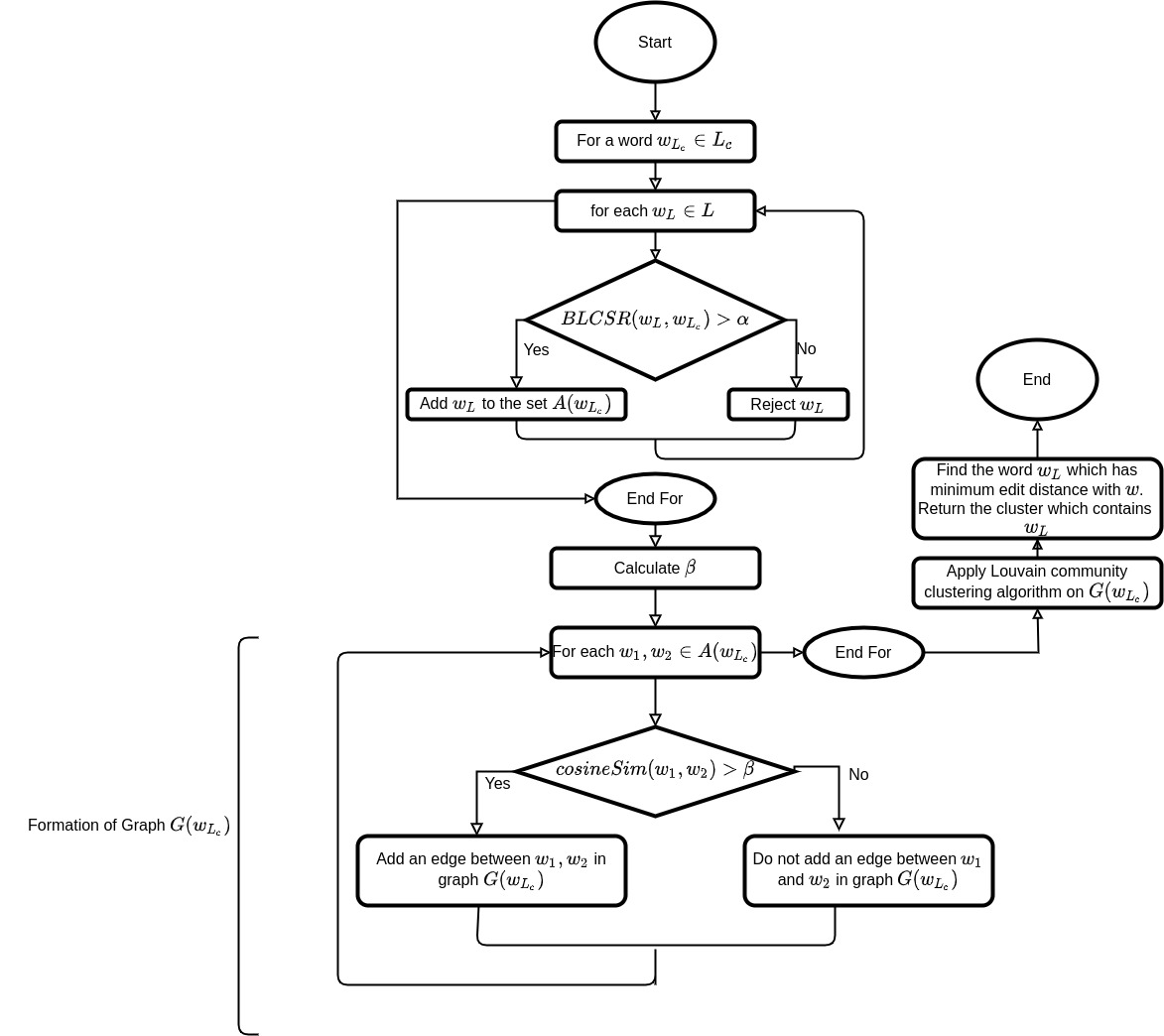
Figure 1: An overview of the proposed algorithm UnsupClean

Figure 1 shows an overview of our proposed algorithm UnsupClean. We explain each of the above steps in the following subsections.

3.2 Step 1: Generating a set of candidate morphological variants

For a given word $w_{L_{c}}$ (that is considered to be taken from the lexicon of correct words $L_{c}$), we first construct a set of morphological variants $A(w_{L_{c}})$, that would include all possible noisy variants of $w_{L_{c}}$ that occur in the given corpus. We observed that various noisy variants of words can be broadly classified into the following categories:
(1) Vowels are often added/deleted from words, especially in social media posts. E.g., ‘cool’ is written as ‘cooool’, and ‘thanks’ is written as ‘thnks’.
(2) Platforms like microblogging sites (e.g., Twitter, Weibo) allow very short posts, with a hard limit on the number of characters. On such platforms, users shorten words arbitrarily, omitting not only vowels but also many consonants. For instance, ‘tomorrow’ is shortened as ‘tmrw’, and ‘medicines’ as ‘meds’. Even named entities can be shortened, e.g., ‘Kathmandu’ as ‘ktm’ [5].
(3) People sometimes misspell words due to the phonetic similarity between the correct word and the misspelled word. For example, the phrase ‘smell like men’s cologne’ can be misspelled as ‘smell like men’s colon’.
(4) Different from the types of user-generated noise described above, there is also machine-generated noise (e.g., OCR noise) where spelling errors can occur in any part of the word (including the first character), whereas in case of human-generated variants, the first few characters usually match with that of the correct word. Also in case of OCR noise, there is a high chance of not having the correct word at all in the corpus, while a corpus containing user-generated errors usually contains both the clean and noisy variants of words.

To capture all these different types of noisy variants, we include in $A(w_{L_{c}})$, every word that has Bi-character Longest Common Sub-sequence Ratio (BLCSR) similarity with $w$ greater than a threshold $\alpha\in(0,1)$. Formally:

$$A(w_{L_{c}})=\{w_{L}\mid\textsc{BLCSR}(w_{L},w_{L_{c}})>\alpha\}$$ (1)

where $BLCSR$ is the Bi-character Longest Common Sub-sequence Ratio [23] based string similarity measure between two strings, and $\alpha\in(0,1)$ is a hyper-parameter. $BLCSR$ is $LCSR$ with bi-gram of characters calculated as:

$$BLCSR(w_{1},w_{2})=\frac{BLCS(w_{1},w_{2})}{maxlength(w_{1},w_{2})-1.0}$$ (2)

where $BLCS(w_{1},w_{2})$ is the Longest Common Subsequence considering bi-gram of characters. For example, if $w_{1}$ is ‘ABCD’ and $w_{2}$ is ‘ACD’ then its $BLCS$ value will be 1. Once $A(w_{L_{c}})$ is formed, we remove the word $w_{L_{c}}$ itself from $A(w_{L_{c}})$.

3.3 Step 2: Constructing a similarity graph of morphological variants

As stated earlier in this section, only string similarity based measure is not sufficient for capturing the morphological variations of words. Hence, we also consider the contextual similarity between words. We employ two ways of measuring contextual similarity between words – (i) observing co-occurrence counts. which works better for longer documents (that are more likely to contain multiple variants of the same word), and (ii) computing similarity between word embeddings which works better for short documents such as microblogs (since embeddings tend to lose the context over long windows).

Let $\overrightarrow{w_{i}}$ be the embedding of the word $w_{i}$. Specifically, we obtain the word embeddings using Word2vec [24] over the given corpus. Word2vec is a neural network based word-embedding generation model [24]. Unlike one-hot vectors for words, word2vec embeddings capture some contextual information in them – two words having similar word2vec embeddings have been used in similar context in the corpus on which Word2vec has been trained. For instance, after training word2vec on the ‘TREC 2005 confusion’ dataset, words like ‘program‘, ‘programs‘, ‘program1‘, and ‘program:s‘ have high cosine similarity amongst their embeddings. Here, a word $w_{i}$ is considered to be used in a similar context as another word $w_{j}$ if $w_{i}$ frequently appears ‘nearby’ $w_{j}$, i.e., within a fixed context window size around $w_{j}$. Another advantage of word2vec embeddings over one-hot vectors is that the size of these embeddings do not increase with increase in vocabulary. Two different versions of the Word2vec model exist depending upon how the embeddings are generated – (1) skip-gram, and (2) Continuous Bag of Words (CBoW). For our algorithm, we used Word2vec with context window size $3$ and skip-gram based approach. We chose skip-gram over CBoW since it generates better word embeddings in case of infrequent words. Also, we kept the context window size 3 so as to ensure good word embeddings for infrequent noisy words.

We construct a graph $G(w_{L_{c}})$ with all words from the set $A(w_{L_{c}})$ as the nodes. We consider an edge between two nodes (words) $w_{i},w_{j}\in A(w_{L_{c}})$ only if the value of cosine similarity between the embeddings $\overrightarrow{w_{i}}$ and $\overrightarrow{w_{j}}$ is greater than a threshold $\beta$. We calculate the $\beta$ value by using a weighted average of the cosine similarities between embeddings of all word-pairs in the set $A(w_{L_{c}})$, with the BLCSR value between the words as the corresponding weights. That is:

$$\beta=\frac{\sum_{w_{i},w_{j}\in A(w_{L_{c}})}BLCSR(w_{i},w_{j})*cosineSim(\overrightarrow{w_{i}},\overrightarrow{w_{j}})}{\sum_{w_{i},w_{j}\in A(w_{L_{c}})}BLCSR(w_{i},w_{j})}$$ (3)

This is done to find a threshold which takes both the syntactic similarity and semantic similarity into consideration. If $cosineSim(\overrightarrow{w_{i}},\overrightarrow{w_{j}})$ is greater than $\beta$, it means that the word-embedding model is highly confident of $w_{i}$ being a morphological variant of $w_{j}$ (and vice versa), and hence we connect the two words with an edge. We weight the edge between the two words $w_{i},w_{j}$ with weight $W_{ij}$ defined as:

$$W_{i,j}=cosineSim(\overrightarrow{w_{i}},\overrightarrow{w_{j}})\times Cooccur(w_{i},w_{j})$$ (4)

where $Cooccur(w_{i},w_{j})$ is the co-occurrence count of the words $w_{i}$ and $w_{j}$ in the same document (averaged over all documents in the corpus). We take the product of the two similarities since cosine-similarity of word embeddings captures similarity of the words in a local context (e.g., in a context window of size 3 words) and co-occurrence count captures their similarity in a global context (of a whole document).

3.4 Step 3: Fragmenting the graph into clusters of morphological variants

In the graph $G(w_{L_{c}})$, edges exist only between those nodes (words) which have at least a certain amount of similarity ($cosineSim(\overrightarrow{w_{i}},\overrightarrow{w_{j}})>\beta$). Next, we want to identify groups of words which have a high level of similarity among themselves. To this end, community detection or graph clustering algorithms can be used to identify groups of nodes that have ‘strong’ links (high-weight edges) among them. There are many graph clustering algorithms in literature [22]. We specifically use the popular Louvain graph clustering algorithm [25]. This algorithm functions on the principle of maximizing a modularity score [26] for each cluster/community, where the modularity quantifies the quality of an assignment of nodes to clusters, by evaluating how much more densely connected the nodes within a cluster are, compared to how connected they would be in a random network. Thus, it can be expected that all words in a particular cluster (as identified by Louvain algorithm) have strong semantic similarity amongst them.

3.5 Step 4: Finding the most suitable cluster for a word

Out of the clusters identified from $G(w_{L_{c}})$, we now need to find that cluster $Cl_{w_{L_{c}}}$ whose members are most likely to be the morphological variants of the given word $w_{L_{c}}$. We consider $Cl_{w_{L_{c}}}$ to be that cluster which contains the word with the minimum edit-distance from the word $w_{L_{c}}$ (ties broken arbitrarily).

Thus, for a given word $w_{L_{c}}$, we identify a set $Cl_{w_{L_{c}}}$ of morphological variants. Some examples of $Cl$s identified by the proposed algorithm are shown later in Table 6 and Table 7.

4 Baseline text normalization approaches

We compare the performance of our proposed text normalization algorithm with those of several baseline normalization methods that are described in this section. Since the implementations of these baselines are not publicly available (except Aspell and Enelvo), we implemented the algorithms following the descriptions in the respective papers, with some modifications as described below. Code for Enelvo is publicly available but as a normalizer package for Portuguese Language. Hence we implemented the Enelvo algorithm as well.

4.1 Aspell

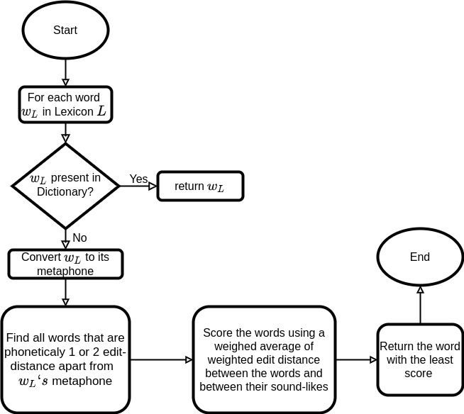
Figure 2: An overview of GNU Aspell

Aspell is an open-source spell checking library which uses a combination of Lawren Philips’ metaphone search algorithm [27] and Ispell’s missed strategy mechanism. Given a (misspelled) word, the algorithm first finds all the metaphones of the word. It then finds all the words that are within 1 or 2 edit-distance from any of the metaphones of the word. Figure 2 shows a flowchart describing the functioning of Aspell.

We used the GNU implementation of Aspell with the Python wrapper available at https://github.com/WojciechMula/aspell-python. For the RISOT dataset (in Bengali) that we use later in the paper, we used the Aspell Bengali dictionary available at https://ftp.gnu.org/gnu/aspell/dict/0index.html.

4.2 Sridhar

Unlike a spell-checker like Aspell, the approach by Sridhar [8] uses both contextual information and structural information for text normalization. Figure 3 gives a schematic flowchart describing the method.

The approach involves a lexicon $L_{c}$ of correct words (i.e. $w_{L_{c}}\in L_{c}$) such that there exists a word embedding for each $w_{L_{c}}$. Noisy versions for each $w_{L_{c}}$ are found from the corpus as:

$$\mbox{noisy-version}[w_{L_{c}}]=\displaystyle\forall_{w_{L}\in L,w_{L}\notin L_{c}}\,\max_{k}\mbox{cosineSim}(\overrightarrow{w_{L_{c}}},\overrightarrow{w_{L}})$$ (5)

where $w_{L}$ is a noisy word from the corpus $C$ with lexicon $L$. For each $w_{L_{c}}$, $k=25$ nearest neighbors are found and stored in the map noisy-version. Note that only contextual similarity among word embeddings is considered for identifying noisy versions in this initial step.

Now for a given noisy word $w_{L}\in L$, a list of all those $w_{L_{c}}$ is obtained for which noisy-version[$w_{L_{c}}$] contains $w_{L}$. The words $w_{L_{c}}$ in this list are scored, where the score is calculated as:

$$\mbox{score}(w_{L_{c}},w_{L})=\frac{LCSR(w_{L},w_{L_{c}})}{ED(w_{L},w_{L_{c}})}$$ (6)

where $ED(w_{L},w_{L_{c}})$ is the edit-distance between $w_{L}$ and $w_{L_{c}}$, and $LCSR(w_{L},w_{L_{c}})$ is the Longest Common Subsequence Ratio [23] calculated as

$$LCSR(w_{L},w_{L_{c}})=\frac{LCS(w_{L},w_{Lc})}{maxlength(w_{L},w_{L_{c}})}$$ (7)

where $LCS(w_{L},w_{L_{c}})$ is the Longest Common Subsequence Length between the words $w_{L}$ and $w_{L_{c}}$.

Finally, the $w_{L_{c}}$ with the highest score (as computed above) is considered to be the normalized version of the noisy word $w_{L}$. Note that the computation of score considers only the lexical similarity between words. The integration of contextual similarity with lexical similarity is achieved by first selecting the $w_{L_{c}}$ words based on contextual similarity with $w_{L}$, and then computing the lexical similarity score.

In the original paper [8], the author created $L_{c}$ (the lexicon of correct words) by training a word embedding model on some randomly selected sentences from the corpus which were manually normalized by a professional transcriber. Since our objective is to not use human resource, we chose pre-trained word-vectors to construct $L_{c}$. Specifically, for the RISOT dataset (in Bengali), we used pre-trained word2vec word vectors on Bengali Wikipedia data (available at https://github.com/Kyubyong/wordvectors), and for the English / microblog datasets, we used the pre-trained Word2Vec word vectors on the English Google News data (available at https://github.com/eyaler/word2vec-slim).

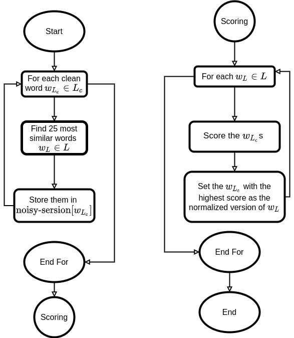
Figure 3: The overview of the algorithms of both Sridhar [8] and Enelvo [9]. The only difference between the two algorithms is the way in which the scores are calculated.

4.3 Enelvo

This method [9] is inherently similar to that of Sridhar [8]. Figure 3 gives a schematic flowchart describing both these methods. Enelvo involves a lexicon $L_{c}$ of correct words (i.e., $w_{L_{c}}\in L_{c}$) with frequency $\geq 100$ in the given corpus. The noisy versions $w_{L}\in L$ (the lexicon the given corpus) of the word $w_{L_{c}}$ are then found as:

$$\mbox{noisy-version}[w_{L_{c}}]=\displaystyle\forall_{w_{L}\in L,w_{L}\notin L_{c}}\,\max_{k}\mbox{cosineSim}(\overrightarrow{w_{L_{c}}},\overrightarrow{w_{L}})$$ (8)

where $w_{L_{c}}$ is the correct word from the lexicon $L_{c}$, and $w_{L}$ is the noisy word from the lexicon $L$ of corpus $C$. For each $w_{L_{c}}$, the top $k=25$ most similar noisy words $w_{L}\in L$ are found and stored in the map noisy-version. This step is similar to the first step in the Sridhar baseline [8], and considers only contextual similarity among word embeddings.

Next, for a given noisy word $w_{L}\in L$ a list of all those $w_{L_{c}}$ is chosen for which noisy-version[$w_{L_{c}}$] contains $w_{L}$. The words $w_{L_{c}}$ in this list are then scored.

The score is computed as:

$$score(w_{L},w_{L_{c}})=n\times\mbox{lexical-similarity}(w_{L},w_{L_{c}})+(1-n)\times\mbox{cosineSim}(\overrightarrow{w_{L}},\overrightarrow{w_{L_{c}}})$$ (9)

where $n\in(0,1)$ is a hyperparameter, and lexical-similarity($w_{L},w_{L_{c}}$) is measured as:

$$\mbox{lexical-similarity}(w_{L},w_{L_{c}})=\begin{cases}\frac{LCSR(w_{L},w_{L_{c}})}{MED(w_{L},w_{L_{c}})},&\text{if $MED(w_{L},w_{L_{c}})>0$}.\\ LCSR(w_{L},w_{L_{c}}),&\text{otherwise}.\end{cases}$$ (10)

Here $MED(w_{L},w_{L_{c}})=ED(w_{L},w_{L_{c}})-DS(w_{L},w_{L_{c}})$ is the modified edit distance between $w_{L}$ and $w_{L_{c}}$, where $ED(w_{L},w_{L_{c}})$ is the edit distance and $DS(w_{L},w_{L_{c}})$ is the diacritical symmetry between $w_{L}$ and $w_{L_{c}}$ (a feature that is useful in Portuguese and some non-English languages – see [9] for details). $LCSR(w_{L},w_{L_{c}})$ is the Longest Common Subsequence Ratio, calculated as:

$$LCSR(w_{L},w_{L_{c}})=\frac{LCS(w_{L},w_{L_{c}})+DS(w_{L},w_{L_{c}})}{maxlength(w_{L},w_{L_{c}})}$$ (11)

where $LCS(w_{L},w_{L_{c}})$ is the Longest Common Subsequence of words $w_{L}$ and $w_{L_{c}}$. Hence, the computation of score integrates both lexical similarity as well as contextual similarity, which is a point of difference from the Sridhar baseline [8]. Finally, the $w_{L_{c}}$ with the highest score is chosen as the normalized version of $w_{L}$.

Thus, the integration of contextual similarity and lexical similarity is achieved in Enelvo as follows – first, the top $k$ noisy words $w_{L}$ are chosen for each clean word $w_{L_{c}}$ using contextual similarity. Then for a given noisy word $w_{L}$, the best clean word $w_{L_{c}}$ is selected using a scoring function that is a weighted combination of contextual similarity and lexical similarity.

For the embeddings, the authors of [9] trained a Word2Vec skip-gram model on a conglomeration of two corpora – Twitter posts written in Portuguese and a product review corpus containing both noisy and correct texts [28]. Since our datasets are in English and Bengali, we used pre-trained embeddings for the correct words $w_{L_{c}}\in L_{c}$ and trained word2vec models on the respective noisy corpora for the noisy word embeddings $w_{L}\in L$. For the embeddings of $w_{L_{c}}$ in the RISOT dataset, we used pretrained Word2Vec embeddings of the Bengali Wikipedia dataset (available at https://github.com/Kyubyong/wordvectors). Similarly, for the English and microblog datasets, we used pretrained word embeddings of the Google English News dataset (available at https://github.com/eyaler/word2vec-slim).

4.4 Ghosh

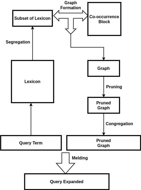
Figure 4: An overview of the algorithm by Ghosh et. al., derived from the original paper [7]

Ghosh et. al [7] employs a five-step approach to find the morphological variants of a word (see Figure 4). The first step called segregation involves removal of words with string similarity $\leq\alpha$ (where $\alpha\in(0,1]$) with the correct word $w_{L_{c}}$(or query word), resulting in the formation of $A(w_{L_{c}})$. The next step is Graph Formation where a graph $G=(V,E)$ is formed with vertices $V$ as the words in $A(w_{L_{c}})$ and edges $E$ with weights as the co-occurrence counts between them. Next step is the Pruning step where the Graph $G$ is pruned. Pruning is carried out only if the maximum edge-weight ($max_{ew}$) in $G$ is greater than a threshold $\gamma$ which is determined by the user. In this step, edges which are less than $\beta\;\%$ of $max_{ew}$ are removed from the Graph $G$ resulting in the formation of a graph $G_{r}=(V,E^{\prime})$ where $E^{\prime}\subset E$.

The next step is called Congregation where the graph $G_{r}$ is further fragmented into clusters based on their edge-weights. Two vertices $v_{1}$ and $v_{2}$ belong to the same cluster if they satisfy any of the following conditions – (i) $v_{1}$ is the strongest neighbour of $v_{2}$, or (ii) $v_{2}$ is the strongest neighbour of $v_{1}$. This results in the formation of a set of $k$ clusters $CL=\{Cl_{1},Cl_{2},\ldots,Cl_{k}\}$. Congregation step is followed by the final step called Melding. In this step, a cluster is chosen from the set of clusters $CL$ to have the morphological variants of the query word $w_{L_{c}}$. Such a cluster containing lexically the most similar word to $w_{L_{c}}$ is chosen to be the cluster containing morphological variants of $w_{L_{c}}$. The lexical similarity is measured using Edit Similarity (ES), which is an edit-distance based similarity metric, having the formula:

$$ES(w_{1},w_{2})=1-\frac{ED(w_{1},w_{2})}{max(stringLength(w_{1}),stringLength(w_{2}))}$$ (12)

where $ED(w_{1},w_{2})$ is the edit-distance between the two words $w_{1}$ and $w_{2}$.

Difference of proposed algorithm with baselines: The baseline normalization algorithms discussed in this section are significantly different from the proposed algorithm UnsupClean. Sridhar and Enelvo both use contextual and lexical similarity, as does UnsupClean; however, the approach for integrating contextual similarity and lexical similarity is different in UnsupClean as compared to Sridhar and Enelvo. Additionally, neither Sridhar nor Enelvo are graph-based methods, whereas UnsupClean relies on forming a similarity graph and then clustering the graph. The Ghosh baseline is most similar to UnsupClean – both use contextual as well as lexical similarity, and both are graph-based methods. But importantly, Ghosh measures contextual similarity using only co-occurrence statistics, whereas UnsupClean uses a combination of co-occurrence statistics and word embeddings. The advantage of using word embeddings will be clear from our experiments described in the subsequent sections.

In the next two sections, we compare the performance of the proposed UnsupClean text normalization algorithm with that of the baseline normalization algorithms described in this section. To this end, we consider two downstream applications – retrieval (Section 5) and stance detection (Section 6).

5 Downstream Application 1: Retrieval

In this section, we evaluate the performance of a text normalization algorithm by observing the performance of a retrieval (search) system over a noisy corpus that is normalized by the algorithm.

5.1 Datasets for retrieval

For evaluation of various text normalization methods, we experimented with the following three datasets, each having a different source of noise. The statistics of the datasets are given in Table 2.

(1) RISOT Bengali OCR Data: This dataset was released in the FIRE RISOT track (https://www.isical.ac.in/~fire/risot/risot2012.html). The text version of 62,825 news articles of a premiere Bengali newspaper Anandabazar Patrika (2004-2006) was scanned and OCRed to create the collection. The dataset also contains 66 queries, and their set of relevant documents (gold standard).

(2) TREC 2005 Confusion Track Data: This dataset was created for the TREC Confusion track 2005 [29]. The dataset consists of the text versions of Federal Register English documents (of the year 1994), which were scanned and OCR-ed. We use the 5% version for our experiments, where the approximate character error rate is 5%. Further details can be found in [29].

Dataset	No. of documents	No. of queries
FIRE RISOT Bengali	62,825	66
TREC Confusion 2005	55,600	49
TREC Microblog 2011	16,074,238	50

Table 2: Description of the retrieval datasets used for empirical comparison of the proposed and baseline text normalization methods.

(3) TREC 2011 Microblog Track Data: We consider an English tweet collection viz. TREC Microblog track collection 2011 (https://trec.nist.gov/data/microblog2011.html, containing noise produced by cavalier human writing style. Unlike the other two datasets, this is a much larger collection (containing over 16 million tweets), and is also expected to test the scalability of any text normalization method.

Thus, we use three noisy collections having different types of errors (OCR errors, errors due to users’ writing styles) in two different languages (English and Bengali) to test the efficacy and language independence of various text normalization methods. For brevity, we refer to the datasets as RISOT, Confusion and Microblog respectively.

5.2 Retrieval Model used

We used the popular Information Retrieval system Indri which is a component of the Lemur Toolkit (https://www.lemurproject.org/indri/) for the retrieval experiments. Indri is a language-independent retrieval system, that combines language modeling and inference network approaches [30]. We used the default setting of Indri for all experiments.

A particular corpus is first normalized using a normalization algorithm (either UnsupClean, or one of the baselines Sridhar, Enelvo, Ghosh, and Aspell), and the normalized corpus is then indexed using Indri. The queries are also normalized using the same normalization algorithm, and then the retrieval is carried out.

5.3 Parameter settings of normalization algorithms

The proposed algorithm has one hyperparameter $\alpha$ (the similarity threshold for BLCSR). We obtained the best value for $\alpha$ via grid search in the range $[0.5,1.0]$ with a step size of $0.01$. The best values are $\alpha=0.56$ for RISOT, $\alpha=0.9$ for Confusion and $\alpha=0.83$ for the Microblog dataset.

Ghosh et al. [7] has three hyper-parameters, namely $\alpha,\beta$ and $\gamma$. We followed the same methodology as stated in the original paper [7] to set the parameters – we varied the $\alpha$ and $\beta$ while keeping the $\gamma$ value equal to $50$. We obtained the best values for $\alpha$ and $\beta$ via grid search in the range $[0.5,1.0]$ with a step size of $0.01$. The best values are $\alpha=0.8,\beta=0.7$ for RISOT, $\alpha=0.9,\beta=0.7$ for TREC 2011 microblog and $\alpha=0.7,\beta=0.8$ for the Confusion dataset.

For both Sridhar [8] and Enelvo [9] have a hyper-parameter $K$ (the number of nearest neighbors to a particular word $w$, that are considered as potential variants of $w$).

Both these works directly specify $k=25$ without any tuning. Hence, we adhered to the value $k=25$ value provided by the authors in their papers. Enelvo has another hyper-parameter $n$ that specifies the relative significance of contextual similarity and lexical similarity while computing score; we used $n=0.8$, the value used by the authors in the original paper.

5.4 Evaluation metrics for retrieval

As stated earlier, to evaluate the performance of a text normalization algorithm, we measure the performance of retrieval on noisy datasets (described in Section 5.1) cleaned using the normalization algorithm. We use some standard metrics to evaluate the retrieval performance, as follows.

For the RISOT and Microblog datasets, we measure Recall@100 (at rank 100), Mean Average Precision mAP@100 and mAP@1000 (at ranks 100 and 1000) as the metrics for comparing the retrieval performance.

The TREC 2005 Confusion dataset, however, has only one relevant document per query. Hence, it is more common to report the Mean Reciprocal Rank (MRR) metric for this dataset.

5.5 Results

Table 3 compares the retrieval performance using different text normalization algorithms (the proposed method and the baselines) for the RISOT Bengali dataset. Also shown are the retrieval performances over the raw data, i.e., without any normalization. Similarly, Table 4 shows the results for the TREC 2011 Microblog dataset, while Table 5 shows results for the TREC 2005 Confusion dataset. The tables also report results of statistical significance testing – the symbols A, E, G, S in the superscripts in the tables indicate that the proposed method is statistically significantly better at 95% confidence interval ($p<0.05$) than Aspell, Enelvo, Ghosh et al., and Sridhar respectively.

For the Microblog dataset (see Table 4), the proposed UnsupClean performs competitively with the baselines. Retrieval using the Sridhar baseline achieves higher Recall@100, while retrieval using UnsupClean achieves higher mAP@100 and mAP@1000 scores. None of the differences are statistically significant.

For the other two datasets which primarily contain OCR noise (see Table 3 and Table 5), UnsupClean enables much better retrieval than the baselines. Especially for the RISOT dataset (in Bengali language), the baselines Enelvo, Sridhar and Aspell perform very poorly. In fact, in most cases, retrieval performance is better over the raw RISOT data, than after normalization by these three baselines. In contrast, UnsupClean leads to significant improvement in retrieval performance. Hence, the proposed model can generalize to different types of noise as well as different languages, better than most of the baselines.

Normalization Algorithm	Recall@100	mAP@100	mAP@1000
Raw data (without any cleaning)	50.08%	17.21%	18.50%
Ghosh et al.[7]	54.48%	19.48%	20.98%
Enelvo [9]	49.24%	17.04%	18.37%
Sridhar [8]	47.75%	17.38%	18.76%
Aspell	24.40%	5.43%	5.58%
UnsupClean (Proposed)	58.32%ESA	21.50%ESA	23.00%ESA

Table 3: Retrieval performance on RISOT Bengali OCR dataset, using Indri IR system. Best performances are in bold font. Superscripts E,S,A indicate the proposed method is statistically significantly better than Enelvo, Sridhar and Aspell respectively.

Normalization Algorithm	Recall@100	mAP@100	mAP@1000
Raw data (without any cleaning)	37.63%	16.13%	19.77%
Ghosh et al.[7]	37.62%	15.97%	19.66%
Enelvo [9]	38.79%	15.84%	19.39%
Sridhar [8]	39.79%	16.20%	19.91%
Aspell	23.28%	9.68%	12.44%
UnsupClean (Proposed)	39.23%	16.34%	20.01%

Table 4: Retrieval performance on TREC 2011 microblog dataset, using Indri IR system. Best performances are in bold font (none of the differences in performance are statistically significant).

Normalization Algorithm	Mean Reciprocal Rank
Raw data (without any cleaning)	62.93%
Ghosh et al.[7]	63.78%
Enelvo [9]	55.20%
Sridhar [8]	54.36%
Aspell	38.93%
UnsupClean (Proposed)	70.21%ESA

Table 5: Retrieval Performance on TREC 2005 Confusion dataset, using Indri IR system. Best result are in bold font. Superscripts E,S,A indicate the same as in Table 3.

5.6 Comparative Analysis

Out of all the text normalization algorithms, retrieval using Aspell performs most poorly. In general, spelling correction algorithms such as Aspell are unable to segregate words with high string similarity but low semantic similarity (‘industrious’ and ‘industrial’), or homonyms (such as ‘living’ and ‘leaving’), etc. Such variants can be identified by the proposed algorithm as well as by the other baselines which use context information in identification of variants.

In the rest of this section, we report some insights on how the proposed UnsupClean model differs from the other baselines Sridhar [8], Enelvo [9] and Ghosh et al. [7]. For this analysis, Table 6 and Table 7 show some examples of morphological variants identified by these algorithms for the same word.

UnsupClean vs Sridhar/Enelvo: Both Sridhar and Enelvo first consider the contextual similarity for identifying a candidate set of morphological variants (see Eqn. 5 and Eqn. 8 in the descriptions of Sridhar and Enelvo respectively). They initially ignore the structural/lexical similarity between words, which at times includes incorrect variants into the candidate set. For instance, the word ‘turmeric’ is identified as a candidate variant of ‘organic’ by Enelvo, while the words ‘nbcnews’ and ‘tpmdc’ are identified by both the methods as candidate variants of ‘msnbc’ (see Table 6), due to the high contextual similarity between these words. On the other hand, the proposed method considers $w_{j}$ to be a candidate variant of $w_{i}$ only if their lexical similarity is higher than a threshold; hence, such wrong variants are not included in $A(w_{i})$ (on which contextual similarity is later applied).

Word	UnsupClean	Ghosh	Enelvo	Sridhar
release	release, released, releases	release	release, realease, relea	releasing, released, realease, release, releases, relea
organic	organic, organik, organi	organic	turmeric, organic	organic
msnbc	msnbc	msnbc	cbsnews, tpmdc, msnbc, foxnews, nbcnews	msnbc, nbcnews, cbsnews, tpmdc, masrawy

Table 6: Resulting clusters of morphological variants of some specific query-words, on the TREC 2011 microblog dataset

Word	UnsupClean	Ghosh	Enelvo	Sridhar
program	programt, 44program, programs, program1, program programs1, sprogram, program11,	program, programs	program programs1, program1, programs, prodects	programs, program, programs1
document	document1, documents, documents1, locument1, locuments, locument, document, locuments1	documents, document	document, forepart, locument, document1, documents	locument, documents, document1, document

Table 7: Resulting clusters of morphological variants of some specific query-words, on the TREC 2005 Confusion dataset

UnsupClean vs. Ghosh et al.: Ghosh et al. [7] computes the contextual similarity among words using only the co-occurrence counts of words in the same document. This method works well for long documents having a small vocabulary, but performs poorly when the vocabulary size is very large or when the document size is very small (in which case the co-occurrence matrix will be very sparse). Especially, two error variants of the same word rarely co-occur in the same microblog. Hence, Ghosh et. al [7] performs well on the RISOT dataset, but poorly on the Microblog and Confusion datasets. On the other hand, the proposed method employs both co-occurrence counts and cosine similarity of embeddings to capture contextual similarity among words, and hence generalizes better to different types of noise and documents.

5.7 Ablation Analysis

Normalization Algorithm	Recall@100	mAP@100	mAP@1000
UnsupClean (with all components)	58.3%	21.5%	23.0%
UnsupClean without $\beta$ thresholding	57.0	20.3	21.5
UnsupClean without similarity graph of morphological variants	54.9	18.6	19.1
UnsupClean without graph fragmentation	52.6	19.1	20.7

Table 8: Ablation analysis of UnsupClean – how retrieval performance (on RISOT Bengali OCR dataset, using Indri IR system) varies with removal of various components.

We conducted an ablation analysis in order to understand the importance of various steps / components in our algorithm. To this end, we applied UnsupClean on the RISOT dataset in various settings – with all steps, and by removing one step at a time. Table 8 shows the results of the ablation analysis.

The $\beta$ thresholding (see Step 2 in Section 3.3) is done to consider words which have a high contextual similarity only. This is done to ensure high precision of the retrieved results. As can be seen from Table 8, the removal of such a threshold results in the drop of mAP scores. The recall@100, however, does not reduce much, since the morpheme cluster increases.

The construction of similarity graph of morphological variants (see Step 2 in Section 3.3) is a crucial step that helps capture the contextual similarity among words with different morphological structures. Removal of this step will result in a significant drop in both mAP and recall scores compared to UnsupClean.

If the graph fragmenting step (see Step 3 in Section 3.4) is skipped, we miss out on identifying the strongly connected component of the graph, and thus weakly connected components also get drawn into the final cluster, causing a decrease in both mAP as well as recall scores.

This ablation analysis shows that all the steps of the UnsupClean algorithm are essential, and removing any of the steps will adversely affect the retrieval performance. Especially, skipping the graph formation step leads to substantial degradation in both Precision and Recall of retrieval. Also the graph fragmenting step is crucial particularly for Recall.

From the experiments and analyses stated in this section, we can conclude the our proposed algorithm UnsupClean is very helpful in enhancing retrieval from noisy text. UnsupClean out-performs almost all baselines across different types of noisy corpus (containing OCR noise, and noise due to cavalier writing style of human users) and across multiple languages (English and Bengali). Especially for corpus with OCR noise, UnsupClean enables statistically significantly better retrieval than most baselines, while it achieves very competitive performance in case of noisy microblogs. Additionally, UnsupClean is completely unsupervised, and does not need any manual intervention at any step, thus making it suitable for use on large corpora in various languages.

6 Downstream Application 2: Stance Detection

Online platforms such as Twitter, Facebook, etc. have become popular forums to discuss about various socio-political topics and express personal opinions regarding these topics. In this kind of scenario, ‘stance’ refers to the inherent sentiment express by an opinion towards a particular topic. The topic is referred to as the ‘target’. The ‘stance’ expressed by a blog/tweet can have three types of sentiment towards a given topic. It can either support (or favor) the target, it can oppose (or be against) the target, or it can be neutral, i.e., neither support nor oppose the target. The problem of ‘stance detection’ refers to the process of automatically identifying this stance or sentiment of a post expressed towards a target. The reader is referred to [31] for a recent survey on stance detection.

Stance detection is frequently carried out on crowdsourced data such as tweets/blogs which are noisy in nature, due to frequent use of informal language, non-standard abbreviations, and so on. There exist several popular methods for stance detection from such noisy crowdsourced content. In this section, we check whether using text normalization algorithms improves the performance of these stance detection models on noisy microblogs.

6.1 Datasets for stance detection

We consider datasets made available by the SEMEVAL 2016 Task 6A challenge [4] which are commonly used datasets for stance detection, and have been used in a number of prior works. The datasets consist of tweets (microblogs) for different topics; for each topic, there are three types of tweets – those in favor of (supporting) the topic, those against (opposing) the topic, and tweets that are neutral to the topic. We consider the following three SemEval datasets:
(i) Atheism (AT): Here the target is ‘atheism’, and the tweets are in favor of, or against the idea of atheism (or neutral).
(ii) Climate change is a real concern (CC): For this dataset the target is ‘Climate change is a real concern’.
(iii) Hillary Clinton (HC): Here the target is ‘Hillary Clinton’, and the tweets are either in support of / against the politician.
We refer to these datasets as AT, CC and HC respectively for brevity in the rest of the paper.

The datasets are already partitioned into train and test sets, as defined in the SEMEVAL 2016 Task 6A challenge [4]. The numbers of tweets in each dataset is stated in Table 9. We have also provided some examples of tweets in the datasets in Table 10.

Dataset	# Training Instances			# Test Instances
	Favor	Against	Neutral	Favor	Against	Neutral
SemEval-AT	92	304	117	32	160	28
SemEval-CC	212	15	168	123	11	35
SemEval-HC	112	361	166	45	172	78

Table 9: Statistics of standard SEMEVAL 2016 Task 6A datasets for stance detection (divided into training and test sets).

Tweet text	Label
Tweets from SemEval-AT (Atheism) dataset
Absolutely f**king sick & tired of the religious and their "We’re persecuted" bollocks​ So f**king what? Pissoff! #SemST	FAVOR
All that is needed for God for something to happen is to say "#Be" and it is; for God is capable of all things. #God created #trinity #SemST	AGAINST
In other related news. Boko Haram has killed over 200 people in the last 48hrs. #SemST	NEUTRAL
Tweets from SemEval-CC (Climate Change is a Real Concern) dataset
We cant deny it, its really happening. #SemST	FAVOR
The Climate Change people are disgusting a**holes. Money transfer scheme for elite. May you rot. #SemST	AGAINST
@AlharbiF I’ll bomb anything I can get my hands on, especially if THEY aren’t christian. #graham2016 #GOP #SemST	NEUTRAL
Tweets from SemEval-HC (Hillary Clinton) dataset
@HuffPostPol If @HillaryClinton can do half of what he did then she would be doing is a favor #SemST	FAVOR
Although I certainly have disagreements, after reading about @GovernorOMalley I much rather have him than @HillaryClinton. #SemST	AGAINST
Lets remember #dickcheney is an unindicted war criminal b4 we start yelling #Benghazi day after day. Will we ever see justice? #SemST	NEUTRAL

Table 10: Examples of posts from the SemEval datasets. Some characters in abusive words are replaced with *

6.2 Stance Detection Models

We consider two stance detection models for the experiments.

1. LSTM (Long Short Term Memory): This model was proposed by Hochreiter and Schmidhuber [32] to specifically address this issue of learning long-term dependencies. The LSTM maintains a separate memory cell inside it that updates and exposes its content only when deemed necessary.A number of minor modifications to the standard LSTM unit have been made. We define the LSTM units at each time step t to be a collection of vectors in $R^{d}$ : an input gate $i_{t}$, a forget gate $f_{t}$, an output gate $o_{t}$, a memory cell $c_{t}$, and a hidden state $h_{t}$ . $d$ is the number of the LSTM units. The entries of the gating vectors $i_{t}$, $f_{t}$ and $o_{t}$ are in $[0,1]$. The LSTM transition equations are the following:

   $$i_{t}=\sigma(W_{i}x_{t}+U_{i}h_{t-1}+V_{i}c_{t-1})$$ (13)

   $$f_{t}=\sigma(W_{f}x_{t}+U_{f}h_{t-1}+V_{f}c_{t-1})$$ (14)

   $$o_{t}=\sigma(W_{o}x_{t}+U_{o}h_{t-1}+V_{o}c_{t-1})$$ (15)

   $$\tilde{c}_{t}=\sigma(W_{i}x_{t}+U_{i}h_{t-1}+V_{i}c_{t-1})$$ (16)

   $$c_{t}=f_{t}\odot c_{t-1}+i_{t}\odot\tilde{c}_{t}$$ (17)

   $$h_{t}=o_{t}\odot tanh(c_{t})$$ (18)

   For detecting stance , a simple strategy is to map the input sequence to a fixed-sized vector using one RNN, and then to feed the vector to a softmax layer. Given a text sequence, x=$[x_{1},x_{2}$,···$,x_{T}]$, we first use a lookup layer to get the vector representation (embeddings) of each word $\mathbf{x}_{i}$. The output $\mathbf{h}_{T}$ can be regarded as the representation of the whole sequence, which has a fully connected layer followed by a softmax non-linear layer that predicts the probability distribution over stances (in this case either ‘FAVOR’ or ‘AGAINST’ or ‘NEUTRAL’). The LSTM model has the following hyperparameters whose values are taken as follows: learning rate of $5\times e^{-4}$ and dropout of $0.5$.

2. Target Specific Attention Neural Network (TAN): This model was introduced by Du et al. [33], one of the winning entries SemEval 2016 task 6A [4] challenge. The model is based on bidirectional LSTM with an attention mechanism. A target sequence of length $N$ is represented as $[z_{1},z_{2},\ldots,z_{N}]$ where $z_{n}\epsilon R^{d^{{}^{\prime}}}$ is the $d^{{}^{\prime}}$-dimensional vector of the $n$-th word in the target sequence. The target-augmented embedding of a word $t$ for a specific target $z$ is $e^{z}_{t}=x_{t}\odot z$ where $\odot$ is the vector concatenation operation. The dimension of $e^{z}_{t}$ is $(d+d^{{}^{\prime}})$. An affine transformation maps the $(d+d^{{}^{\prime}}$)-dimensional target-augmented embedding of each word to a scalar value as per the following Eqn. 19:

   $$a^{{}^{\prime}}_{t}=W_{a}e_{t}^{z}+b_{a}$$ (19)

   where $W_{a}$ and $b_{a}$ are the parameters of the bypass neural network. The attention vector $[a^{{}^{\prime}}_{1},a^{{}^{\prime}}_{2},\ldots,a^{{}^{\prime}}_{T}]$ undergoes a softmax transformation to get the final attention signal vector (Eqn. 20):

   $$a_{t}=softmax(a_{t})=\frac{e^{a^{{}^{\prime}}_{t}}}{\sum_{i=1}^{T}e^{a^{{}^{\prime}}_{i}}}$$ (20)

   After this, the product of attention signal $a_{t}$ and $h_{t}$ (which is the corresponding hidden state vector of RNN) is used to represent the word t in a sequence with attention signal. The representation of the whole sequence can be obtained by averaging the word representations:

   $$s=\frac{1}{T}\sum_{t=0}^{T}a_{t}h_{t}$$ (21)

   where $s$ $\epsilon$ $R^{d}$ is the vector representation of the text sequence and it can be used as features for text classification:

   $$p=softmax(W_{clf}s+b_{clf})$$ (22)

   where $p$ $\epsilon$ $R^{C}$ is the vector of predicted probability for stance. Here $C$ is the number of classes of stance labels, and $W_{clf}$ and $b_{clf}$ are parameters of the classification layer.

   The TAN model has two hyperparameters, whose values are taken as follows: learning rate of $5\times e^{-4}$ and dropout of $0.5$.

6.3 Parameter settings of normalization algorithms

We set the parameters for various text normalization algorithms in a way similar to what was described in Section 5.3. For the proposed method, the value of $\alpha$ is set of $0.56$. For Ghosh et al. [7], the parameters were set to $\alpha=0.7,\beta=0.6,\gamma=50$ (decided through grid search, as described in Section 5.3). For Sridhar [8] and Enelvo [9], the hyperparameter $K$ was set to $25$ as specified in the original papers. For Enelvo [9], $n$ was set to $0.8$.

6.4 Evaluation Metric for stance detection

To evaluate the performance of different models, we use the same metric as reported by the official SemEval 2016 Task A [4]. We use the macro-average of the F1-score for ‘favor’ and ‘against’ as the bottom-line evaluation metric.

$$F_{avg}=\frac{F_{favor}+F_{against}}{2}$$ (23)

where $F_{favor}$ and $F_{against}$ are calculated as shown below:

$$F_{favor}=\frac{2P_{favor}R_{favor}}{P_{favor}+R_{favor}}$$ (24)

$$F_{against}=\frac{2P_{against}R_{against}}{P_{against}+R_{against}}$$ (25)

Here $P_{favor}$ and $R_{favor}$ are the precision and recall of the ‘FAVOR’ class respectively, and $P_{against}$ and $R_{against}$ respectively are the precision and recall of the ‘AGAINST’ class and are defined as:

$$P_{favor}=\frac{\#TP_{favor}}{\#TP_{favor}+\#FP_{favor}}$$ (26)

$$R_{favor}=\frac{\#TP_{favor}}{\#TP_{favor}+\#FN_{favor}}$$ (27)

$$P_{against}=\frac{\#TP_{against}}{\#TP_{against}+\#FP_{against}}$$ (28)

$$R_{against}=\frac{\#TP_{against}}{\#TP_{against}+\#FN_{against}}$$ (29)

With respect to ‘FAVOR’ class, $\#TP_{favor}$ refers to number of true positives in favor class, i.e., the number of tweets that are predicted as ‘FAVOR’ by the classifier, and are actually of ‘FAVOR’ class. $\#FP_{favor}$ refers to number of tweets which are not actually of ‘FAVOR’ class, but that have been predicted as ‘FAVOR’ by the classifier. $\#FN_{favor}$ refers to number of tweets which are actually of ‘FAVOR’ class but have been wrongly classified by the classifier.

6.5 Results

The experiments with a particular dataset are as follows. Five instances of the dataset are normalized, one by each of the five normalization algorithms (UnsupClean and four baselines). The training set and the test set are normalized separately. Subsequently, a stance detection model (LSTM or TAN) is used on the normalized versions, and their performances are measured.

Table 11 shows the performance of the TAN stance detection model [33], on different versions of the datasets normalized by the different normalization algorithms. Also shown are the values on the raw datasets, i.e., without any cleaning. From Table 11, it can be seen that all normalization approaches lead to some improvement, as compared to the performance on the raw data. It is evident that the TAN model performs the best by using our proposed normalization method, for all three datasets (best metric values highlighted in boldface).

Similarly, Table 12 shows the performance of the LSTM [32] model on different versions of the datasets normalized by the different normalization algorithms, as well as on the raw dataset. The LSTM model performs the best by using the proposed normalization method for two datasets (AT and CC), and gives the second-best result for the HC dataset.

We checked the statistical significance of the differences in performance with various normalization methods using McNemar’s test (https://machinelearningmastery.com/mcnemars-test-for-machine-learning/); however, the differences in performance are not statistically significant.

Normalization Method	AT	CC	HC
Raw data (without any cleaning)	0.5508	0.3968	0.4396
Enelvo [9]	0.5659	0.4427	0.5336
Sridhar [8]	0.5476	0.4778	0.5318
Ghosh et al. [7].	0.6156	0.4641	0.5216
Aspell	0.5923	0.5250	0.4586
UnsupClean (Proposed)	0.6250	0.5271	0.5405

Table 11: Stance detection results on SemEval datasets by the TAN model [33]. The metric is as explained in Section 6.4. Highest values marked in boldface.

Normalization Method	AT	CC	HC
Raw data (without any cleaning)	0.5497	0.3760	0.4938
Enelvo [9]	0.6084	0.3911	0.5646
Sridhar [8]	0.5666	0.4558	0.5055
Ghosh et al. [7].	0.6395	0.3884	0.4893
Aspell	0.5902	0.4008	0.5337
UnsupClean (Proposed)	0.6411	0.4882	0.5401

Table 12: Stance classification results on SemEval datasets by the LSTM [32] model. The metric is as explained in Section 6.4. Highest values marked in boldface.

6.6 Analysis of result of stance detection

Table 13 shows some examples of tweets from the SemEval datasets, where all/most of the baseline normalization algorithms led to wrong stance detection by the TAN [33] model (for the first two examples) and by the LSTM model [32] (for the last two examples), but by using the proposed normalization method, the correct stance was identified for each of these tweets.

The first and third examples show a situation where the proposed UnsupClean keeps the words present in a tweet unchanged, but the baseline normalization methods change the words to some non-contextual variants that seem illogical and lead to wrong stance detection. In the second example the proposed method changes the phrase ‘thank you so much for’ to ‘thank you so much your’ whereas the modifications of different words by the other normalization methods seem wrong, such as from ‘@EstadodeSats’ to ‘stardust’s’ by Aspell, or from ‘thank’ to ’thang’ by Enelvo. A similar scenario is observed in the fourth example. Thus, the proposed model performs slightly better in understanding which words to modify (into variants) and which words to leave unchanged.

From the experiments described in this section, it can be concluded that the proposed text normalization algorithm UnsupClean competes very favorably with the baseline normalization models, for the stance detection task. We demonstrate the efficacy of UnsupClean with two popular stance detection models. Experiments show that both stance detection models perform better after text normalization with UnsupClean, as compared to text normalization with the baseline models.

These results, along with the results of retrieval in the previous Section 5, show that text normalization using UnsupClean enables superior performance in multiple text processing tasks.

Tweets from SemEval Datasets	UnsupClean (Proposed)	Enelvo [9]	Sridhar [8]	Ghosh et al. [7]	Aspell
Jesus response to a religious environment was to create a royal environment. It drove people nuts. Still does - thank God #SemST	jesus, religious, create	janus, Seditious, create	joss, regs, create	jesus, religious, creative	jesus, religious, create, replaces ‘#’ by ‘W’
@csham21 @EstadodeSats Thank you so much for supportive #Freedom4Cuba RTs! #WakeUpAmerica #Cuba #TodosMarchamos #SemST	estadodesats, thank you, much your	estadodesats, thang Lou, guch onr	estadodesats, thanks yU, mce onr	estadodesats, anything 4your, much 4your	stardust’s, thank you, much for, replaces ‘#’ by ‘W’
.@mite72 @PatVPeters NEITHER ONE!!!! Just making a funny! #SemST	patvpeters, one, just making funny	patvpeters, obe, sunt making Hanno	patvpeters, ne, Fst making fane	patvpeters, doesn, just making tofunny	parapets one, just making funny, replaces ‘#’ and ‘​’ by ‘W’
#Religions can’t all be right, but they can all be wrong. #SemST	#religions, all be right, but their can all be wrong	#religious alt be Light, Wut theo caf alt be Frond	#riggs, Fall be rights, bte thay Un Fall be Lrg	#religions all be right, but nothing can all be wrong	religions all Be Right but they Can all Be wrong, replaces ‘#’ by ‘W’

Table 13: Examples of posts from the SemEval datasets, for which proposed method led to correct stance detection but all/most baseline normalization methods led to wrong stance detection (by TAN [33] for first two examples, and by LSTM model [32] for last two examples).

7 Conclusion

We proposed a language-independent, unsupervised algorithm for normalizing/cleansing of noisy text. We conducted experiments for two downstream applications (Retrieval and Stance detection), over a variety of datasets and types of noise, including OCR noise over English and Bengali, as well as noise due to informal writing style of humans in microblogs. The experiments show that the proposed method generalizes well to different types of noise (both user-generated and machine-generated noise), and performs competitively with several baseline text normalization algorithms. The main strengths of the proposed method are that (i) it does not need expensive parallel corpus for training or any human intervention (unlike many existing algorithms), and (ii) it does not need external resources such as global word embeddings. These features make it any attractive choice for cleaning text in low-resource languages. The implementation of UnsupClean is publicly available at https://github.com/ranarag/UnsupClean.

There are several potential future directions of this work. First, the effectiveness of UnsupClean can be checked on other types of noise, such as noise due to automated speech-to-text conversion systems. Second, the proposed method can be applied to clean text in low-resource languages that lack external resources and large parallel corpora. Also, in this paper, we demonstrated the benefits of cleaning text using UnsupClean for the two general tasks of retrieval (search) and stance detection. The proposed method can also be tried to improve performance in more specific versions of these tasks, such as identifying specific types of microblogs that aid relief operations during post-disaster operations [34], as well as in other tasks such as summarization of noisy social media text [35, 36]. We plan to explore these directions in future.

Acknowledgements: The authors thank the anonymous reviewers whose valuable suggestions helped to improve the paper. The authors also acknowledge Dr. Arnab Bhattacharya of Indian Institute of Technology Kanpur for useful discussions in the initial stages of the work. The work is partially supported by a project titled “Building Healthcare Informatics Systems Utilising Web Data” funded by Department of Science & Technology, Government of India. Finally, the authors gratefully acknowledge the support of NVIDIA Corporation with the donation of the Titan Xp GPU used for this research.

References

- [1] L. Venkata Subramaniam, Shourya Roy, Tanveer A. Faruquie, and Sumit Negi. A Survey of Types of Text Noise and Techniques to Handle Noisy Text. In Proc. Workshop on Analytics for Noisy Unstructured Text Data (AND), pages 115–122, 2009.
- [2] Moumita Basu, Anurag Roy, Kripabandhu Ghosh, Somprakash Bandyopadhyay, and Saptarshi Ghosh. A novel word embedding based stemming approach for microblog retrieval during disasters. In Proc. European Conference on Information Retrieval (ECIR), pages 589–597, 2017.
- [3] Jaime Teevan, Daniel Ramage, and Merredith Ringel Morris. #TwitterSearch: A Comparison of Microblog Search and Web Search. In Proc. ACM Conference on Web Search and Data Mining (WSDM), pages 35–44, 2011.
- [4] Saif Mohammad, Svetlana Kiritchenko, Parinaz Sobhani, Xiaodan Zhu, and Colin Cherry. Semeval-2016 task 6: Detecting stance in tweets. In Proc. International Workshop on Semantic Evaluation (SemEval), pages 31–41, 2016.
- [5] Anurag Roy, Trishnendu Ghorai, Kripabandhu Ghosh, and Saptarshi Ghosh. Combining Local and Global Word Embeddings for Microblog Stemming. In Proc. ACM Conference on Information and Knowledge Management (CIKM), pages 2267–2270, 2017.
- [6] Alessandro Vinciarelli. Noisy text categorization. IEEE Trans. Pattern Anal. Mach. Intell., 27(12):1882–1895, 2005.
- [7] Kripabandhu Ghosh, Anirban Chakraborty, Swapan Kumar Parui, and Prasenjit Majumder. Improving Information Retrieval Performance on OCRed Text in the Absence of Clean Text Ground Truth. Information Processing & Management, 52(5):873–884, 2016.
- [8] Rangarajan Sridhar and Vivek Kumar. Unsupervised Text Normalization Using Distributed Representations of Words and Phrases. In Proc. 1st Workshop on Vector Space Modeling for Natural Language Processing, pages 8–16, June 2015.
- [9] Thales Felipe Costa Bertaglia and Maria das Graças Volpe Nunes. Exploring word embeddings for unsupervised textual user-generated content normalization. In Proc. Workshop on Noisy User-generated Text (WNUT), pages 112–120, 2016.
- [10] Phani Gadde, Rahul Goutam, Rakshit Shah, Hemanth Sagar Bayyarapu, and L. V. Subramaniam. Experiments with artificially generated noise for cleansing noisy text. In Proceedings of the 2011 Joint Workshop on Multilingual OCR and Analytics for Noisy Unstructured Text Data, 2011.
- [11] Stephan Gouws, Dirk Hovy, and Donald Metzler. Unsupervised mining of lexical variants from noisy text. In Proc. Workshop on Unsupervised Learning in NLP (with EMNLP), pages 82–90, 2011.
- [12] Chen Li and Yang Liu. Improving text normalization via unsupervised model and discriminative reranking. In Proc. ACL 2014 Student Research Workshop, pages 86–93, June 2014.
- [13] Bo Han and Timothy Baldwin. Lexical normalisation of short text messages: Makn sens a #twitter. In Proceedings of the 49th Annual Meeting of the Association for Computational Linguistics: Human Language Technologies - Volume 1, page 368–378, 2011.
- [14] Eric Brill and Robert C. Moore. An improved error model for noisy channel spelling correction. In In Proc. Annual Meeting of the Association for Computational Linguistics (ACL), pages 286–293, 2000.
- [15] Kristina Toutanova and Robert Moore. Pronunciation modeling for improved spelling correction. In In Proc. ACL, pages 144–151, July 2002.
- [16] Maryam Zare and Shaurya Rohatgi. Deepnorm-a deep learning approach to text normalization. CoRR, abs/1712.06994, 2017.
- [17] Massimo Lusetti, Tatyana Ruzsics, Anne Göhring, Tanja Samardžić, and Elisabeth Stark. Encoder-Decoder Methods for Text Normalization. In Proc. Workshop on NLP for Similar Languages, Varieties and Dialects (VarDial 2018), pages 18–28, 2018.
- [18] Wang Ling, Chris Dyer, Alan W Black, and Isabel Trancoso. Paraphrasing 4 Microblog Normalization. In Proc. EMNLP, pages 73–84, 2013.
- [19] Okan Kolak and Philip Resnik. Ocr error correction using a noisy channel model. In Proc. HLT, HLT ’02, pages 257–262, 2002.
- [20] T. Mikolov, W.T. Yih, and G. Zweig. Linguistic Regularities in Continuous Space Word Representations. In Proc. Annual Conference of the North American Chapter of the Association for Computational Linguistics: Human Language Technologies (NAACL HLT), pages 746–751, 2013.
- [21] Satapathy, R. and Guerreiro, C. and Chaturvedi, I. and Cambria, E. Phonetic-Based Microtext Normalization for Twitter Sentiment Analysis. In Proc. IEEE International Conference on Data Mining Workshops (ICDMW), pages 407–413, 2017.
- [22] Santo Fortunato. Community detection in graphs. Physics Reports, 486(3):75–174, 2010.
- [23] I. Dan Melamed. Automatic evaluation and uniform filter cascades for inducing n-best translation lexicons. In Third Workshop on Very Large Corpora, 1995.
- [24] Tomas Mikolov, Ilya Sutskever, Kai Chen, Greg S Corrado, and Jeff Dean. Distributed representations of words and phrases and their compositionality. In Advances in Neural Information Processing Systems 26, pages 3111–3119. 2013.
- [25] Vincent D Blondel, Jean-Loup Guillaume, Renaud Lambiotte, and Etienne Lefebvre. Fast unfolding of communities in large networks. Journal of Statistical Mechanics: Theory and Experiment, 2008:P10008, 2008.
- [26] M. E. J. Newman. Modularity and community structure in networks. Proceedings of the National Academy of Sciences, 103(23):8577–8582, 2006.
- [27] Lawrence Philips. The double metaphone search algorithm. C/C++ Users J., 18(6):38–43, June 2000.
- [28] Nathan Hartmann, Lucas Avanço, Pedro Balage, Magali Duran, Maria das Graças Volpe Nunes, Thiago Pardo, and Sandra Aluísio. A large corpus of product reviews in Portuguese: Tackling out-of-vocabulary words. In Proc. International Conference on Language Resources and Evaluation (LREC), pages 3865–3871, May 2014.
- [29] Paul B. Kantor and Ellen M. Voorhees. The TREC-5 confusion track: Comparing retrieval methods for scanned text. Inf. Retr., 2(2-3):165–176, 2000.
- [30] Trevor Strohman, Donald Metzler, Howard Turtle, and W. Croft. Indri: A language-model based search engine for complex queries. Information Retrieval - IR, 01 2005.
- [31] Dilek Küçük and Fazli Can. Stance detection: A survey. ACM Computing Surveys (CSUR), 53:1–37, 02 2020.
- [32] Sepp Hochreiter and Jürgen Schmidhuber. Long short-term memory. Neural computation, 9(8):1735–1780, 1997.
- [33] Jiachen Du, Ruifeng Xu, Yulan He, and Lin Gui. Stance classification with target-specific neural attention networks. In Proc. International Joint Conference on Artificial Intelligence (IJCAI), 2017.
- [34] Moumita Basu, Anurag Shandilya, Prannay Khosla, Kripabandhu Ghosh, and Saptarshi Ghosh. Extracting resource needs and availabilities from microblogs for aiding post-disaster relief operations. IEEE Transactions on Computational Social Systems, 6(3):604–618, 2019.
- [35] Koustav Rudra, Subham Ghosh, Pawan Goyal, Niloy Ganguly, and Saptarshi Ghosh. Extracting situational information from microblogs during disaster events: A classification-summarization approach. In Proc. ACM Conference on Information and Knowledge Management (CIKM), pages 583–592, 2015.
- [36] Mohammed Elsaid Moussa, Ensaf Hussein Mohamed, and Mohamed Hassan Haggag. A survey on opinion summarization techniques for social media. Future Computing and Informatics Journal, 3(1):82–109, 2018.