Modeling and Detecting Communities in
Node Attributed Networks

Abstract

As a fundamental structure in real-world networks, in addition to graph topology, communities can also be reflected by abundant node attributes. In attributed community detection, probabilistic generative models (PGMs) have become the mainstream method due to their principled characterization and competitive performances. Here, we propose a novel PGM without imposing any distributional assumptions on attributes, which is superior to the existing PGMs that require attributes to be categorical or Gaussian distributed. Based on the block model of graph structure, our model incorporates the attribute by describing its effect on node popularity. To characterize the effect quantitatively, we analyze the community detectability for our model and then establish the requirements of the node popularity term. This leads to a new scheme for the crucial model selection problem in choosing and solving attributed community detection models. With the model determined, an efficient algorithm is developed to estimate the parameters and to infer the communities. The proposed method is validated from two aspects. First, the effectiveness of our algorithm is theoretically guaranteed by the detectability condition. Second, extensive experiments indicate that our method not only outperforms the competing approaches on the employed datasets, but also shows better applicability to networks with various node attributes.

1 Introduction

Many real-world complex systems naturally form multiple groups of individuals with close relationships or strong similarity, instances of which include social circles of online users, functional modules constructed by interacting proteins, etc [1, 2]. Abstracting the system as a network with nodes and edges, the concept “community” was proposed to depict the assortative structural groups/modules where the nodes have more links to others in the same group than the rest of the network [3], whose detection has become a fundamental tool in network analysis. However, the links in real-world networks are often sparse and noisy [4], which may depress the performance of community detection [5] or even make the communities essentially undetectable [6, 7].

Fortunately, in addition to the structural information, most real-world networks contain abundant node attributes, e.g., the co-purchasing network annotated by product categories [1, 5], which can not only reflect the similarity between nodes, but may also even directly indicate the community memberships. Nevertheless it is notable that using the attribute only is rarely adequate to reveal the network modules. In fact, the labeled categories are often too coarse to classify the products in Amazon [2, 5].

In order to take full advantages of the useful information in real-world networks, great effort has been devoted to the fusion of graph structure and node attribute data in network analysis, raising the research topic of attributed community detection [8]. Among a variety of data fusion approaches, the probabilistic generative model (PGM)-based methods have shown very competitive and robust performances [19] and have become the mainstream [16, 11]. In the language of probability, PGMs clearly describe the dependence of networks on different factors such as latent groups and node degrees in a principled way [19], and thus can be used to quantify the correlation between attributes and communities [10], to prove the performance of algorithms [12, 13], to reveal the functions of modules [14, 21], and to make direct comparisons between models [19].

One of the significant advantages of the PGM is that it allows principled analysis on the condition of communities’ being detected, i.e., the so-called detectability of communities, which plays a central role in the statistical descriptions of the significance of community structure [6, 7, 19]. For node attributed networks, the pioneering work [13] showed in general that a fraction of nodes with known memberships can improve the detectability, using the topology-based algorithm in [6]. And the detectability analysis for a specific attribute-aware model was empirically performed in [10], which also validated the effectiveness of the proposed method thereof.

Based on the Stochastic Block Model (SBM), which generates network edges according to the latent block structure and the group membership of nodes [15], two schemes are usually adopted in the existing PGMs to integrate node attributes. One scheme models the generative process of both edges and attribute vectors [16, 17, 14, 22, 18], which usually requires the distribution of attributes to be specified. For example, it is assumed in some models that categorical attributes follow a multinomial or binary distribution [16, 17, 14, 18] and continuous ones obey a multivariate Gaussian distribution [22]. The other scheme only focuses on the generation of edges and the data fusion is manifested by the dependence of link possibilities on attributes [10, 11, 21], where the attributes are seen as given parameters. By this means, these works incorporate categorical or univariate continuous attributes into analysis, while multidimensional real-valued ones have not been tackled.

In fact, node attributes in real-life networks often contain multidimensional and continuous values [8], whose typical instances include word embeddings in citation graphs [9] and locations in transport networks [36]. In this case, PGMs that can only handle categorical attributes may not be adequately cooperated with existing data mining technologies such as topic modeling [20]. Despite that real-world data appeal to PGMs for various node attributes, the development of such models is still an open problem addressed by few papers, as pointed in [11]. Furthermore, for the design and inference of PGMs, an inherent issue is the principled choice of different models [10]. Currently, such choice is usually conducted according to prior knowledge about the generating procedure of attributes [16, 17, 14, 25] or model selection criteria [10, 11, 25]. But for diverse real-valued or mixed attributes, the challenge lies in that, it is hardly possible to specify a universal and reasonable prior distribution or generating process. Consequently, the widely used nonparametric Bayesian technologies and model selection criteria [24, 23, 25] are also hard to be applied.

In this paper, we propose a novel PGM to model communities with the fusion of edges and node attributes, and then it can be routinely applied to community detection via model inference. For the generality of our model, no distributional assumption is imposed on attributes and the challenging model selection problem is instead addressed through a principled algorithmic analysis. In detail, we focus on the generation of edges depending on the blocks and the distances between node attributes, so that communities are highly correlated to both attributes and graph structure. Based on SBM, the primary issue is to choose a model that effectively characterizes the dependence of edges on node attributes, or from another viewpoint, the effect of attributes on linking possibilities. To this end, we investigate the detectability condition of communities in attributed networks for the proposed model. The detectability analysis provides a quantitative description on the effect of node attributes, thus leading to a novel model selection scheme.

The main contributions in this paper can be summarized as: 1) We propose a new Bayesian generative model for community detection that can incorporate either categorical or real-valued node attributes, so that more information in real-life networks such as words can be fused. 2) We analyze the community detectability for the proposed model and compare it with that of the topology-based counterpart, thus clarifying the effect of attributes on community detection. 3) We present a novel model selection scheme and develop efficient algorithms to estimate the parameters and to infer the communities. Finally, we perform numerical experiments on artificial networks to verify the detectability analysis, and conduct experiments on extensive real-world datasets to demonstrate the superior performance of our algorithm.

2 Related Work

Community detection has been a hot topic in network analysis and the methods proposed for this task are really numerous [2]. We here only introduce the most related literature with our work and focus on models and algorithms. Readers can refer to [8, 2] for a comprehensive survey.

With the development of this field, SBM has played a central role in algorithm design and analysis [28]. It has also been shown that SBM-based approaches are equivalent to modularity optimization [27] and spectral methods [43] in some cases. SBM assumes that the modular network can be divided into blocks according to the hidden communities and the linking possibility of nodes is determined by the block structure. To describe the heterogeneous vertex degrees, the Degree Corrected SBM (DCSBM) [26] further adds the node degree term into the model. Moreover, SBM has been extended to various cases including networks with hierarchical communities and multiplex edges, etc [28]. To solve and compare different models, model selection criteria such as Minimum Description Length (MDL) [23] and Factorized Information Criteria [25] are widely applied.

When it comes to attributed community extraction, PGM based methods depict the generation of edges based on SBM, while the modeling of attributes can be roughly classified into two kinds. One line of approaches, such as BAGC [17], BTLSC [14] and CohsMix [22], generate the attributes conditioned on the blocks and indeed specify the distribution of attributes, which can be binary [17], multinomial [14], or Gaussian [22]. Such scheme results in complicated hierarchical Bayesian models [14, 18], which are often solved by nonparametric Bayesian technologies [25].

The other line of studies including SI [10] and LSBM [11] are more relevant to our paper. In these works, attributes are not fused according to their generation process but instead are treated as known data or parameters that determine edges jointly with degrees and blocks [10, 11, 21]. Take SI as an example. SI integrates a set of alignment parameters for each pair of community and attribute and the resulting SI model is the product of DCSBM and alignment parameters. However, these models mainly focus on discrete node features, and as discussed in [10], the incorporation of real-valued attributes still faces serious model selection problem.

Besides probabilistic models, the relation between latent groups and edges/attributes can also be explicitly described by non-negative matrix factorization (NMF) models [30, 29]. For example, SCI [29] approximates both the graph adjacency and node feature matrix by linear combinations (or particularly, inner product) of community memberships respectively to obtain a unified optimization objective for node clustering. Further, the linear combinations can be extended to predefined or neural-network-based nonlinear transforms so that the graph structure is embedded into a new space, leading to network embedding approaches [31, 32, 33]. However, for both NMF and embedding methods, the balance weights of different terms with respect to edges and attributes in the objective function are hard to decide for a unsupervised clustering task [8].

Additionally, node-augmented graph-based methods should be included for the completeness of literature review. These algorithms directly model the influence of attributes by adding new nodes and edges to the original graph according to elaborate metrics and rules [34], which contrasts to PGMs that fit the given network data.

3 The proposed model

Notations: An undirected binary network with $n$ annotated nodes and $m$ edges can be denoted by $G=(V,E,X)$, where $V$ is the node set, $E\subseteq V\times V$ is the edge set, and $X=\{\mathbf{x}_{i}|\mathbf{x}_{i}\in\mathbb{R}^{d},i\in V\}$ is the set of $d$ dimensional node attributes. Let $z_{i}\in[q]$ be the membership of node $i$, where $[q]$ is the shorthand of the set $\{1,2,\ldots,q\}$ and $q$ is the number of communities in $G$. Besides, we further define $\mathcal{C}_{r}\triangleq\{\mathbf{x}_{\ell}\mid\ell\in V,z_{\ell}=r\}$ to be the cluster composed of the attributes of the nodes in the community $r$. We note that for clarity, $l$, $i$ and $j$ are used to index nodes, and $r$, $s$, $u$, $v$ to index communities throughout this paper. Other notations will be explained in the context. A list of notations involved in this work is also summarized in Table 1 for convenience.

TABLE I: List of Notations

Symbol	Description
$G=(V,E,X)$	$G$: graph, $V$: node set, $E$: edge set, $X$: attributes
$p_{ij}$, $a_{ij}$	$p_{ij}$: link possibility, $a_{ij}$: adjacency matrix entry
$\mathbf{z}=(z_{1},\ldots,z_{n})$	vector of community membership
$\mathcal{C}_{r}$	attributes of nodes in community $r$
$\bm{\zeta}_{r}$	cluster center of $\mathcal{C}_{r}$
$\alpha_{ir}$	normalized distance of $i$ and $\bm{\zeta}_{r}$
$\omega$, $g$	$\omega$: parameter for blocks, $g$: node popularity
$f_{ir}$	abbreviation of $f(\alpha_{ir})$ where $f$ is a function
$\bm{\beta}$, $\vartheta$	parameter set of $f(\cdot)$ and CRSBM, respectively
$\Xi_{rs}$	sum of $g_{ij}$ for node pairs in block $(r,s)$
$n_{s}^{r}$	sum of $f(\alpha_{ir})$ for every node $i$ in group $s$
$\psi$, $h$	$\psi$: message or belief, $h$: auxiliary external field
$W_{sr}^{\ell i}$	coupling weight between groups $s$ and $r$ in BP

3.1 Model Description

In general, the graph topology of $G$ can be generated by a family of model where each edge $(i,j)\in E$ is independently generated via a Bernoulli distribution parameterized by a possibility $p_{ij}$ [15]. Then it follows the likelihood

$$P(G|\vartheta)=\prod_{i<j}p_{ij}^{a_{ij}}(1-p_{ij})^{1-a_{ij}},$$ (1)

where $\vartheta$ is the parameter set of the model, and $a_{ij}=1$ if there is an edge between $i$ and $j$, otherwise $0$.

Based on the model family (1), the SBM assumes that the network with $q$ planted communities can be divided into $q\times q$ blocks and the linking possibilities in the same block are equal, i.e., $p_{ij}=\omega_{z_{i},z_{j}}$ with $\omega_{z_{i},z_{j}}$ being the edge density of the block $(z_{i},z_{j})\in[q]\times[q]$, which generates an Erdös-Rényi (ER) graph with Poissonian degree distribution.

To describe networks with arbitrary degree distributions, DCSBM assumes $p_{ij}=g_{ij}\omega_{z_{i},z_{j}}\!=\!k_{i}k_{j}\omega_{z_{i},z_{j}}$, with $k_{i}$ being the degree of node $i$ [26, 28]. Besides the term $\omega$ that describes the block structure, DCSBM further characterizes the linking possibility $p_{ij}$ by another term $k_{i}k_{j}$ with respect to the individual property of each node of the endpoint pair. Indeed, the degree $k$ naturally reflects the so-called popularity of the node, that is, the tendency or likelihood of a node establishing connections with other nodes [35]. From this viewpoint, the degree correction is in line with the intuition that a pair of agents are more likely to be linked if they both have high popularity. This motivates us to model $p_{ij}$ using available features of the node pair $(i,j)$ in addition to the block term.

A second inspiration comes from the existing studies showing that the connections between nodes are largely determined by their distances or differences in some real-world networks. For instance, the flow volume between two places decreases as their geographical distance increases [36]. Considering this, a straightforward extension of SBM for node attributed networks is

$$p_{ij}=g_{ij}\omega_{z_{i},z_{j}}\text{~{}with~{}}g_{ij}=f(\|\mathbf{x}_{i}-\mathbf{x}_{j}\|).$$ (2)

By setting $f$ as a real-valued function of the distance between attributes, this model can tackle categorical, real and mixed-valued attributes.

However, the distances of every node pair are usually sensitive to noise and expensive to compute [37]. To overcome these drawbacks, sparked by DCSBM, we propose a novel model where $g_{ij}$ is the product of the node-wise popularity of $i$ and $j$. Let $\bm{\zeta}_{r}$ denote the cluster representative prototype (CRP) [37] or weighted cluster center of the cluster $\mathcal{C}_{r}$ of node attributes, and let

$$\alpha_{ir}={{[}{\|\mathbf{x}_{i}-\bm{\zeta}_{r}\|}]}{\Big{/}}{\sum\nolimits_{r=1}^{q}{[}{\|\mathbf{x}_{i}-\bm{\zeta}_{r}\|}]}$$ (3)

denote the normalized distance between node $i$ and cluster $\mathcal{C}_{r}$. Our model can be then written as $p_{ij}=g_{ij}\omega_{z_{i},z_{j}}$ with

$$g_{ij}=f(\alpha_{i,z_{j}})\cdot f(\alpha_{j,z_{i}}),$$ (4)

where the real-valued function $f$ describes node popularity. By this means, we fuse both node attributes and graph topology into the generation of network communities, and $f$ partly determines the relative weight of attributes in the model. In Eq. (4), the distances between $O(qn)$ pairs of attributes and CRPs are used to replace those between $O(n^{2})$ attribute pairs in (2), which describes that the linking possibility of a node pair is partly determined by the distance between one’s attribute and the other’s cluster. Such strategy is in the spirit of the classical data clustering algorithm k-means [37], which optimizes cost functions in terms of data points and cluster centers. Considering the CRP $\bm{\zeta}$ used in (3) and (4), we name our model the Cluster Representative SBM (CRSBM).

3.2 Model Parameters

Let $\bm{\beta}$ be the parameter of the node popularity function $f$ and $\vartheta=\{\omega,\bm{\beta},\bm{\zeta}\}$ be the parameter set of CRSBM. Combining (4) and $p_{ij}=g_{ij}\omega_{z_{i},z_{j}}$ with (1), we obtain the likelihood

$$P(G|z,\vartheta) =\prod_{i<j}(g_{ij}\omega_{z_{i},z_{j}})^{a_{ij}}(1-g_{ij}\omega_{z_{i},z_{j}})^{1-a_{ij}}$$

$$=\prod_{i<j}g_{ij}^{a_{ij}}\prod_{r\leq s}\omega_{rs}^{m_{rs}}e^{-\Xi_{rs}\omega_{rs}},$$ (5)

where the Poissonian approximation has been applied in the second equality. In (3.2), $m_{rs}=\sum_{ij}\delta_{z_{i},r}a_{ij}\delta_{z_{j},s}/(1+\delta_{rs})$ is the number of edges in block $(r,s)\in[q]\times[q]$, and $\Xi_{rs}=\sum_{ij}\delta_{z_{i},r}g_{ij}\delta_{z_{j},s}/(1+\delta_{rs})$, where $\delta$ is the Kronecker delta.

It is common to assume that the membership $z$ of each node is independent due to the i.i.d. edges in SBM, so the prior of $z$ can be chosen as a multinomial distribution ${\pi}(z)=\prod_{i}\nu_{z_{i}}$, where $\nu_{r}$ is the possibility of any node $i$ in community $r$, satisfying the normalization $\sum_{r=1}^{q}\nu_{r}=1$. From the conditional probability formula $P(G,z|\vartheta)=P(G|z,\vartheta)\pi(z)$, it follows that

$$P(G,z|\vartheta)=\prod_{i}\nu_{z_{i}}\prod_{i<j}g_{ij}^{a_{ij}}\prod_{r\leq s}\omega_{rs}^{m_{rs}}e^{-\Xi_{rs}\omega_{rs}}.$$ (6)

Using the Lagrange multiplier method to maximize the logarithm $\log P(G,z|\vartheta)$ with respect to $\nu_{r}$ under the constraint $\sum_{r=1}^{q}\nu_{r}=1$, we obtain that

$$\nu_{r}=\frac{1}{n}\sum\nolimits_{i}\delta_{z_{i},r},~{}r\in[q].$$ (7)

Given the likelihood (6), for the parameter $\omega$ that describes the block structure in $G$, the maximum likelihood estimation (MLE) $\partial\log P(G,z|\vartheta)/\partial\omega_{rs}=0$ yields that

$${\omega}_{rs}=\frac{m_{rs}}{\Xi_{rs}}=\frac{m_{rs}(1+\delta_{rs})}{n_{r}^{s}n_{s}^{r}},$$ (8)

where $n_{r}^{s}=\sum_{i}\delta_{z_{i},r}f_{is}$ with $f_{is}$ being the abbreviation of $f(\alpha_{is})$ and $n_{s}^{r}=\sum_{j}\delta_{z_{j},s}f_{jr}$. The estimation of $\bm{\zeta}$ and $\bm{\beta}$ is relevant to the choice of the function $f$, which will be discussed in Section 5 in detail.

Remark 1.

In the Bayesian view, one may choose a maximum entropy prior $\pi(\omega)=\overline{\omega}^{-1}e^{\omega/\overline{\omega}}$ for $\omega_{rs}$, where $\overline{\omega}$ denotes the average of $\omega$, and then the maximum a posteriori (MAP) estimation gives $\omega_{rs}=m_{rs}/(\Xi_{rs}+\overline{\omega}^{-1})$ [28]. Note that the average linking possibility is $\langle p\rangle=2m/n^{2}$, in DCSBM, $\overline{\omega}=2m/(c^{2}n^{2})=O(n^{-1})$. Similarly, when the range of $f(\alpha)$ is $O(1)$, $\overline{\omega}$ is also $O(n^{-1})$ and $\Xi$ is $O(n^{2}/q^{2})$ in CRSBM. Therefore, the MAP estimate of $\omega$ is equivalent to the MLE in (8) when $n\gg q^{2}$.

4 BP Algorithm and Detectability

In this section we first develop an efficient algorithm to infer the community memberships based on Belief Propagation (BP), a classical framework for the estimation of marginals in probabilistic models [38]. And then we investigate the detectability of communities for the proposed algorithm to clarify the contribution of attributes in the data fusion, which is also an analysis on algorithmic effectiveness.

Before proceeding, we note that it is a common assumption in BP-based methods that the network $G$ is sparse, that is, $m=O(n)$ and $p_{ij}=O(2m/n^{2})=O(n^{-1})$. In words, it means that the number of edges $m$ is in the same order of the number of nodes $n$. In fact, it is also shown that BP algorithms also have good performances on networks with relatively large average degrees [39].

4.1 BP Inference for CRSBM

According to Bayes’ rule, the posterior distribution of $z$ follows $P(z|G,\vartheta)=P(G,z|\vartheta)/\sum_{z}P(G,z|\vartheta)$, where $P(G,z|\vartheta)$ is shown in (3.2), and the possibility of each node $i$ belonging to any community $r$ is $P(z_{i}=r|G,\vartheta)=\sum_{z:z_{i}=r}P(z|G,\vartheta)$. To infer this marginal distribution, for each ordered pair $(i,j)\in V\!\times\!V,i\!\neq\!j$, BP defines messages from $i$ to $j$, denoted by $\psi_{r}^{i\to j}$, which means the marginal of $z_{i}=r$ conditioned on $z_{j}$. Assuming that the distribution of the neighbors $\partial i=\{j|a_{ij}=1\}$ of node $i$ only correlates one another through $i$, which implies that $i$ and its neighbors approximately form a locally tree-like structure [6, 7], the joint distribution of $z_{\partial i}=\{z_{\ell}|\ell\in\partial i\}$ conditioned on $z_{i}$ is then the product of the marginals of $z_{\partial i}$. In this case, $\psi_{r}^{i\to j}$ from $i$ to $j$ can be recursively expressed by the messages from other nodes except $j$ using the sum-product rule [38]. Based on the posterior distribution $P(z|G,\vartheta)$, we derive the BP equation for the message $\psi_{r}^{i\to j}$ as

$$\psi_{r}^{i\to j}=\frac{\nu_{r}}{Z^{i\to j}}\prod_{l\notin\partial i}\left(1\!-\!\sum\nolimits_{s}{\psi_{s}^{l\to i}W_{sr}^{\ell i}}\right)\!\!\prod_{l\in\partial i\backslash j}\!\!\left(\sum\nolimits_{s}{\psi_{s}^{l\to i}W_{sr}^{\ell i}}\right),$$ (9)

where $W_{sr}^{\ell i}=g_{li}\omega_{sr}$ is the coupling weight between groups $s$ and $r$, and $Z^{i\to j}$ is the normalization factor with $\sum_{r=1}^{q}\psi_{r}^{i\to j}=1$. The marginal of $i$ can then be estimated according to the messages that $i$ receives, that is,

$$\psi_{r}^{i}\!=\!\frac{\nu_{r}}{Z^{i}}\!\prod_{l\notin\partial i}\!\left(1\!-\!\sum\nolimits_{s}{\psi_{s}^{l\to i}W_{sr}^{\ell i}}\right)\!\prod_{l\in\partial i}\!\left(\sum\nolimits_{s}{\psi_{s}^{l\to i}W_{sr}^{\ell i}}\right),$$ (10)

where $\psi_{r}^{i}$ is the estimate of $P(z_{i}=r|G,\vartheta)$, which is also referred to as belief in the BP algorithm. The main difference between $\psi_{r}^{i}$ and $\psi_{r}^{i\to l}$ is that whether the message from node $l$ is included. Note that in the case $l\notin\partial i$, the additional term in the product of $\psi_{r}^{l}$ is $1-\sum\nolimits_{s}{\psi_{s}^{l\to i}g_{li}\omega_{sr}}$, where $\sum\nolimits_{s}{\psi_{s}^{l\to i}g_{li}\omega_{sr}}=O(p_{li})=O(n^{-1})$ is sufficiently small with increasing $n$. Then it follows that $\psi_{r}^{l\to i}=\psi_{r}^{l}+O(n^{-1})$ and $1-\sum_{s}{\psi_{s}^{l\to i}g_{li}\omega_{sr}}\approx 1-\sum_{s}{\psi_{s}^{l}g_{li}\omega_{sr}}\approx\exp(-\sum_{s}{\psi_{s}^{l}g_{li}\omega_{sr}})$. Therefore, the message $\psi_{r}^{i\to j}$ can be written as

$$\psi_{r}^{i\to j}=\frac{\nu_{r}}{Z^{i\to j}}e^{-h^{i}_{r}}\prod_{l\in\partial i\backslash j}\ \sum\nolimits_{s}{\psi_{s}^{l\to i}(f_{lr}\omega_{sr}f_{is})},$$ (11)

where

$$h^{i}_{r}\triangleq\sum_{l}\sum_{s}{g_{li}\psi_{s}^{l}\omega_{sr}}=\sum_{l}\sum_{s}{\psi_{s}^{l}f_{is}\omega_{sr}}f_{lr},$$ (12)

is the so-called auxiliary external field. Accordingly, the belief in (10) can be approximated as

$$\psi_{r}^{i}=\frac{\nu_{r}}{Z^{i}}e^{-h^{i}_{r}}\!\prod_{l\in\partial i}\!\sum_{s}{\psi_{s}^{l\to i}f_{is}\omega_{sr}f_{lr}}.$$ (13)

As long as the function $f$ and the parameter set $\vartheta$ are given, the marginal $P(z_{i}=r|G,\vartheta)$ can be inferred via iterating BP equations (11), (12) and (13) for each ordered node pair $(i,j)\in\mathcal{E}\triangleq\{(i,j)\mid a_{ij}\!=\!1\}$ until the convergence of $\{\psi_{r}^{i}\}$. For clarity, we present the detailed steps in advance in Algorithm 1 although the model learning procedure in Line 2 has not been discussed.

1

2

3Input: $G=(V,E,X)$, number of communities $q$

4Learning model: $f$, $\vartheta=\{\omega,\bm{\beta},\bm{\zeta}\}$

5$\psi_{r}^{i\to j}\!:=\!\text{rand}(0,1)$, $\psi_{r}^{i\to j}\!:=\!\psi_{r}^{i\to j}\!/\!Z^{i\to j},\forall(i,j)\in\mathcal{E}$;

6

7get $f_{ir}$, $\psi_{r}^{i},h_{r}^{i}$ for $i\in V$, $r\in[q]$ by (4)(13)(12);

8

9while beliefs $\{\psi_{r}^{i}\}$ are not converged do

10       compute $\{h_{r}^{i}\}$ and store it into a $n\times q$ matrix $\mathcal{H}$;

11      

12      set $\Delta$ as a zero matrix of size $q\times q$;

13      

14      foreach $(i,j)\in\mathcal{E}$ in random order do

15             $h_{r}^{\ell}:=\mathcal{H}_{\ell r}+\sum_{s=1}^{q}f_{\ell s}\Delta_{sr}$ for $\ell\!\in\!\{i,j\}$;

16            

17            update $\psi_{r}^{i\to j}$, $r\!\in\![q]$ by (11);

18            

19            $\bm{{\phi}}\!:=\!(\psi_{1}^{j},\ldots,\psi_{q}^{j})$, update $\psi_{r}^{j}$ by (13);

20            

21            $\Delta_{rs}+\!\!=(\psi_{r}^{j}-\bm{{\phi}}_{r})f_{js}\omega_{rs}$ for $(r,s)\in[q]\times[q]$;

22            

23      

24

Return :  $\{\psi_{r}^{i}\}$, $z_{i}:=\arg\max_{r}\{\psi_{r}^{i}\}$, $i\in V,r\in[q]$

Algorithm 1 BP inference for CRSBM

In Algorithm 1, to achieve the convergence of BP equations, an asynchronous update scheme is used, which means that the messages and beliefs are computed using the latest updated values available instead of the values at the last iteration, as shown by the inner loop in Lines 8–12. It is also notable that according to (12), the update of $\psi_{r}^{\ell}$ of any node $\ell$ will affect the values of $\{h_{r}^{i}\}$ of every node $i$. To reduce the time complexity, instead of updating all the $h_{r}^{i}$, $i\in V$ after each computation of $\psi_{r}^{\ell}$, we adopt a lazy update strategy [40], where $h_{r}^{i}$ and $h_{r}^{j}$ are only updated before the computation of message $\psi_{r}^{i\to j}$. In detail, we first compute and store all the $\{h^{i}_{r}\}$ before the inner loop (Line 6), and accumulate the changes caused by each update of $\psi_{r}^{\ell}$ (Line 12) during the iteration. Therefore, $h_{r}^{i}$ and $h_{r}^{j}$ can be computed using the changes and the stored initial values (Line 9).

Remark 2.

Setting $f$ as the constant function $1$, we recover the BP equations for the standard SBM, one of which about the message reads

$$\psi_{r}^{i\to j}=\frac{\nu_{r}}{Z^{i\to j}}e^{-h_{r}}\prod_{l\in\partial i\backslash j}\left(\sum\nolimits_{s}{\psi_{s}^{l\to i}\omega_{sr}}\right),$$ (14)

where $h_{r}=\sum_{l}\sum_{s}{\psi_{s}^{l}\omega_{sr}}$ is the external field. Moreover, replacing $f_{is}$ with $k_{i}/c$ in (11)–(13), where $c$ is the average node degree, the BP equations for DCSBM are recovered.

Remark 3.

Based on the BP framework, there are a number of variants to improve the efficiency of BP. However, most of them require that the coupling weight $W_{sr}^{\ell i}$ can be reduced to a matrix irrelevant to node pairs, i.e., $W_{sr}^{\ell i}=W_{sr}$ [41, 42]. This cannot be satisfied by our model that reads $W_{sr}^{\ell i}=g_{\ell i}\omega_{sr}$. Therefore, we use the classical sum-product algorithm for model inference.

4.2 Detectability of Community Structure

Without loss of essence, community detection algorithms are usually theoretically analyzed based on a symmetric variant of SBM (SSBM) for simplicity [6, 43, 39], in which all the planted communities have the same size $n/q$, and $m_{rs}$ only has two distinct values for all the $(r,s)\in[q]\times[q]$, $m_{rs}=m_{in}$ if $r=s$ and $m_{rs}=m_{out}$ otherwise. We further denote the intra- and inter-community degrees by $c_{in}=2m_{in}/n$ and $c_{out}=m_{out}/n$, respectively, and then the average degree of the network is $c\!=\!q^{-1}(c_{in}\!+\!(q\!-\!1)c_{out})$.

For the SSBM, (14) has a factorized fixed point (FFP) $\forall(i,j)\in\mathcal{E}$, $\psi_{r}^{j\to i}=1/q$, which is a trivial solution that implies the failure of community detection. The convergence at the FFP can be investigated via the linear stability analysis, which is described by the first-order derivatives of messages in (14) and the corresponding $q\times q$ message transfer matrix $T\equiv T^{i},\forall i\in V$ with the entry

$$T^{i}_{rs}\triangleq\left.\frac{\partial\psi_{r}^{i\to j}}{\partial\psi_{s}^{l\to i}}\right|_{\text{\emph{FFP}}}.$$ (15)

For a sparse graph $G$, it was conjectured in [6] and proved in [44] that, when the parameters in (15) are in line with those of the SBM generating $G$, the FFP is not stable with random perturbation $\psi_{r}^{i\to j}=1/q+\xi_{r}$ if

$$\tilde{c}\lambda^{2}_{1}(T)>1,$$ (16)

and thus community memberships can be inferred efficiently via (14). In (16), $\tilde{c}=\langle k^{2}\rangle/\langle k\rangle-1$ is the average number of neighbors which each node passes messages to, i.e., the average excess degree with $\langle k\rangle$ being the mean degree and $\langle k^{2}\rangle$ the mean-square degree. In particular, for ER networks, it follows that $\tilde{c}=c$. $\lambda_{1}(T)$ is the largest eigenvalue of $T$, which is often employed to describe the strength of community structure [45]. Both empirical experiments [6] and theoretical studies [7] have shown that a larger $\lambda_{1}(T)$ leads to a better recovery of the planted communities under the condition (16).

The critical value at $\tilde{c}\lambda^{2}_{1}(T)=1$ is referred to as the detectability limit of community structure, or the Kesten-Stigum (KS) bound [46]. Further researches show that the same bound is also shared by other methods including modularity optimization [39] and spectral clustering [43].

4.3 Detectability Analysis for BP on CRSBM

Besides the algorithmic effectiveness, it is notable that the detectability condition (16) indeed quantitatively describes the contribution of node degrees and community strength on the detection task. Considering this, we preform the detectability analysis for our method to characterize the effect of node attributes on communities in CRSBM.

Based on the SSBM, we start from the case that each node has a categorical attribute $\mathbf{x}_{i}=\varsigma_{i}\in[{q}]$ that indicates its community, which satisfies $\|\mathbf{x}_{i}-\mathbf{x}_{j}\|\in\{0,1\}$ and $\alpha_{ir}\in\{0,1\}$. Setting $f(1)>f(0)$, we find that the trivial solution $\psi_{r}^{i\to j}=1/q$, $\forall(i,j)\in\mathcal{E}$ is not the fixed point of (11) in this situation. Reducing (11) according to the SSBM, we observe instead that

$$\psi_{r}^{i\to j}=\left\{\begin{array}[]{ll}{\gamma/(\gamma+q-1)}&{r=\varsigma_{i}},\\ {1/(\gamma+q-1)}&{r\neq\varsigma_{i}},\end{array}\right.$$ (17)

is a fixed point, where $\gamma=f(1)/f(0)>1$ describes the level of the dependence on node attributes. In contrast, without dependence on attributes, i.e., setting $\gamma=1$, the trivial FFP $\psi_{r}^{i\to j}=1/q$ is then recovered. Eq. (17) tells that given $\gamma>1$, the detectability limit of communities vanishes so long as the attributes are indicative, that is, the memberships indicated by the attributes are better than random guess, which is in line with the result in [13].

However, the available useful nodal information is rarely adequate to identify communities in real-world networks. One collection of nodes with the same categorical attribute can contain multiple communities due to the inhomogeneous interactions within the category (e.g., the Amazon co-purchasing network) [2]. A natural question that closely relates to data fusion in this situation is:

Are the multiple communities within the same category detectable by the BP algorithm, or merged into one community as indicated by the node attributes?

With this problem in mind, we consider the following nested case: There are $q^{*}$ planted communities in the network generated by SSBM, each node of which is annotated by one attribute from $\tilde{q}\geq 2$ categories, and each category contains $q_{b}=q^{*}/\tilde{q}\geq 2$ modular groups, which are hereafter referred to as brother communities for brevity. The distance of each node to its own category is $0$, and those to other categories are $1$. We use $z\in z^{\varsigma}\triangleq$ $\{q_{b}\varsigma-q_{b}+1,q_{b}\varsigma-q_{b}+2,\ldots,q_{b}\varsigma\},\varsigma\in[\tilde{q}]$ to label the brother communities in category $\varsigma$. Without loss of generality, we set $f(0)=1$, and denote the value of $f(1)$ by $\gamma$. For this case, we find a fixed point of (11) as

$$\psi_{r}^{i\to j}=\left\{\begin{array}[]{ll}{\gamma/(q_{b}\gamma+q^{*}\!-\!q_{b})}&{r\in z^{\varsigma_{i}}},\\ {1/(q_{b}\gamma+q^{*}\!-\!q_{b})}&{\text{otherwise}},\end{array}\right.$$ (18)

at which $\psi^{i}_{r}=\psi_{r}^{i\to j}$ according to (13). It is notable that the modular structure within each category is unidentifiable at this fixed point. Thus, following the pioneering studies [6, 7, 39] on detectability, we analyze the linear stability of (11) at the fixed point (18) with the actual model parameters. Using (15), we obtain the message transfer matrix $T^{i}$ with

$$T_{rs}^{i}=\frac{\omega_{rs}f_{is}\psi^{i}_{r}}{\sum_{u}\omega_{ru}f_{iu}\psi_{u}^{i}}-\psi_{r}^{i}\sum_{u}\left(\frac{\omega_{us}f_{is}\psi^{i}_{u}}{\sum_{v}\omega_{uv}f_{iv}\psi_{v}^{i}}\right),$$ (19)

where $\psi^{i}_{r}=\psi_{r}^{i\to j}$ is applied. Writing (19) into the matrix-vector form, we arrive that

$$T^{i}=(I-\bm{\psi}^{i}\mathbf{1}^{\mathrm{T}})(\tilde{D}^{-1}\Psi^{i}~{}\!\Omega~{}\!F^{i}),$$ (20)

where $I$ is a $q^{*}\times q^{*}$ identity matrix, $\mathbf{1}$ is an all $1^{\prime}$s column vector, $\bm{\psi}^{i}=(\psi_{1}^{i},\psi_{2}^{i},\ldots,\psi_{q^{*}}^{i})^{\mathrm{T}}$, $\Psi^{i}=\text{diag}(\bm{\psi}^{i})$, $\Omega=[\omega_{rs}]_{q^{*}\times q^{*}}$, $F^{i}=\text{diag}(f_{i1},f_{i2},\ldots,f_{iq^{*}})$ and $\tilde{D}$ is a diagonal matrix with its $r$th diagonal entry being the $r$th row sum of $\Psi^{i}~{}\!\Omega~{}\!F^{i}$. To solve the eigenvalues of $T^{i}$, we next discuss the value of $\omega_{rs}$ in (19).

With $f(0)=1$, we obtain according to the MLE in (8) that $\omega_{rr}=c_{in}/n$. Note that in the message passing process, for each community, its brothers are indistinguishable from other groups owing to the identical group sizes and random initial messages. Therefore, the values of $\omega_{rs},r\neq s$ in (19) is equivalent to the average value of the MLE,

$$\omega_{rs}=\langle\omega\rangle_{r\neq s}=\frac{c_{out}\left[q_{b}-1+\gamma^{-2}(q^{*}-q_{b})\right]}{n(q^{*}-1)},\forall r\neq s.$$ (21)

With the matrix $\Omega$ in (20) obtained, for the leading eigenvalue $\lambda_{1}(T^{i})$ we have the following theorem:

Theorem 1.

For each node $i\in V$, the eigenvalues of $T^{i}$ are all real values and the largest eigenvalue of each $T^{i}$ shares the same value

$$\lambda_{1}(T^{i})\!=\!\lambda_{1}(T)\!=\!\frac{\omega_{in}-\omega_{out}}{\omega_{in}\!+\!(q^{*}\!-\!1\!-\!q_{b})\omega_{out}\!+\!q_{b}\gamma^{-1}\omega_{out}},$$ (22)

where $\omega_{in}=c_{in}/n$ and $\omega_{out}=\langle\omega\rangle_{r\neq s}$ is shown in (21).

Proof:

Please see the Appendix. ∎

Combining Theorem 1 and (16), we obtain the condition under which the brother communities within the same category are detectable. To show this result succinctly, let $\epsilon=c_{out}/c_{in}$ denote the ratio of inter- and intra-community degrees, and then the detectability condition is

$$\epsilon<\epsilon^{*}_{\gamma}=\frac{\sqrt{\tilde{c}}-1}{\eta(q^{*}-q_{b}+q_{b}\gamma^{-1}+\sqrt{\tilde{c}}-1)},$$ (23)

with $\eta=(q^{*}-1)^{-1}[q_{b}-1+\gamma^{-2}(q^{*}-q_{b})]<1$. Setting $\gamma=1$ in (23), we obtain the detectability of the BP equation (14) back for SSBM, i.e., $\epsilon\!<\!\epsilon^{*}_{1}=(q^{*}\!+\!\sqrt{\tilde{c}}\!-\!1)^{-1}(\sqrt{\tilde{c}}\!-\!1)$. Given $\gamma>1$, we have $\epsilon^{*}_{\gamma}>\epsilon^{*}_{1}$, which shows that leveraging the node attributes, the condition in (23) is less strict than that for SSBM. Moreover, it is notable that (23) in fact suggests that the proposed model and algorithm can take advantage of both network topology, described by $\epsilon$, and node attributes, described by $\gamma$, to detect communities.

5 Model Selection and Algorithm Details

We have shown the major impact of the node popularity function $f$ in (4), highlighting the importance of the choice of $f$ in the model. In the existing community detection literature, multiple available models are often compared and selected according to some criteria including minimum description length (MDL) and Bayesian model selection [23, 24]. However, because of the diversity of node attributes, it is hard to determine their description length or specify a prior distribution without strong assumptions, especially for continuous attributes.

To solve this problem, we present a novel model selection scheme for our CRSBM based on the effect of attributes on community detection, which can be quantitatively described by the detectability. After determining the form of $f$, we develop a parameter estimation method that cooperates with the BP inference, and then present the whole node attribute-aware community detection algorithm.

5.1 Bounds of the Node Popularity Function

In the model (4), the relative distance is $\alpha_{ir}\in[0,1]$. Note that for either categorical or continuous attributes, $\alpha_{ir}=1$ means that $\mathbf{x}_{i}$ is completely different from those in $\mathcal{C}_{r}$. Therefore, a reasonable upper bound $\gamma^{*}=f(1)$ of the popularity function $f$ can be studied based on the analysis of categorical attributed networks. To this end, we inspect the detectability condition (23) in terms of categorical attributes.

Note that the critical value $\epsilon^{*}_{\gamma}$ in (23) in fact limits the “strength”, or formally, the statistical significance [39] of the detected communities, which is described by the ratio $\epsilon=c_{out}/c_{in}$. In this sense, (23) shows that the indicative attributes relax the condition and make weaker communities with larger $\epsilon$ detectable. On the other hand, it also means that the over-dependence on attributes can cause the emergence of communities of no statistical significance and the over-split of modular networks. Therefore, the ratio $\gamma=f(1)/f(0)$, which describes the level of dependence on attributes, should be limited.

In general, for assortative modular networks, it is required that $\epsilon\!<\!1$ in SBM to guarantee the significance of the planted communities. By contrast, $\epsilon^{*}_{\gamma}>1$ in (23) may lead to the emergence of some disassortative structure. To avoid this side effect, we have $\forall q_{b}\geq 2,\epsilon^{*}_{\gamma}\leq 1$, which is reduced to ${\epsilon}^{*}_{\gamma}|_{q_{b}=2}\leq 1$ since that $\epsilon^{*}_{\gamma}$ decreases as $q_{b}$ increases. Further, note that in the interval $[1,+\infty),$ $\epsilon^{*}_{\gamma}$ is a monotonically increasing function of $\gamma$, and the critical value of $\gamma$ is the maximum real-valued solution of

$${\epsilon}^{*}_{\gamma}|_{q_{b}=2}=\frac{(q^{*}-1)(\sqrt{\tilde{c}}-1)}{(q^{*}-3+2\gamma^{-1}+\sqrt{\tilde{c}})[1+\gamma^{-2}(q^{*}-2)]}=1$$ (24)

with $q^{*}\geq 4$, which can be simplified to a cubic equation. Analyzing the solution of (24), we find that it is required that $\tilde{c}>4$ to ensure $\gamma^{*}>1$.

For the cases where (24) fails, we here present an alternative method for the choice of $\gamma$. In community detection, $\lambda_{1}(T)$ is a central measure relevant to algorithmic performance [7, 45]. It is clear from the condition (16) that a large $\lambda_{1}(T)$ benefits the recovery of communities, and this is also verified by the empirical studies in [6]. For simplicity, we investigate the contribution of $\gamma$ to $\lambda_{1}(T)$ in an extreme case based on SSBM, where the categorical attribute $\varsigma_{i}$ of each node $i$ indicates its community $z_{i}$ correctly, i.e., $\forall i,\varsigma_{i}=z_{i}$. In this situation, the transfer matrix $T$ is in the same form of (19) and has $q$ real-valued eigenvalues with the largest one

$$\lambda_{1}(T)=\frac{\omega_{in}-\omega_{out}}{\omega_{in}\!+\!(q\!-\!2\!+\!\gamma)\omega_{out}}=\frac{\gamma^{2}-\epsilon}{\gamma^{2}\!+\!(q\!-\!2\!+\!\gamma)\epsilon},$$ (25)

which can be derived analogously by the method in Theorem 1. The derivative of $\lambda_{1}(T)$ with respect to $\gamma$ is given by

$$\frac{d\lambda_{1}(T)}{d\gamma}=\frac{\epsilon[\epsilon+\gamma(2q-2+\gamma)]}{\left[\epsilon(q-2+\gamma)+\gamma^{2}\right]^{2}}>0,$$ (26)

which approaches $0$ with increasing $\gamma$. To ensure the contribution of attributes to $\lambda_{1}(T)$ and reduce the impact of noise on detected communities, we select $\gamma^{*}$ at which point the growth rate of $\lambda_{1}(T)$ is small enough, that is,

$$\left.\frac{d\lambda_{1}(T)}{d\gamma}\right|_{\gamma^{*}}=\mu\left.\frac{d\lambda_{1}(T)}{d\gamma}\right|_{\gamma=1},$$ (27)

where $\mu\in(0,1)$ is a hyper-parameter. Eq. (27) has an approximate solution $\gamma^{*}\approx\mu^{-1/3}[1+(q-1)\epsilon]^{2/3}$. In practice, considering that in real-world networks, intra-community edges are usually more than inter- ones [47], we have $c_{in}\geq(q-1)c_{out}$. Taking the corner case of $c_{in}=(q-1)c_{out}$, we obtain

$$\gamma^{*}\approx(4/\mu)^{1/3}.$$ (28)

Based on the bounds above, we set $\gamma^{*}$ as the minimum value of the solutions given by (24) and (28).

5.2 Model Learning and Parameter Estimation

The above analysis on the two-sided effects of node attributes has indeed suggested several rules for the selection of $f$ in CRSBM. (I). Without loss of generality, $f(0)=1$. (II). $f(1)>f(0)$ and $f(1)$ should be a limited value that can be decided by (24) and (28). Generalizing Rule II to the distance $x\in(0,1)$, we further have: (III). For any two points $x_{1}$, $x_{2}$ satisfying $x_{1}>x_{2}$, $f(x_{1})\geq f(x_{2})$, and $f(x_{1})-f(x_{2})$ should be small if $x_{2}$ is close to $x_{1}$, that is, formally, the derivative is limited, $f^{\prime}(x)\in[0,C]$. (IV). Under the condition of Rule III, $f$ should be in a form that makes $\omega_{in}/\omega_{out}$ as large as possible, which enlarges $\lambda_{1}(T)$ according to (22) and (25) and thereby improve the algorithmic performance.

Taking these rules together, it is shown that an $S$-shape curve is a good choice of $f$, e.g., a Sigmoid-like function

$$f(x)=(\gamma^{*}-1)/\left[1+\exp(-\beta_{1}x+\beta_{2})\right]+1,\beta_{1}>0,$$ (29)

with the range $(1,\gamma^{*})$, whose parameter set is denoted by $\bm{\beta}=\{\beta_{1},\beta_{2}\}$. Note that the log-likelihood $\log P(G|z,\vartheta)$ contains the summation of $O(n)$ terms in the form of $-\log\sum_{i}f_{ir}$, and maximizing such a non-convex objective with respect to $\bm{\beta}$ is expensive and sensitive to initialization. We next propose a heuristic method for the estimation of $\bm{\beta}$ and $f$ to avoid the ill optimization issue.

Before proceeding, we first give some preliminaries. For each node $j$ and community $r$, $f(\alpha_{jr})$ is reasonable to be close to the lower bound $1$ if $z_{j}=r$, otherwise $f(\alpha_{jr})$ should be close to the upper bound $\gamma^{*}$. Based on this intuition, for each point $x$, we can update $f(x)$ heuristically according to the marginals $\mathcal{P}_{x}\triangleq\{\psi_{r}^{j}\mid(j,r)\textit{~{}s.t.~{}}\alpha_{jr}\in\mathcal{N}_{x}\}$ with the corresponding $\alpha_{jr}$ falling into the neighborhood $\mathcal{N}_{x}=(x\!-\!dx,x\!+\!dx)$ of $x$. To this end, we define the measure

$$\varDelta_{x}\triangleq\frac{2\langle\psi_{r}^{j}\rangle}{\langle\psi_{r}^{j}\rangle+(q\!-\!1)^{-1}(1\!-\!\langle\psi_{r}^{j}\rangle)}\!-\!1,$$ (30)

where $\langle\psi_{r}^{j}\rangle$ is the average of the marginals in $\mathcal{P}_{x}$. Noting that $\varDelta_{x}$ satisfies that $\varDelta_{x}>0$ iff $\langle\psi_{r}^{j}\rangle>1/q$ and $\varDelta_{x}<0$ iff $\langle\psi_{r}^{j}\rangle<1/q$, we update $f(x)$ by

$${f}(x)=f_{0}(x)+|\varDelta_{x}|\cdot(b-f_{0}(x)),$$ (31)

where $f_{0}(x)\triangleq(\alpha_{max}-\alpha_{min})^{-1}(\gamma^{*}\!-\!1)x\!+\!1$ is the initial setting of $f(x)$, $b=1$ if $\varDelta_{x}>0$ and $b=\gamma^{*}$ otherwise. In (31), the term $b-f_{0}(x)$ guarantees that ${f}(x)$ is within the interval $[1,\gamma^{*}]$ given that $\varDelta_{x}\in[-1,1]$.

In practice, we update $f(x)$ on a finite set of samples $\mathcal{S}=\{(x,f_{0}(x))\}$ according to (31), and $\bm{\beta}$ is then estimated by the Least Squares Method (LSM) to guarantee that Rule III and Rule IV are satisfied. In detail, for the function $f(\cdot)$ in (29), the estimation of $\bm{\beta}$ given updated samples $\{(x,y)\}$ with $y=f(x)$ can be solved by the linear least squares estimation of $\bm{\beta}$ on the transformed samples $\mathcal{T}=\{(\tilde{x},\tilde{y})\}$, where $\tilde{x}=-x$ and

$$\tilde{y}=\log(\gamma^{*}-y)-\log(y-1)=\beta_{1}\tilde{x}+\beta_{2}.$$ (32)

Following [6, 39], we adopt an iterative learning scheme for the proposed model, that is, the parameters are updated based on the results of last iteration. The $\delta_{z_{i},r}\in\{0,1\}$ terms in (7) and (8) are relaxed to the marginal $\psi_{r}^{i}$, which improves the robustness of parameter estimation. This relaxation gives

$$\nu_{r}=\frac{1}{n}{\sum\nolimits}_{i}\psi_{r}^{i}\text{~{}~{}and~{}~{}}n_{r}^{s}=\sum\nolimits_{i}\psi_{r}^{i}f_{is}.$$ (33)

Different from $\nu_{r}$ and $n_{r}^{s}$ that relate to one-node marginals only, $m_{rs}$ in (8) involves two-nodes marginals $P(z_{i},z_{j})$, that is, $m_{rs}=\sum_{i<j}[P(a_{ij}\!=\!1,z_{i}\!=\!r,z_{j}\!=\!s)+P(a_{ij}\!=\!1,z_{i}\!=\!s,z_{j}\!=\!r)]$, where $P(a_{ij}\!=\!1,z_{i}\!=\!r,z_{j}\!=\!s)=P(a_{ij}\!=\!1|z_{i}\!=\!r,z_{j}\!=\!s)P(z_{i}\!=\!r,z_{j}\!=\!s)$. In BP, $P(z_{i}\!=\!r,z_{j}\!=\!s)$ is estimated as $\psi_{r}^{i\to j}\psi_{s}^{j\to i}$ if $i$ and $j$ are adjacent [39]. The estimate of $m_{rs}$ can then be written as

$$m_{rs}\!=\!\sum_{i<j}\frac{a_{ij}\omega_{rs}}{Z^{ij}}(f_{is}f_{jr}\psi_{r}^{i\to j}\psi_{s}^{j\to i}\!+\!f_{ir}f_{js}\psi_{s}^{i\to j}\psi_{r}^{j\to i}).$$ (34)

Denoting the numerator in (34) by ${\aleph}_{rs}^{ij}$, the normalization factor is $Z^{ij}=\frac{1}{2}\sum_{r}\sum_{s}\aleph_{rs}^{ij}$.

To estimate $\bm{\zeta}$ in (3), we simplify the log-likelihood $\mathcal{L}=\log P(G,z|\vartheta)$ to

$$\mathcal{L}=\sum_{i}\sum_{s}\kappa_{is}\log f_{is}-\kappa_{is}\log{n_{z_{i}}^{-1}}\sum_{\ell:z_{\ell}=z_{i}}f_{\ell s}+C,$$ (35)

where $\kappa_{is}=\sum_{j}a_{ij}\delta_{z_{j},s}$ is the number of edges between the node $i$ and group $s$, $n_{z_{i}}=\sum_{\ell}\delta_{z_{i},z_{\ell}}$ is the number of nodes in the group $z_{i}$ and $C$ is a constant irrelevant to $f$ and $\bm{\zeta}$. Applying the second-order Taylor’s approximation to $\mathcal{L}$ at the average value $\bar{f}_{z_{i},s}\triangleq{n_{z_{i}}^{-1}}\sum_{\ell:z_{\ell}=z_{i}}f_{\ell s}$, we have

$$\mathcal{L}\approx L=-\frac{1}{2}\sum\nolimits_{i}\sum\nolimits_{s}\kappa_{is}\left({f}_{is}/\bar{f}_{z_{i},s}-1\right)^{2}+C.$$ (36)

Solving $\partial{L}/\partial\bm{\zeta}_{s}=0$, we obtain

$$\bm{\zeta}_{s}={\sum\nolimits_{i}\kappa_{is}\rho_{is}w_{is}\mathbf{x}_{i}}{\big{/}}{\sum\nolimits_{i}\kappa_{is}\rho_{is}w_{is}},$$

where $w_{is}=\|\mathbf{x}_{i}-\bm{\zeta}_{r}\|^{-2}\alpha_{is}(1-\alpha_{is})$ and $\rho_{is}=(f_{is}-\bar{f}_{z_{i},s})(f^{\prime}_{is}\bar{f}_{z_{i},s}-f_{is}\bar{f}^{\prime}_{z_{i},s})$ with $f^{\prime}$ being the derivative of $f$. Notice that $\rho$ can be either positive or negative, which may result in an anomalous cluster center $\bm{\zeta}$ that has large distances with all the $\mathbf{x}_{i}$. Considering this, we further simplify $\rho_{is}\propto(f_{is}-\bar{f}_{z_{i},s})^{2}$ by approximating the derivative $f^{\prime}_{is}$ as a constant, which yields

$$\bm{\zeta}_{s}\!=\!{\sum\nolimits_{i}\kappa_{is}w_{is}(f_{is}\!-\!\bar{f}_{z_{i},s})^{2}\mathbf{x}_{i}}{\Big{/}}{\sum\nolimits_{i}\kappa_{is}w_{is}(f_{is}\!-\!\bar{f}_{z_{i},s})^{2}},$$ (37)

where $\kappa_{is}$ can be relaxed as $\kappa_{is}=\sum_{j}a_{ij}\psi_{s}^{j}$ and $\bar{f}_{z_{i},s}$ can be relaxed as $\bar{f}_{z_{i},s}=(n\nu_{s})^{-1}\sum_{i}\psi_{s}^{i}f_{is}$ based on the one-node marginals in BP.

Remark 4.

In Remark 2, we have shown that the derived BP equations can be transformed into those for SBM and DCSBM by changing $f_{is}$ into $1$ and $c^{-1}k_{i}$ respectively. These conversions are also applicable to (33) and (34) for parameter estimation. Furthermore, the node degrees can also be integrated into our CRSBM together with attributes by replacing $f_{is}$ with $c^{-1}k_{i}f_{is}$ in Eqs. (11)–(13) for inference, and in Eqs. (33)–(34) for parameter estimation.

5.3 Algorithm Details and Time Complexity

Using the proposed model learning scheme, we present in Algorithm 2 the whole community detection procedure for attributed networks based on CRSBM. In Algorithm 2, we initialize $\bm{\zeta}_{r},r\in[q]$ using the famous initialization method for cluster centers in k-means++ [48]. After the initialization, we conduct BP inference and parameter learning process iteratively using an Expectation Maximization (EM)-like framework (Lines 5–15), where the E-step for the latent group membership $z$ is performed by the BP inference, and in M-step the parameters $\vartheta$ are estimated by MLE.

1

2

Input : $G=(V,E,X)$, number of communities $q$

3

4initialize $\bm{\zeta}$ by center initialization in k-means++;

5 get $\gamma^{*}$ by (24) and (28) with $\mu\!=\!0.05,\tilde{q}=\!q$;

6 $f_{0}(x):=(\alpha_{max}-\alpha_{min})^{-1}(\gamma^{*}\!-\!1)x\!+\!1$, $\omega:=qc/n$;

7 $\omega_{rr}\!:=\!\omega(1\!+\!\gamma^{*})^{-1}\gamma^{*}$, $\omega_{rs}\!:=\!\omega(1\!+\!\gamma^{*})^{-1}$ by $\gamma^{*}$ in (28);

8

9for $\tau:=0$ to $\tau_{max}-1$ do

10      

11      get $\{\psi_{r}^{i}\}$ and $z_{i}$ by BP inference in Algorithm 1;

12       divide $[\alpha_{min},\alpha_{max}]$ into $N_{s}\!=\!10$ grids uniformly, use the midpoints $\{x_{k}\}$ of the grids to form $\mathcal{S}$;

13      

14      compute $\{\varDelta_{x_{k}}\}_{k=1}^{N_{s}}$ by (30), $x_{1}\!<\!x_{2}\!<\!\cdots\!<\!x_{N_{s}}$;

15      

16      if $\varDelta_{x_{1}}<0$ and $\varDelta_{x_{2}}<0$ then

17             update $\{\bm{\zeta}_{r}\}$ and $\{\alpha_{ir}\}$ by (37), (3);

18             goto Line 15;

19            

20      

21      update $f(x_{k})$ for $\{(x_{k},f(x_{k}))\}_{k=1}^{N_{s}}$ in $S$ by (31);

22      

23      get $T$ by (32) and conduct LSM on $\mathcal{T}$ to get $\bm{\beta}$;

24      

25      update $\bm{\zeta}$ by (37), update $\{f_{is}\}$ with new $\bm{\beta},\bm{\zeta}$;

26      

27      update $\nu_{r},n_{s}^{r},n_{r}^{s},m_{rs},\omega_{rs}$ by (33), (34) and (8);

28      

29compute the GN modularity $Q$ for the resulting communities at each iteration;

Output : $\{z_{i}\}$ corresponding to the largest $Q$

30

31

Algorithm 2 Node Attributed Community Detection

It is difficult to specify a universal convergence threshold of EM for various network data due to the different correlation between graph structure and node attributes. As pointed by Newman et al. in [10], the EM algorithm with superfluous iterations may converge to poor solutions. Considering this, we run the iterations for $\tau_{max}=10$ times, and use the GN modularity $Q$ [3] of the partition at each iteration as a measure to select the results (Line 16), where

$$Q=\frac{1}{2m}\sum_{i,j}\left(a_{ij}-\frac{k_{i}k_{j}}{2m}\right)\delta_{z_{i},z_{j}}.$$

Despite that the ground truth community divisions of real-world networks may not show the optimal modularity, it works well on selecting good results among the divisions produced at multiple iterations.

On the choice of the sample set $\mathcal{S}$ for LSM, the interval $[\alpha_{min},\alpha_{max}]$ is divided into $N_{s}\!=\!10$ grids of equal length $2dx$ and $\mathcal{S}$ is composed of $(x_{k},f(x_{k}))$ with $x_{k},k\in[N_{s}]$ being the midpoint of the grids. To ensure that the popularity function $f$ in the form (29) is non-decreasing, i.e., $\beta_{1}>0$, we skip the update of $\bm{\beta}$ if $\varDelta_{x}<0$ for the first two grids of $[\alpha_{min},\alpha_{max}]$ (Lines 9–11), which mostly occurs in the early iterations of Algorithm 2. In the early stage, the update of $f$ may cause a drastic change to the membership $\mathbf{z}$, so stopping re-estimating $\bm{\beta}$ and keeping updating $\bm{\zeta}$ aim to obtain good CRPs of the inferred communities. In practice, we empirically find that $\bm{\zeta}$ can reach good points quickly, and the update of $\bm{\beta}$ seldom suspends for three successive iterations.

Finally, we discuss the time complexity of the proposed method. In Algorithm 2, the initialization steps cost $O(qnd)$ time. For the parameter learning procedure, updating $\{m_{rs}\}$ takes $O(q^{2}m)$ time operations, updating $\{\nu_{r}\},\{n_{r}^{s}\},\{\bm{\zeta}_{s}\}$ and $f$ takes $O(qnd)$ time, and conducting LSM to estimate $\bm{\beta}$ takes $O(N_{s}^{2})=O(1)$ time. The BP inference is conducted by Algorithm 1. In Algorithm 1, at each iteration, there are $O(m)$ messages $\{\psi^{i\to j}\}$ to update, each of which is a $q\times 1$ vector (Line 10), and the update of $\Delta_{rs}$ and $h^{\ell}_{r}$, $\ell\in\{i,j\}$ takes $O(q^{2})$ time operations for each $\psi^{i\to j}$, and thus the time complexity of BP inference is $O(q^{2}m)$. Finally, calculating the modularity $Q$ costs $O(n)$ time. In conclusion, Algorithm 2 has a time complexity of $O(q^{2}m+qnd)$ composed of two parts. The factor of $O(q^{2}m)$ mainly resulting from the model inference procedure keeps in the same order of the computational complexity of BP leveraging graph topology only [6, 24] and the other factor of $O(qnd)$ scales linearly with the number and the dimension of attributes.

6 Experiments

In this section, extensive experiments on both artificial and real-world networks are conducted to demonstrate the performance of our model and algorithm. Since the community assignment is still in serious dispute when the clusters of attributes mismatch structural communities [12], there are currently no widely accepted artificial benchmarks for attributed networks. Following [10, 11], synthetic SBM graphs with categorical node attributes are only used to validate the detectability analysis for our algorithm, while real-life networks with ground truth communities are employed in the comparison between our method and baselines.

6.1 Verification on the Detectability Condition

To verify the detectability condition in (23), we generate a collection of SBM graphs with $q^{*}=4$ communities of the same node size $5000$ and set the number of categories $\tilde{q}=2$. The synthetic graphs are all with the same average degree $c=4$, while $c_{in}$ and $c_{out}$ vary in different networks. For convenience, we fix $\gamma=f(1)/f(0)=2$. By (23), the critical value of detectability is $\epsilon^{*}=1/2$. More intuitively, the corresponding ratio of internal degree is $k_{in}/c=c_{in}/(cq^{*})=2/5$. We show in Table II the confusion matrices $\mathscr{M}\in\mathbb{R}^{q^{*}\times q^{*}}$ of BP inference on three SBM graphs. The SBM-generated networks are with $k_{in}/c\in\{7/19,8/20,8/19\}$ respectively and $\epsilon\in\{4/7,1/2,11/24\}$ accordingly, and we set $C_{1}$ ($C_{3}$) and $C_{2}$ ($C_{4}$) to be in the same category. From the gray colored diagonal blocks in Table II we can see that when $\epsilon\geq\epsilon^{*}$, the two brother communities with the same categorical attributes are mixed into one in the detected community structure, which results in $\mathscr{M}_{11}=\mathscr{M}_{33}=0$. In contrast, with $\epsilon=11/24<\epsilon^{*}$, BP inference finds two communities in each category, as shown by $\mathscr{M}_{rr}>0,\forall r\in[q^{*}]$, that is, the brother communities are detectable with $\epsilon$ below the detectability limit. From the results on the above three SBM graphs, the correctness of the detectability condition (23) for CRSBM is verified. Additionally, we note that the detection accuracy is quite low because $\epsilon$ is too close to $\epsilon^{*}$ in the third setting. This phenomenon has also been observed in the experiments of artificial attributed graphs in [10]. In contrast, real-world networks usually have much lower $\epsilon$ [47], and our CRSBM is very effective in practice, as indicated by the experiments in Section 6.3.

TABLE II: Confusion matrices of BP on the SBM graphs with $\epsilon=4/7>\epsilon^{*}$, $\epsilon=1/2=\epsilon^{*}$, and $\epsilon=11/24<\epsilon^{*}$. $C_{1}$ ($C_{3}$) and $C_{2}$ ($C_{4}$), are in the same category. Each element in the matrices are normalized into $[0,1]$ by the division of $n_{0}$. DC: detected communities. GT: ground truth.

$\epsilon$		$C_{1}$	$C_{2}$	$C_{3}$	$C_{4}$
$\frac{4}{7}$	$C_{1}$	0	0.6780	0.0196	0.3024
	$C_{2}$	0	0.6792	0.0182	0.3026
	$C_{3}$	0.0028	0.2156	0	0.7816
	$C_{4}$	0.0066	0.2144	0	0.7790

$\epsilon$		$C_{1}$	$C_{2}$	$C_{3}$	$C_{4}$
$\frac{1}{2}$	$C_{1}$	0	0.7804	0.0356	0.1840
	$C_{2}$	0	0.7970	0.0306	0.1724
	$C_{3}$	0.2378	0.0646	0	0.6976
	$C_{4}$	0.2318	0.0648	0	0.7034

$\epsilon$		$C_{1}$	$C_{2}$	$C_{3}$	$C_{4}$
$\frac{11}{24}$	$C_{1}$	0.0472	0.7635	0.1107	0.0786
	$C_{2}$	0.0416	0.7557	0.1133	0.0893
	$C_{3}$	0.1168	0.1235	0.1000	0.6597
	$C_{4}$	0.1067	0.1205	0.1016	0.6712

6.2 A Real-world Case Study

To illustrate our method in more detail, we here show the working process of Algorithm 2 via a case study on the citation network Pubmed, which contains 19729 nodes (papers), 44338 edges (citation relationships), 500 dimensional node attributes and 3 ground truth communities, as shown in Fig. 1aa. The node attributes in Pubmed are sparse real vectors describing TF/IDF weights of words in the titles from a 500 word dictionary [8], whose first two principal components are visualized in Fig. 1ab via principal component analysis (PCA) [49]. We can see from Fig. 1ab that a substantial portion of the attributes of each community mix with those belonging to other communities, which implies that mere attributes cannot indicate the communities well.

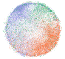
(a) The Pubmed network

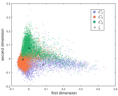
(b) Projected attributes and CRPs

Figure 1: Details of the detection process on Pubmed. (a). The ground truth communities in Pubmed are indicated by node colors. (b). The projected data points of the estimated CRPs and attributes in the ground truth communities $C_{1}$, $C_{2}$ and $C_{3}$. (c). At the second iteration, the conditions in Line 9 of Algorithm 2 are satisfied, and thus $f$ is not updated. (d). The detected communities are shown with node position the same as (a).

​​

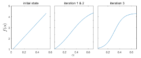
(c) The evolving $f$ along with iterations

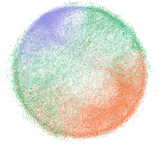
(d) Detected communities in Pubmed

Applying Algorithm 2 to Pubmed, the result at the third iteration shows the largest modularity $Q=0.607$ among $\tau_{max}=10$ iterations, where the corresponding CRPs $\{\bm{\zeta}_{r}|r=1,2,3\}$ and the popularity function $f$ are shown in Fig. 1ab and Fig. 1ac, respectively. From the visualization, we observe that each $\bm{\zeta}$ locates at the position where the attributes in the same community are densely distributed and the distances between different CRPs are relatively large. Therefore, the estimated $\bm{\zeta}$’s are capable to be used as cluster centers of attributes. Starting from the initial state of a linear function (Line 3, Algorithm 2), the node popularity $f$ changes into an $S$-shape curve as the iterations proceed, which is in line with the model selection based on detectability analysis.

For the comparison with ground truth, we present the detected communities in Fig. 1ad. It shows that our method estimates the group memberships of most nodes correctly, while the deviation is mainly caused by the nodes that have nearly the same amount of links to three communities, as shown by the bottom-left of Fig. 1aa and Fig. 1ad. The quantitative evaluation show that our method achieves the best performance compared with the baselines on Pubmed, as will be presented in Section 6.3.

6.3 Comparison with the Baselines

We further qualify the performance of the proposed method by comparing it with the baseline algorithms on various real-life networks with ground truth available. The experimental settings are shown below.

Datasets: Eight real-world network datasets are used in the experiments, including Citeseer, Cora, Pubmed, Facebook, Twitter, Parliament, Arxiv and MAG [9], whose profiles are summarized in Table III. For the datasets, two things need to be noted. First, Facebook and Twitter are two collections of multiple social networks. Following [21, 14, 32], we use the one with largest node size in their collections respectively in the experiments. Second, the node attributes in Pubmed, Arxiv and MAG are real-valued while others are binary-valued. The attributes of Pubmed are converted into binary ones due to the sparsity of the nonzero elements in the literature of SBM-based methods. In contrast, almost all of the node features of Arxiv and MAG are nonzero values.

Baseline algorithms: Four classes of community detection methods are employed for comparison. First, algorithms using graph structure only. To show the importance of fusing attributes in model-based approaches, we adopt the extension of BP inference to DCSBM [24] as a baseline, which can be derived from our algorithm according to Remarks 2 and 4. Besides, the classical Louvain method [50] and CommGAN [51], a recently proposed approach based on deep learning, are compared in the experiments. Second, PGM-based algorithms incorporating both network topology and node attributes. Methods in this class include BAGC [17], CESNA [16], SI [10], BTLSC [14], and CohsMix3 [22]. Third, network embedding approaches that describe the relations among communities, graph structure and node attributes by linear and nonlinear mappings. In this line, NMF-based method ASCD [30] and NEC [31] based on graph neutral networks, are respectively included into comparison. Additionally, in contrast to static optimization algorithms, the methods based on the dynamic process of networked systems are also of interest. To this end, we employ CAMAS [52] as a baseline, which is based on dynamics and the cluster properties in multi-agent systems. Among all the baselines, only NEC can address arbitrary features, while CohsMix3 tackles Gaussian distributed attributes, and others require categorical ones.

The tuning parameters of all the baselines are set according to the authors’ recommendations. For the statistical inference algorithms, we specify the ground-truth value $K^{*}$ for the number of communities to be detected. Specially, there is a ground-truth cluster with only four disconnected nodes in Facebook. On this dataset, we set $K^{*}\in\{8,9\}$ respectively and report the best score. It is worth to note that SI [10] requires all the possible combinations of each dimension of node attributes, which is not scalable to networks in Table III that contain attributes of thousands of dimensions. To solve this problem, we first apply K-Means clustering [48] to the attributes, which converts the high-dimensional feature to univariate one, and then use the clustering result as the input of SI. For CoshMix3 [22] designed for continuous attributes, we conduct PCA on the binary feature vectors of and then take the real-valued attributes in the projection space as the input.

TABLE III: Real-world Dataset Profiles

Class	Dataset	$|V|$	$|E|$	$d$	$K^{*}$	Attribute
Social	Twitter*	171	796	578	6	binary
	Facebook*	1045	26749	576	9	binary
Politics	Parliament	451	5823	108	7	binary
Citation	Citeseer	3312	4732	3703	6	binary
	Cora	2708	5429	1433	7	binary
	Pubmed	19729	44338	500	3	real value
	Arxiv	0.11M	1.3M	128	20	real value
	MAG	0.19M	3.4M	128	9	real value
$K^{*}$: Number of ground-truth communities   $d$: Dimension of attributes
$M$: millions   Facebook*: network id: 107, Twitter*: network id: 629863

Evaluation metrics: We adopt two widely used metrics in community detection to qualify the accordance between experimental results and ground truth and evaluate the competing methods, i.e., Average $F_{1}$ Score (AvgF1) and NMI [53], whose definitions are as follows:

$$\textit{AvgF}1\!=\!\frac{1}{2K^{*}}\!\!\sum_{C^{*}\!\in\mathscr{C}^{*}}\!\max_{C\in\mathscr{C}}\!F_{1}(C^{*}\!,C)+\frac{1}{2K}\!\!\sum_{C\in\mathscr{C}}\!\max_{C^{*}\!\in\mathscr{C}^{*}}\!F_{1}(C\!,C^{*}),$$

$${\!N\!M\!I}=\frac{-2\sum_{p=1}^{K}\sum_{q=1}^{K^{*}}n_{pq}\log\frac{n_{pq}n}{n_{p\cdot}n_{\cdot q}}}{\sum_{p=1}^{K}n_{p\cdot}\log\frac{n_{p\cdot}}{n}+\sum_{q=1}^{K^{*}}n_{\cdot q}\log\frac{n_{\cdot q}}{n}},$$

where $C\in\mathscr{C}$ is a community detected by an algorithm, $C^{*}\!\in\mathscr{C}^{*}$ is a ground-truth community, $K$ is the number of detected communities, $K^{*}$ is that of ground truth, and $F_{1}(C_{p},C_{q})$ is the $F_{1}$ score between two sets $C_{p}$ and $C_{q}$. $n_{pq}=|C_{p}\cap C_{q}|$, $n_{p\cdot}=\sum_{q}n_{pq}$ and $n_{\cdot q}=\sum_{p}{n_{pq}}$. By definition, higher NMI and AvgF1 scores indicate better community divisions.

Note that CAMAS [52] and CESNA [16] may discard anomalous nodes in the detection procedure. Consequently, the NMI index that requires the compared partitions to cover the same node set is unable to evaluate the performances of these two baselines. Instead, we use the extension of NMI named ONMI in [53] for overlapping community detection as the evaluation metric.

TABLE IV: Comparison of the AvgF1 and NMI/ONMI Scores between Our CRSBM and Baselines on Binary Attributed Networks

Network	Twitter*		Facebook*		Cora		Citeseer		Pubmed		Parliament
Metric %	AvgF1	NMI	AvgF1	NMI	AvgF1	NMI	AvgF1	NMI	AvgF1	NMI	AvgF1	NMI
DCSBM	49.33	55.47	38.73	43.23	53.50	36.96	39.17	16.34	55.33	18.14	51.23	41.96
commGAN​	47.63	33.99	32.06	26.79	31.78	6.72	25.03	5.90	41.47	0.11	51.00	20.91
Louvain	37.04	54.64	35.30	55.82	56.42	43.31	41.53	27.74	35.11	17.66	55.78	70.53
BAGC	N/A	N/A	27.67	9.14	36.46	16.97	N/A	N/A	36.33	8.31	29.76	5.27
SI	50.89	54.52	51.61	57.80	49.50	36.08	42.33	28.13	43.17	9.67	43.90	63.53
BTLSC	56.91	66.52	43.54	56.42	46.61	32.04	34.12	15.70	56.91	17.69	62.38	69.74
CohsMix3	27.07	5.56	14.85	10.52	17.74	4.92	19.83	3.38	33.63	0.01	32.49	3.12
NEC	48.80	42.31	44.11	40.21	36.50	55.84*	30.67	27.83*	46.17	4.96	58.14	58.05
ASCD	57.75	66.89	45.13	58.41	51.35	35.56	40.42	24.96	50.83	14.85	66.53	74.77
CRSBM	58.96	59.31	56.77	53.96	57.93	44.42	48.03	29.12	62.98	25.73	72.21	78.65
Metric %	AvgF1	ONMI	AvgF1	ONMI	AvgF1	ONMI	AvgF1	ONMI	AvgF1	ONMI	AvgF1	ONMI
CAMAS	34.02	17.93	31.94	38.42	8.94	0.01	5.80	0.01	8.48	0.01	40.94	34.46
CESNA	43.72	15.53	49.05	27.02	46.14	19.80	3.38	2.26	22.08	1.01	65.64	49.58
CRSBM	58.96	31.15	56.77	32.90	57.93	27.61	48.03	12.25	62.98	19.72	72.21	57.02
* These two results are directly drawn from original paper of NEC [31], while other scores are reported according to our reproduction. Based on our implementation, the NMI on Cora is 20.23%, and that on Citeseer is 13.57%.

The experiments were conducted on the datasets in Table III. We show the results on binary attributed networks (Pubmed included) in Table IV, and those on networks with real-valued attributes in Table VI, respectively, where the best scores for each network are highlighted in bold and N/A means that the algorithm only detected one trivial community on the network. The experiments of NEC and commGAN were conducted on a NVIDIA RTX3090 GPU with 24GB GPU memory and others on a PC with Intel i9-10900X@3.7 GHz CPU and 128GB memory.

TABLE V: Comparison of Clustering Accuracy on Twitter* and Facebook*

Method	SI	BTLSC	ASCD	CRSBM
Twitter*	0.4528	0.6288	0.5682	0.5814
Facebook*	0.3292	0.6548	0.4745	0.7042

From Table IV, we observe that: First, our CRSBM is the only attributed community detection method that is superior to DCSBM on all the eight datasets, which shows that CRSBM can effectively fuse attributes to improve the performance of detection. Second, CRSBM, BTLSC, SI, ASCD and NEC are effective on both dense and sparse networks, while CohsMix3, CAMAS and CESNA show inferior performances on the networks that have a small average node degree around $4$. Third, our method significantly outperforms the baselines on Citeseer, Pubmed, and Parliament. And our results on Cora show the best score in terms of AvgF1 and the second best in terms of NMI.

It is noticed that the ranks of competitors given by NMI and AvgF1 have remarkable difference on Twitter* and Facebook*. In order to make the comparison more convincing, we additionally compare the clustering accuracy ($AC$) scores of SI, BTLSC, ASCD and our CRSBM on these two datasets, which are displayed in Table V. The clustering accuracy is defined as

$$AC(C,C^{*})=\frac{1}{n}\sum\nolimits_{i=1}^{n}\delta(C^{*}_{i},map(C_{i})),$$

where $map(\cdot)$ is the permutation that maps each label $C_{i}$ to the equivalent label from the dataset. It is shown in Table V that CRSBM gives the highest accuracy on Facebook* and the second highest score on Twitter* only after BTLSC, while the accuracies of SI are the lowest on both datasets. Taking the three metrics together, CRSBM achieves the best scores in terms of two on Facebook* and shows a competitive performance on Twitter*.

TABLE VI: Comparison between Baselines and CRSBM on Networks with Real-valued Node Attributes

Network	Arxiv		MAG
Metric %	AvgF1	NMI	AvgF1	NMI
DCSBM	17.85	19.16	25.07	24.62
Louvain	22.24	24.90	27.38	28.01
commGAN	21.73	11.38	30.33	20.93
CohsMix3	Out of Memory		Out of Memory
NEC	Out of Memory		Out of Memory
CRSBM	26.08	24.95	38.83	32.13

Finally, we report the experimental results on large networks. As indicated in Table VI, CRSBM beats the baselines on two large networks. For these datasets, CoshMix3 and NEC ran out of the memory of our device because of their $O(n^{2})$ space complexity. In contrast, our method only consumes $O(qm)$ space and thus can be applied to large-scale sparse networks. Overall, our method achieves the best performance among the competing approaches. Moreover, compared to other algorithms, CRSBM also shows better applicability to various node attributed networks, whose edges may be sparse or dense, and node attributes may be categorical or real-valued.

6.4 Comparison of Time Efficiency

For a clear comparison on time efficiency, we first present the time complexity of the employed competing methods in Table VII. It shows that our algorithm has a competitive theoretical time efficiency compared to other baselines. To validate this, we report the CPU times of the attributed community detection algorithms in Fig. 2. It is noted that the GPU times of NEC are not included, because the main limit of the scalability of NEC is the memory usage. We also compare the increase of CPU times (histograms) with that of the number of edges (blue stairs) on different datasets to show the time scalability. As displayed in Fig. 2, CRSBM not only demonstrates the best time efficiency compared to the baselines, but also has a good time scalability on large networks with millions of edges.

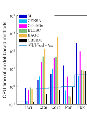
Figure 2: CPU times in seconds of the model-based algorithms. The CPU times are shown by histograms, and the comparison between the increase of edge sizes and that of CPU time is shown by blue stairs, where $|E|$ is the edge size of the dataset, $|E_{twi}|$ is that of Twitter, and $t_{twi}$ is the CPU time of our CRSBM on Twitter*. Twi: Twitter, Par: Parliament, Cite: Citeseer, Fbk: Facebook*, Pub: Pubmed. Implementation: CRSBM, SI, CESNA in C/C++; BAGC, BTLSC in Matlab; CohsMix3 in R.

TABLE VII: Comparison of the Time Complexity between Our CRSBM and Attributed Community Detection Baselines

Methods	CRSBM	BAGC	SI	BTLSC	CohsMix3	CESNA	NEC	CAMAS
Time complexity	$O(q^{2}m+qnd)$	$O(q^{2}n^{2})$	$O(q^{2}m+2^{d})$	$O(q^{2}n^{2}+nd)$	$O(qn^{2}d)$	$O(m+qn)$	$O(n^{2}+qn)$	$O(n^{2})$

7 Conclusion

In this paper, we have proposed a novel PGM named CRSBM for attributed community detection without any requirements on the distribution of attributes, which can be either categorical or real-valued. This mainly contributes to the incorporation of the distances between attributes in the model. In detail, we have first described the impact of attributes on node popularity by attaching a function of the distances to the classical SBM. Then to choose an appropriate node popularity function, which inherently relates to the model selection problem, we analyzed the detectability of communities for CRSBM. And it came out that a function showing an $S$-shape curve is a good choice to describe the popularity, as well as the weight of different attributes in data fusion. After that, an efficient algorithm was developed to estimate the parameters and detect the communities. Extensive experiments on real-world networks has shown that our method is superior to the competing approaches.

For quantitative analysis, we have derived the detectability condition for CRSBM, which has been verified by numerical experiments on artificial networks. As a quantification of the effect of node attributes on community detection, the detectability shows that if there are multiple (but not all) communities with all their nodes containing the same categorical attribute, the detectability can still be improved compared to that with attributes being ignored, where the improvement is mainly determined by the average node degree as well as the level of the dependence on attributes.

In the future, we plan to apply our detectability-based model selection scheme to other methods for the comparison and choice of various a priori models and parameters.

Proof of Theorem 1: For any two matrices $T^{i}$ and $T^{j}$ defined in (20), it follows that $T^{i}=T^{j}$ if $\varsigma_{i}=\varsigma_{j}$, that is, $i$ and $j$ have the same categorical attribute. Otherwise, let $z_{i}=r$ and $z_{j}=s$, $T^{i}$ can be transformed into $T^{j}$ by first swapping its $r$th and $s$th rows and then swapping the $r$th and $s$th columns, which are elementary transformations. Therefore, the matrices $\{T^{i}|i\in V\}$ are similar to each other, and share the same eigenvalues.

Note that $\sum_{r=1}^{q^{*}}\psi^{i}_{r}=1$, which yields $\mathbf{1}^{\mathrm{T}}(I-\bm{\psi}^{i}\mathbf{1}^{\mathrm{T}})=\mathbf{0}^{\mathrm{T}}$. Then it follows that $\mathbf{1}^{\mathrm{T}}T^{i}=\mathbf{0}^{\mathrm{T}}=0\mathbf{1}^{\mathrm{T}}$. Thus, $0$ is an eigenvalue of $T^{i}$. Before solving for other eigenvalues of $T^{i}$, we first present some notations. Let $\mathbf{v}_{rs}\triangleq(0,\ldots,1,0\ldots,-1,\ldots,0)^{\mathrm{T}}$, where $1$ is the $r$th and $-1$ is the $s$th entry, $r\neq s$, while other entries are all $0$. We also define an auxiliary matrix $\tilde{T}^{i}\triangleq\tilde{D}^{-1}\Psi^{i}~{}\!\Omega~{}\!F^{i}$, which satisfies that $T^{i}\mathbf{v}_{rs}=\tilde{T}^{i}\mathbf{v}_{rs}$.

Without loss of generality, let $z_{i}=r=1$, then $F^{i}=\text{diag}(1,\ldots,1,\gamma,\ldots,\gamma)$ with $1$’s being the first $q_{b}$ entries, and $\bm{\psi}^{i}\propto(\gamma,1,\ldots,1)$ with $\gamma$ the first entry. After some lines of linear algebra, we obtain that $\mathbf{v}_{1s},s=2,\ldots,{q}_{b}$ are $q_{b}-1$ eigenvectors of $\tilde{T}^{i}$ with the corresponding eigenvalues sharing the same value

$$\lambda_{1s}(\tilde{T}^{i})=\frac{\omega_{in}-\omega_{out}}{\omega_{in}\!+\!(q^{*}\!+\!1\!-\!q_{b})\gamma\omega_{out}\!+\!(q_{b}-1)\omega_{out}}.$$ (38)

Similarly, setting $r=q_{b}+1$, we obtain that $\mathbf{v}_{rs},s\!=\!r\!+\!1,\ldots,q^{*}$ are $q^{*}-q_{b}+1$ eigenvectors of with the corresponding eigenvalues sharing the same value

$$\lambda_{q_{b}+1,s}(\tilde{T}^{i})\!=\!\frac{\omega_{in}-\omega_{out}}{\omega_{in}\!+\!(q^{*}\!-\!1\!-\!q_{b})\omega_{out}\!+\!q_{b}\gamma^{-1}\omega_{out}}.$$ (39)

Given that $T^{i}\mathbf{v}_{rs}=\tilde{T}^{i}\mathbf{v}_{rs}$, the values in (38) and (39) are also eigenvalues of $T^{i}$. Now we have found $q^{*}-1$ real eigenvalues of $T^{i}$. All the $q^{*}$ eigenvalues of $T^{i}$ are real since the complex eigenvalues must be conjugate. The remaining one, denoted by $\lambda_{last}(T^{i})$, can be computed according to the fact that $\sum_{k}\lambda_{k}(T^{i})=\text{trace}(T^{i})$, where $\text{trace}(T^{i})=\sum_{r}T^{i}_{rr}$ is the trace of $T^{i}$. Given that $\gamma>1$ and $\omega_{in}>\omega_{out}$, we have $\lambda_{q_{b}+1,s}(T^{i})>\lambda_{1s}(T^{i})>0$, and by direct computation we also find that $\lambda_{last}(T^{i})<\lambda_{q_{b}+1,s}(T^{i})$. Therefore, $\lambda_{q_{b}+1,s}(T^{i})$ in (39) is the largest eigenvalue among all the $q^{*}$ real eigenvalues of $T^{i}$, $\forall i\in V$. This completes the proof.

Ren Ren received the B.S. degree from the School of Mathematical Sciences, University of Electronic Science and Technology of China, Chengdu, in 2019. He is currently pursuing the M.S. degree in School of Automation Engineering, University of Electronic Science and Technology of China. His current research interests include network analysis and unsupervised learning.

Jinliang Shao received the B.Sc. and Ph.D. degrees from the University of Electronic Science and Technology of China (UESTC), Chengdu, in 2003 and 2009, respectively. During 2014, he was a visiting scholar in Australian National University, Australia, and during 2018, he was a visiting scholar in Western Sydney University, Australia. He is currently an associate professor in the School of Automation Engineering, UESTC. His research interests include multi-agent system, robust control, and matrix analysis with applications in control theory.

Adrian N. Bishop has held academic positions at the Royal Institute of Technology (KTH) in Stockholm, at the Australian National University (ANU) in Canberra and at the University of Technology Sydney (UTS) in Sydney. He is also a Research Scientist at NICTA in Canberra and Sydney. He is funded by an ARC Discovery Early Career Research Award (DECRA) Fellowship, NICTA and the US Air Force among other funding bodies. His current research interests fall within the intersection of statistical control and estimation, statistical machine learning and distributed (or large-scale) applicability of such topics.

Wei Xing Zheng (M’93-SM’98-F’14) received the B.Sc. degree in Applied Mathematics, the M.Sc. degree and the Ph.D. degree in Electrical Engineering from Southeast University, Nanjing, China, in 1982, 1984, and 1989, respectively. He is currently a University Distinguished Professor with Western Sydney University, Sydney, Australia. Over the years he has also held various faculty/research/visiting positions at several universities in China, UK, Australia, Germany, USA, etc. He has been an Associate Editor of several flagship journals, including IEEE Transactions on Automatic Control, IEEE Transactions on Cybernetics, IEEE Transactions on Neural Networks and Learning Systems, IEEE Transactions on Control of Network Systems, IEEE Transactions on Circuits and Systems-I: Regular Papers and so on. He is a Fellow of IEEE.

References

- [1] J. Yang and J. Leskovec, “Defining and evaluating network communities based on ground-truth,” Knowl. and Info. Sys., vol. 42, no. 1, pp. 181–213, 2015.
- [2] S. Fortunato and D. Hric, “Community detection in networks: A user guide,” Phys. Rep., vol. 659, pp. 1–44, 2016.
- [3] M. E. Newman, “Modularity and community structure in networks,” Proc. Natl. Acad. Sci., vol. 103, no. 23, pp. 8577–8582, 2006.
- [4] M. E. Newman, “Network structure from rich but noisy data,” Nat. Phys., vol. 14, no. 6, pp. 542–545, 2018.
- [5] D. Hric, R. K. Darst, and S. Fortunato, “Community detection in networks: Structural communities versus ground truth,” Phys. Rev. E, vol. 90, no. 6, p. 062805, 2014.
- [6] A. Decelle, F. Krzakala, C. Moore, and L. Zdeborová, Asymptotic analysis of the stochastic block model for modular networks and its algorithmic applications, Phys. Rev. E, vol. 84, no. 6, p. 066106, 2011.
- [7] C. Moore, The Computer Science and Physics of Community Detection: Landscapes, Phase Transitions, and Hardness, Arxiv preprint 1702.00467, Feb. 2017.
- [8] P. Chunaev, “Community detection in node-attributed social networks: a survey,” Computer Science Review, vol. 37, p. 100286. 2020.
- [9] K. Wang, Z. Shen, C. Huang, C.-H. Wu, Y. Dong, and A. Kanakia, “Microsoft Academic Graph: When experts are not enough,” Quant. Sci. Stud., vol. 1, no. 1, pp. 396–413, Feb. 2020.
- [10] M. E. J. Newman and A. Clauset, ”Structure and inference in annotated networks, Nat. Commun.,” vol. 7, no. 1, p. 11863, 2016.
- [11] D. Hric, T. P. Peixoto, and S. Fortunato, “Network structure, metadata, and the prediction of missing nodes and annotations,” Phys. Rev. X, vol. 6, no. 3, pp. 1–15, 2016.
- [12] L. Peel, D. B. Larremore, and A. Clauset, “The ground truth about metadata and community detection in networks,” Sci. Adv., vol 3, no.5, p. e1602548, May 2017.
- [13] P. Zhang, C. Moore, and L. Zdeborová, “Phase transitions in semisupervised clustering of sparse networks,” Phys. Rev. E, vol. 90, no. 5, p. 052802, 2014.
- [14] D. Jin et al., ”Detecting Communities with Multiplex Semantics by Distinguishing Background, General, and Specialized Topics,” in IEEE Trans. on Knowl. and Data Eng., vol. 32, no. 11, pp. 2144-2158, Nov. 2020.
- [15] P. W. Holland, K. B. Laskey, and S. Leinhardt, “Stochastic blockmodels: First steps,” Soc. Networks, vol. 5, no. 2, pp. 109–137, 1983.
- [16] J. Yang, J. McAuley, and J. Leskovec, “Community detection in networks with node attributes,” in Proc. - IEEE Int. Conf. Data Mining, ICDM, 2013, pp. 1151–1156.
- [17] Z. Xu, Y. Ke, Y. Wang, H. Cheng, and J. Cheng, ”A model-based approach to attributed graph clustering,” in Proc. 2012 Int. Conf. Manag. Data - SIGMOD ’12, New York, USA: ACM Press, 2012, p. 505.
- [18] L. Hu, K. C. C. Chan, X. Yuan and S. Xiong, ”A Variational Bayesian Framework for Cluster Analysis in a Complex Network,” in IEEE Trans. on Knowl. and Data Eng., vol. 32, no. 11, pp. 2115-2128, 1 Nov. 2020.
- [19] Tiago P. Peixoto, Descriptive vs. inferential community detection: pitfalls, myths and half-truths, Arxiv preprint 2112.00183, Dec. 2021.
- [20] M. Gerlach, T. P. Peixoto, and E. G. Altmann,“A network approach to topic models,” Sci. Adv., vol. 4, no. 7, Jul. 2018.
- [21] D. He, Z. Feng, D. Jin, X. Wang, and W. Zhang, “Joint identification of network communities and semantics via integrative modeling of network topologies and node contents,” 31st AAAI Conf. Artif. Intell. 2017.
- [22] H. Zanghi, S. Volant, and C. Ambroise, “Clustering based on random graph model embedding vertex features,” Pattern Recognit. Lett., vol. 31, no. 9, pp. 830–836. 2010.
- [23] T. P. Peixoto, “Hierarchical Block Structures and High-Resolution Model Selection in Large Networks,” Phys. Rev. X, vol. 4, no. 1, p. 011047, 2014.
- [24] X. Yan et al. “Model selection for degree-corrected block models,” J. Stat. Mech. Theory Exp., vol. 2014, no. 5, P05007, 2014.
- [25] Z. Xu, J. Cheng, X. Xiao, R. Fujimaki, and Y. Muraoka, “Efficient nonparametric and asymptotic Bayesian model selection methods for attributed graph clustering,” Knowl. Inf. Syst., vol. 53, no. 1, pp. 239–268, Oct. 2017.
- [26] B. Karrer and M. E. J. Newman, “Stochastic blockmodels and community structure in networks,” Phys. Rev. E, vol. 83, no. 1 pp. 1–11, 2011.
- [27] M. E. J. Newman, “Equivalence between modularity optimization and maximum likelihood methods for community detection,” Phys. Rev. E, vol. 94, no. 5, p. 052315, Nov. 2016.
- [28] T.P. Peixoto, “Bayesian Stochastic Blockmodeling,” in Advances in Network Clustering and Blockmodeling. Wiley, pp. 289–332, 2019.
- [29] X. Wang, D. Jin, X. Cao, L. Yang, and W. Zhang, “Semantic community identification in large attribute networks,” in 31st AAAI Conf. Artif. Intell. 2016.
- [30] M. Qin, D. Jin, K. Lei, B. Gabrys, and K. Musial-Gabrys, “Adaptive community detection incorporating topology and content in social networks,” Knowledge-Based Syst., vol. 161, pp. 342–356, Dec. 2018.
- [31] H. Sun et al., “Network Embedding for Community Detection in Attributed Networks,” ACM Trans. Knowl. Discov. Data, vol. 14, no. 3, pp. 1–25, May 2020.
- [32] Y. Li, C. Sha, X. Huang, and Y. Zhang, ”Community detection in attributed graphs: An embedding approach.” in 32nd AAAI Conf. Artif. Intell. 2018.
- [33] L. Liao, X. He, H. Zhang and T. Chua, “Attributed Social Network Embedding,” in IEEE Trans. on Knowl. and Data Eng., vol. 30, no. 12, pp. 2257-2270, Dec. 2018.
- [34] Z. Chen, A. Sun, and X. Xiao, “Incremental Community Detection on Large Complex Attributed Network,” ACM Trans. Knowl. Discov. Data, vol. 15, no. 6, pp. 1–20, May 2021.
- [35] A. Faqeeh, S. Osat, and F. Radicchi, “Characterizing the Analogy Between Hyperbolic Embedding and Community Structure of Complex Networks,” Phys. Rev. Lett., vol. 121, no. 9 p. 09830, 2018.
- [36] F. Simini, M. C. González, A. Maritan, and A.-L. Barabási, “A universal model for mobility and migration patterns,” Nature, vol. 484, no. 7392, pp. 96–100, 2012.
- [37] M. Steinbach, V. Kumar, and P. Tan, Cluster analysis: basic concepts and algorithms,in Introduction to data mining, 1st edition. Pearson Addison Wesley, 2005.
- [38] M. Mezard and A. Montanari, Information, Physics, and Computation. USA: Oxford University Press, Inc., 2009.
- [39] P. Zhang and C. Moore, “Scalable detection of statistically significant communities and hierarchies, using message passing for modularity,” Proc. Natl. Acad. Sci., vol. 111, no. 51, pp. 18 144–18 149, 2014.
- [40] A. L. Madsen, “Belief update in clg bayesian networks with lazy propagation,” Int. J. Approx. Reason., vol. 49, no. 2, pp. 503–521, 2008.
- [41] W. Gatterbauer, S. Gunnemann, D. Koutra, and C. Faloutsos, “Linearized and single-pass belief propagation,” Proc. VLDB Endow., vol. 8, no. 5, pp. 581–592, Jan. 2015.
- [42] D. Eswaran, S. Gunnemann, C. Faloutsos, D. Makhija, and M. Kumar, “ZooBP: Belief Propagation for Heterogeneous Networks,” Proc. VLDB Endow., vol. 10, no. 5, pp. 625–636, Jan. 2017.
- [43] F. Krzakala, C. Moore, E. Mossel, J. Neeman, A. Sly, L. Zdeborova, and P. Zhang, “Spectral redemption in clustering sparse networks, ” Proc. Natl. Acad. Sci., vol. 110, no. 52, pp. 20935–20940, 2013.
- [44] E. Mossel, J. Neeman, and A. Sly, ”A Proof of the Block Model Threshold Conjecture,” Combinatorica, vol. 38, no. 3, pp. 665–708, 2018.
- [45] J. Banks, C. Moore, J. Neeman, and P. Netrapalli, “Information-theoretic thresholds for community detection in sparse networks,” in Conf. on Learning Theory, pp. 383–416, 2016.
- [46] H. Kesten and B. P. Stigum, “Additional Limit Theorems for Indecomposable Multidimensional Galton-Watson Processes,” Ann. Math. Stat., vol. 37, no. 6, pp. 1463–1481, 1966.
- [47] F. Radicchi et al. ”Defining and identifying communities in networks,” Proc. Natl. Acad. Sci., vol. 101, no. 9, pp. 2658–2663, 2004.
- [48] A. David, “K-means++: The advantages of careful seeding,” in 18th annual ACM-SIAM symposium on Discrete algorithms (SODA), New Orleans, Louisiana, 2007, pp. 1027–1035.
- [49] H. Abdi and L. J. Williams, “Principal component analysis,” Wiley Interdisciplinary Rev. Comput. Stat., vol. 2, no. 4, pp. 433–459, 2010.
- [50] V. D. Blondel, J.-L. Guillaume, R. Lambiotte, and E. Lefebvre, “Fast unfolding of communities in large networks,” J. Stat. Mech. Theory Exp., vol. 2008, no. 10, p. P10008, Oct. 2008.
- [51] Y. Jia, Q. Zhang, W. Zhang, and X. Wang, “CommunityGAN: Community Detection with Generative Adversarial Nets,” in The World Wide Web Conference, May 2019, pp. 784–794.
- [52] Z. Bu, G. Gao, H.-J. Li, and J. Cao, “CAMAS: A cluster-aware multiagent system for attributed graph clustering,” Inf. Fusion, vol. 37, pp. 10–21, 2017.
- [53] A. Lancichinetti, S. Fortunato, and J. Kertész, “Detecting overlapping and hierarchical community structure in complex networks,” New J. Phys., vol. 11, no. 3, p. 033015, 2009.