Pixel domain multi-resolution minimum variance painting of CMB maps

Abstract

This work introduces an unbiased minimum variance painting of the pixel domain CMB maps for both the missing and available sky regions. In the missing region, it generates CMB realizations that have identical statistical properties to the expected CMB signal; and in the available region, it significantly alleviate the unwanted residuals, e.g., the residual of EB-leakage. The time cost of this method follows $\sim$$O(N_{side}^{3})$ ($N_{side}$ is the map resolution parameter), which is similar to the fast spherical harmonic transforms and is much better than the traditional minimum variance method that follows $\sim$$O(N_{side}^{6})$. This method is the basis of a series of minimum variance estimations for analyzing CMB datasets, and more works based on it will follow in the future.

1 Introduction

In the measurement of cosmic microwave background (CMB) anisotropy, a few key problems were constantly studied from the beginning until the present day. For example, how to compute the full sky CMB angular power spectrum (APS) from various cosmological models and vice versa; and how to estimate the true CMB signal and APS from incomplete and contaminated sky maps. In this work, we focus on the latter, especially the estimation and reconstruction of pixel domain CMB signals, because it usually makes following CMB analysis much easier.

For the case of CMB temperature, the best unbiased solution of this kind of problem was given by [1], which is usually referred to as the fisher estimator, a method that finds the CMB APS with the maximum likelihood condition. It was also mentioned in [1], that the maximum likelihood and minimum variance conditions are equivalent for the Gaussian isotropic CMB signal; thus, one is free to start from either side.

The main problem of the fisher estimator is the computational cost. According to the tests in [2], a full implementation of the fisher estimator at a relatively low resolution ($N_{side}=64$) of the HEALPix pixelization scheme [3] already requires about $4\times 10^{5}$ CPU hours and 19 TB memory, which is a heavy task even for a super cluster. For higher resolutions, the time cost scales as $O(N_{side}^{6})$; thus, the computation is essentially impossible. Therefore, many alternative methods were developed. Some of them keep pursuing the maximum likelihood (or minimum variance), but manage to do the job in a faster way ([4, 5, 6, 7, 8, 9, 10], and a review can be found in section 5 of [11]); and some others choose to accept sub-optimal results, but as an exchange, the time cost can be significantly reduced, e.g., the pseudo-$C_{\ell}$ method [12, 13] and the Spice estimator [14]. Overall speaking, the former still requires to use a super cluster, especially for the case of higher resolutions or higher-$\ell$s; and the latter is the currently most practical way to estimate the high-$\ell$ CMB APS, but the quality of the result is relatively lower, and especially, it cannot deal with a pixel-domain estimation.

For the case of polarization, a key problem that hinders the minimum variance solution is the leakage from the E-mode polarizations to the B-mode polarizations, called the EB-leakage [15, 16]. However, in our recent work [17], it was shown how to explicitly correct the EB-leakage in the pixel domain, and with some clearly defined preconditions, the results are proven to be the best ones. Thus, it is about time to design a series of minimum variance solution for both the temperature and polarization, and from map to the final cosmological parameters. Given the solution of EB-leakage, the most urgent problem at the moment is to greatly reduce the computational cost of the pixel domain minimum variance estimation, which is the basis of all following works in this series, and will be the main goal of this work.

Meanwhile, by greatly reducing the time cost of pixel domain minimum variance estimation, several interesting possibilities are also turned on, especially for studying the large-scale and low-$\ell$ problems. For example, it will become possible to change the sky mask pixel-by-pixel to investigate the impact upon all kinds of large scale anomalies, in order to find out a possible association to a specific sky region.

The outline of this work is as follows: In section 2, we explain some mathematical basis of the method, and the technical details of implementation are introduced in section 3. The implementation and performance are tested and illustrated in section 4, and a conclusion and discussion is given in section 5.

2 The mathematical basis

The multi-resolution minimum variance painting (MrMVP) is based on the ideal of constrained in-painting by [18], but some similar ideas can also be found in [19, 20, 21]. Basically, assume we have an available dataset $\bm{X}=\bm{S}+\bm{N}$, where $\bm{S}$ is the true signal and $\bm{N}$ is the noise. For convenience, here $\bm{N}$ includes all unwanted components like the noise, systematics and various residuals. The main goal of painting is to estimate $\bm{S}$ from $\bm{X}$ in both the missing and available regions, including the expectation and constrained realizations. Customarily, when we focus on the reconstruction of the missing region, the operation is called an in-painting.

A basic in-painting method only focus on estimating the expectation in the missing region, like the diffusive in-paint method [22, 23]; whereas a complete in-painting method will consider the expectation and constrained realizations at the same time, like the one in [18]. With the well known theory of multi-variant minimum variance regression (for example, see appendix A of [17]), if we only want to solve for the expectation, then the result is given by the following unbiased minimum variance solution:

$$\bm{\widetilde{S}} = \bm{PQ}^{-1}\bm{X},$$ (2.1)

where $\bm{\widetilde{S}}$ is the pixel domain expectation of $\bm{S}$ and $\bm{P}=\langle\bm{XS}^{T}\rangle$, $\bm{Q}=\langle\bm{XX}^{T}\rangle$ are the covariance matrices of $\bm{X}$-with-$\bm{S}$ and $\bm{X}$-with-$\bm{X}$, respectively. If we further assume $\bm{S}$ and $\bm{N}$ are uncorrelated (which is usually true), then the above equation becomes

$$\bm{P}=\langle\bm{SS}^{T}\rangle,~{}~{}\bm{Q}=\langle\bm{SS}^{T}\rangle+\langle\bm{NN}^{T}\rangle,$$ (2.2)

and eq. (2.1) becomes the well known Wiener filter. Note that in eq. (2.1), if we are dealing with the missing region, then $\bm{X}$ and $\bm{S}$ belong to different regions, but $\bm{P}$ is not zero, which makes the estimation of the missing region possible.

It is important to emphasis that $\bm{\widetilde{S}}$ is an “expectation” but not a “realization”; such that the true signal $\bm{S}$ is always different to $\bm{\widetilde{S}}$. In fact, in the view of statistics, the true signal $\bm{S}$ is included as a member of the ensemble $\{\bm{S}_{i}\}$ containing all possible realizations, and $\bm{S}$ is not superior compared to any other members. Therefore, the next immediate question is how to generate the constrained ensemble $\{\bm{S}_{i}\}$, which is important because $\bm{S}_{i}$, as fullsky realizations of the CMB signal, make many estimations extremely convenient, as also mentioned in [18].

The generation of ensemble $\{\bm{S}_{i}\}$ is based on the following constraint and prior conditions:

1. Constraint: $\bm{S}_{i}$ has to be consistent with the actual dataset $\bm{X}$.

2. Prior condition: In case of CMB, $\bm{S}_{i}$ should be Gaussian and isotropic.

3. Prior condition: $\bm{P}$ and $\bm{Q}$ are determined either by the prior APS or by an iterative solution.

With the above constraint and prior conditions, the ensemble $\{\bm{S}_{i}\}$ can be generated from the key equation provided in [24, 18]. For convenience of reading, it is retyped below using the above notations:

$$\bm{S}_{i}=\bm{\widetilde{S}}+\bm{s}_{i}-\bm{PQ}^{-1}\bm{x}_{i},$$ (2.3)

where $\bm{S}_{i}$ is a constrained realization; $\bm{s}_{i}$ is the $i$-th unconstrained fullsky realization generated with the prior conditions 2–3, $\bm{x}_{i}$ is $\bm{s}_{i}$ plus noise, and $\bm{\widetilde{S}}$ is the expectation given by 2.1 that carries the constraint 1. The physical meaning of the above equation is: a properly constrained realization is the expectation $\bm{\widetilde{S}}$ solved from the real data, plus the difference between an unconstrained realization $\bm{s}_{i}$ and the expectation $\bm{PQ}^{-1}\bm{x}_{i}$ solved from $\bm{s}_{i}$.

As explained in [1], the CMB statistical properties are fully described by its covariance matrix; thus, in order to prove $\bm{S}_{i}$ is a properly constrained CMB realization, we need to show that it has the same covariance matrix with the expected CMB signal, i.e., it is statistically indistinguishable with a true CMB signal. The mathematical proof of this point is given as follows: With eq. (2.3), the covariance matrix of $\bm{S}_{i}$ is

$$\langle\bm{S}_{i}\bm{S}_{i}^{t}\rangle= \langle(\bm{\widetilde{S}}+\bm{s}_{i}-\bm{M}\bm{x}_{i})\cdot(\bm{\widetilde{S}}+\bm{s}_{i}-\bm{M}\bm{x}_{i})^{t}\rangle$$ (2.4)

$$= \langle\bm{\widetilde{S}}\bm{\widetilde{S}}^{t}\rangle+\langle\bm{s}_{i}\bm{s}_{i}^{t}\rangle+\bm{M}\langle\bm{x}_{i}\bm{x}_{i}^{t}\rangle\bm{M}^{t}-\bm{M}\langle\bm{x}_{i}\bm{s}_{i}^{t}\rangle-\langle\bm{s}_{i}\bm{x}_{i}^{t}\rangle\bm{M}^{t}$$

$$= \bm{M}\bm{Q}\bm{M}^{t}+\bm{P}+\bm{M}\bm{Q}\bm{M}^{t}-\bm{M}\bm{P}-\bm{P}\bm{M}^{t}$$

$$= \bm{P}+2\bm{M}\bm{Q}\bm{M}^{t}-\bm{M}\bm{P}-\bm{P}\bm{M}^{t}$$

$$= \bm{P}+2\bm{P}\bm{Q}^{-1}\bm{Q}\bm{Q}^{-1}\bm{P}-2\bm{P}\bm{Q}^{-1}\bm{P}$$

$$= \bm{P}.$$

Therefore, the constrained realizations $\bm{S}_{i}$ have identical statistical properties with the true CMB signal, and is hence a properly constrained fullsky CMB realization. Moreover, because the CMB angular power spectrum is completely determined by the pixel domain covariance matrix, we automatically get the conclusion that, the expected angular power of $\bm{S}_{i}$ is also identical to the expected CMB angular power spectrum. Therefore, eq. (2.3) is enough to establish the mathematical basis of MrMVP for both the pixel and harmonic domains, and the rest of the problem is about the multi-resolution scheme and details of implementation, which will be described in the next section.

3 Implementation and technical details

In this section, we describe some technical details of the implementation of MrMVP.

3.1 Fast computation of the pixel domain covariance matrix

The implementation of eq. (2.3) depends on computing the pixel-domain covariance matrices $\bm{P}$ and $\bm{Q}$ that are consist of the CMB and non-CMB parts. Using the non-polarized case for illustration, the CMB part of the covariance matrix is given by the following equation:

$$C_{ij}=\frac{1}{4\pi}\sum_{\ell}{(2l+1)W_{\ell}^{2}C_{\ell}P_{\ell}[\cos{(\theta_{ij})}]},$$ (3.1)

where $C_{ij}$ is the element of the CMB covariance matrix, $C_{\ell}$ is the CMB APS, $W_{\ell}$ is the transfer function, $P_{\ell}(x)$ is the Legendre polynomial, and $\theta_{ij}$ is the open angle between the $i$-th and $j$-th pixels. Let’s take $N_{side}=512$ as an example: At this resolution, there are about $3\times 10^{6}$ pixels on the sky, and we usually go up to $\ell_{max}=1536$. Thus there are about $10^{13}$ elements in the covariance matrix, and the number of float point operations is at the order of $10^{16}$. Although eq. (3.1) is not very complicated, such a big number of operations should still be avoided.

In this work, the idea is to first greatly oversample $\theta_{ij}$ from 0 to $\pi$. In the HEALPix pixelization scheme, at a resolution of $N_{side}$, $4N_{side}$ points between 0 and $2\pi$ are usually enough to support the spherical harmonic transforms, but we oversample it to $64N_{side}$ points to compute the function $C(\theta)$, which is more than enough to guarantee the precision. Then the full covariance matrix is computed by linear interpolation of the oversampled $C(\theta)$ function. By this way, the time cost is reduced from $aN_{pix}^{3}$ to $bN_{pix}^{2}$. Note that not only the power index is reduced from 3 to 2, but also the constant coefficient $b$ is much smaller than $a$, because it is much easier to compute the interpolation than to compute the Legendre polynomials.

In case of the polarization, the full pixel domain covariance matrices are given in eq. (10) of [25] or eq. (A10-A15) of  [26], and they are also in form of $C(\theta)$; thus, the computation can be accelerated with the same technique.

3.2 The degree-of-freedom problem

According to eq. (2.1), we need to invert the covariance matrix $\bm{Q}$ to get the solution, thus we want $\bm{Q}$ to be non-singular. For convenience of discussion, $\bm{Q}$ is converted to the harmonic domain: If the CMB signal is Gaussian and isotropic, then a full covariance matrix of the CMB in the harmonic domain is diagonal and takes the following look:

$$\bm{C}=\begin{pmatrix}C_{0}&0&0&0&0&\cdots\\ 0&C_{1}&0&0&0&\cdots\\ 0&0&C_{1}&0&0&\cdots\\ 0&0&0&C_{1}&0&\cdots\\ 0&0&0&0&C_{2}&\cdots\\ \cdots&\cdots&\cdots&\cdots&\cdots&\cdots\end{pmatrix},$$ (3.2)

where each $C_{\ell}$ appears $2\ell+1$ times. Thus for a finite $\ell_{max}$, the maximum number of non-zero diagonal elements is $(\ell_{max}+1)^{2}$, which is equal to the matrix’s upper limit of degree-of-freedom (DOF).

However, the size of the covariance matrix is determined not by $\ell_{max}$, but by the number of map pixels. With the HEALPix pixelization scheme, this number is equal to $12N_{side}^{2}$, where $N_{side}=2,4,8,\cdots$ is the resolution parameter. Therefore, to ensure that $\bm{Q}$ have enough DOF and is hence non-singular, the following inequality must be satisfied:

$$(\ell_{max}+1)^{2}\geq 12N_{side}^{2}\Longrightarrow\ell_{max}\geq\sqrt{12}N_{side}-1\approx 3.5N_{side}.$$ (3.3)

However, according to the HEALPix manual, the pixelization scheme by HEALPix can only support a computation up to $\ell_{max}=3N_{side}-1$. Higher $\ell$s can still be computed but are no longer reliable. Thus we have a gap between $3N_{side}$ and $3.5N_{side}$, which can make $\bm{Q}$ singular. Because of this degree of freedom problem, it is actually impossible to do a pixel domain minimum variance estimation at the original resolution without prior information — it has to be done either with a prior APS or by combining two neighboring resolutions.

In principle, both ways are allowed: If we use a prior APS, then the analysis becomes a typical Bayesian estimation and can be further developed into a suit of minimum variance estimations from map to cosmological parameters. This is our goal in the following works; however, if we choose to combine two neighboring resolutions, then the estimation is done in a bind way, which helps to make the result more robust by providing a crosscheck free from the prior APS. In this work, we are mainly dealing with the pixel domain estimation; thus, we shall focus on the latter.

3.3 The transfer function of downgrading/upgrading

In order to do the minimum variance estimation in a blind way and avoid the DOF problem, we need to downgrade the input map by one level to $N_{side}^{\prime}=0.5N_{side}$, and then upgrade it back to the original resolution to compute the APS up to $\ell_{max}=2N_{side}=4N_{side}^{\prime}$. This provides a precise estimation of the APS up to $4N_{side}^{\prime}$ for the $N_{side}^{\prime}$ resolution except for the pixelization effect, because the upgraded map is morphologically identical to the map at $N_{side}^{\prime}$. However, this also means, when we perform a blind pixel domain minimum variance estimation at $N_{side}=512$, the input map resolution should be at least $N_{side}=1024$.

The above downgrading/upgrading operation will inevitably change the angular power spectrum due to pixelization; however, the corresponding effect cannot be computed by the HEALPix pixel window functions, because a downgraded-and-upgraded map has identical values for the sub-pixels of $N_{side}^{\prime}$ but different values for other pixels, which is non-isotropic at the sub-pixel level. Therefore, the effective transfer function should be computed by simulation. Fortunately, this kind of transfer function does not change significantly with the expected APS and does not need to be updated frequently. In figure 1, we compare the transfer functions given by simulation and the one computed directly from the HEALPix pixel window function without considering the sub-pixel non-isotropy, with $N_{side}^{\prime}=64$. One can see that they are almost identical at $\ell<2N_{side}^{\prime}$, but are slightly different at higher $\ell$s.

Figure 1: Comparison of the effective transfer function of downgrading/upgrading (black) and the one computed directly from the HEALPix window functions ignoring the sub-pixel level non-isotropy (red).

3.4 The multi-resolution scheme

A full implementation of eq. (2.3) at a high resolution requires too much time and memory, thus we use a multi-resolution scheme to make the computation feasible. Basically, this means to do a full implementation of eq. (2.3) at $N_{side}=16$, and then go to a higher resolution and use less pixels for estimation. The schemes are different for the missing and available regions: For reconstructing the missing region at $N_{side}>16$, only the available pixels within a certain angular distance from the edge of the mask are used, and for each higher resolution, this angular distance is reduced by 50%. For estimating the available sky region at $N_{side}>16$, the computations are done in units of mosaic disks centered at the sky pixels of resolution $N^{md}_{side}=N_{side}/32$, and the radius are $1536^{\circ}/N_{side}$. These values ensure that the mosaic disks will cover all sky pixels, but will not be too big to handle. In figure 2, the sky area used to estimate the missing/available regions are illustrated, respectively.

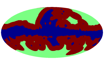
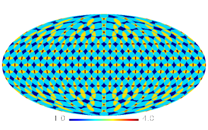
Figure 2: Illustration of the multi-resolution scheme for the missing region (left) and for the available region (right). In the left panel, the deep blue region is an example of the missing region (WMAP polarization mask), and the red area is the region used for reconstruction at working $N_{side}=64$. In the right panel are the overlapping mosaic discs at working $N_{side}=128$. When the resolution increases, the area in use decreases but the number of mosaic discs increases. In any case, each map pixel is covered at least once.

In the above schemes, for the case of estimating the missing region, the number of available pixels in use scales linearly with $N_{side}$, whereas the number of pixels to be estimated follows $N_{side}^{2}$; thus, the time cost follows $N_{side}^{3}$ for both the matrix inversion and matrix multiplication. As for the case of estimating the available region, the number of available pixels in use is nearly constant, but the number of mosaic discs follows $N_{side}^{2}$. Therefore, the overall time cost roughly follows $N_{side}^{3}$.

3.5 Lossless synthesis of multiple resolutions

By working with eq. (2.3) from $N_{side}=16$ to $N_{side}^{\prime}$, we get fullsky estimates of the CMB signal at a series of resolutions. These results should be synthesized to make a final output. The synthesis can be done either in the pixel domain or in the harmonic domain. Analysis and practical tests show that the pixel domain synthesis is not only lossless but also faster, more stable and more accurate; thus it is the default choice.

With the results at a series of resolutions starting from $N_{side}=16$, the pixel domain synthesis is done as follows:

1. First upgrade the result at $N_{side}=16$ to $N_{side}=32$, which represents larger scale structures.

2. Then downgrade the result of $N_{side}=32$ to $N_{side}=16$ and upgrade back to $N_{side}=32$.

3. Subtract the product of step 2 from the result at $N_{side}=32$ to get the difference, which represents smaller scale structures.

4. Add the product of step 3 to the product of step 1 to make the synthesized result of $N_{side}=32$.

5. Start again from step 1 with the product of step 4 to synthesize the next (higher) resolution, until reaching $N_{side}^{\prime}$.

Practically, the above procedures can also be done in a descending order from $N_{side}^{\prime}$ to $N_{side}=16$ to save the memory, and in this way, the original result at a higher resolution can be deleted after each round to free some memory.

It is easy to prove that the above synthesis procedures are lossless, i.e., when we do it with a series of multi-resolution maps downgraded from the same top-resolution map, the original map is restored by 100%. This also means the above synthesis procedures are safe for both temperature and polarizations, and will not cause a further E-to-B leakage by itself.

3.6 Matrix based fine tuning of the multi-resolution synthesis

The multi-resolution synthesis described in section 3.5 has the following matrix form: In the HEALPix pixelization scheme, each pixel at a lower resolution contains exactly four smaller pixels of the next (higher) resolution. Let the CMB signals be $S_{0}$ at this bigger pixel (lower resolution) and $S_{1-4}$ at the four smaller pixels (higher resolution), then the synthesis scheme in section 3.5 between two neighboring resolutions is described by the following matrix equation:

$$\begin{pmatrix}S_{1}\\ S_{2}\\ S_{3}\\ S_{4}\end{pmatrix}_{syn}=\frac{1}{4}\left[\begin{pmatrix}+3&-1&-1&-1\\ -1&+3&-1&-1\\ -1&-1&+3&-1\\ -1&-1&-1&+3\end{pmatrix}\cdot\begin{pmatrix}S_{1}\\ S_{2}\\ S_{3}\\ S_{4}\end{pmatrix}+\begin{pmatrix}1&1&1&1\\ 1&1&1&1\\ 1&1&1&1\\ 1&1&1&1\end{pmatrix}\cdot\begin{pmatrix}S_{0}\\ S_{0}\\ S_{0}\\ S_{0}\end{pmatrix}\right],$$ (3.4)

which can be simplified to

$$\begin{pmatrix}S_{1}\\ S_{2}\\ S_{3}\\ S_{4}\end{pmatrix}_{syn}=\frac{1}{4}\begin{pmatrix}+4&+3&-1&-1&-1\\ +4&-1&+3&-1&-1\\ +4&-1&-1&+3&-1\\ +4&-1&-1&-1&+3\end{pmatrix}\cdot\begin{pmatrix}S_{0}\\ S_{1}\\ S_{2}\\ S_{3}\\ S_{4}\end{pmatrix}=\bm{M}_{syn}\cdot\begin{pmatrix}S_{0}\\ S_{1}\\ S_{2}\\ S_{3}\\ S_{4}\end{pmatrix}$$ (3.5)

If the self-consistency condition $S_{0}=(S_{1}+S_{2}+S_{3}+S_{4})/4$ is satisfied, then $\bm{S}_{syn}=\bm{S}$, which means the synthesis scheme is lossless by itself.

However, the lossless scheme is not unique, and it is possible to design other lossless synthesis schemes by fine tuning this $4\times 5$ synthesis matrix $\bm{M}_{syn}$ to achieve a better effect. Unfortunately, this job is very time consuming; thus we leave it for the next work of this series.

3.7 Pre-processing of tiny holes in the mask

The multi-resolution scheme in section 3.4 does not work very well when the mask contains too many tiny holes, because each tiny hole will force to use some area around it for reconstruction, which is not really necessary. Therefore, if the mask contains too many tiny holes, like the ones for the point sources, then it is recommended to erase those tiny holes by the diffusive in-paint method [22, 23]. Although the diffusive in-paint method does not satisfy the minimum variance condition, it is especially safe and convenient for tiny holes in a mask, and the corresponding precision loss is usually negligible compared to the help it brings to us.

3.8 About the input CMB APS

The implementation of eq. (2.3) requires to use the CMB covariance matrix, which is determined by the input CMB APS; however, if we start from the pixel domain map directly, there is no CMB APS in advance. Therefore, we should either use a prior CMB APS, which turns the work into a typical Bayesian analysis; or we should assume an initial CMB APS, and improve it by the expectation of APS within $\{\bm{S}_{i}\}$ to get an iterative solution, which leads to a blind solution that does not depend on the prior APS. Both ways are allowed, and for the latter, the number of rounds needed to converge is roughly a few times of $1/f_{sky}$, which means when the available region is very small, the convergence can be slow. The reason for that is: when the available region is very small, it cannot provide enough correction to the fullsky APS in one round. However, in this case, the reconstruction of the missing region becomes much less important, so we can consider stopping at a lower resolution for the missing region reconstruction, and focus on the estimation of the available region, which can make the computation much faster. Another possible idea is to amplify the modification to the resulting APS by a certain factor to accelerate the convergence for a small $f_{sky}$. Both ways will be tested in the following works.

4 Test results

We start testing MrMVP in the temperature case without noise at $N_{side}=128$, with an input $\Lambda$CDM power spectrum from the most recent Planck collaboration release [27], and the mask is chosen to be the WMAP KP2 mask without the point sources. With a 4-core laptop, we generate 1,000 realizations in the constrained ensemble $\{\bm{S}_{i}\}$, and the total time cost is illustrated in figure 3 as a function of the resolution, which follows $O(N_{side}^{3})$ nicely. According to the figure, the average time cost to generate one realization at $N_{side}=128$ is about 0.1 second, which is a significantly improved speed compared to previous works.

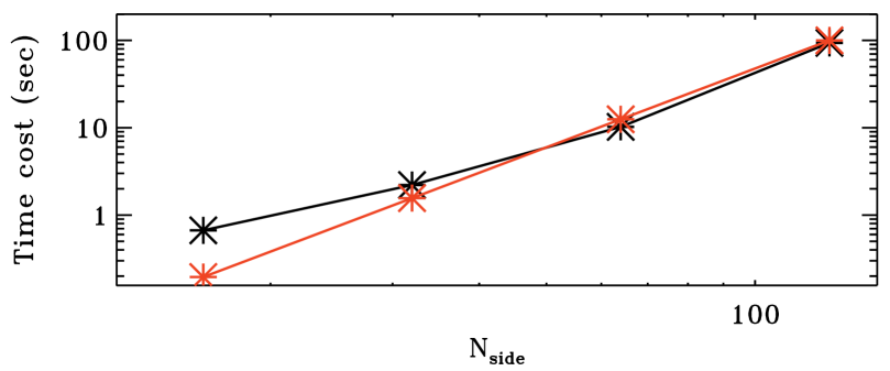
Figure 3: Illustration of the total time cost of generating 1000 realizations in $\{\bm{S}_{i}\}$ (black) from $N_{side}=16$ to $N_{side}=128$. The red line is for the $O(N_{side}^{3})$ expectation. At low resolutions, the total time cost is higher than $O(N_{side}^{3})$ due to the auxiliary operations like disk I/O, consistency test, mask and region processing, etc.

Then we compare the pixel domain expectation $\widetilde{\bm{S}}$, the input pixel domain CMB map and two constrained realizations $\bm{S}_{i}$ in figure 4. Note that $\widetilde{\bm{S}}$ is the minimum variance solution in the pixel domain, but its APS is not a minimum variance estimate of the CMB APS. The latter should be derived from the expectation of APS within $\{\bm{S}_{i}\}$.

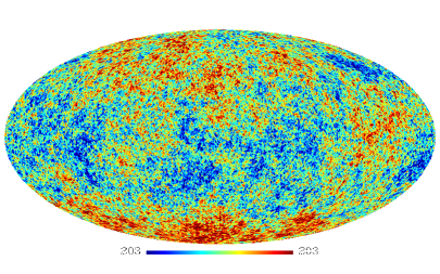
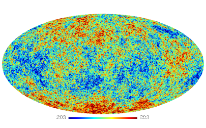
Figure 4: Comparison of the pixel domain expectation $\widetilde{\bm{S}}$ (upper-left), the input simulated CMB map (upper right), and two more constrained realizations $\bm{S}_{i}$ derived by pixel domain operations (lower panels).

In figure 5, we compare the input $\Lambda$CDM APS, the APS of the fullsky CMB map, the minimum variance estimate of the APS, and the RMS error of the minimum variance estimate. We can see that the minimum variance estimate of the APS is very well consistent with the fullsky CMB power spectrum.

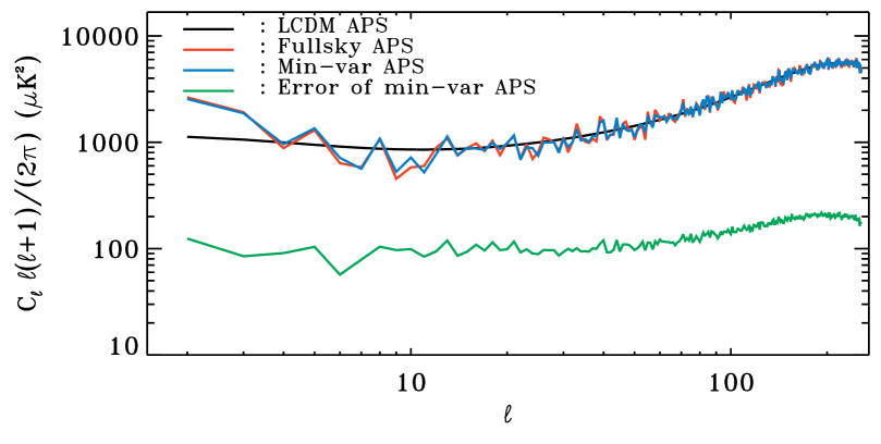
Figure 5: Comparison of the APS of the: input $\Lambda$CDM (black), fullsky CMB map (red), minimum variance estimate (blue); and the RMS error of the minimum variance estimate (green).

Note that, because the entire ensemble $\{\bm{S}_{i}\}$ are constrained, the corresponding minimum variance estimate and the error amplitudes are also constrained. Therefore, the APS error bars derived from $\{\bm{S}_{i}\}$ are more informative than a general estimation of the error bars without considering the constraint. For example, the error bar at $\ell=2$ will follow the amplitude of the true quadrupole power; thus, if the true quadrupole power happens to be quite high (like the one in figure 5), then its error bar will increase accordingly, which faithfully reflects the actual constraint from the available dataset.

For the available region, the effect of MrMVP is to alleviate the unwanted residuals. The effectiveness of alleviation is shown in figure 6, where the input signal is a simulated B-mode map with $r=0.05$, the available region is a disk in the center of the sky, and the contaminant is the residual of EB-leakage correction following the blind template correction method introduced in [28, 29, 17]. Such a residual is significantly correlated between different map pixels and is significantly non-isotropic. To make the residuals more visible and to test the method in a more difficult situation, the simulated residuals are amplified by factor 2, so they are bigger than what we may actually encounter. As we see from figure 6, the minimum variance estimate of the available region can efficiently alleviate the residual contamination, as far as its covariance matrix can be estimated.

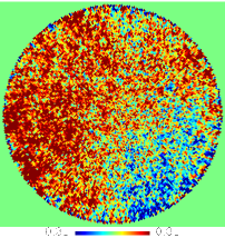
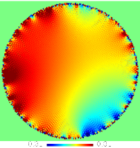
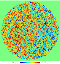
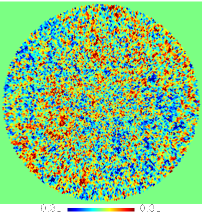
Figure 6: Illustration of the effectiveness of the minimum variance estimate of the available region. Panel 1 (from left to right) is an available region that is contaminated by the EB-leakage residuals after correction, and the residual component itself is shown in panel 2. After the minimum variance estimation, we obtain a clean region (panel 3), which is significantly improved compared to the contaminated one, and is better consistent with the true input (panel 4). The unit is $\mu$K.

In summary, figures 4–5 confirm the correctness of the MrMVP implementation, figure 3 shows that it is very fast and scaled only as $O(N_{side}^{3})$, and figure 6 shows that it can efficiently alleviate the residual errors with known covariance matrices, even if they are correlated and non-isotropic, like the residual of EB-leakage correction.

5 Conclusion and discussion

In this work, we have designed a pixel domain multi-resolution minimum variance painting method (MrMVP). Its time cost follows $O(N_{side}^{3})$, which is much better than the $O(N_{side}^{6})$ time cost of a traditional minimum variance method. The method helps to generate full sky CMB realizations that are properly constrained by the observed sky map, and a mathematical proof is given to confirm that these constrained realizations have identical statistical properties with the expected CMB signal, which is also consistent with the test results. When the method is applied to the missing region, it helps to alleviate the incomplete sky effect, and when it is applied to the available region, it can efficiently alleviate the unwanted pixel domain residuals with known covariance matrices, even if they are significantly correlated and non-isotropic, like the residual of EB-leakage. Both sides are useful in the data analysis of CMB experiments.

However, the method still need to be further developed and improved: additional routines needs to be developed to make it suitable for a complete Bayesian analysis from the pixel domain map to the final cosmological parameters; and the method itself needs to be fine tuned, especially for the synthesis matrix, to further improve its performance. Meanwhile, a GPU implementation of the method is also under consideration, because it can significantly reduce the time cost of inverting the covariance matrices. For small $f_{sky}$, several ideas of improving the convergence speed are proposed and will be tested in the following works.

References

- [1] M. Tegmark, How to measure CMB power spectra without losing information, Phys. Rev. D 55 (May, 1997) 5895–5907, [astro-ph/9611174].
- [2] D. Molinari, A. Gruppuso, G. Polenta, C. Burigana, A. De Rosa, P. Natoli et al., A comparison of CMB angular power spectrum estimators at large scales: the TT case, Mon. Not. R. Astr. Soc. 440 (May, 2014) 957–964, [1403.1089].
- [3] K. M. Górski, E. Hivon, A. J. Banday, B. D. Wandelt, F. K. Hansen, M. Reinecke et al., HEALPix: A Framework for High-Resolution Discretization and Fast Analysis of Data Distributed on the Sphere, Astrophys. J. 622 (Apr., 2005) 759–771, [astro-ph/0409513].
- [4] H. K. Eriksen, I. J. O’Dwyer, J. B. Jewell, B. D. Wandelt, D. L. Larson, K. M. Górski et al., Power Spectrum Estimation from High-Resolution Maps by Gibbs Sampling, Astrophys. J.Suppl. 155 (Dec., 2004) 227–241, [astro-ph/0407028].
- [5] J. Jewell, S. Levin and C. H. Anderson, Application of Monte Carlo Algorithms to the Bayesian Analysis of the Cosmic Microwave Background, Astrophys. J. 609 (July, 2004) 1–14, [astro-ph/0209560].
- [6] B. D. Wandelt, D. L. Larson and A. Lakshminarayanan, Global, exact cosmic microwave background data analysis using Gibbs sampling, Phys. Rev. D 70 (Oct., 2004) 083511, [astro-ph/0310080].
- [7] M. Chu, H. K. Eriksen, L. Knox, K. M. Górski, J. B. Jewell, D. L. Larson et al., Cosmological parameter constraints as derived from the Wilkinson Microwave Anisotropy Probe data via Gibbs sampling and the Blackwell-Rao estimator, Phys. Rev. D 71 (May, 2005) 103002, [astro-ph/0411737].
- [8] H. K. Eriksen, J. B. Jewell, C. Dickinson, A. J. Band ay, K. M. Górski and C. R. Lawrence, Joint Bayesian Component Separation and CMB Power Spectrum Estimation, Astrophys. J. 676 (Mar, 2008) 10–32, [0709.1058].
- [9] A. Gruppuso, A. de Rosa, P. Cabella, F. Paci, F. Finelli, P. Natoli et al., New estimates of the CMB angular power spectra from the WMAP 5 year low-resolution data, Mon. Not. R. Astr. Soc. 400 (Nov., 2009) 463–469, [0904.0789].
- [10] J. B. Jewell, H. K. Eriksen, B. D. Wandelt, I. J. O’Dwyer, G. Huey and K. M. Górski, A Markov Chain Monte Carlo Algorithm for Analysis of Low Signal-To-Noise Cosmic Microwave Background Data, Astrophys. J. 697 (May, 2009) 258–268, [0807.0624].
- [11] M. Gerbino, M. Lattanzi, M. Migliaccio, L. Pagano, L. Salvati, L. Colombo et al., Likelihood methods for CMB experiments, arXiv e-prints (Sep, 2019) arXiv:1909.09375, [1909.09375].
- [12] E. Hivon, K. M. Górski, C. B. Netterfield, B. P. Crill, S. Prunet and F. Hansen, MASTER of the Cosmic Microwave Background Anisotropy Power Spectrum: A Fast Method for Statistical Analysis of Large and Complex Cosmic Microwave Background Data Sets, Astrophys. J. 567 (Mar., 2002) 2–17, [astro-ph/0105302].
- [13] B. D. Wandelt, E. Hivon and K. M. Górski, Cosmic microwave background anisotropy power spectrum statistics for high precision cosmology, Phys. Rev. D 64 (Oct, 2001) 083003, [astro-ph/0008111].
- [14] G. Chon, A. Challinor, S. Prunet, E. Hivon and I. Szapudi, Fast estimation of polarization power spectra using correlation functions, Mon. Not. R. Astr. Soc. 350 (May, 2004) 914–926, [astro-ph/0303414].
- [15] A. Lewis, A. Challinor and N. Turok, Analysis of CMB polarization on an incomplete sky, Phys. Rev. D 65 (Jan., 2001) 023505, [astro-ph/0106536].
- [16] E. F. Bunn, M. Zaldarriaga, M. Tegmark and A. de Oliveira-Costa, E/B decomposition of finite pixelized CMB maps, Phys. Rev. D67 (2003) 023501, [astro-ph/0207338].
- [17] H. Liu, General solutions of the leakage in integral transforms and applications to the EB-leakage and detection of the cosmological gravitational wave background, Journal of Cosmology and Astroparticle Physics 2019 (oct, 2019) 001–001.
- [18] J. Kim, P. Naselsky and N. Mandolesi, Harmonic In-painting of Cosmic Microwave Background Sky by Constrained Gaussian Realization, Astrophys. J. Lett. 750 (May, 2012) L9, [1202.0188].
- [19] F. Elsner and B. D. Wandelt, Fast Wiener filtering of CMB maps, arXiv e-prints (Nov, 2012) arXiv:1211.0585, [1211.0585].
- [20] F. Elsner and B. D. Wandelt, Efficient Wiener filtering without preconditioning, Astr. Astrophys. 549 (Jan, 2013) A111, [1210.4931].
- [21] D. Kodi Ramanah, G. Lavaux and B. D. Wandelt, Wiener filter reloaded: fast signal reconstruction without preconditioning, Mon. Not. R. Astr. Soc. 468 (Jun, 2017) 1782–1793, [1702.08852].
- [22] Planck Collaboration, P. A. R. Ade, N. Aghanim, C. Armitage-Caplan, M. Arnaud, M. Ashdown et al., Planck 2013 results. XXIV. Constraints on primordial non-Gaussianity, Astr. Astrophys. 571 (Nov., 2014) A24, [1303.5084].
- [23] Planck Collaboration, P. A. R. Ade, N. Aghanim, M. Arnaud, F. Arroja, M. Ashdown et al., Planck 2015 results. XVII. Constraints on primordial non-Gaussianity, Astr. Astrophys. 594 (Sept., 2016) A17, [1502.01592].
- [24] Y. Hoffman and E. Ribak, Constrained Realizations of Gaussian Fields: A Simple Algorithm, Astrophys. J. Lett. 380 (Oct, 1991) L5.
- [25] M. Zaldarriaga, Cosmic microwave background polarization experiments, The Astrophysical Journal 503 (1998) 1.
- [26] M. Tegmark and A. de Oliveira-Costa, How to measure CMB polarization power spectra without losing information, Phys. Rev. D 64 (Sept., 2001) 063001, [astro-ph/0012120].
- [27] Planck Collaboration, N. Aghanim, Y. Akrami, M. Ashdown, J. Aumont, C. Baccigalupi et al., Planck 2018 results. VI. Cosmological parameters, arXiv e-prints (Jul, 2018) arXiv:1807.06209, [1807.06209].
- [28] H. Liu, J. Creswell, S. von Hausegger and P. Naselsky, Methods for pixel domain correction of E B leakage, Phys. Rev. D 100 (Jul, 2019) 023538, [1811.04691].
- [29] H. Liu, J. Creswell and K. Dachlythra, Blind correction of the EB-leakage in the pixel domain, Journal of Cosmology and Astroparticle Physics 2019 (apr, 2019) 046–046, [1904.00451].
- [30] The Planck data release. https://www.cosmos.esa.int/web/planck/pla, 2018.