Quantum credit loans

Abstract

Quantum models based on the mathematics of quantum mechanics (QM) have been developed in cognitive sciences, game theory and econophysics. In this work a generalization of credit loans is introduced by using the vector space formalism of QM. Operators for the debt, amortization, interest and periodic installments are defined and its mean values in an arbitrary orthonormal basis of the vectorial space give the corresponding values at each period of the loan. Endowing the vector space of dimension $M$, where $M$ is the loan duration, with a $SO(M)$ symmetry, it is possible to rotate the eigenbasis to obtain better schedule periodic payments for the borrower, by using the rotation angles of the $SO(M)$ transformation. Given that a rotation preserves the length of the vectors, the total amortization, debt and periodic installments are not changed. For a general description of the formalism introduced, the loan operator relations are given in terms of a generalized Heisenberg algebra, where finite dimensional representations are considered and commutative operators are defined for the specific loan types. The results obtained are an improvement of the usual financial instrument of credit because introduce several degrees of freedom through the rotation angles, which allows to select superposition states of the corresponding commutative operators that enables the borrower to tune the periodic installments in order to obtain better benefits without changing what the lender earns.

1 Introduction

The mathematical methods of quantum mechanics have spread outside quantum physics and have reached the field of human condition ([1], [2], [3], [4], [5] and [6]), model of decision making ([7], [8], [9], [10],[11], [12], [13], [14] and [15]), quantum game theory ([16], [17], [18], [19] and [20]), econophysics ([21], [22], [23], [24], [25], [26] and [27]) among others. This suggests us that the abstract principles of quantum mechanics exhibit a high degree of adaptability and contextuality and allow to apply it as ”quantum like” models to different branches of human cognition science. The core of quantum mechanics is the possibility of superposition and entanglement of quantum states, that physically manifest as interferences and non-local correlations of observables. Interestingly, different interpretation of quantum mechanics endow ontological reality to different mathematical objects of the theory. In particular, modal interpretations describe the quantum states as the possible properties of the system and their corresponding probabilities, and not the actual properties, where properties and facts belong to different ontological categories ([28], [29] and [30]). The relationship between the quantum state and the actual properties of the system is probabilistic, that is, the actual occurrence of a particular value of an observable is an indeterministic phenomena. Then, if quantum mechanics describes the reality, it certainly not an actual reality but a possible reality. Is the quantum superposition, only existing in potential terms, that allows to certain measurements to be actualized in a genuinely unpredictable way. This behavior can be extrapolated to other conceptual situations, for example in judgments and decisions that can be conceived as indeterministic processes when subjects give answers in situations of uncertainty, confusion or ambiguity. In turn, it can be extrapolated to model stock return distributions by considering the market force as a quantum harmonic oscillator [31] or can be used to apply quantum probability theory to formulate probabilistic models of cognition [32] and to model economical markets [33].

In this sense, the aim of this work is to contribute to the list of possible extrapolations of the abstract formalism of quantum mechanics to the field of econophysics. We will show that a particular financial instrument, the credit, can be defined over a vectorial space of dimension $M$, where $M$ is the duration of the repayment of the credit, which in the moment of contractual agreement between the lender and the borrower becomes a debt that is returned in a set of scheduled payments. It will be shown that the sequence of values for the debt, amortization, interest and periodic payments can be obtained as the eigenvalues of the respective operators in a particular eigenbasis of the vectorial space. Then, it will be shown that the basis chosen of the vector space in which the loan operators are diagonal can be rotated without changing the total amortization and the lender’s profit, computed as the sum of the periodic payments. This rotation is a manifestation of a $SO(M)$ symmetry, where $SO(M)$ is the special orthogonal group of a vectorial space of dimension $M$. Then, by endowing the vectorial space with a symmetry group, the mean values of the operators in the rotated basis allow to obtain different configurations for the debt, amortization and periodic payments, which contain the well known French and German loan systems, among others. Moreover, it will be shown that the extrapolation of the abstract mathematical structure of the quantum formalism to the credit system, can be rewritten in terms of an algebra of operators, that resembles the Heisenberg algebra of quantum mechanics. In order to be self-contained, this work will contains some elementary examples of credit loans and the generalization in a linear space, that we call “quantum credit loans”, for the purpose of introducing the machinery of the basic linear algebra which can be rather unfamiliar in the context of loans. Then, this manuscript will be organized as follows: In Section II, non-indexed credit loans are reviewed. In Section III, the recurrence relations for the debt, amortization, interest and periodic installments are described in terms of a Generalized Heisenberg algebra. Then the quantum credit loans are introduced, where the rotation transformation of the orthonormal basis is applied and the two most simple examples with $M=2$ and $M=3$ are exhaustively studied. In Section IV, indexed credit loans, where a non-constant interest rate is possible during the loan, is introduced and a particular example is studied. Finally, the conclusions are presented.

2 Non-indexed credit loans

In order to introduce the algebra of the credit loans, we can notice that these are a particular case of non-homogeneous linear recurrence relation for the debt $D$, capitalization or amortization $A$ and interest $Y$. The main difference between the loans lies in the way the amount of the installments that must be paid are computed in order to repay these loans. The French system loan is the most popular because the formula used to calculate periodical fees ensures that the periodic payment is the same for the life of the loan. This repayment includes the interest and the repayment of the capital. The only thing that will change is the proportion of what we pay of these two magnitudes: as the first increases, the second will decreases, so that the repayments are always the same. Since the debt $D$ at the beginning of the loan is very large during the initial periods, the interest $Y$ will also be greater. For this reason, we usually begin by paying a greater proportion of interest, and as time passes and the interest payments goes down, we begin to repay a greater proportion of capital $A$. Another popular system is the German system in which the periodic payment is not constant but the capital repayment is. Then, in order to express mathematically the recurrence relations of the French or German loans, we can consider an initial debt $d_{0}$, a loan duration $M$ and the interest rate $t$. The set of relations between the interest $y_{n}$, the debt $d_{n}$ and the amortization $a_{n}$ reads

$$\text{a) }q_{n}=a_{n}+y_{n}$$ (1)

$$\text{b) }y_{n}=td_{n-1}$$

$$\text{c) }d_{n+1}=d_{n}-a_{n+1}$$

the first equation 1a) means that the periodic payment or installment $q_{n}$ is composed of the interest $y_{n}$ and the amortization $a_{n}$ of the respective periodicity $n$. The second equation 1b) implies that the interest $y_{n}$ is proportional to the debt $d_{n-1}$ of the previous period and finally the last equation implies that the new debt $d_{n+1}$ is the subtraction of the debt from the last period with the current amortization. The coefficient $t$ is the interest rate. The procedure in order to compute the loan is the following: an initial debt $d_{0}$ is considered and the lapse $M$ of the loan is needed. With the initial debt, the interest $y_{1}$ is computed as $y_{1}=td_{0}$. With this value and $q_{1}$, the amortization can be computed as $a_{1}=q_{1}-y_{1}$. Finally, the new debt $d_{1}=d_{0}-a_{1}$ is obtained and the procedure starts again. As it is expected, the loan must ends, which implies that $d_{M}=0$. The boundary conditions $d_{0}=d_{0}$ and $d_{M}=0$ define a relation between the periodic installments $q_{i}$, $d_{0}$ and $M$ and determine univocally the loan series $d_{n}$, $a_{n}$, $y_{n}$ and $q_{n}$. In turn, by using eq.(1)c) and summing in $a_{n}$, we obtain that the total amortization $\sum\limits_{n=1}^{M}a_{n}=d_{0}$ must be identical to the initial debt accordingly. In the French system, $q_{n}$ is fixed and does not depend on $n$ and in the German system $a_{n}$ is fixed. Combining the three equations of eq.(1) we obtain the following recurrence relation for $d_{n}$

$$d_{n}=(1+t)d_{n-1}-q_{n}$$ (2)

which has the form of a non-homogeneous recurrence relation of the type $t_{n}=\alpha t_{n-1}+\beta_{n}$ with $\alpha=1+t$ and $\beta_{n}=-q_{n}$. The solution of the recurrence relation of eq.(2) with fixed constant $q^{(F)}$ reads

$$d_{n}^{(F)}=\frac{q^{(F)}}{t}\left[1-(1+t)^{n}\right]+(1+t)^{n}d_{0}$$ (3)

where the superscript $F$ indicates the French system loan. The boundary condition $d_{M}=0$ implies that

$$d_{M}^{(F)}=0=(1+t)^{M}\left[d_{0}+\frac{q^{(F)}}{t}\right]-\frac{q^{(F)}}{t}$$ (4)

that can be solved for $q^{(F)}$

$$q^{(F)}=\frac{d_{0}t(1+t)^{M}}{(1+t)^{M}-1}$$ (5)

or can be solved for $M$ or $d_{0}$ in the case the value of $q^{(F)}$ is fixed arbitrarily. The general procedure to obtain $q^{(F)}$ is by using $\sum\limits_{n=1}^{M}a_{n}=d_{0}$ and that $a_{n}=(1+t)a_{n-1}$ when $q_{n}=q$. Then writing $a_{1}\sum\limits_{n=1}^{M}(1+t)^{n}=d_{0}$, where $a_{1}=q-y_{1}=q-td_{0}$ is not difficult to show eq.(5). With this result, the debt $d_{n}^{(F)}$ reads

$$d_{n}^{(F)}=\frac{d_{0}}{(1+t)^{M}-1}\left[(1+t)^{M}-(1+t)^{n}\right]$$ (6)

In a similar way the amortization and the interest can be solved

$$a_{n}^{(F)}=(1+t)^{n}(q^{(F)}-td_{0})\text{ \ \ \ \ \ }y_{n+1}^{(F)}=td_{n}^{(F)}$$ (7)

In the French system, the total amount of unit currency paid is $\mathbf{Q}_{F}=q^{(F)}M=\frac{d_{0}Mt(1+t)^{M}}{(1+t)^{M}-1}$. It can be noted from eq.(2) that the debt contains a constant term $-q^{(F)}$ and, in the case that the sequence of numbers for $d_{n}$ decrease with $n$, that is, $d_{n}<d_{n-1}$, this indicates that $td_{n-1}<q^{(F)}$ and in the case that the largest value of the debt is $d_{0}$, then $t<\frac{q^{(F)}}{d_{0}}$, which implies that, in the case in which the amount to be paid $q^{(F)}$ in each period is not fixed, then the interest rate $t$ must be constrained if we expect a decreasing debt curve. This issue is not trivial, because in the case in which $t>\frac{q^{(F)}}{d_{0}}$ then $d_{n}>d_{n-1}$ and the debt increases with $n$. When the boundary condition $d_{M}=0$ is chosen, then $q^{(F)}=\frac{d_{0}t(1+t)^{M}}{(1+t)^{M}-1}$ and the inequality reads $t>0$ which is obeyed for any loan with positive interest rate $t$, that is, the boundary condition $d_{M}=0$ implies that $d_{0}>d_{M}$.

The German system consists in a constant amortization over time, that is $a_{n}=a_{0}=\frac{d_{0}}{M}$ which is obtained from $\sum\limits_{n=1}^{M}a_{n}=d_{0}$. Then the installment to be paid $q_{n}^{(G)}$ is now a function of $n$ due to eq.(1) a) as $q_{n}=y_{n}-a_{0}$. When the system of recurrence relations is solved we obtain

$$d_{n}^{(G)}=d_{0}-n\frac{d_{0}}{M}$$ (8)

$$y_{n}^{(G)}=td_{0}(1-\frac{(n-1)}{M})$$

$$q_{n}^{(G)}=\frac{d_{0}}{M}+t\frac{d_{0}}{M}(M-n+1)$$

The periodic installment is maximum for $n=1$, $q_{1}=d_{0}(t+\frac{1}{M})$, due to the fact that the interest to be paid at $n=1$ is maximum. In figure 1, the debt, the amortization, the interest and the periodic installment are shown as a function of $n$ for $t=0.02$, $d_{0}=100$ and $M=10$ for the French and German systems. As it can be seen, the debt decreases until it reaches $d_{M}=0$ in both systems and the periodic installment decreases in the German system.

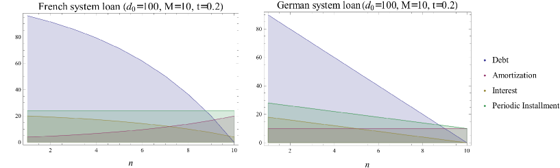
Figure 1: Non-indexed credit loan with $d_{0}=100$, $M=10$ and $t=0.2$. Left: French system. Right: German system.

The total amount paid during the loan in the German system is $\mathbf{Q}_{G}=\overset{M}{\underset{i=1}{\sum}}q_{n}^{(G)}=\frac{d_{0}}{2}\left[2+t(1+M)\right]$ that can be compared with the obtained from the French system $\mathbf{Q}_{F}=\overset{M}{\underset{i=1}{\sum}}q_{n}^{(F)}=qM$, that is larger than $\overset{M}{\underset{i=1}{\sum}}q_{n}^{(G)}$ for arbitrary values of $M$, $t$ and $d_{0}$ and allows to see why the French system is more suitable for the lender (see figure 2).

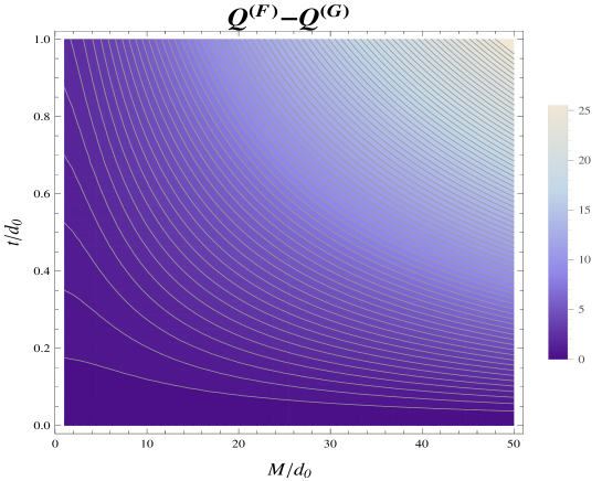
Figure 2: $\mathbf{Q}_{F}-\mathbf{Q}_{G}$ difference, where $\mathbf{Q}_{F}$ is the sum of the periodic installments in the French system and $\mathbf{Q}_{G}$ is the sum of the periodic installments in the German system for different values of $t/d_{0}$ and $M/d_{0}$.

The recurrence relations of eq.(1) allow to obtain different schedule payments $q_{n}$ by simultaneously changing the amortization schedule. In the French system, $q$ is fixed and in the German system $a_{0}$ is fixed. Both quantities are related through eq.(1a) which implies that other configurations for schedule payments should be found, for example in which $Q$ and $A$ are fixed or vary simultaneously.

3 Quantum credit loans

The mathematical structure of quantum mechanics (QM) is constructed over the concept of Hilbert spaces (see [34] and [35]). The energy of a particle is the Hamiltonian operator that acts on this Hilbert space. The eigenvalues correspond to the possible energy values of the quantum system. There is an elegant procedure to obtain the energy eigenvalues of different physical systems [36] and [37], where a generalized Heisenberg algebra (GHA) is defined and where the energy eigenvalues can be obtained from a recurrence relation derived from the algebra. In [37] the linear recurrence relation is studied identical to those obtained for the debt, amortization and interest. Then, it is interesting to derive the coupled system of recurrence relations of eq.(1) from an analogous algebra used in [37]. Due to the simultaneous magnitudes ($D$, $A$, $Y$ and $Q$) with defined values, we can further generalized the GHA by introducing several operators that commute each other as it is done in [36] to implement a three-step recurrence relation. In order to characterize the loan duration, the algebra must be defined over a finite-dimensional Hilbert space in contrast to the algebras defined in [37], where an infinite dimensional Hilbert space is constructed. The procedure to define finite dimensional Harmonic oscillator algebras was studied in [38]. In this work, we will combine both works in order to construct the finite dimensional vector space of the loan in which the GHA algebra acts. Let us define the following algebra of operators

$$\text{a) }\left[D,A\right]=\left[D,Y\right]=\left[D,Q\right]=0\text{ \ }$$ (9)

$$\text{b) }aY=f(D)a\text{\ \ \ \ c)}Ya^{{\dagger}}=a^{{\dagger}}f(D)$$

$$\text{d) }\left[D,a\right]=aA~{}\ \ \ \ \text{e) }\left[a^{{\dagger}},D\right]=Aa^{{\dagger}}$$

$$\text{f)}\ Q=Y+A\ \ \text{g) }\left[a,a^{{\dagger}}\right]=A-d_{0}\left|M\right\rangle\left\langle M\right|$$

where $D$ is the debt operator, $A$ is the amortization operator, $Y$ is the interest operator and $Q$ is the periodic installment operator. We can consider a set of $M$ orthogonal vectors $\left|n\right\rangle$ that are simultaneous eigenstates of $D$, $A$, $Y$ and $Q$. This is explicit from eq.(9 a) which implies that $D\left|n\right\rangle=d_{n}\left|n\right\rangle$, $A\left|n\right\rangle=a_{n}\left|n\right\rangle$, $Y\left|n\right\rangle=y_{n}\left|n\right\rangle$ and $Q\left|n\right\rangle=q_{n}\left|n\right\rangle$, where $d_{n}$, $a_{n}$, $y_{n}$ and $q_{n}$ are the respective eigenvalues in the eigenbasis that diagonalizes all the commuting operators. Should be noted that in the French system, the $Q$ operator is degenerate because $q_{n}=q$ and in the German system the degenerate operator is $A$. The annihilation operator $a$ and creation operator $a^{{\dagger}}$ acts on the $\left|n\right\rangle$ basis as

$$a\left|1\right\rangle = 0\text{ \ \ \ \ \ \ \ \ \ \ }a\left|n\right\rangle=N_{n}\left|n-1\right\rangle$$ (10)

$$a^{{\dagger}}\left|M\right\rangle = 0\text{ \ \ \ \ \ \ \ \ \ }a^{{\dagger}}\left|n\right\rangle=N_{n+1}\left|n+1\right\rangle$$

where $\left|M\right\rangle$ is the highest level at which the debt eigenvalue is

$$D\left|M\right\rangle=0$$ (11)

that is, the highest debt level eigenvalue is $d_{M}=0$, which implies that the loan has finished and $M$ is the loan duration and $N_{n}$ are normalization factors. Eqs.(9) b), d) and e) defines the relation between the interest, the debt and the amortization. Eq.(9) f) is the analog to eq.(1) a). Finally, eq.(9) g) defines the commutation relation between $a$ and $a^{{\dagger}}$ in terms of the amortization operator $A$. Should be noted that $Tr([a,a^{\dagger}])=0$ as it is expected. All the operators satisfy the Jacobi identity, in particular

$$\left[D,\left[a^{{\dagger}},a\right]\right]+\left[a,\left[D,a^{{\dagger}}\right]\right]+\left[a^{{\dagger}},\left[a,D\right]\right]=0$$ (12)

$$\left[D,\left[A,a\right]\right]+\left[a,\left[D,A\right]\right]+\left[A,\left[a,D\right]\right]=0$$

$$\left[D,\left[Y,a\right]\right]+\left[a,\left[D,Y\right]\right]+\left[Y,\left[a,D\right]\right]=0$$

that can be obtained by using that $\left[D,a^{{\dagger}}a\right]=0$ and that $\left[a,Y\right]=aY-Ya=(f(D)-Y)a$. The same result holds by replacing $D\rightarrow Q$ in eq.(12). In order to understand how the algebra of eq.(9) works, we can multiply by $a$ to eq.(9)f) $aQ=aY+aA$ and replacing in eq.(9)d) for $aA$ and by using eq.(9)b) we obtain

$$\left[D,a\right]=aQ-f(D)a$$ (13)

that applied to a state $\left|n\right\rangle$ gives

$$d_{n}=d_{n-1}+f(d_{n-1})-q_{n}$$ (14)

To obtain the credit loan in the French or German system we can replace the function $f(D)$ with $f(D)=(T-I)D$ where $T$ is the interest rate operator that satisfies $\left[T,D\right]=0$, $I$ is the identity operator and $T\left|n\right\rangle=(t_{n}+1)\left|n\right\rangle$. By using eq.(9) b), d) and f) we obtain

$$d_{n}=(1+t_{n-1})d_{n-1}-q_{n}~{}$$ (15)

in the case that $t_{n}=t$ and $q_{n}=q$, last equation is identical to eq.(2), where $t$ is the constant interest rate and $q$ is the fixed installment in the French system. In this case, the $T$ operator is degenerate in the $\left|n\right\rangle$ basis. Using eq.(9)g), the creation and annihilation operators can be written in the eigenbasis of the debt operator as (see eq.(6) of [38])

$$a=\overset{M-1}{\underset{j=1}{\sum}}N_{j+1}\left|j\right\rangle\left\langle j+1\right|\text{ \ \ \ \ \ \ \ \ \ }a^{{\dagger}}=\overset{M-1}{\underset{j=1}{\sum}}N_{j+1}\left|j+1\right\rangle\left\langle j\right|$$ (16)

By using last equation, the commutator $\left[a,a^{{\dagger}}\right]$ can be written as

$$\left[a,a^{{\dagger}}\right]=\overset{M-1}{\underset{j=1}{\sum}}(N_{j+1}^{2}-N_{j}^{2})\left|j\right\rangle\left\langle j\right|-N_{M}^{2}\left|M\right\rangle\left\langle M\right|$$ (17)

where we have define $N_{1}=0$. Combining last equation with the l.h.s. of eq.(9) g) we obtain

$$N_{n+1}^{2}-N_{n}^{2}=a_{n}\text{ \ \ for }n=1,2,...,M-1\text{ \ \ \ \ \ \ \ \ \ \ }N_{M}^{2}=d_{0}-a_{M}$$ (18)

and the solution reads

$$N_{j}^{2}=\overset{j-1}{\underset{i=1}{\sum}}a_{i}$$ (19)

For instance, consider the case in which $r_{i}=r=1+t$ and $q_{n}=q$ in the algebra defined in eq.(9), then the non-trivial commutation relations reduces to

$$\text{a) \ }Da^{{\dagger}}=a^{{\dagger}}((1+t)D-Q)\text{ \ \ \ b) \ }aD=((1+t)D-Q)a\text{\ \ \ \ \ }$$ (20)

$$\text{c) }\left[a,a^{{\dagger}}\right]=A-d_{0}\left|M\right\rangle\left\langle M\right|$$

which defines the desired recurrence relation for the debt in the French system. A similar analysis can be done with the German system that only differs from the French system in the choice of the non-degenerate operator, that in the German system is $A$, in contrast to the French system that choices $Q$. The function $f(D)$ is identical in both systems.

At this point is interesting to discuss the loan evolution during time. At each step $n$ of the loan, the debt, the interest, the amortization and the periodic installment actualizes. This can be represented by the mean values of these operators in the state $\left|n\right\rangle$, that is

$$\left\langle n\right|D\left|n\right\rangle = d_{n}\text{ \ \ \ \ \ \ }\left\langle n\right|Y\left|n\right\rangle=y_{n}$$ (21)

$$\left\langle n\right|A\left|n\right\rangle = a_{n}\text{ \ \ \ \ \ \ \ }\left\langle n\right|Q\left|n\right\rangle=q_{n}$$

In turn, $\left|n\right\rangle=\frac{(a^{{\dagger}})^{n}}{\prod\limits_{j=1}^{n}N_{j}}\left|1\right\rangle$, then for instance, the mean value of the debt operator reads

$$d_{n}=\frac{1}{\prod\limits_{j=1}^{n}N_{j}^{2}}\left\langle 1\right|a^{n}D(a^{{\dagger}})^{n}\left|1\right\rangle\text{ \ }$$ (22)

and by using eq.(9)e), eq.(9)f) and eq.(9) c) and that for the French system $\left[Q,a\right]=\left[Q,a^{\dagger}\right]=0$ is not difficult to show that

$$d_{n}=\left(\prod\limits_{j=1}^{n}N_{j}^{2}\right)^{-1}\left\langle 1\right|a^{n}(a^{{\dagger}})^{n}\left|1\right\rangle\left[(1+t)^{n}d_{0}-q\overset{n-1}{\underset{j=0}{\sum}}(1+t)^{j}\right]$$ (23)

but $\left(\prod\limits_{j=1}^{n}N_{j}^{2}\right)^{-1}\left\langle 1\right|a^{n}(a^{{\dagger}})^{n}\left|1\right\rangle=1$ and the result is identical to eq.(3). But then we can notice that the basis $\left|n\right\rangle$ allows to construct linear combinations, which is reasonable because the state $\left|n\right\rangle$ is an arbitrary unit vector in the vector space and it has the same status as any linear combination $\,\sum\limits_{n=1}^{M}c_{n}\left|n\right\rangle$. A linear combination of states of the loan enlarges the degrees of freedom and in turn allows the time evolution not to be constrained to the eigenvalues $d_{n}$, $y_{n}$, $a_{n}$ and $q_{n}$ of each operator at each periodicity of the loan. Besides this, the superposition of the loan states can be used to design loans that, in particular, can be a mixture of the French and the German systems. To be clear, we can consider $M=2$, then the operators $D$, $A$, $Y$, $Q$, $a$ and $a^{\dagger}$ are written in the $\{\left|1\right\rangle,\left|2\right\rangle\}$ basis as

$$D = \left(\begin{array}[]{cc}d_{1}&0\\ 0&0\end{array}\right)\text{ \ \ \ }A=\left(\begin{array}[]{cc}a_{1}&0\\ 0&a_{2}\end{array}\right)\text{ \ \ \ }Y=\left(\begin{array}[]{cc}y_{1}&0\\ 0&y_{2}\end{array}\right)$$ (30)

$$Q = \left(\begin{array}[]{cc}q_{1}&0\\ 0&q_{2}\end{array}\right)\text{ \ \ \ }a=\left(\begin{array}[]{cc}0&N_{2}\\ 0&0\end{array}\right)\text{ \ \ \ \ \ }a^{\dagger}=\left(\begin{array}[]{cc}0&0\\ N_{2}&0\end{array}\right)$$ (37)

For example in the French system we have

$$D^{(F)}=d_{0}\left(\begin{array}[]{cc}\frac{(1+t)}{(2+t)}&0\\ 0&0\end{array}\right)\text{ \ \ \ }A^{(F)}=d_{0}\left(\begin{array}[]{cc}\frac{1}{2+t}&0\\ 0&\frac{1+t}{2+t}\end{array}\right)\text{ \ \ \ }Y^{(F)}=d_{0}\left(\begin{array}[]{cc}t&0\\ 0&t\frac{1+t}{2+t}\end{array}\right)$$ (44)

$$Q^{(F)}=d_{0}\left(\begin{array}[]{cc}\frac{(1+t)^{2}}{2+t}&0\\ 0&\frac{(1+t)^{2}}{2+t}\end{array}\right)\text{ \ \ \ }a=\sqrt{d_{0}}\left(\begin{array}[]{cc}0&\sqrt{\frac{1}{2+t}}\\ 0&0\end{array}\right)\text{ \ \ \ \ \ }a^{\dagger}=\sqrt{d_{0}}\left(\begin{array}[]{cc}0&0\\ \sqrt{\frac{1}{2+t}}&0\end{array}\right)$$ (51)

and in the German system we have

$$D^{(G)}=d_{0}\left(\begin{array}[]{cc}\frac{1}{2}&0\\ 0&0\end{array}\right)\text{ \ \ \ }A^{(G)}=d_{0}\left(\begin{array}[]{cc}\frac{1}{2}&0\\ 0&\frac{1}{2}\end{array}\right)\text{ \ \ \ }Y^{(G)}=d_{0}\left(\begin{array}[]{cc}t&0\\ 0&\frac{t}{2}\end{array}\right)$$ (58)

$$Q^{(G)}=d_{0}\left(\begin{array}[]{cc}\frac{1}{2}+t&0\\ 0&\frac{1}{2}+\frac{t}{2}\end{array}\right)\text{ \ \ \ }a=\sqrt{d_{0}}\left(\begin{array}[]{cc}0&\frac{1}{\sqrt{2}}\\ 0&0\end{array}\right)\text{ \ \ \ \ \ }a^{\dagger}=\sqrt{d_{0}}\left(\begin{array}[]{cc}0&0\\ \frac{1}{\sqrt{2}}&0\end{array}\right)$$ (65)

These operators will be used in the next section in order to introduce the linear combinations. We can note that the condition $\sum\limits_{n=1}^{M}a_{n}=d_{0}$ can be written more compactly as $Tr(A)=d_{0}$. In turn, the total amount of unit currency paid $\mathbf{Q}$ by the borrower is $\mathbf{Q}=Tr(Q)$.

Then, in order to generalize the vector space formalism to $M$ dimensions, let us consider an orthogonal basis of an $M$ dimensional vectorial space where each orthogonal vector is denoted as $\left|n\right\rangle$ and let us construct $M$ orthogonal linear combinations

$$\left|\varphi_{n}\right\rangle=\sum\limits_{j=1}^{M}c_{j}^{(n)}\left|j\right\rangle\text{ \ \ \ \ \ }j=1,2,...,M$$ (66)

where $c_{j}^{(n)}$ are the coefficients of the superposition and obey

$$\sum\limits_{j=1}^{M}(c_{j}^{(m)})^{\ast}c_{j}^{(n)}=\delta_{nm}\text{ for }n\neq m$$ (67)

the eq.(66) can be written compactly as $\left|\varphi\right\rangle=U\left|\varphi_{0}\right\rangle$, where $\left|\varphi\right\rangle=\left(\left|\varphi_{1}\right\rangle\text{ }\left|\varphi_{2}\right\rangle\text{ }\cdots\text{ }\left|\varphi_{M}\right\rangle\right)^{T}$, $\left|\varphi_{0}\right\rangle=\left(\left|1\right\rangle\text{ }\left|2\right\rangle\text{ }\cdots\text{ }\left|M\right\rangle\right)^{T}$ and

$$U=\left(\begin{array}[]{cccc}c_{1}^{(1)}&c_{1}^{(2)}&...&c_{M}^{(1)}\\ c_{2}^{(1)}&c_{2}^{(2)}&\cdots&c_{2}^{(M)}\\ \vdots&\vdots&\ddots&\vdots\\ c_{M}^{(1)}&c_{M}^{(2)}&\cdots&c_{M}^{(M)}\end{array}\right)$$ (68)

The similarity transformation $U$ obeys $U^{T}U=I$ which is obtained by computing the scalar product $\left\langle\varphi\mid\varphi\right\rangle=\left\langle\varphi_{0}\right|U^{T}U\left|\varphi_{0}\right\rangle=1$. The transformation $U$ belongs to the $SO(M)$ group symmetry that preserves the distance of a vector under rotation. The $SO(M)$ is the special orthogonal group in $M$ dimensions, and the transformation $U$ is represented by a $M\times M$ matrix elements whose columns and rows are orthogonal unit vectors with $\det U=1$ [40]. The $SO(M)$ is a Lie group which can be obtained through its Lie algebra $so(M)$ by using matrix exponential of the generators of the algebra [40]. The number of the generators of the Lie algebra $so(M)$ is $g(M)=M(M-1)/2$ and is the dimension of the parameter space of $SO(M)$. These parameters are angles, then $so(M)$ is a compact group. The parameter space dimension of the $SO(M)$ is larger than the loan duration $M$ for $M>3$ which implies that the rotation transformation in the vector space of dimension $M$ provides a large number of degrees of freedom in order to tune the payment schedule with better benefits for the borrower. The transformation $U\in SO(M)$ induces a transformation on any operator $O$ as $\overline{O}=UOU^{-1}$ where $O$ can be $D$, $A$, $Y$, $Q$, $a$ and $a^{\dagger}$. For example, if $a\left|n\right\rangle=N_{n}\left|n-1\right\rangle$, then $UaU^{-1}U\left|n\right\rangle=N_{n}U\left|n-1\right\rangle$ and by calling $\overline{a}=UaU^{-1}$, $\left|\varphi_{n-1}\right\rangle=U\left|n-1\right\rangle$ and $\left|\varphi_{n}\right\rangle=U\left|n\right\rangle$, we can write $\overline{a}\left|\varphi_{n}\right\rangle=N_{n}\left|\varphi_{n-1}\right\rangle$, where $\left|\varphi_{n-1}\right\rangle$ and $\left|\varphi_{n}\right\rangle$ are two orthogonal vectors obtained from the original orthonormal basis by rotation, that is

$$\overline{a}\left|\varphi_{n}\right\rangle=N_{n}\left|\varphi_{n-1}\right\rangle\text{ \ \ \ }\overline{a}^{\dagger}\left|\varphi_{n}\right\rangle=N_{n+1}\left|\varphi_{n+1}\right\rangle$$ (69)

$$a\left|\varphi_{1}\right\rangle=0\text{ \ \ \ \ \ \ \ \ \ \ \ \ \ \ \ \ }a^{{\dagger}}\left|\varphi_{M}\right\rangle=0\text{ \ \ }$$

which means that $\overline{a}$ and $\overline{a}^{\dagger}$ acts as creation and annihilation operators of loan states in the rotated basis. The loan operators transform as

$$\overline{D} = UDU^{-1}\text{ \ \ \ \ \ }\overline{A}=UAU^{-1}$$ (70)

$$\overline{Y} = UYU^{-1}\text{ \ \ \ \ }\overline{Q}=UQU^{-1}$$

The mean values of the transformed loan operators in the original basis read

$$\left\langle n\right|\overline{D}\left|n\right\rangle = \overline{d}_{n}\text{ \ \ \ \ \ \ \ }\left\langle n\right|\overline{Y}\left|n\right\rangle=\overline{y}_{n}$$ (71)

$$\left\langle n\right|\overline{A}\left|n\right\rangle = \overline{a}_{n}\text{ \ \ \ \ \ \ }\left\langle n\right|\overline{Q}\left|n\right\rangle=\overline{q}_{n}$$

and give the expected values of the loan magnitudes at each period. Should be noted that it is meaningless to compute $\left\langle\varphi_{n}\right|\overline{O}\left|\varphi_{n}\right\rangle$ because $\left\langle\varphi_{n}\right|\overline{O}\left|\varphi_{n}\right\rangle=\left\langle n\right|O\left|n\right\rangle$ but $\left\langle n\right|\overline{O}\left|n\right\rangle=\left\langle\varphi_{n}\right|O\left|\varphi_{n}\right\rangle$. We can study the formalism for the quantum credit loans with the most simple examples $M=2$ and $M=3$.

3.1 $M=2$

As an example we can consider $M=2$, then it is possible to write the transformation from the $\{\left|1\right\rangle,\left|2\right\rangle\}$ to the $\{\left|\varphi_{1}\right\rangle,\left|\varphi_{2}\right\rangle\}$ basis as

$$\left|\varphi_{1}\right\rangle=\cos\phi\left|1\right\rangle+\sin\phi\left|2\right\rangle\text{ \ \ \ \ \ \ }\left|\varphi_{2}\right\rangle=-\sin\phi\left|1\right\rangle+\cos\phi\left|2\right\rangle$$ (72)

where $\phi\in[0,2\pi]$, $\left\langle\varphi_{1}\mid\varphi_{1}\right\rangle=\left\langle\varphi_{2}\mid\varphi_{2}\right\rangle=1$ and $\left\langle\varphi_{1}\mid\varphi_{2}\right\rangle=0$. The change of basis $\left\{\left|1\right\rangle,\left|2\right\rangle\right\}$ to $\left\{\left|\varphi_{1}\right\rangle,\left|\varphi_{2}\right\rangle\right\}$ can be obtained through a similarity transformation $U$ as

$$U=\left(\begin{array}[]{cc}\cos\phi&\sin\phi\\ -\sin\phi&\cos\phi\end{array}\right)$$ (73)

The transformation $U$ belongs to the $SO(2)$ group symmetry and can be considered as a rotation $\phi$ around the $z$ axis. In this case $g(2)=1$ and the Lie algebra $so(2)$ contains a unique generator $L=\left(\begin{array}[]{cc}0&i\\ -i&0\end{array}\right)$ such that the associated parameter is $\phi$ and $U$ of eq.(73) can be written as $U=e^{i\phi L}$. The transformed annihilation operator reads

$$\overline{a}=UaU^{-1}=N_{2}\left(\begin{array}[]{cc}-\cos\phi\sin\phi&\cos^{2}\phi\\ -\sin^{2}\phi&\cos\phi\sin\phi\end{array}\right)$$ (74)

Then, by applying $\overline{a}$ to $\overline{a}\left|\varphi_{2}\right\rangle$ we obtain that $\overline{a}\left|\varphi_{2}\right\rangle=\left|\varphi_{1}\right\rangle$, that is, $\overline{a}$ acts as an annihilation operator in the new basis. The remaining operators read

$$\overline{D}=UDU^{-1}=\left(\begin{array}[]{cc}\cos^{2}\phi d_{1}&\sin\phi\cos\phi d_{1}\\ \sin\phi\cos\phi d_{1}&\sin^{2}\phi d_{1}\end{array}\right)\text{ \ \ \ \ \ }$$ (77)

$$\overline{Y}=UYU^{-1}=\left(\begin{array}[]{cc}\cos^{2}\phi y_{1}+\sin^{2}\phi y_{2}&\sin\phi\cos\phi(y_{1}-y_{2})\\ \sin\phi\cos\phi(y_{1}-y_{2})&\sin^{2}\phi y_{1}+\cos^{2}\phi y_{2}\end{array}\right)$$ (80)

$$\overline{A}=UAU^{-1}=\left(\begin{array}[]{cc}\cos^{2}\phi a_{1}+\sin^{2}\phi a_{2}&\sin\phi\cos\phi(a_{1}-a_{2})\\ \sin\phi\cos\phi(a_{1}-a_{2})&\sin^{2}\phi a_{1}+\cos^{2}\phi a_{2}\end{array}\right)\text{ \ \ \ \ \ }$$ (83)

$$\text{\ \ \ }\overline{Q}=UQU^{-1}=\left(\begin{array}[]{cc}\cos^{2}\phi q_{1}+\sin^{2}\phi q_{2}&\sin\phi\cos\phi(q_{1}-q_{2})\\ \sin\phi\cos\phi(q_{1}-q_{2})&\sin^{2}\phi q_{1}+\cos^{2}\phi q_{2}\end{array}\right)$$ (86)

As we saw in the last section, the mean values $\left\langle n\right|\overline{D}\left|n\right\rangle$, $\left\langle n\right|\overline{A}\left|n\right\rangle$, $\left\langle n\right|\overline{Y}\left|n\right\rangle$, $\left\langle n\right|\overline{Q}\left|n\right\rangle\,$ are the actualization values for the debt, amortization, interest and periodic installment. For example, the amortizations read

$$\overline{a}_{1} = \left\langle 1\right|\overline{A}\left|1\right\rangle=\cos^{2}\phi a_{1}+\sin^{2}\phi a_{2}$$ (87)

$$\overline{a}_{2} = \left\langle 2\right|\overline{A}\left|2\right\rangle=\sin^{2}\phi a_{1}+\cos^{2}\phi a_{2}$$

and the transformed amortization obeys

$$\overline{a}_{1}+\overline{a}_{2}=a_{1}+a_{2}=d_{0}$$ (88)

as it is expected. This last equation can be obtained for any dimension $M$, because $Tr(\overline{A})=Tr(UAU^{-1})=Tr(A)=d_{0}$. In turn, the borrower that takes a loan is interested in the periodic installment schedule, that can be obtained as

$$\overline{q}_{1} = \left\langle 1\right|\overline{Q}\left|1\right\rangle=\cos^{2}\phi q_{1}+\sin^{2}\phi q_{2}$$ (89)

$$\overline{q}_{2} = \left\langle 2\right|\overline{Q}\left|2\right\rangle=\sin^{2}\phi q_{1}+\cos^{2}\phi q_{2}$$

This result is interesting because the total amount paid is $\mathbf{Q}=Tr(\overline{Q})=Tr(Q)$, so the basis rotation does not change what the lender earns. In turn, the basis rotation induces two possible superpositions of the periodic installments, then, by tuning $\phi$, it is possible to arrange two different payment schedules $\overline{q}_{1}<\overline{q}_{2}$ or $\overline{q}_{1}>\overline{q}_{2}$. The $\phi$ angle can be a parameter of the loan that the borrower can control. Interestingly, suppose the case of a borrower taking a loan of two periodic installments $M=2$. Then, suppose that before the first payment, a particular event does not allow the borrower to afford the first periodic payment. But, instead of being classified as a defaulter, the borrower can manipulate $\phi$ in order to decrease $q_{1}\rightarrow\overline{q}_{1}$ where $\overline{q}_{1}<q_{1}$. This can be achieved if the borrower chooses $\phi$ near $\pi/2$ decreasing the weight of $q_{1}$ in $\overline{q}_{1}$ (see figure 4). Once the basis is rotated, the next periodic installment is $\overline{q}_{2}$, that increases the weight of $q_{1}$ in $\overline{q}_{2}$, which means that $\overline{q}_{2}>q_{2}$. In this sense, the credit loan payments self-regulate when a rotation of the basis is applied, which is contained in the relation $Tr(Q)=Tr(\overline{Q})$, which implies for $M=2$, that $q_{1}+q_{2}=\overline{q}_{1}+\overline{q}_{2}$ and by calling $\Delta q_{1}=q_{1}-\overline{q}_{1}$ and $\Delta q_{2}=q_{2}-\overline{q}_{2}$, we have $\Delta q_{1}=-\Delta q_{2}$ and when $q_{1}>\overline{q}_{1}$ then $\overline{q}_{2}>q_{2}$. The manipulation of $\phi$ opens the possibility to the lender to offer new financial instruments for credit with the same profit but with better benefits for the borrower than the usual amortization system. Moreover, in the case of indexed interest rate with some exogenous variable, such as inflation, the basis rotation of the credit loan is suitable to control the variations of the periodic payment due to the fluctuations of the macroeconomy.

There is an inherent risk associated to the uncertainty introduced by the rotation when the borrower cannot afford the periodic payment. When this happens, a rotation basis is still available for the borrower, but then, once the basis is rotated, the payment schedule changes by decreasing the current payment and increasing the future payment. This inherent risk in the rotation procedure can be quantified by noting that the basis rotation introduces superposition of the loan states. One way to quantify this uncertainty is by computing $\Delta\overline{Q}_{n}=\sqrt{\overline{q^{2}}_{n}-\overline{q}_{n}^{2}}$ where $\overline{q}_{n}=\left\langle n\right|\overline{Q}\left|n\right\rangle$ and $\overline{q^{2}}_{n}=\left\langle n\right|\overline{Q}^{2}\left|n\right\rangle$. For example, in the case $M=2$ we obtain

$$\Delta\overline{Q}_{1} = \sqrt{(q_{1}-1)q_{1}\cos^{2}\phi+(q_{2}-1)q_{2}\sin^{2}\phi}$$ (90)

$$\Delta\overline{Q}_{2} = \sqrt{(q_{2}-1)q_{2}\cos^{2}\phi+(q_{1}-1)q_{1}\sin^{2}\phi}$$

When $\phi=\pi/2$ and $q_{2}<q_{1}$, last equation implies that $\Delta\overline{Q}_{1}=\sqrt{(q_{2}-1)q_{2}}$ and $\Delta\overline{Q}_{2}=\sqrt{(q_{1}-1)q_{1}}$, then $\Delta\overline{Q}_{2}>\Delta\overline{Q}_{1}$. That is, by selecting $\phi=\pi/2$, the borrower is paying $q_{2}$ and not $q_{1}$ at the beginning of the loan, but the future risk quantified by $\Delta\overline{Q}_{2}$ has increased. The fact that the borrower cannot paid $q_{1}$ implies that there is a potential risk that it will not be able to pay it again (it should be noted that for $\phi=\pi/2$, $\overline{q}_{1}=q_{2}$ and $\overline{q}_{2}=q_{1}$). But the borrower pays $q_{2}$ at the beginning of the loan and has time to collect $q_{1}$ meanwhile, so the risk of not paying $q_{1}$ at the second period of the loan must be less than the initial risk of not paying $q_{1}$ at the beginning of the loan. For each rotation basis chosen at each period of the loan there is a risk flow that should be used as a complement to the quantum credit loans in order to ensure a measure of the risk to be used by the lender when the borrower applies a rotation of the loan states. In Table 1 it can be seen the main difference between the usual credit loan and the quantum credit loan for $M=2$.

$$M=2$$ Debt Interest Amortization Installment

Usual

Credit Loan

Quantum

Credit Loan

$$\text{Table 1. Usual credit loan compared with quantum credit loan for }M=2\text{.}$$

Should be stressed that the condition $Tr(\overline{A})=Tr(A)=d_{0}$ implies that $q_{2}=(1+t)\left[(1+t)d_{0}-q_{1}\right]$, then there is only one arbitrary parameter $q_{1}$ in a general credit loan with $M=2$ and the transformed periodic installments can be written as

$$\overline{q}_{1} = (\cos^{2}\phi-(1+t)\sin^{2}\phi)q_{1}+(1+t)^{2}\sin^{2}\phi d_{0}$$ (91)

$$\overline{q}_{2} = (\sin^{2}\phi-(1+t)\cos^{2}\phi)q_{1}+(1+t)^{2}\cos^{2}\phi d_{0}$$

where now the transformed periodic installments are written in terms of the initial debt taken by the borrower and the first payment. This representation of the transformed $\overline{q}_{i}$ is suitable to fix $q_{1}=0$, that is, the initial payment of the non-rotated credit loan vanishes and then $\overline{q}_{1}=\sin^{2}\phi(1+t)^{2}d_{0}$ and $\overline{q}_{2}=\cos^{2}\phi(1+t)^{2}d_{0}$ which makes explicit the modulation in $\phi$ introduced by the rotation in the $\overline{q}_{i}$.

Now, let us consider the known loan systems: the French and German system. In the French system, $q_{1}^{(F)}=q_{2}^{(F)}=q^{(F)}=d_{0}\frac{(1+t)^{2}}{2+t}$ and then $\overline{q}_{1}^{(F)}=\overline{q}_{2}^{(F)}=q^{(F)}$. This is expected because in the French system, the periodic installment operator is diagonal $Q^{(F)}I$, then $UQ^{(F)}IU^{-1}=Q^{(F)}$. In the German system, $q_{1}^{(G)}=\frac{d_{0}}{2}+td_{0}$ and $q_{2}^{(G)}=\frac{d_{0}}{2}+t\frac{d_{0}}{2}$, then

$$\overline{q}_{1}^{(G)} = \left\langle 1\right|\overline{Q}\left|1\right\rangle=\frac{d_{0}}{2}+td_{0}\left(1-\frac{1}{2}\sin^{2}\phi\right)$$ (92)

$$\overline{q}_{2}^{(G)} = \left\langle 2\right|\overline{Q}\left|2\right\rangle=\frac{d_{0}}{2}+td_{0}\left(\frac{1}{2}+\frac{1}{2}\sin^{2}\phi\right)$$

Should be noted that, as it happens in the transformed amortization, the sum of the periodic installments does not depend on $\phi$, that is, $\overline{q}_{1}+\overline{q}_{2}=q_{1}+q_{2}$. We can transform the German system with $q_{1}^{(G)}\neq q_{2}^{(G)}$ into a loan system with identical periodic installments $\overline{q}_{1}^{(G)}=\overline{q}_{2}^{(G)}$. By using last equation this condition is obeyed when $\sin\phi=\frac{1}{\sqrt{2}}$ which is satisfied for $\phi=\pi/4$. Replacing this value in $\overline{q}_{1}^{(G)}$ or $\overline{q}_{2}^{(G)}$ we obtain $\overline{q}^{(G)}=\frac{d_{0}}{2}(1+\frac{3}{2}t)$. Then by rotating the basis we can transform a non-constant periodic payment schedule into a constant periodic payment schedule. Must be stressed that the amortizations in the German system are constant and remain the same after the $\phi=\pi/4$ rotation. Then, the new loan system is not exactly a French system but a mixture of both, that is, the transformed loan have constant periodic installments and constant amortizations but the periodic installment obtained $\overline{q}^{(G)}=\frac{D_{0}}{2}(1+\frac{3}{2}t)$ is not identical to the periodic installments of the French system $q^{(F)}=d_{0}\frac{(1+t)^{2}}{2+t}$. This new mixed French-German system credit loan cannot be obtained by the usual formalism of eq.(1) because if $q_{n}$ and $a_{n}$ are constants then $y_{n}$ and $d_{n}$ cannot change. The relation between quantum credit loans and normal credit loans is analogue to the relation between quantum game theory and classical game theory, where in the quantum theory, the set of possible strategies is enlarged by interfering strategies ([41] and [42]). The same procedure is introduced with the quantum credit loans by enlarging the set of repayment schedules by, for example, interfering normal repayment schedules. In turn, a path integral formulation of credit loans could be constructed with an appropriate Lagrangian, where the probability amplitude for a particular path in the debt space (two possible different paths can be with constant amortization and the other with constant periodic installment) can be calculated with an action $S=\int L(t)dt$. Interfering paths can be constructed with $e^{iS}$ as it is used in the Feynman path integral formulation in quantum mechanics or other quantum model of the stock market ([43] and [44]). Finally, an interesting fact about rewriting the credit loan in a vector space is that we have the freedom to choose any linear combination of the states of the loan. There are particular quantum states in physics that are called coherent states whose dynamics closely resembles the oscillatory behavior of a classical harmonic oscillator, and is widely familiar in quantum optics because it describes the maximal coherence and classical behavior of the quantum electromagnetic field. This is realized as laser light that emit photons in a highly coherent frequency mode inside a cavity [45]. In [38], the coherent states of $M=2$ is obtained in Appendix (eq.A6), where a non-trivial phase appears. In the particular case of $M=2$, the mean values of the loan operators in the coherent state are identical to those obtained in eq.(77) but it is expected that for $M>2$, interesting differences between the rotated and coherent states can be used to improve the loan properties.

3.2 $M=3$

We can go further in the analysis of the basis rotation by considering a credit loan of duration $M=3$. The orthogonal group $SO(3)$ can be constructed through its Lie algebra $so(3)$ that contains three generators $L_{1}$, $L_{2}$ and $L_{3}$ that corresponds to antisymmetric $3\times 3$ matrices in the adjoint representation [40]. The transformation $U$ can be computed as $U=e^{i\theta L_{1}}e^{i\gamma L_{2}}e^{i\phi L_{3}}$. Then, by writing $B=\{\left|1\right\rangle,\left|2\right\rangle,\left|3\right\rangle\}$, the basis rotation reads

$$\left|\varphi_{1}\right\rangle=\sin\theta\cos\phi\left|1\right\rangle+\cos\theta\cos\phi\left|2\right\rangle-\sin\phi\left|3\right\rangle$$ (93)

$$\left|\varphi_{2}\right\rangle=(\sin\theta\sin\phi\sin\gamma+\cos\theta\cos\gamma)\left|1\right\rangle+(\cos\theta\sin\phi\sin\gamma-\sin\theta\cos\gamma)\left|2\right\rangle+\cos\phi\sin\gamma\left|3\right\rangle$$

$$\left|\varphi_{3}\right\rangle=(\cos\theta\sin\gamma+\sin\theta\sin\phi\cos\gamma)\left|1\right\rangle+(\cos\theta\sin\phi-\sin\theta\sin\gamma)\left|2\right\rangle+\cos\phi\cos\gamma\left|3\right\rangle$$

and the similarity transformation $U^{(3)}$ reads

$$U^{(3)}=\left(\begin{array}[]{ccc}\sin\theta\cos\phi&\sin\theta\sin\phi\sin\gamma+\cos\theta\cos\phi\cos\gamma&\sin\theta\sin\phi\cos\gamma+\cos\theta\sin\gamma\\ \cos\theta\cos\phi&\cos\theta\sin\phi\sin\gamma-\sin\theta\cos\gamma&\cos\theta\sin\phi\cos\gamma-\sin\theta\sin\gamma\\ -\sin\phi&\cos\phi\sin\gamma&\cos\phi\cos\gamma\end{array}\right)$$ (94)

where we have three arbitrary angles $\theta,\phi$ and $\gamma$ to manipulate freely which defines the parameter space of $SO(3)$. The transformation of the periodic installment operator $\overline{Q}=UQU^{-1}$ allows us to obtain the mean values $\left\langle n\right|\overline{Q}\left|n\right\rangle$ as

$$\overline{q}_{1}=\left\langle 1\right|\overline{Q}\left|1\right\rangle=\sin^{2}\theta\cos^{2}\phi q_{1}+\sec(2\gamma)\cos^{2}\theta(\cos^{2}\gamma q_{2}-\sin^{2}\gamma q_{3})+$$ (95)

$$\sec(2\gamma)\sin^{2}\theta\sin^{2}\phi(\cos^{2}\gamma q_{3}-\sin^{2}\gamma q_{2})$$

$$\overline{q}_{2}=\left\langle 2\right|\overline{Q}\left|2\right\rangle=\cos^{2}\theta\cos^{2}\phi q_{1}+\sec(2\gamma)\sin^{2}\theta(\cos^{2}\gamma q_{2}-\sin^{2}\gamma q_{3})+$$

$$\sec(2\gamma)\cos^{2}\theta\sin^{2}\phi(\cos^{2}\gamma q_{3}-\sin^{2}\gamma q_{2})$$

$$\overline{q}_{3}=\left\langle 3\right|\overline{Q}\left|3\right\rangle=\sin^{2}\phi q_{1}+\sec(2\gamma)\cos^{2}\phi(\cos^{2}\gamma q_{3}-\sin^{2}\gamma q_{2})$$

Should be noted that when $\gamma=\frac{\pi}{2}$ and $\theta=0$ we recover a rotation $\phi$ around the $\left|3\right\rangle$ axis. Now there are three parameters to be tuned in order to satisfy the best periodic payment schedule for the borrower. By writing $\sin\phi=x$, $\sin\theta=y$ and $\sin\gamma=z$ last equation can be rewritten as

$$\overline{q}_{1}=y^{2}(1-x^{2})q_{1}+\frac{1-y^{2}}{1-2z^{2}}\left[(1-z^{2})q_{2}-z^{2}q_{3}\right]+\frac{x^{2}y^{2}}{1-2z^{2}}\left[(1-z^{2})q_{3}-z^{2}q_{2}\right]$$ (96)

$$\overline{q}_{2}=(1-x^{2})(1-y^{2})q_{1}+\frac{y^{2}}{1-2z^{2}}\left[(1-z^{2})q_{2}-z^{2}q_{3}\right]+\frac{x^{2}(1-y^{2})}{1-2z^{2}}\left[(1-z^{2})q_{3}-z^{2}q_{2}\right]$$

$$\overline{q}_{3}=x^{2}q_{1}+\frac{1-x^{2}}{1-2z^{2}}\left[(1-z^{2})q_{3}-z^{2}q_{2}\right]$$

These set of equations for the periodic payments $\overline{q}_{i}$ as a function of $x$, $y$ and $z$ provide a large set of degrees of freedom in order to manipulate the payment schedule.

4 Quantum indexed credit loans

In order to introduce the indexed credit loans in terms of the GHA, we can recall eq.(14)

$$d_{n}=(1+t_{n-1})d_{n-1}-q_{n}$$

where in this case the interest rate $t_{n}$ depends on $n$. A particular example of this loan, is the UVA credit loan in Argentina, where the UVA (Unidad de Valor Adquisitivo [46]) is a new variable and the loan contract is made in units of UVA and not in Argentinian monetary unit (Argentinian Pesos). The UVA is related to the Argentinian unit currency as $u_{n}=\alpha\times 1$peso, where $\alpha$ is a number that varies from day to day and is computed by using the Consumer’s price index (CPI). The procedure to create this relation between UVA and CPI is by indexing $\alpha$ to the Reference Stability Coefficient Rate (CER) coefficient [47] which is elaborated by the Central Bank and depends on the Argentinian inflation. That is, the units of UVA depend on the Inflation or Consumer’s Index Price. The UVA credit loan is a French system loan in the UVA units but the borrower makes the payment in Argentinian monetary unit. Then the amount to be paid periodically is $q_{n}=u_{n}q$ where $q$ is the periodic payment in UVA units obtained from the French system and $u_{n}$ is the price of the UVA unit in term of the Argentinian monetary unit. Then, although the periodic payment is in UVA units and is constant in time, the amount to be paid with Argentinian monetary unit varies with time because the UVA price in terms of Argentinian pesos depends on time. Going further, although the debt in UVA unit follows the same behavior as the debt in the non-indexed French system, the debt in Argentinian monetary unit for the indexed loan follows a different behavior. That is, although the debt $d_{n}$ in UVA unit decreases, the debt in Argentinian monetary unit is variable. Computing the amount of debt in Pesos as

$$\overline{d}_{n}=d_{n}u_{n}$$ (97)

Then it can be shown that $\overline{d}_{n}$ follows the recurrence relation

$$\overline{d}_{n}=(1+t)\frac{u_{n}}{u_{n-1}}\overline{d}_{n-1}-u_{n}q$$ (98)

which implies an effective indexed interest rate $t_{n-1}=(1+t)\frac{u_{n}}{u_{n-1}}-1$. If $\frac{u_{n}}{u_{n-1}}=1$, $t_{n-1}=t$ as it is expected. From eq.(99), when $u_{n}$ increases with $n$ and $d_{n}$ decreases, there is a maximum value that can be obtained through the equation $\frac{d}{dn}(\overline{d}_{n})=\frac{d}{dn}(d_{n})u_{n}+d_{n}\frac{du_{n}}{dn}=0$ for a particular value $n$. In figure 3 the behavior of the debt, interest, amortization and periodic payment is shown as a function of $n$ when the UVA credit loan follows the French system (left) and when follows the German system (right). In the figure 3 it can be seen that the debt $\overline{d}_{n}$ in the German system does not present a peak because the schedule payment $q_{n}^{(G)}$ decreases with $n$ and balance the increment due to $u_{n}$.

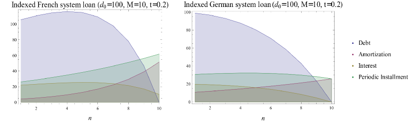
Figure 3: Indexed credit loan with $d_{0}=100$, $M=10$, $t=0.2\,$ and $u_{n}=a^{n}$ where $a=1.1$. Left: French system. Right: German system.

To introduce the indexed UVA credit loans in terms of GHA, we can recall the function $f(D)$ of eq.(9) that is replaced by $f(D)=(T-I)D$ where $T$ is the interest rate operator that satisfies $\left[T,D\right]=0$, $I$ is the identity operator and $T\left|n\right\rangle=t_{n}\left|n\right\rangle$ where $t_{n}=(1+t)\frac{u_{n+1}}{u_{n}}-1$ in the particular case of the UVA credit loan. For simplicity we can consider $M=2$ and the transformed periodic payments read

$$\overline{q}_{1} = \cos^{2}\phi u_{1}q+\sin^{2}\phi u_{2}q$$ (99)

$$\overline{q}_{2} = \sin^{2}\phi u_{1}q+\cos^{2}\phi u_{2}q$$

For simplicity we can write $u_{2}=au_{1}$ where $a$ is the inflation rate between the two periods of the loan and we obtain

$$\frac{\overline{q}_{1}}{u_{1}q} = \cos^{2}\phi+a\sin^{2}\phi$$ (100)

$$\frac{\overline{q}_{2}}{u_{1}q} = \sin^{2}\phi+a\cos^{2}\phi$$

then we can find that $\overline{q}_{1}=\overline{q}_{2}$ for $\phi=\pi/4$ and we have transformed the indexed credit loan into a constant periodic installment loan (see figure 4), where this constant is $\overline{q}_{1}(\phi=\frac{\pi}{4})=\overline{q}_{2}(\phi=\frac{\pi}{4})=\frac{1}{2}(1+a)u_{1}q$.

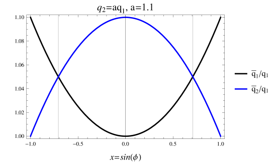
Figure 4: Transformed periodic installments $\overline{q}_{1}/q_{1}$ and $\overline{q}_{2}/q_{1}$ as a function of $x=\sin\phi$ with $a=1.1$. Vertical lines indicates the values $x=\pm 1/\sqrt{2}$.

Then we obtain

$$\overline{q}_{1}(\phi=\frac{\pi}{4})=(\frac{1}{2}+\frac{a}{2})q_{1}\text{ \ \ \ \ \ \ \ \ \ }\overline{q}_{2}(\phi=\frac{\pi}{4})=(\frac{1}{2}+\frac{1}{2a})q_{2}$$ (101)

which in the case $a>1$, $\overline{q}_{1}>q_{1}$ but $\overline{q}_{2}<q_{2}$ as it was shown in the last section. That is, we compensate the extra amount paid in the first period by paying $\overline{q}_{2}<q_{2}$. For $M=2$ the angle of the rotation $\phi$ does not depend on $a$. By considering $M=3$ and considering a constant inflation rate $a$, then $u_{2}=au_{1}$ and $u_{3}=au_{2}=a^{2}u_{1}$, then we can compute the conditions for $x$, $y$ and $z$ in order to have the possible configuration $\overline{q}_{1}-q_{1}<0$, $\overline{q}_{2}-q_{2}<0$ and $\overline{q}_{3}-q_{3}>0$ (figure 5). The shaded region with the specific values $z=0.6$ and $z=0.7$ indicates possible values for $x$ and $y$ that allows the configuration to be achieved. The different schedules can be given by noting that $\overline{q}_{1}-q_{1}+\overline{q}_{2}-q_{2}+\overline{q}_{3}-q_{3}=0$, then in the case $\overline{q}_{1}-q_{1}<0$, then $q_{2}-\overline{q}_{2}<\overline{q}_{3}-q_{3}$, which implies that the transformed schedule payment contains at least one transformed periodic payment that is larger than the non-transformed one.

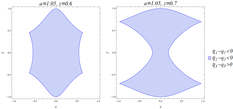
Figure 5: Regions where $\overline{q}_{1}-q_{1}<0$, $\overline{q}_{2}-q_{2}<0$ and $\overline{q}_{3}-q_{3}>0$ holds, with $a=1.05$. Right: $z=\sin\gamma=0.6$. Left: $z=\sin\gamma=0.7$.  

An interesting point to be discussed is that the dependence of $u_{n}$ with $n$ cannot be known because the inflation rate is actualized periodically and this value depends on several factors, such as the monetary basis, dollar price, etc. The similarity transformation $U$ implies that the transformed periodic payments are a superposition of the original periodic payments, but these cannot be known at the beginning of the loan because of the lack of knowledge of $u_{n}$. If for simplicity we consider again $M=3$ and suppose that the first payment cannot be addressed by the borrower, a rotation is still available that gives eq.(99) where $u_{1}$ is known but $u_{2}$ and $u_{3}$ are not known. The customer needs to perform a rotation in such a way to obtain $\overline{q}_{1}<q_{1}=u_{1}q$. At this point it could be necessary to consider the future inflation expectations in order, at least, to define a probability density function $p(u_{2},u_{3})$ that obeys $\int_{0}^{u_{\max}}\int_{0}^{u_{\max}}du_{2}du_{3}p(u_{2},u_{3})=1$, in such a way to determine the best option for the customer. By using eq.(96), it can be seen that $\overline{q}_{i}=\overline{q}_{i}(q_{1},x,y,z,u_{1},u_{2},u_{3})$, then we can compute $\left\langle\overline{Q}_{i}\right\rangle=\int_{0}^{u_{\max}}\int_{0}^{u_{\max}}du_{2}du_{3}p(u_{2},u_{3})\overline{Q}_{i}(q_{1},x,y,z,u_{1},u_{2},u_{3})$, where $u_{\max}$ is an upper bound for the indexed variable and then consider the most suitable election of $x$, $y$ and $z$ as a function of $u_{\max}$ for the borrower. Another solution is to model the future expectation inflation by some particular function $u_{n}$. In the Argentinian case, by fitting the real values of $u_{n}$ [46] there are two possible reliable solutions: a power law fitting $u_{n}=u_{0}e^{\alpha n}$ where $\alpha\sim 0.0109$ and $u_{0}=14.27$ and a linear fitting $u_{n}=u_{0}+0.03n$. Any of these two fittings allow to rotate the basis of the Hilbert space of the loan in a specific way to obtain, for example, constant periodic payments, giving predictability to the borrower.

The general procedure for large $M$, such as mortgage loans, that can be have a duration of $20$ or $30$ years, implies to develop complex strategies in order to take advantage of the large matrix transformation $U$ and the different payment schedules that can be obtained from the equation $Tr(\overline{Q})=Tr(Q)$. These strategies involve to use the mathematical machinery of group theory in order to use the subgroups of $SO(M)$ to introduce selective payment schedules and can contribute to the analysis of quantum finance interest rate models ([48], [49]). For example, in the case $M=3$ we can consider a rotation subgroup as

$$U=\left(\begin{array}[]{ccc}\cos\phi&\sin\phi&0\\ -\sin\phi&\cos\phi&0\\ 0&0&1\end{array}\right)$$ (102)

which implies not altering the $q_{3}$ payment. This is a particular case of $SO(2)\subset SO(3)$. A large classification of subgroups of $SO(M)$ can be found in the literature in terms of cosets, conjugacy classes, etc (see [40] chapter 19 to 25). From the perspective of the Lie algebra $so(M)$, the subgroups can be found by exponential map of the specific generators of the rotation. In turn, using the Lie algebra it is possible to obtain, for example in the case $M=4$ that $so(4)=so(3)\oplus so(3)$. By computing the exponential map of the generators of each $so(3)$ it is possible to obtain specific subgroup of rotations according to the customer needs. This procedure can be generalized for large $M$ without complications, although implementing a software that allows to manipulate the entire parameter space of the Lie algebra and to select specific subgroups of $SO(M)$ through the Lie algebras should be extremely necessary. To make a final remark, the generalized Heisenberg algebra is suitable to be applied to quantum finance related to index-linked coupons that depends on market defined index [50]. In turn, diverse Hamiltonians are defined to model the stock market. For example, in [51] in which a quantum anharmonic oscillator is used as a model for the stock market. The motion of the stock price is modeled as the dynamics of a quantum particle and the probability distribution of price return is computed with the wave function obtained from the Scrhodinger equation with an anharmonic oscillator potential. The Black-Scholes equation can be mapped into the Schrodinger equation (see [52] and [53]) and a Hamiltonian operator with potential can be constructed. Interesting approaches using non-Hermitian Hamiltonians are given in [54]. In [55] a finite dimensional Hilbert space is constructed to model the stock market that isomorphic to $\mathbb{C}^{d}$, where $d$ is the discrete number of possible rates of return. In [39] all possible realizations of investors holding securities and cash is taken as the basis of the Hilbert space of market states. The temporal evolution of an isolated market is unitary in this space. In [56], the quantum framework is used to model supply and demand. The different potentials appearing in the Hamiltonians of the different models of the stock market can be studied using the generalized Heisenberg algebras (see [57]). Then, having access to the algebra of observables of a quantum system allows us to design better general quantum models for stock price or financial instruments instead of using a particular representation of the wavefunction (the coordinate representation) that is not more than a particular representation of the underlying algebra.

Finally, should be stressed that the commutative operators chosen to define the loan systems (eq.(9)a) is suitable to generalize via non-commutative operators, which can be used to capture the impossibility of a joint measurement of these quantities and hence can explain the existence of order effects and deeper levels of ambiguity in respect to the loan realization. In turn, the quantum formalism introduced for credits is suitable to consider repackaging of different types of loans such as credit loans, credit card debt, business loans and mortgage into pools, because these pools can be modeled as tensor product of the algebras. The symmetry group of the tensor product of the algebras will allows to construct entangled loan states, without changing the return because $Tr(\overline{Q}_{1}\otimes\overline{Q}_{2}\otimes...\otimes\overline{Q}_{n})=Tr(Q_{1}\otimes Q_{2}\otimes...\otimes Q_{n})$.

5 Conclusions

In this work we have shown a generalization of a credit loan by introducing linear operators for the debt, amortization, interest and periodic installments that act on a vector space of dimension $M$, where $M$ is the loan duration. We have shown that endowing this vector space with an $SO(M)$ symmetry, a basis rotation of the orthonormal basis allows us to change the schedule of the periodic payments, allowing better benefits for the borrower in the case a payment cannot be afford or any other circumstance in which a default of the remaining debt is possible. The values of the loan operators are computed as mean values of these operators in any of the orthogonal vectors of the eigenbasis of the vector space. In turn, the rotation basis does not change the total amortization and the total amount paid by the borrower, which is expected in order not to change what the lender earns and simultaneously not to change what the borrower amortizes. In turn, it was shown that a generalized Heisenberg algebra for the loan operators can be defined that gives the usual recurrence relations for the debt, amortization, interest and periodic installments. Finally, the case of indexed credit loans is studied, where the rotation basis provides a sophisticated solution when the periodic installments depend on exogenous variables with a non-predictive behavior. Some particular cases with $M=2$ and $M=3$ are studied showing how the rotation transformation can be applied to design specific schedule periodic payments.

6 Acknowledgments

This paper was partially supported by grants of CONICET (Argentina National Research Council) and Universidad Nacional del Sur (UNS) and by ANPCyT through PICT 1770, and PIP-CONICET Nos. 114-200901-00272 and 114-200901-00068 research grants, as well as by SGCyT-UNS., J. S. A. is a member of CONICET.

References

- [1] D. Aerts, The entity and modern physics: the creation discovery view of reality. In E. Castellani (Ed.), Interpreting bodies: Classical and quantum objects in modern physics (pp. 223–257). Princeton: Princeton Unversity Press (1998).
- [2] R. F. Bordley, Oper. Res. 46, 923–926 (1998).
- [3] D. Aerts, and S. Aerts, Found. Sci. 1, 85–97 (1994).
- [4] D. Aerts, J. Broekaert, L. Gabora, and S. Sozzo, Behavioral and Brain Sciences, 36, 274–276 (2013).
- [5] A.Y. Khrennikov, Found. Phys. 29, 1065–1098 (1999).
- [6] H. Atmanspacher, H. Römer and H. Walach, Found.Phys. 32, 379–406 (2002).
- [7] J. R. Busemeyer, and P. D. Bruza, Quantum Models of Cognition and Decision (Cambridge University Press), (2014).
- [8] D. Aerts, Journ. Math. Psychology, 53(5), 314-348 (2009).
- [9] A. L. Mogiliansky, S. Zamir and H. Zwirn, Journ. Math. Psychology, 53(5), 349-361 (2009).
- [10] V. Yukalov and D. Sornette, Theory and Decision, 70(3), 283-328 (2011)..
- [11] A. Khrennikov, Ubiquitous Quantum Structure: From Psychology to Finance (Springer, Berlin), (2010).
- [12] E. M. Pothos and J. R. Busemeyer, Proc. R. Soc. B, 276, 2171 (2009)..
- [13] Z. Wang, J. R. Busemeyer, H. Atmanspacher, E. M. Pothos, Top. Cogn. Sci. 5(4):672-688 (2013) .
- [14] W. M. Gervais and A. Norenzayan, Science 336, 493 (2012).
- [15] T. Boyer-Kassema, S. Duchênec, E. Guerci, Mathematical Social Sciences 80, 33–46 (2016).
- [16] D. A. Meyer, Phys. Rev. Lett. 82, 1052–1055 (1999).
- [17] E. Klarreich, Nature 414, 244–245 (2001).
- [18] J. Eisert, M. Wilkens and M. Lewenstein, Phys. Rev. Lett., 83, 3077–3080 (1999) .
- [19] J. Du, X. Xu, H. Li, X. Zhou and R. Han, Phys. Lett. A, 289 9–15 (2001).
- [20] L. Marinatto and T. Weber, Phys. Lett. A, 27, 291–303 (2000).
- [21] M. Schaden, A Quantum Approach to Stock Price Fluctuations,arXiv:physics/0205053.
- [22] F. Bagarello, A quantum statistical approach to simplified stock mar- kets, Physica A: Statistical Mechanics and its Applications, 388(20):4397-4406 (2009).
- [23] O. A. Choustova, Quantum Bohmian model for financial market, Physica A: Statistical Mechanics and its Applications, 374(1):304–314 (2007).
- [24] A. Atalluah, I. Davidson, M. Tippett, Physica A: Statistical Mechanics and its Applications, 388(4):455-461 (2009).
- [25] B. E Baaquie, Path Integrals and Hamiltonians: Principles and Methods. Cambridge University Press, (2014).
- [26] E. W. Piotrowski and J. Sładkowski, Physica A, 387, 3949-3953 (2008).
- [27] E. W. Piotrowski and J. Sładkowski, Quantitative Finance, 4:6, 61-67 (2004).
- [28] Ardenghi, J. S., Castagnino, M. y Lombardi, O., Found. Phys., 39, 1023,(2009).
- [29] Lombardi, O., Castagnino, M. y Ardenghi, J. S., Stud. Hist. Phil. Mod. Phys., 41, 93, (2010).
- [30] Ardenghi, J. S., Castagnino, M. y Lombardi O., Int. J. Theor. Phys., 50, 774, (2011).
- [31] K. Ahn, M. Y. Choi, B. Dai, S. Sohn and B. Yang, Europhysics Letters, 120, 3 (2018)
- [32] P. D. Bruza, Z. Wang and J. R. Busemeyer, Trends in Cognitive Sciences, 19, 7 (2015).
- [33] L. Smolin, arXiv:0902.4274v1 (2009).
- [34] Ballentine, L. (1998). Quantum Mechanics: A Modern Development. Singapore: World Scientific.
- [35] A. Messiah, Quantum Mechanics, vol I, North-Holland (1961).
- [36] J. de Souza, E. M. F. Curado, M. A. Rego-Monteiro, Journ. Physics A: Math. Gen., 39 10415 (2006).
- [37] E. M. F. Curado and M. A. Rego-Monteiro, J. Phys. A, 34, 3253(2001).
- [38] V. Buzek, A. D. Wilson-Gordon, P. L. Knight and W. K. Lai, Phys. Rev. A, 45, 11 (1992).
- [39] M. Schaden, Physica A, 316, 1-4, 511-538 (2002).
- [40] H. Georgi, Lie Algebras in Particle Physics, 2nd edition, Frontiers in Physics (WestView Press) (1999).
- [41] E.W. Piotrowski, J. Sładkowski, Physica A 312, 208 (2002).
- [42] A. P. Flitney, D. Abbott, Physica A 324 152 (2003).
- [43] G. Montagna, O. Nicrosini and N. Moreni, Physica A, 310, 450-466 (2002).
- [44] E. Jimenez and D. Moya, Physica A 348, 505-543 (2005).
- [45] C. Cohen-Tannoudji, J. Dupont-Roc, and G. Grynberg, Photons and Atoms: Introduction to Quantum Electrodynamics (Wiley-VCH, 1989).
- [46] http://www.bcra.gob.ar/PublicacionesEstadisticas/Principales_variables.asp
- [47] http://servicios.infoleg.gob.ar/infolegInternet/anexos/80000-84999/81228/texact.htm.
- [48] B.E. Baaquie, Quantum Finance, Cambridge University Press, UK, (2004).
- [49] B.E. Baaquie, M. Srikant, Phys. Rev. E, 69 (2004) 036129.
- [50] B.E. Baaquie, Physica A, 499, 148-169 (2018).
- [51] T. Gao and Y. Chen, Physica A, 468, 307-314 (2017).
- [52] M. Contreras, R. Pellicer, M. Villena and A. Ruiz, Physica A 389, 5447-5459 (2010).
- [53] E. Haven, Physica A 324, 201-206 (2003).
- [54] B. E. Baaquie, X. Du and J. Bhanap, Physica A 416, 564-581 (2014).
- [55] L-A. Cotfas, Physica A 392, 371-380 (2013).
- [56] D. Orrell, Physica A 539, 122928 (2020).
- [57] K.Berrada, M. El Baz and Y.Hassouni, Physics Letters A, 375:3, 298-302 (2011).