Wolf–Rayet galaxies in SDSS-IV MaNGA. II. Metallicity dependence of the high-mass slope of the stellar initial mass function

Abstract

As hosts of living high-mass stars, Wolf–Rayet (WR) regions or WR galaxies are ideal objects for constraining the high-mass end of the stellar initial mass function (IMF). We construct a large sample of 910 WR galaxies/regions that cover a wide range of stellar metallicity (from Z$\sim$0.001 up to Z$\sim$0.03), by combining three catalogs of WR galaxies/regions previously selected from the SDSS and SDSS-IV/MaNGA surveys. We measure the equivalent widths of the WR blue bump at $\sim 4650$ Å for each spectrum. They are compared with predictions from stellar evolutionary models Starburst99 and BPASS, with different IMF assumptions (high-mass slope $\alpha$ of the IMF ranging from 1.0 up to 3.3). Both singular evolution and binary evolution are considered. We also use a Bayesian inference code to perform full spectral fitting to WR spectra with stellar population spectra from BPASS as fitting templates. We then make model selection among different $\alpha$ assumptions based on Bayesian evidence. These analyses have consistently led to a positive correlation of IMF high-mass slope $\alpha$ with stellar metallicity $Z$, i.e. with steeper IMF (more bottom-heavy) at higher metallicities. Specifically, an IMF with $\alpha$=1.00 is preferred at the lowest metallicity (Z$\sim$0.001), and a Salpeter or even steeper IMF is preferred at the highest metallicity (Z$\sim$0.03). These conclusions hold even when binary population models are adopted.

1 Introduction

The stellar initial mass function (IMF) describes the mass distribution of stars at birth. The IMF is of critical importance in studies of both star formation and galaxy evolution, as it influences most observable properties of stellar populations and galaxies. As originally proposed by Salpeter (1955), the IMF may be characterized by a simple power-law function:

$$\frac{\text{d}N}{\text{d}m}{{\propto}}\ m^{-\alpha},$$

where $m$ is the mass of a star, $N$ is the number of stars within the mass range $m+\mathrm{d}m$, and $\alpha$ is the slope. Numerous observational constraints from later studies suggested that, the Salpeter power law form holds only at high masses above a few ${\mathrm{M_{\odot}}}$, while the IMF at lower masses can be described by a log-normal distribution (Chabrier, 2003), or similarly by a double power-law form (Kroupa, 2001). Whether the IMF is universal or sensitive to environmental conditions of star formation has long been debated. Bastian et al. (2010) showed an eight-parameter IMF containing low- and high-mass limits, low- and high-mass slopes, low- and high-mass breaks, and mean and dispersion of the log-normal distribution in the intermediate mass range. They also reviewed early reports of IMF variation and concluded that the IMF follows a universal Salpeter index at the high-mass end ($\alpha=2.35$) and a shallower slope at low masses with a range of index ($\alpha\sim 1-\sim 1.25$).

The universal slope at the high-mass end has been disputed in the past decade, however, mainly based on studies of old stellar populations in early-type galaxies or bulges of late-type galaxies. A variety of techniques have been used, such as absorpition line spectroscopy (e.g. Conroy & van Dokkum, 2012; Martín-Navarro et al., 2015a; Conroy et al., 2017), kinematic analysis (e.g. Cappellari et al., 2012a; Li et al., 2017), and stellar population synthesis (e.g. Parikh et al., 2018; Zhou et al., 2019). These studies have well established that the IMF slope at the massive end varies with the central stellar velocity dispersion ($\sigma_{\ast}$), with steeper IMF’s at higher $\sigma_{\ast}$. More recently, using integral field spectroscopy (IFS) from the Mapping Nearby Galaxies at Apache Point Observatory (MaNGA) survey (Bundy et al., 2015), Parikh et al. (2018) and Zhou et al. (2019) found the IMF slope to be also correlated with stellar metallicity ($Z_{\ast}$, simplified as $Z$ in this paper) in early-type galaxies. Zhou et al. (2019) further demonstrated that $Z$ is a more fundamental parameter than $\sigma_{\ast}$ in driving the variation of the high-mass slope of IMF, which confirms earlier results of Martín-Navarro et al. (2015b). With MUSE IFS data, Martín-Navarro et al. (2019) further proposes a link between the IMF and distribution of warm orbits.

In fact, the metallicity dependence of the IMF high-mass slope has also been found in late-type galaxies, by analyzing spectra of Wolf-Rayet (WR) galaxies (Zhang et al., 2007). WR galaxies are identified by significant stellar emission lines from WR stars, which are a rare population of living massive stars at the post-main-sequence stage, believed to evolve from O-type stars with an initial mass exceeding $25\ \mathrm{M_{\odot}}$ (at solar metallicity; Crowther, 2007). The WR emission features in integrated spectra of WR galaxies/regions should in priciple provide stringent constraints on the high-mass slope of the IMF. Moreover, the WR stellar population represent the youngest population with age less than 10 Myr. The constraints from WR population can provide important supplement to aforementioned studies on old stellar population, i.e. early-type galaxies or bulges of late-type galaxies. By analyzing long-slit spectra of 39 Wolf-Rayet galaxies, Guseva et al. (2000) found the WR emission features at the lowest metallicity bin cannot be explained by the stellar population models of Schaerer & Vacca (1998) that assumed a Salpeter IMF, and a very shallow IMF slope of $\alpha=1$ provided better matching between the model and the data, though they did not attribute this phenomenon to variation of the IMF slope. Based on a large sample of 174 WR galaxies identified from the Sloan Digital Sky Survey (SDSS; York et al., 2000), Zhang et al. (2007) extended their work by comparing the observed WR spectral features with model predictions of Schaerer & Vacca (1998) for a wider range of IMF slopes. This analysis led to a positive correlation of the IMF slope with metallicity, in good agreement with other studies of early-type galaxies.

This paper is the second of a series studies on the WR spectra of galaxies in MaNGA. Following Zhang et al. (2007, hereafter Z07), we attempt to constrain the slope of the high-mass end of the IMF by comparing the spectroscopic features of WR galaxies of different metallicities, with predictions of stellar population models covering a range of IMF slope index. We concentrate on examining the metallicity dependence of the IMF slope, but have significantly extended the work of Z07 in the following aspects. First, we have constructed a much larger sample of WR spectra, including 910 WR regions from three existing large catalogs (Z07; Brinchmann et al. 2008, hereafter B08; Liang et al. 2020, the first paper in this series, hereafter Paper I). In particular, the catalog of Paper I is based on the MaNGA data, thus including WR regions not only at galactic centers but also in the outer disk of galaxies. Second, we consider two different stellar population models: the traditional models of Schaerer & Vacca (1998) in the Starburst code, which allows comparisons with previous studies, and the recently-developed models in the Binary Population and Spectral Synthesis (BPASS) code (Eldridge et al., 2017; Stanway & Eldridge, 2018). Particularly, the BPASS includes binary stellar populations, thus allowing us to examine the effect of binary stars on the variation of IMF. Finally, we perform full spectral fitting to all the WR spectra in our sample, using the Bayesian inference code BIGS developed recently by Zhou et al. (2019). The Bayesian evidence and the model parameters inferred from the spectra provide a reliable way to do model selection between models of different IMF slopes and between models of singular and binary populations.

Besides the high-mass slope, other parameters of the IMF are also widely studied. Since our approach with extragalactic WR stellar population is only sensitive and accurate regarding the high-mass slope of the IMF, this paper is only focused on this. We point readers to more comprehensive reviews of the IMF parameters in Bastian et al. (2010) and Offner et al. (2014), and also note that potential degeneracy between high-mass slope and high-mass break could exist (Hosek et al., 2019).

The paper is arranged as follows. In section 2, we describe the combined WR catalog, the procedure of measuring the WR blue bump, the stellar evolutionary models of Starburst99 and BPASS, and the procedure of applying BIGS to WR spectra. In section 3, we present the comparison of the observed WR feautres with those in models. We discuss the results among literature in section 4 and conclude in section 5.

2 Data and models

2.1 The Wolf-Rayet catalog

We use three catalogs of WR galaxies for this work. The first one was constructed in Paper I using spatially resolved spectroscopy from MaNGA. The other two catalogs were selected from SDSS, by Z07 and B08 independently, thus limited to the central $3^{\prime\prime}$ region of the galaxies. All the WR galaxies or regions are identified by the broad emission feature (i.e. the blue WR bump) at around 4650Å, but in practice different authors have adopted slightly different procedure/criteria. We briefly describe the construction process of the catalogs, and refer the reader to the relevant papers for details (Zhang et al., 2007; Brinchmann et al., 2008; Liang et al., 2020).

The WR catalog of Z07 was constructed from the SDSS/Data Release (DR) 3 galaxy sample in a two-step method. Out of the $\sim 3.7\times 10^{5}$ galaxies from SDSS/DR3, star-forming galaxies with significant H$\mathrm{\epsilon}$ emission line were first selected as candidates, and then WR galaxies were selected by visually examining the spectrum of the candidates. The star-forming galaxies are classified on the diagram introduced by Baldwin et al. (1981), and the H$\mathrm{\epsilon}$ line is required to have an equivalent width $EW\mathrm{(H\epsilon)}>5$Å. As pointed out by the authors, by selection this catalog must be biased to high-excitation Hii regions and may have missed those WR galaxies with spectra of low signal-to-noise ratio ($S/N$). The Z07 catalog includes 174 WR galaxies.

The WR catalog of B08 was based on a later SDSS sample, the SDSS/DR6, which includes spectra for nearly $8\times 10^{5}$ galaxies. The selection of WR galaxies started with the subset of $\sim 3\times 10^{5}$ spectra with the equivalent width of the H${\mathrm{\beta}}$ emission line $>2$Å. To identify candidate WR galaxies, the excess flux above the best-fit continuum in spectral regions around the WR features was calculated for each spectrum. All the spectra were then ordered by decreasing the excess flux, and the first $11,241$ spectra were visually examined. A sample of 570 galaxies were finally selected as WR galaxies, of which 101 are in common with the Z07 catalog. We have performed full spectral fitting to all the spectra in SDSS (see below) and found the 73 galaxies to present a similar distribution of $EW_{4650}$ to that of all WR spectra in our catalog. Therefore, we keep the 73 spectra in our catalog.

The WR catalog of Paper I was constructed using the MaNGA MaNGA Product Launch (MPL)-7 sample, which contains 4688 datacubes for 4621 unique galaxies and was released as a part of the fifteeth data release of SDSS (DR15; Aguado et al., 2019). A two-step searching scheme was adopted. First, for each galaxy, Hii regions were identified using the two-dimensional map of extinction-corrected H$\mathrm{\alpha}$ surface brightness, and the spectra falling in each region were stacked to generate an average spectrum with high spectral $S/N$. Next, for each region, the stellar component (the continuum plus absorption lines) was derived by performing full spectral fitting to the stacked spectrum, and the starlight-subtracted spectrum was visually inspected. An Hii region was identified to be a WR region if it presents a significant WR bump around 4650Å, and a galaxy was identified as a WR galaxy if it contains at least one WR region. This procedure results in a sample of 90 WR galaxies containing a total of 267 WR regions. The reader is referred to Paper I for detailed description of the selection process, as well as analyses of the global properties of the WR galaxies. For details about the MaNGA survey, the reader is referred to Blanton et al. (2017) for an overview of the SDSS-IV project, Gunn et al. (2006) and Smee et al. (2013) for the Sloan telescope and the BOSS spectrograph with which the MaNGA data are obtained, Bundy et al. (2015) for an overview of the MaNGA survey, Drory et al. (2015) for MaNGA instrumentation, Wake et al. (2017) for MaNGA sample design, Law et al. (2015) for observing strategy, Yan et al. (2016) for flux calibration, Law et al. (2016) for data reduction pipeline, and Aguado et al. (2019) for the SDSS DR15.

Combining the three WR catalogs, we have a total of 910 unique WR spectra. As mentioned above, 101 SDSS-based WR spectra are commonly included in Z07 and B08, and we have removed the duplicate spectra before combining the two catalogs. For the MaNGA-based catalog, the majority of the WR galaxies that contain a WR region at their center were missed by either Z07 or B08, and only 7 of such galaxies were selected into those earlier catalogs. As pointed out in Paper I, the relatively low spectral $S/N$ of the spectra was the main reason for the SDSS to have missed those WR galaxies. For each of the 7 common galaxies, we keep both the stacked spectra of their WR regions from MaNGA and the single-fiber spectrum from SDSS, as the two spectra cover slightly different radii and have different spectral $S/N$. In addition, we find five galaxies were duplicated in the B08 catalog due to repeated observations of some SDSS plates. Given the small number, the duplication in our catalog is expected to have little effect on our results.

Figure 1 displays the distribution of the WR galaxies in our sample on the plane of $NUV-r$ color versus stellar mass $M_{\ast}$. Measurements of $NUV-r$ and $M_{\ast}$ are taken from the v1_0_1 catalog of NASA Sloan Atlas (NSA; Blanton et al., 2011), which includes SDSS-based measurements of galaxy properties for $\sim 0.6$ million galaxies at $z<0.15$. For comparison, the volume-corrected distribution of the MPL-7 sample is plotted as the gray background, and a volume-limited sample selected from SDSS is shown as the contours. The SDSS sample consists of 43,573 galaxies selected from the NSA with redshifts $z<0.03$ and stellar masses $M_{\ast}>10^{8.5}M_{\odot}$. The WR galaxies are plotted as colored symbols, with green dots for those from B08, orange dots for those from Z07 and blue circles for those from Paper I.

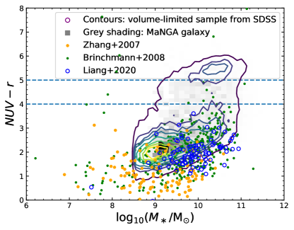
Figure 1: The color-mass diagram of the combined WR sample. We use $NUV-r$ color and stellar mass both based on elliptical Petrosian photometry from NSA catalog. The contours and the gray shading both represent the general population of galaxies. Contours show the number density of galaxy points on this diagram of a volume-limited sample selected from NSA catalog ($z<0.03$, $M_{\ast}>10^{8.5}\mathrm{M_{\odot}}$, $h=0.7$). Gray shading is MaNGA galaxies corrected by volume weights provided in Wake et al. (2017) so as for a volume-limited sample. Blue circles are WR galaxies from paper I and orange and green dots are WR galaxies of Z07 and B08 respectively. Cyan lines are empirical boundaries among the blud cloud, the green vallay and the red sequence of galaxies.

Based on the analyses of completeness of catalogs in Paper I, we now further discuss the physical parameter coverage of the three catalogs in Figure 1. Overall, as expected, the WR galaxies are found exclusively in strongly star-forming galaxies with bluest colors at their stellar mass. The galaxies from Z07 are systematically bluer and less massive than the MaNGA galaxies from Paper I, while the B08 catalog covers a wider range in both color and mass than the other two catalogs. The differences among the three catalogs reflect the selection biases in empirical searching for WR galaxies. Z07 required significant $EW(\mathrm{H\epsilon})$ emission and thus picked the most intense star forming regions. Paper I was based on the lower-order Balmer line $\mathit{\Sigma}(\mathrm{H\alpha})$ and thus the sample is dominated by more general star-forming galaxies, with the rare population of the Z07-type galaxies being barely included due to the small size of the parent sample. The B08 catalog mainly covers a similar area as the MaNGA WR catalog but it also extends to the regime of the bluest galaxies, thus it is most complete among the catalogs in terms of the global property coverage. This may be attributed to two factors: the fact that the B08 catalogs did not rely on high-order Balmer lines, and the much larger parent sample from which the B08 catalog was selected. Although small in galaxy number, the MaNGA-based catalog is unique for the many off-center WR regions that were missing in the SDSS-based catalogs.

2.2 Measuring the WR blue bump

For each of the 910 spectra in our catalog, we have performed full spectral fitting and measured the flux and equivalent width of the WR blue bump based on the starlight-subtracted spectrum. Our spectral fitting code was originally developed by Li et al. (2005) and further improved in Paper I. In short, we construct stellar templates by applying the technique of principle component analysis (PCA) to the MILES single stellar population (SSP) models (Vazdekis et al., 2010, 2015). The first nine eigenspectra produced by the PCA are adopted as fitting templates, and are used to fit the SDSS spectrum (for the WR galaxies from Z07 or B08) as well as the stacked spectrum of the WR region (for the WR regions from MaNGA). During the fitting, all significant emission lines as well as the wavelength range of the WR blue bump (4600-4750Å) are masked out. Apart from the continuum, we also obtain emission line measurements such as $F_{\mathrm{H\beta}}$ and $EW_{\mathrm{H\beta}}$ in this step. Details can be found in Li et al. (2005) and Paper I about the construction of the stellar templates and the scheme of masking emission lines.

For comparison of WR features with model predictions, it is important to reliably measure the profile of the WR bump, which is a combination of WR star-driven emission lines plus nebular emission lines that are irrelevant to the WR feature. Basically, the blue bump consists of the following WR features: He II $\lambda$4686, N V $\lambda\lambda$ 4605, 4620, N III $\lambda\lambda\lambda$ 4628, 4634, 4640 and C III/C IV $\lambda\lambda$ 4650, 4658. The nebular emission lines falling in the WR bump include: He II $\lambda$4686 (narrow line), [Fe III] $\lambda\lambda\lambda$4658, 4665, 4703, [Ar IV] $\lambda\lambda$4713, 4740, He I $\lambda$4713, [Ne IV] $\lambda\lambda$4713, 4725. Given the current spectral quality, it is not possible to accurately fit so many features independently. Based on Brinchmann et al. (2008) and Miralles-Caballero et al. (2014, 2016), and the occurrence of each feature and their relative strength, we have determined the following fitting procedure as well as initial guesses and fitting ranges of each parameter.

Starting from the residual spectrum of the full spectrum fitting, we first perform a linear fit to the two side windows at 4500-4550 Å and 4750-4800 Å, and calculate the root mean square ($RMS$) in the two windows. Then, we fit the following five features, each with a Gaussian: the He II bump centered at 4686 Å, the C and N bump at around 4645 Å, the He II $\lambda$4686 narrow line, the [Fe III] $\lambda$4658 narrow line, and the [Ar IV] $\lambda$ 4713 and He I $\lambda$ 4713 narrow line. During the fitting the Gaussian center of the He II bump and narrow lines are fixed at the known wavelength, while the center of the C and N bump is allowed to change, but limited to the range of $\lambda=4645\pm 7.5$ Å. Gaussian width $\sigma$ of narrow lines are fixed at the value of $\sigma_{\mathrm{H\beta}}$ while that of broad components are free parameters within the range $0-22$Å. This upper limit of 22 Å corresponds to the velocity dispersion (1425 km/s) of the WR wind, and this width is almost the largest possible value according to literatures on individual WR stars (e.g. Willis et al., 2004). The linear fit obtained in the first step is used as the baseline in this multi-Gaussian fitting and the $RMS$ is used to estimate the significance of emission features. We keep the bumps or lines if the flux from their Gaussian fit has a significance larger than 3. Next, if the width of the C and N bump around 4645 Å reaches the upper limit of 22 Å, another Gaussian is added to fit the broad component at 4612 Å. Finally, if the peak flux of the residual spectrum (with all the above fitted components removed) is larger than 4 times the $RMS$, a new Gaussian is added in the fitting, which is either a broad component if the peak occurs at $<4650$ Å or otherwise a narrow comopent. The step is iterated until all fluxes in the residual spectrum is lower than 4 times the RMS or at most three additional components are added in this step. The fitting procedure uses the python package PyAstronomy (Czesla et al., 2019).

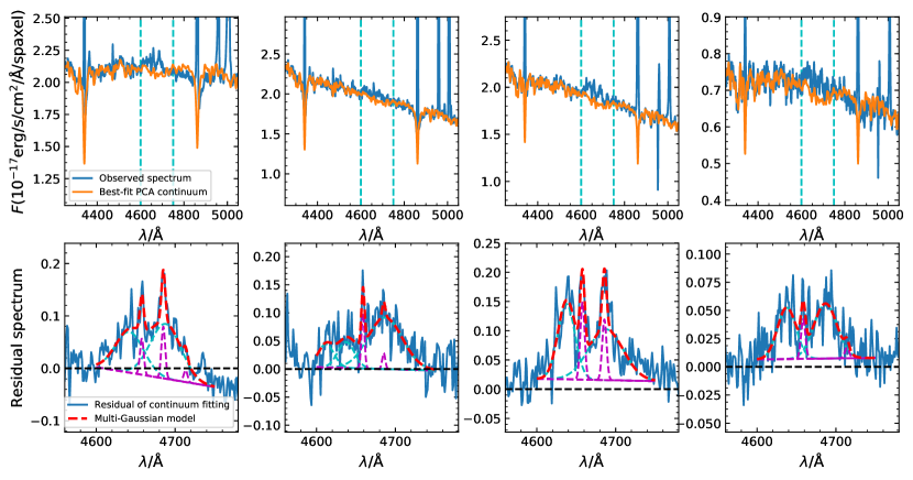
Figure 2: Four examples of the fitting to the WR blue bump. The upper panels show the observed WR spectra (in blue) and their full spectral fitting models (in orange) from PCA algorithm with MILES templates. The lower panels show the blue bump feature in the residual and zoom-in the WR window shown with the two vertical dashed lines in the upper panels. The two (or three) cyan lines are the C/N bump(s) (at $\sim 4645\mathrm{\AA}$) and the He II bump (at 4686Å) while the purple lines are narrow nebular emission lines. The red line is the superposition of all components.

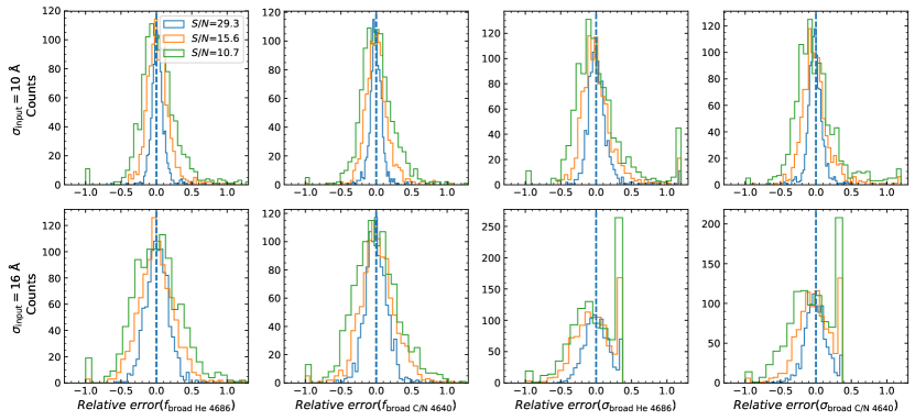
Figure 3: Simulation of the multi-Gaussian fitting to artificial WR blue bumps. We add random noise to artificial WR bumps and calculate relative error between the measured values from fitting and the input values. We perform this procedure for 1000 times for each input combination ($\sigma_{\mathrm{in}}$, broad emission $S/N$) and show the distribution. The upper panels have input Gaussian width of $\sigma=10$Å (for both the C/N and the He II bumps) while in the lower panels the two bumps each has width of $\sigma=16$Å. Different colors in each panel correspond to different broad emission $S/N$. In four columns, from left to right, we show the distributions for four measured parameters of the two broad emission lines: flux of the He II bump, flux of the C/N bump, width of the He II bump and width of the C/N bump.

Figure 2 shows an example of the Gaussian fits. The two (or three) Gaussians plotted in cyan are the C/N bump(s) around 4645 Å and the He II bump at 4686 Å, while the magenta curves are the narrow nebular emission lines. The red curve is the superposition of all the fitted components.

In order to test the reliability of our fitting. We have generated a set of mock spectra by artificially creating a WR blue bump with two different widths (Gaussian $\sigma$=10 Å and $\sigma$=16 Å) and including three different levels of uncorrelated Gaussian noise. Each spectrum includes two broad components (the C/N bump at 4645 Å and the He II bump at 4686 Å with equal flux and equal width of either 10 Å or 16 Å for different mock sets) and three narrow emission lines (He II $\lambda$4686, [Fe III] $\lambda$4658, [Ar IV] $\lambda$ 4713 and He I $\lambda$ 4713). We fit the mock spectra in the way described above and repeat the process for 1000 times for each mock bump with newly generated noise. In Figure 3, we show the distributions of the resulting relative error for the flux and width of the two broad components. We can see that, for He II and C/N bump fluxes, the relative difference between the input and output values is centred at zero, and shows a Gaussian-like distribution with a FWHM that ranges from $\sim 20\%$ at broad emission $S/N\sim 30$ to $\sim 50\%$ at $S/N\sim 10$. For the width of the two bump components, the overal distribution of the relative error is similar to that of the flux, but an apparent piling up is seen at the right-hand side, with stronger effect at lower $S/N$. This is a sign of the fitting hitting the upper boundary of the width before convergence probably due to noise. We check the fits for the real spectra and find such case indeed happens in some spectra. We visually examined these spectra and found they are fitted as well as other spectra. We understand this widening in the integrated WR emission as an effect of non-zero velocity dispersion of the targeted WR stellar population, for the adopted upper limit in fitting is based on individual WR stars. We also note that our results to be presented in the next section would not change if these cases were excluded from the analysis.

We should also mention that besides the blue bump, the red bump of broad emission lines around 5800 Å is also an important feature of extragalactic WR population (e.g. Crowther, 2007) and potentially sensitive to IMF variation (e.g. Guseva et al., 2000; Pindao et al., 2002). However, with current sensitivity of our data, detectable red bump features are only in a small fraction of WR regions. The occurrence and completeness of red bumps in our sample are rather small, mentioned in Paper I. Thus, we do not measure the red bump or compare it with model predictions. It is worth noticing that, however, the red bump (if existing) is indeed taken into account in our second approach which constrains the IMF models based on full spectral fitting (to be elaborated in subsection 2.5 and subsection 3.2), thus including all features that are sensitive to IMF variation.

2.3 Starburst99 model

Leitherer et al. (1999) publicized the online stellar evolutionary model Starburst99, based on the Leitherer & Heckman (1995) models. It incorporates a set of evolutionary model of different stars from zero-age main sequence to supernova explosion. It simulates the evolution of stellar parameters including mass, luminosity, effective temperature, surface chemical composition, etc and assign stellar spectra to obtain the synthesized total spectrum at each time slice given different physical conditions such as metallicity and the IMF. This model is designed for starburst or young stellar population. It is thus among the few models that incorporate WR population. Its WR feature is essentially the same as described in Schaerer & Vacca (1998).

The advantage of Starburst99 is the very fine time grids and a wide range of IMF slopes. WR population is very young and short-lived. Its lifetime is typically less than 10 Myr, which is by order of magnitudes smaller than normal stellar population. Starburst99 calculates stellar evolution by 0.1 Myr precision and thus provides 90 steps in the range of 1-10Myr. It provides complete sets of predicted WR feature parameters with IMF slope $\alpha=1.00,2.35,3.30$ and stellar metallicity $Z=0.0004,0.001,0.004,0.008,0.02(\mathrm{Z_{\odot}}),0.04$.

Besides different physical conditions, Starburst99 also allows for different star formation histories (SFHs). For $\alpha=2.35$, it provides model predictions with five different SFH — instantaneous burst and constant star formation of 1, 2, 10, 100 Myr.

2.4 BPASS model

In addition to Starburst99, we also use the latest stellar evolution model BPASS v2.2.1 (Stanway & Eldridge, 2018; Eldridge et al., 2017), which provides models for both singular stellar populations and binary stellar populations. This allows us to examine the effect of binary populations on WR features as well as the resulting constraints on the IMF slope. The effect could be significant. For instance, when binary evolution is considered, the lifetime of WR population can be extended from 5 Myr to 10 Myr (Eldridge & Stanway, 2009). BPASS adopts atmosphere models from Potsdam PoWR group (Hamann & Gräfener, 2003; Sander et al., 2015) and a distribution of binary parameters including binary fraction presented in the Table 13 of Moe & Di Stefano (2017), which were based on local stellar populations and lack information for sub-solar metallicity populations as a caveat.

BPASS has finer metallicity grids than Starburst99 but a narrower IMF slope range and coarser time grids. It provides complete sets of single stellar population spectra with 13 different metallicities from $Z=1.0\times 10^{-5}$ to $Z=0.040$, and three IMF slopes $\alpha=2.00,2.35,2.70$. it has two sets of models with an upper mass limit of $M\mathrm{{}_{upper}}=100\mathrm{M_{\odot}}$ and $300\mathrm{M_{\odot}}$. The time resolution is 0.1 dex and therefore has only 10 grids in 1-10 Myr. Unlike Starburst99, BPASS only provides instantaneous bursty models.

BPASS simple stellar population (SSP) models involve WR stellar emission lines when WR stars present. In order to compare the strength of the WR bump between model and data, we have measured the equivalent width of the blue WR bump of the SSP’s, adopting a local linear baseline. The WR bump exists only in very young populations so the stellar absorption lines are not abundant and the stellar continuum is rather flat (except for the oldest snapshot at $\log_{10}(Age)=7.5$ of $Z=0.02$ or higher, to be mentioned later). In the next subsection (subsection 2.5), we will also use these SSP models as templates to directly fit the spectra of WR galaxies/regions in our sample. This allows direct modeling of WR spectra with SSP’s.

2.5 Bayesian inference of WR spectra

In subsection 2.2 we have performed full spectral fitting to each of the 910 WR spectra in our sample, in order to separate emission lines (particularly the WR blue bump) from the stellar spectrum so that the WR bump can be reliably measured. Now we perform full spectral fitting to the WR spectra again, but using BIGS (Bayesian Inference for Galaxy Spectra), which is a Python spectral fitting code developed by Zhou et al. (2019). BIGS adopts the approach of Bayesian inference and Markov chain Monte Carlo algorithm to model the composite stellar populations (CSP) present in the observed WR spectra. The code incorporates different stellar population models and all IMF’s discussed in previous subsections. By comparing the Bayesian evidence for different models, one can make model selection reliably and efficiently. In subsection 3.2 we will take advantage of this virtue to compare BPASS models of different IMF’s.

The working process of BIGS can be summarized as follows. First, a stellar IMF and a specific star formation hisotry (SFH) are assumed. The SFH model is then combined with a set of SSP templates of BPASS and a simple screen dust model (Charlot & Fall, 2000) to generate composite model spectra, which are then convolved with the stellar velocity dispersion derived above (subsection 2.2) to account for kinematic and instrumental broadening effects. Next, the model spectra are compared with each of the observed spectra, and accordingly the likelihood for a given set of model parameters is calculated. The MULTINEST samplper (Feroz et al., 2009, 2013) is utilized to sample the posterior distributions of the model parameters and derive the Bayesian evidence. The BIGS code has been successfully appiled to MaNGA data to constrain the IMF slope for ellitpical galaxies (Zhou et al., 2019), as well as SFHs of both low-mass galaxies (Zhou et al., 2020b) and massive red spiral galaxies (Zhou et al., 2020a).

We have fitted each of the WR spectra using BIGS. Specifically, the WR population is modeled by a recent nearly-instantaneous burst with lookback time 0-10 Myr , later referred to as the “bursty stellar population”. This component is superposed to an underlying old stellar population modelled by the commonly-adopted exponential $\tau$-decaying model. Free parameters in fitting are dust attenuation quantified by color excess $E(\mathrm{B-V})$, burst-to-total mass ratio $f$, stellar metallicity of the bursty stellar population $Z_{\mathrm{b}}$, standard parameters of the $\tau$ model (i.e. stellar metallicity $Z_{\tau}$, lifetime $\tau$, and starting time $t_{0}$). The two metallicities $Z_{\mathrm{b}}$ and $Z_{\tau}$ are fitted independently in the fitting. We take the best-fit metallicity of the bursty stellar population as the metallicity of the WR population (for simplicity, we define $Z\equiv Z_{\mathrm{b}}$ hereafter), and use it for all following figures and discussion. We note that we have dropped a few spectra with unreasonably low metallicity in the tail of the derived $Z$ distribution ($\log_{10}(Z/\mathrm{Z_{\odot}})<-1.5,\ \mathrm{Z_{\odot}}=0.02$). During the fitting we have masked out emission lines in a iterative manner (see Li et al., 2005, for details), but the WR bump is kept and fitted.

For each spectrum, we have done multiple fittings using all the available SSP templates from BPASS. These include two sets with different types of evolution (i.e. singular and binary), and each set consists of nine SSP models with different IMF assumptions (corresponding to four different high-mass slopes paired with two different upper mass limits, plus an additional Salpeter IMF; see Table 1 for details). As a result, for each WR spectrum, we have 18 fittings and correspondingly 18 derivations for each aforementioned physical quantity such as $E(\mathrm{B-V})$, $Z$, etc. Figure 4 shows the cumulative distributions of the measurements of the stellar metallicity (the bursty stellar population), with solid (dotted) lines for the singular (binnary) population models and different colors for the different IMF’s, as indicated. We have scaled the $Z$ measurements of each WR spectrum by the measurement of an arbitrarily chosen model, which is the singular model with a Chabrier IMF and an upper mass limit of 100 M_⊙. Overall, as one can see, different models give rise to similar distributions of $Z$, as indicated by the sharp rise at around $Z/Z_{\mbox{chab,100,singular}}=1$ and the relatively narrow range of the median $Z$ (indicated by the horizental dotted line) spanned by the models. The largest difference between binary models and this particular singular model, which is $\begin{subarray}{c}+0.31\ \mathrm{dex}\\ -0.06\ \mathrm{dex}\end{subarray}$, occurs with the binary model of $\alpha=2.70$ and $M_{\mbox{upper}}=100\ \mathrm{M_{\odot}}$ (the dotted brown line) and the binary model of $\alpha=2.00$ and $M_{\mbox{upper}}=300\ \mathrm{M_{\odot}}$ (the dotted orange line). The differences are smaller if the comparison is limitted to the singular population models only, with the larggest difference ($\lesssim 20\%$) occuring between the same pair of models. Apart from looking at the median values, the smaller differences between the singular models can also be seen from the more sharply rising of the distributions. These results indicate that the $Z$ measurements are weakly dependent on the adopted IMF’s, but there are systematic differences betweeen the singular and binary models for a given IMF. In what follows, we will need to divide our WR galaxies/regions into subsets according to stellar metallicity. For simplicity, we use the median measurement of $Z$ for each WR galaxy/region, but separately for the case of singular and binary population models.

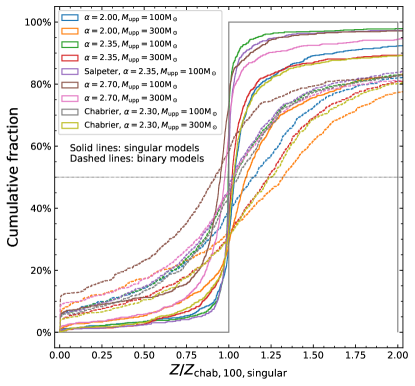
Figure 4: The comparison of derived bursty metallicity among different IMF assumptions. Each WR spectrum has a set of derived $Z$’s from fitting with different IMF assumptions. We arbitrarily set the singular model of Chabrier IMF with 100 M_⊙ upper limit to be the standard and divide all other metallicity values of each spectrum by its $Z_{\mbox{chab,100,singular}}$. We then plot the cumulative distribution of the ratios. The gray line of Chabrier IMF with 100 M_⊙ upper limit is, by construction, entirely 1.00. The horizontal dotted line crosses each cumulative distribution at its median value.

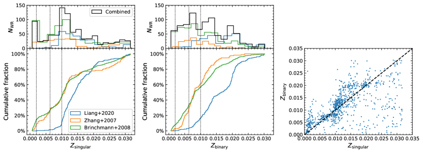
Figure 5: The distribution of the combined WR sample in $Z$. The histogram (number of WR spectra or regions $N_{\mathrm{WR}}$) and cumulative distribution of $Z$ derived from sigular (binary) model fitting is shown in the left (middle) panel. Different colors indicate different WR catalogs. See subsection 2.5 for details in derivation of $Z$. Vertical dotted lines show the boundaries of our four $Z$ bins used in Figure 6 and Figure 7. We set the bin boundaries according to the availability of $Z$ grids in Starburst99 models and BPASS models. In the right panel, we show the scatter plot of $Z_{\mbox{singular}}$ and $Z_{\mbox{binary}}$. When Z07 and B08 are plotted individually, they both have their original full catalogs while in the combined distribution (black histograms) and the scatter plot (right panel), their common 101 galaxies only appear once.

Figure 5 displays the distribution of the median stellar metallicity mesurements for the singular population models (left panel) and the binary population models (middle panel). The main panels show the cumulative distribution functions, while the upper panels show the corresponding histograms. Results for the three WR catalogs are shown separately. The overal distribution of all the WR galaxies/regions in our sample is plotted as the black histogram in the upper panels. When Z07 and B08 are plotted individually, they both have their original full catalogs while in the combined distribution (black histograms) and the scatter plot (right panel), their common 101 galaxies only occur once. Our sample spans a wide range of metallicity (from Z$\sim$0.001 up to Z$\sim$0.03), as one can see from the figure. The Z07 and B08 catalogs present similar distributions in $Z$, while the WR catalog from MaNGA is relatively metal-rich. This might be implying that the WR regions at galactic centers as selected by Z07 and B08 are more metal-poor than those in the disk which dominate the WR catalog selected from MaNGA. We will come back to this point in a later paper of this series (Liang et al. in prep.). The vertical dotted lines in the left and the middle panels indicate the boundaries used to select subsamples in subsection 3.1 for Figure 6 and Figure 7. We set the bin boundaries according to the availability of $Z$ grids in Starburst99 models and BPASS models. The right panel compares the median measurements for the singular and binary population models. Most data points distribute along or closely to the identity line, while a considerable fraction of the data points deviate from the line. This means the choice of using singular evolution model or binary evolution model can cause a significant difference in the derived metallicity to a small fraction of observed spectra. This further suggests it is necessary to consider the effect of binary populations when modelling the underlying stellar populations of observed spectra.

In Table 1, we summarize key information of our modeling described in this section.

Table 1: A table summarizing all models.

		Singular modeling		Binary modeling
		Starburst99	BPASS singular	BPASS binary
Model feature	IMF Slope $\alpha$	1.00, 2.35, 3.30	2.00, 2.30, 2.35, 2.70	2.00, 2.30, 2.35, 2.70
	IMF upper cutoff $M_{\text{upper}}$ in M⊙	120	100, 300	100, 300
	Metallicity $Z$ grids	4E-4, 1E-3, 4E-3, 8E-3, 0.02 0.04	13 grids from 1E-5 to 0.04	13 grids from 1E-5 to 0.04
	Number of age grids in 0-10 Myr	90	10	10
Employment in this paper	Use as SSP templates in BIGS fitting	No	Yes	Yes
	Use in $Z_{\text{WR}}$ derivation	No	Yes, $Z_{\text{singular}}$	Yes, $Z_{\text{binary}}$
	Use in WR property comparison in §3.1	Yes	Yes	Yes
	Use in Bayesian inference of IMF slope in §3.2	No	Yes	Yes

3 Constraining the high-mass slope of the IMF

3.1 Constraining the IMF slope with SSP’s

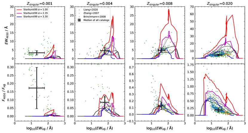
Figure 6: We compare WR parameters of the observation and the singular evolutionary model (namely Starburst99) in this figure. The upper four panels show comparison in the plane of $EW_{4650}$ vs log($EW_{\mathrm{H\beta}}$) while the lower four panels show $F_{4650}/F_{\mathrm{H\beta}}$ vs log($EW_{\mathrm{H\beta}}$). WR regions (shown as dots) are divided into four $Z$ bins (four different columns) and compared with corresponding model predictions (shown as evolutionary tracking lines). The large black cross is the median value of data points in each panel with errorbars showing median absolute deviation. Different colors of lines are different IMF assumptions with the red line being the steepest IMF slope ($\alpha=3.30$) and the blue line being the flattest slope ($\alpha=1.00$). The gray lines are assuming the same IMF slope as the megenta line ($\alpha=2.35$) but assuming more extended SFH than colored lines of instantaneous starburst. The darker the gray, the more prolonged the SFH.

First, following Z07, we examine the correlation of IMF slope with stellar metallicity by comparing the observed WR features in our sample with that of the SSP’s from Starburst99, using WR galaxies/regions in different stellar metallicity intervals. The results are shown in Figure 6 where we plot the distribution of $EW_{4650}$ (upper panels) and $F_{4650}/F_{\mathrm{H\beta}}$ (lower panels) versus $EW_{\mathrm{H\beta}}$. The measurements of $EW_{4650}$ and $F_{\mathrm{H\beta}}$ are obtained in subsection 2.2, while $F_{\mathrm{H\beta}}$ and $EW_{\mathrm{H\beta}}$ are described in subsection 2.1. As pointed out in Z07, the use of $EW_{4650}$ and ratio to $\mathrm{H\beta}$ can alleviate the uncertainties from dust extinction. In the figure, panels from left to right correspond to four metallicity ranges: $Z<0.002$, $0.002<Z<0.0063$, $0.0063<Z<0.01$, and $Z>0.01$. The median metallicity of the observed galaxies/regions in each bin is $Z=0.0013$, 0.0045, 0.0089, 0.0150 in case of singular models, and $Z=0.0012$, 0.0043, 0.0079, 0.0152 in case of binary models. In each panel the small points represent WR galaxies or regions from our combined sample, and the big cross and the error bar indicate the median of the data points and the median of the absolute deviation from the data’s median. We use the median of data points and the median absolute deviation, instead of the mean average and the standard deviation as often adopted, in order to minimize the effect of outlier data points.

For comparison, predictions of evolutionary tracks of instantaneous starbursts from Starburst99 with metallicity of $Z=0.001$, 0.004, 0.008, 0.020 are plotted as colored lines in the four panels. In each panel, lines of different colors represent the three different IMF slopes: $\alpha=1.00$, 2.35, 3.30. As one goes from low to high metallicities, the location of the data points move significantly with respect to the model lines. As a result, models of different IMF slopes are needed to interpret the data at different metallicities. In the lowest metallicity bin ($Z=0.001$), all the data points are far beyond the enclosed parameter range of all the models. At $Z\sim 0.004$, quite a fraction of the data points as well as the median value fall in between the red ($\alpha=1.00$) and magenta ($\alpha=2.35$) lines. At $Z\sim 0.008$, more data points fall below the magenta line, and the median of the data points fall slightly below the blue line ($\alpha=3.30$). Finally, in the highest metallicity bin where $Z=0.02$, the majority of data points and their median value are well enclosed by the model with the steepest IMF (blue line, $\alpha=3.30$). These clearly suggest a metallicity-depdent IMF slope in the sense that the IMF steepens with increasing metallicity. From the figure, as one can see, this trend is attributed to the significant change of the model tracks with metallicity in contrast to the weak metallicity-dependence of the distribution of the data points in the two parameter diagrams. In all panels, the median of $EW_{4650}$ remains $\sim$5Å, while the median of $F_{4650}/F_{\mathrm{H\beta}}$ spands a limited range of $0.12-0.18$. In the models, however, for a fixed IMF slope both $EW_{4650}$ and $F_{4650}/F_{\mathrm{H\beta}}$ change significantly with metallicity. Taking the megenta line ($\alpha=2.35$) for example, the peak value of $EW_{4650}$ increases from $\sim$5Å at $Z=0.001$ to $\sim$28Å at $Z=0.02$, and the peak value of $F_{4650}/F_{\mathrm{H\beta}}$ increases from $\sim 0.02$ to $\sim 0.85$. Combining the observational (lack of) trend and the theoretical trend, one can clearly conclude that any single IMF cannot explain the data at all metallicities, and that a “bottom-heavy” (“top-heavy”) IMF is needed to interpret the data at high (low) metallicites. This result is well consistent with Z07 and recent studies which use different catalogs/data and methods (e.g. Cappellari et al., 2012b; Li et al., 2017; Parikh et al., 2018; Zhou et al., 2020b).

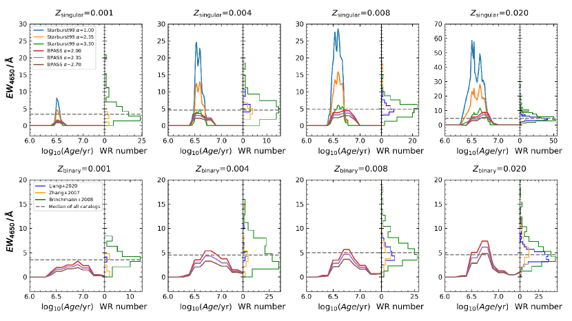
Figure 7: The evolution of WR parameters in singular evolution models (upper panels) and binary evoluiton models (lower panels). Different colunms are for different $Z$ bins. In each panel, the main sub-panels on the left show model predictions from Starburst99 and BPASS with different colors indicating different IMF’s, and the side panels on the right show the histograms of observed $EW_{4650}$ of WR spectra in respective $Z$ bins. The horizontal dashed lines is the median value of the combined WR sample in each $Z$ bin. Note that the slight rise of model lines towards $\log_{10}(Age)=7.5$ is an artifact due to linear fitting on BPASS SSP’s where absorption lines prevail.

In addition to the instantaneous burst models, we also consider model predictions from Starburst99 for star formation with longer durations. We show the results in Figure 6 for the Salpeter IMF ($\alpha=2.35$) as different shades of gray lines in each panel. The four lines from light gray to dark gray correspond to SFHs with duration $t=1,2,10,100$ Myr. As the burst duration increases, the predicted WR bump becomes weaker when compared to $\mathrm{H\beta}$ emission. This can be explained by the different lifetimes between the WR population (which produce the WR feature at around 4650Å) and other OB stars (which produce the $\mathrm{H\beta}$ emission). For an instant starburst of given IMF and metallicity, WR stars and OB stars are formed at the same time and mixed instantaneously, and the WR feature is relatively strongest in this case. For an extended burst, since WR stars have shorter lifetimes than other OB stars, at any given time the existing WR population is mixed with both contemporary OB stars and those fromed at earlier times. This dilutes the feature of WR stars against the continuum (the denominator of $EW_{4650}$) and the $\mathrm{H\beta}$. In Figure 6, we can see gray lines basically span the parameter space between the megenta lines and the blue lines. Thus, variation in SFH alone cannot fully interpret the data when the IMF slope is fixed at $\alpha=2.35$.

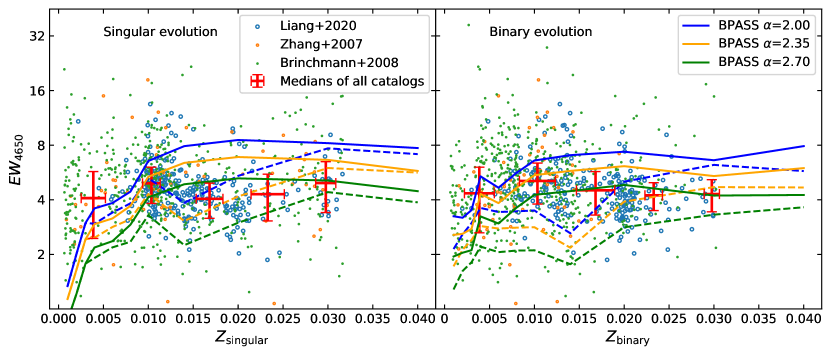
Figure 8: Comparison of $EW_{4650}$ and $Z$ for both singular evolution (left) and binary evolution (right). Different colored lines are model predictions with different IMF slopes. Since it is impossible on this 2D figure to show another dimension of time evolution of $EW_{4650}$, we instead show the maximum values during the WR phase with solid lines and the median values of $EW_{4650}$ (among snapshots when significant WR feature exists) with dashed lines. Red crosses are median value of the data points at different $Z$ bins. Errorbars are median absolute deviation.

Next, in Figure 7, we show the evolution of the WR parameter $EW_{4650}$ with time as predicted by BPASS for both singular populations (upper panels) and binary populations (lower panels), and for different IMF slopes (different lines) and metallicities (different columns). For the singular populations, the predictions of Starburst99 are also plotted for comparison. From the observational side, we have obtained measurements of $EW_{4650}$ for all the WR galaxies and regions. However, it is hard to reliably estimate ages for such young stellar populations, considering the age-metallicity degeneracy and uncertainties in the age derived from stellar population synthesis. Also, the star formation history we use in subsection 2.5 does not set the age of the starburst as a free parameter. Therefore, we plot the histograms of $EW_{4650}$ of the WR galaxies/regions in side panels, with the median value indicated by the horizontal dashed lines. As one can see from the upper panels, although the stellar ages from the two models cover similar ranges, the WR features from Starburst99 are much stronger than that from BPASS for given IMF and metallicity. Despite the discrepancy in the absolute value of $EW_{4650}$, the two models predict the same trend that, at fixed IMF slope, $EW_{4650}$ increases with increasing metallocity. Since the median value of $EW_{4650}$ in the sample depends very weakly with metallicity, both models requires an increase in IMF slope as one goes from low to high metallicity in order to bring the mdoels better match the data. For instance, the model of Starburst99 with $\alpha=2.35$ matches the data in the lowest metallicity bin, while the model with $\alpha=3.30$ is most compatible to the data in the highest metallicity bin. In case of BPASS, all the models are much lower than the data in the lowest metallicity bin, which may be attributed to the limited range of IMF slope in the model ($\alpha=$2.00-2.70). Models of $\alpha=2.00$ get closer to the data in the two intermediate metallicity bins, while the model of $\alpha=2.70$ best matches the data in the highest metallicity bin.

In the lower panels, the need of steeper IMF’s at higher metallicities can also be seen for the binary population models. In the lowest metallicity bin, the model with the flatest IMF ($\alpha=2.00$) matches the median of the sample, while in the two intermediate metallicity bins the data falls in between the models with $\alpha=2.00$ and $\alpha=2.35$. In the highest metallicity bin, it is the model with the steepest IMF ($\alpha=2.70$) that best matches the data. This result suggests that the metallicity-dependent variation of the IMF slope holds in both singular population models and binary population models.

The difference caused by varying between $M\mathrm{{}_{upper}}=100\ \mathrm{M_{\odot}}$ and $M\mathrm{{}_{upper}}=300\ \mathrm{M_{\odot}}$ (with other parameters fixed) is tiny. Thus, for simplicity we do not differentiate this upper mass limit, where relevant.

In Figure 8 we plot $EW_{4650}$ as a function of stellar metallicity, for both the data and model predictions. We consider BPASS models of both singular (left panel) and binary (right panel) populations. Galaxies/regions from our sample are plotted in small dots, while the red crosses and erorbars represent the median and the median absolute deviation in a given metallocity bin. For given IMF and metallicity, we show both the peak value of $EW_{4650}$ (with solid lines) as well as the median value (with dashed lines) among snapshots when significant WR feature exists (more specifically, the median value among SSP’s with at least 10% of the peak value, which is a reasonable threshold considering the observed $EW_{4650}$ range). Overall, as already seen from previous figures, the median observed $EW_{4650}$ shows weak dependence on metallicity in the data. In the models, with fixed IMF slope the predicted $EW_{4650}$ increases with increasing metallicity, and the effect is most remarkable at lowest metallicities ($Z\lesssim 0.01$). At higher metallicities, the predicted $EW_{4650}$ flattens out. Combining the weak varation (or no variation) of the observed $EW_{4650}$ at all $Z$’s and the significant increase of the model-predicted $EW_{4650}$ as a function of $Z$ assuming a fixed IMF, one can expect that we need different IMF assumptions at different $Z$’s in order to reproduce observed values at all $Z$’s. More specifically, we need to assume a flatter IMF (i.e. “top-heavy”) at lower metallicities and a steeper IMF (i.e. “bottom-heavy”) at higher metallicities.A more detailed comparison between data and model is following, which leads to this IMF variation in a more quantitative way.

When comparing observed data points with models in Figure 8, one needs to compare the data points with the intervals spanned between peak values and median values at any given IMF. Since the ages of observed WR regions are unknown, different WR regions should be at randomly different phases of WR lifetime. Thus, observed WR sample should have a distribution (rather than an exact value) of $EW_{4650}$ at any given $Z$ bin. Besides, the detection completeness of WR regions is higher for regions with higher $EW_{4650}$, since these bumps are less likely to be destroyed by observational noise in the spectra. Combining the above analysis, we expect the detected WR $EW_{4650}$ should mostly fall in this interval (between medians and peaks of model prediction). In the upper panel, the median observed $EW_{4650}$ shown with red crosses fall in (or are closer to) the blue interval alone ($\alpha=2.00$) at low $Z$ while they fall in the green interval alone ($\alpha=2.70$) at high $Z$. In other words, it is clear a universal IMF does not exist to encompass WR observations at all metallicity. In the right panel of binary modeling, this trend also exists but is less clear. The red cross at the lowest $Z$ falls in the blue interval ($\alpha=2.00$) but is also at the boundary (peak) value of the orange interval ($\alpha=2.35$), which means the flattest IMF slope is slightly preferred in this metallicity. The orange interval also encompasses the red crosses in the three intermediate $Z$ bins. In the highest $Z$ bin, the red cross falls below the orange interval and is at the boundary (peak) of the green interval ($\alpha=2.70$). Thus, the steepest IMF is slightly preferred at the highest $Z$. It is interesting that the same trend holds in both singular and binary population models, although the metallicity dependence of the WR featuer in the binary models is slightly weaker than that in the singular models.

It has been seen that for a given IMF slope, models predict stronger WR emission (higher $EW_{4650}$) at higher metallicity. This is due to the positive correlation between metallicity and the mass loss rate (and therefore stellar wind emission) of WR stars (Crowther, 2007). The absence of such trend in observed WR population means at lower metallicity, more WR stars are needed to compensate for their relatively weaker stellar winds than at high metallicity. This immediately implies a “top-heavy” IMF at low metallicity.

We should stress that all these analysis should be considered in a statistical manner. In other words, we always compare the average of data points with models. If we examine individual data points, we can see many of them locate well apart from any model prediction, especially at the low metallicity end. The discrepancy at low metallicity is very large for singular evolution case, e.g. in the bottom-left panel of Figure 6, the upper-left panel of Figure 7, and the leftmost part of the left panel of Figure 8. The introduction of the binary evolution models alleviate this discrepancy, which should be a demonstration of the importance of binary evolution. Nonetheless, even when we look at the binary case, some individual points still deviate from all model predictions. This can be attributed to uncertainties in measuring WR bumps, the relatively narrow range of available IMFs in BPASS models, lack of knowledge in high-mass stellar evolution at low metallicity, etc. We leave deeper investigation of the discrepancy between models and individual WR regions to future studies.

3.2 Bayesion inference of the IMF slope from full spectral fitting

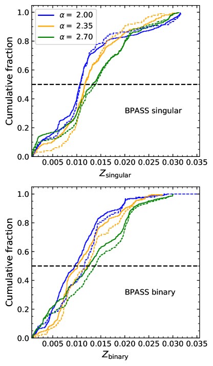
Figure 9: Cumulative distribution of $Z$ for WR sample grouped by their optimal IMF slope determined from Bayesian evidence of fitting. The upper panel is the singular fitting result and the lower panel is the binary result. Colored dashed lines are high spectral $S/N$ (at $\sim 4675\,\mathrm{\AA}$) subsamples of corresponding solid lines. Horizontal black dashed lines cross the colored lines at their median values.

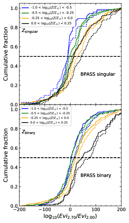
Figure 10: Cumulative distribution of Bayesian evidence ratio $\mathrm{log}_{10}(Evi_{2.70}/Evi_{2.00})$ for sub-samples grouped by $Z$. For each WR spectrum, since we have fitted it multiple times with different IMF assumptions, we now extract the Bayesian evidence of fitting with $\alpha=2.70$ IMF (i.e. $Evi_{2.70}$) and with $\alpha=2.00$ IMF (i.e. $Evi_{2.00}$) and take the ratio to indicate the preference between the two IMF slopes. The upper panel is from fitting with singular templates while the lower panel is from binary templates. Colored dashed lines are subsamples of corresponding solid lines with high $S/N$ (at $\sim 4675\,\mathrm{\AA}$). Horizontal black dash lines cross the colored distribution lines at their median values.

As described in subsection 2.5, we have performed full spectral fitting to each of the WR spectra in our sample using BIGS, which provides Bayesian evidence for us to select the best model among many others. We consider the BPASS models of both singular and binary populations. For each spectrum, we fit it with BIGS, using models of the three different IMF slopes: $\alpha=2.00$, 2.35 and 2.70. We then select one of the three IMF slopes which leads to the highest Bayesian evidence as the optimal IMF slope for the spectrum. In this way we divide the 910 WR galaxies/regions into three groups according to the optimal IMF slope. Figure 9 displays the cummulative distribution of $Z$ for the three groups. The upper and lower panels show results (solid lines) for the singular and binary models separately. In both panels, the metallicities of the group with the steepest IMF ($\alpha=2.70$, green lines) are higher than those of the other two groups, as can be seen from the separation between the distributions as well as the median metallicities indicated by the horizontal line. The separation between the distributions is apparent at $0.01<Z<0.02$. We note the curves converge at $Z<0.01$ and $Z>0.02$. We suspect this is possibly due to the narrow range of available $\alpha$ in BPASS. This narrow range of variation makes model less distinguishable at either very low ($Z<0.01$) or very high ($Z>0.02$) metallicity. This convergence may also be attibuted to lack of binary templates, since we can see in the lower panel the separation among curves are generally larger at the high-$Z$ end. We also select a subset of spectra with relatively high spectral signal-to-noise at $\sim 4675\,\mathrm{\AA}$ ($S/N>20$) and plotted the results as dashed lines in the same figure. Results of the high-S/N spectra are similar to those of the full sample with separation being slightly clearer in the binary modeling (lower panel).

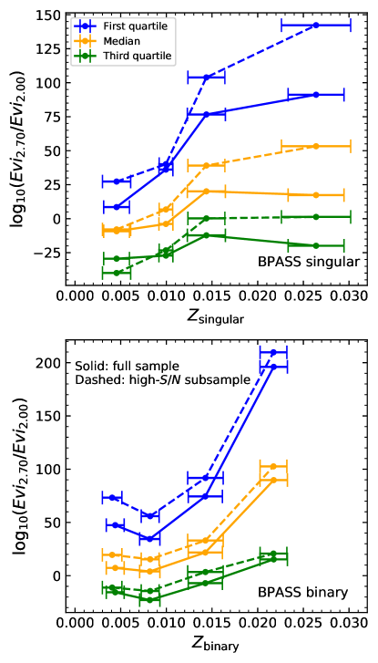
Figure 11: Evidence ratio $\mathrm{log}_{10}(Evi_{2.70}/Evi_{2.00})$ vs metallicity $Z$. We divide our sample into the same four $Z$ bins as used in Figure 10. At each $Z$, we show the three quartiles of evidence ratios in different colors. The solid lines are quartiles of the full WR sample while the dashed lines show those of a high-spectral-$S/N$ subsample. The horizontal error bars are the median absolute deviation of $Z$ in each bins.

In Figure 10, we divide all the WR galaxies/regions into four bins according to $Z$ specified in the legends. For each spectrum, since we have performed multiple fittings with different IMF assumptions, we now extract the Bayesian evidence from fittings with $\alpha=2.70$ and with $\alpha=2.00$. We calculate the ratio of them to indicate the preference between the two IMF’s. For each WR spectrum, if the ratio is larger (or smaller) than one, $\alpha=2.70$ (or $\alpha=2.00$) is favoured. We then plot the cummulative distribution of the Bayesian evidence ratio $\mathrm{log}_{10}(Evi_{2.70}/Evi_{2.00})$. Again, we show results for both the full sample (solid lines) and the subset with high spectral $S/N$ at $\sim 4675\,\mathrm{\AA}$ (dashed lines). Note that the four $Z$ bins in this figure as well as in the following figure are different from those in the previous subsection. In the previous subsection, the bins are set by the availability of $Z$ grids of model SSP’s, especially limited by the scarce grids of Starburst99 model. In this subsection, since we use Bayesian evidence to infer the IMF slope instead of comparing to SSP’s, we can better bin our sample by $Z$ into subsamples with roughly equal sizes. Also, we eliminate spectra with $Z<0.002$, for we have shown in the previous subsection that no model matches data well in this lowest $Z$ bin. Both the overall distribution and the median value of the evidence ratios favor larger values with increasing metallicity, especially for the subsample of high spectral $S/N$. This indicates that a steeper ($\alpha=2.70$) IMF is preferred at higher $Z$. This result holds for both singular and binary models.

In Figure 11, we further present the evidence ratios in a slightly different way from Figure 10. We divide our sample into the same $Z$ bins (with dots located at median $Z$ of each bin and median absolute deviation as error bars) and show quartiles of evidence ratios in each bin. In general, we can see a positive trend between evidence ratio quartiles (all of the three quartiles) with $Z$ in both panels (both singular case and binary case). In other words, at higher $Z$, the evidence ratios are higher no matter which quartile of the distribution we look at. This again indicates the steeper IMF $\alpha=2.70$ is preferred at higher $Z$, consistent with previous findings. The high spectral $S/N$ subsample results (shown with dashed lines) present a clearer trend in the singular modeling (upper panel) than the full sample (shown with solid lines) while in the binary modeling (lower panel) they are roughly the same as the full sample. Besides, the trend of singular (binary) modeling exists in lower (higher) $Z$ bins, i.e. $Z\lesssim 0.015$ ($Z\gtrsim 0.007$) and flattens out elsewhere. This means the transition between $\alpha=2.00$ and $\alpha=2.70$ happens at slightly different $Z$ intervals with singular and binary modeling. Besides, when we inspect the values of the evidence ratios instead of the trend, we find the singular modeling experiences a transition from negative median $\mathrm{log}_{10}(Evi_{2.70}/Evi_{2.00})$ to positive median values while the median values in binary modeling are positive at all $Z$. Although this phenomenon does not conflict with the variation of IMF given the clear trend of evidence ratio we have discussed, further studies are needed to better investigate the implied degeneracy between binary modeling and IMF variation. In addition, evidence ratios at the highest $Z$ bin have a larger variation reflected by the larger separation between the first and the third quartiles at this $Z$. The origin of this larger scatter is still unknown. We also notice the significant difference between median $Z_{\mathrm{singular}}$ and $Z_{\mathrm{binary}}$ in the highest $Z$ bin despite the same binning boundaries. This is a direct result of the systematically different distributions of $Z_{\mathrm{singular}}$ and $Z_{\mathrm{binary}}$.

To sum up, we have echoed our findings in subsection 3.1 by means of Bayesian inference of WR spectra in this subsection. A “top-heavy” IMF is preferred in low $Z$ environments. This holds for both singular modeling and binary modeling. A high spectral $S/N$ (at $\sim 4675\,\mathrm{\AA}$) subsample sometimes shows this trend more clearly than the full sample, namely in the lower panel of Figure 9, in Figure 10 and in the upper panel of Figure 11 . Nonetheless, we can see limitations of the narrow IMF slope range of BPASS models. Models covering wider ranges in $\alpha$ are needed in order to better constrain the relationship between $Z$ and $\alpha$, at both high and low metallicities.

4 Discussion

4.1 WR spectra as a unqiue probe of the IMF slope

WR spectra provide a unique probe to constrain the massive end of the IMF with the youngest stellar population ($<10\ \mathrm{Myr}$) in galaxies. This approach relies on the fact that the WR feature in integrated spectra of galaxies or star-forming regoins is produced by living massive stars during their WR phase, thus sensitive to the IMF slope at the high-mass end. This approach is complementary to other probes that have mostly focused on old stellar populations in early-type galaxies or bulges in late-type galaxies (e.g. Cappellari et al., 2012a; Li et al., 2017; Parikh et al., 2018; Zhou et al., 2019).

In an early work, Guseva et al. (2000) analyzed long-slit spectra of 39 WR galaxies covering a wide range of gas-phase metallicity. It was found that, at the lowest metallicites of their sample, the distribution of galaxies on the diagram of WR bump equivalent widths versus $EW_{\mathrm{H\beta}}$ can be better (though not fully) matched by theoretical predictions of the models of Schaerer & Vacca (1998) if a very shallow IMF with $\alpha=1.00$ is adopted instead of the Salpether IMF with $\alpha=2.35$. Though the original authors did not attribute this phenomenon to IMF variation. Based on the SDSS/DR3, Zhang et al. (2007) identified a large sample of 174 WR spectra and examined both $EW_{4650}$ and $F_{4650}/F_{\mathrm{H\beta}}$ as a function of $\log_{10}(EW_{\mathrm{H\beta}})$. The authors compared the WR galaxy distribution on these diagrams, for four different metallicity ranges separately, with predictions of the single population models of Schaerer & Vacca (1998) with different IMF slopes (the same models as used in Starburst99). This analysis led to the conclusion that steeper IMF slopes are needed at higher metallicities in order for the model to better match the data, in good agreement with the early hint from Guseva et al. (2000). The same trend is also seen in our work, as shown in Figure 6, but our work has well extended the work of Zhang et al. (2007) in the following aspects.

First, we have significantly enlarged the WR sample and improved the coverage of galaxy properties for the sample, by combining the SDSS-based WR catalogs constructed in previous studies (Zhang et al., 2007; Brinchmann et al., 2008) with the MaNGA-based catalog constructed in our previous work (Liang et al., 2020). As shown in Figure 1, different WR catalogs cover basic galaxy parameters in quite different ways, due to different selection methods. In addition, the SDSS spectra are limited to central regions of galaxies, and the MaNGA datacubes include outer regions of galaxies in our analysis. The combined sample thus includes a more complete set of WR regions from different locations and in differen types of galaxies.

Second, for consistency, we have used our own pipeline to re-analyze all spectra in the combined WR sample, instead of taking values from literature. We have carefully decomposed and measured the emission lines in the WR wavelength window. We have also applied our spectral fitting code BIGS which allows statistical comparison and selection of different models in a Bayesian inference framework. These careful treatments on data analysis have provided a solid basis to support our conclusions.

Thirdly, on the theoretical side, we have considered not only the singular evolution model as used in Zhang et al. (2007), but also the recently-developed model BPASS. The metallicity-dependent IMF slope variation is also supported by this new model. In addition, the binary population models in BPASS have allowed us to examine the effect of binary evolution. At intermediate-to-high metallicities, we find similar results when considering binary population models. At the lowest metallicities, models with binary populations predict larger equivalent widths of the blue WR bump, thus more closely matching the data than the singular population models. As can be seen in Figure 8, the binary model with the shallowest IMF well matches the median $EW_{4650}$ of the data at the lowest metallicities, while all the sigular models significantly underpredict the same quantity. This is the first time that binary evolution is explicitly considered in the constraint of the IMF.

4.2 Systematics and caveats in interpreting the results

Several sources of uncertainties and random error could have come into our analysis. First, we rely on stellar continuum subtraction in measuring WR features. This can cause some uncertainties in our measured $F_{4650}$ and $EW_{4650}$, due to residual continuum, in addition to the random error due to spectral noise. Second, in the derivation of metallicity of our spectra, we assume a two-component star formation history when carrying out stellar population synthesis. This is another souce of model-dependency. Again, we stress that given these uncertainties, we do not analyse any single WR spectra. All our results are based on a large sample, which should be more robust against uncertainties.

We mainly test two potential systematics. The first is contamination of WR stellar population by other populations, such as old underlying population and diffuse ionzed gas (DIG) surrounding WR pupulations. In principle, our second approach discussed in subsection 3.2 is not affected by this contamination, for we have already included and then subtracted the contribution of old populations to the spectra. However, this can affect our measured $EW_{4650}$ since the old population can contribute considerably to the stellar continuum. We select a subsample with the highest surface brightness (SB) of H$\alpha$ as an indication of the dominance of the HII region of the recent starburst. This subsample should have the lowest contamination from old population and DIG. We also select a subsample with the lowest redshift. Given a fixed spatial resolution of the instrument, the lowest redshift indicates the best physical resolution and the least contamination from surrounding stellar populations. With these two subsamples, all trends of IMF variation discussed earlier still exist. Secondly, we compare our stellar metallicity with gas phase metallicity (i.e. oxygen abundance). Though our stellar metallicity is model dependent and digitalized, different gas phase metallicity indicators also have variation and inconsistency among them. Besides, stellar metallicity allows a more direct comparison with theoretical models while gas metallicity needs an arbitrary conversion to stellar metallicity before compared with models. Therefore, we choose to use stellar metallicity through out this work. We also test our results against three popular gas phase metallicity, namely O3N2 (Pettini & Pagel, 2004), N2O2 (Kewley & Dopita, 2002), and R23 (Pilyugin & Thuan, 2005). Our general results and conclusions do not change with gas phase metallicity.

In addition, the stochastic sampling of the IMF at actual star formation scale adds to the complexity of its nature. Massive star formation requires much denser molecular clouds than other stars, summarized as the ”high mass star formation threshold” (e.g. Baldeschi et al., 2017). Then, the stochastic sampling of the IMF could potentially depend on local star formation rates, core mass function, etc. The concept of ”integrated galactic initial mass function” has been proposed to bridge small scale physics of star formation with galactic stellar population (e.g. Kroupa & Weidner, 2003; Yan et al., 2017; Jeřábková et al., 2018). More future work needs to be done in this direction.

Following the detailed discussion of potential systematics in Pindao et al. (2002, section 5.2), we have considered several other effects, but none of them appears greatly relevant to our sample and analysis.

4.3 Metallicity-dependent IMF variation

There has been a rich history of studies, both observatoinal and theoretical, on the variation of stellar IMF. From the observatoinal side, a variety of probes have been used to constrain the IMF in the past decade. (e.g. Cenarro et al., 2003; Fernandes et al., 2004; Treu et al., 2010; van Dokkum & Conroy, 2010; Cappellari et al., 2012a; Conroy & van Dokkum, 2012; Marks et al., 2012; Spiniello et al., 2012; Conroy et al., 2013; Ferreras et al., 2013; La Barbera et al., 2013; McDermid et al., 2014; Schechter et al., 2014; Posacki et al., 2015; Lyubenova et al., 2016; Conroy et al., 2017; Li et al., 2017; Davis & McDermid, 2017; van Dokkum et al., 2017; Zieleniewski et al., 2017; Parikh et al., 2018; Watts et al., 2018; Domínguez Sánchez et al., 2019; Zhou et al., 2019).

Most studies have focused on early-type galaxies, but adopting different techniques such as absorpition line spectroscopy (e.g. Conroy & van Dokkum, 2012; Conroy et al., 2017), kinematic analysis (e.g. Cappellari et al., 2012a; Li et al., 2017), and stellar population synthesis (e.g. Parikh et al., 2018; Zhou et al., 2019). These studies have well established that the high-mass end slope of IMF is positively correlated with the central stellar velocity dispersion ($\sigma_{\ast}$) of elliptical galaxies. Using integral field spectroscopy of MaNGA, Li et al. (2017) found that the same correlation is well extended to bulges of late-type galaxies. More recently, also based on MaNGA data, Parikh et al. (2018) and Zhou et al. (2019) adopted different techniques and both found the IMF slope to be also positively correlated with stellar metallicity of the elliptical galaxies. Martín-Navarro et al. (2015b) and Zhou et al. (2019) further demonstrated that, when compared to $\sigma_{\ast}$, stellar metallicity appears to be more foundamental to the variation of the IMF slope. In an earlier work Zhang et al. (2007) found the same trend in star-forming galaxies, using an SDSS-based sample of WR spectra. Our work provides further observational evidence, particularly in the sense that the metallicity-dependent variation of the IMF slope holds even when binary population models are considered. Besides, Zhang et al. (2018) and Romano et al. (2019) modeled isotopic ratios of CNO isotopes and discovered a top-heavy IMF is needed in their samples of starburst galaxies.

In addition to these statistical studies of samples of galaxies, detailed investigations of individual galaxies have also revealed variation of IMF slope. For instance, Conroy et al. (2017) considered more flexible IMF forms and obtained a super-Salpeter IMF with an index of -2.7 for the central region of NGC 1407, a massive elliptical galaxy in their sample. This result is consistent with the expectation from the $\alpha$-$Z$ correlation given the known mass-metallicity relation of galaxies. Watts et al. (2018) reported a top-light IMF with $\alpha=-2.45$ for the dwarf irregular galaxy DDO 145 which has a low metallicity of $Z=0.1\mathrm{Z_{\odot}}$. This result does not necessarily conflict with the positive correlation of $\alpha$ with $Z$ found from samples of WR spectra, considering the large scatter of individual WR galaxies/regions at fixed metallicity around the median relation in Figure 8.

On the theoretical side, there have also been many studies on variations of the IMF (e.g. Tsuribe & Omukai, 2006; Clark et al., 2008; Machida, 2008; Machida et al., 2009; Hocuk & Spaans, 2010a, b; Weidner et al., 2013; Chabrier et al., 2014; Ferreras et al., 2015; Clauwens et al., 2016; Barber et al., 2018; De Masi et al., 2018; Jeřábková et al., 2018; Barber et al., 2019a, b; Guszejnov et al., 2019; Gutcke & Springel, 2019). In particular, metallicity-dependent efficiency of molecular cloud fragmentation has long been proposed to explain the IMF variations. In this case, when compared to its primordial counterpart, metal-enriched gas has more coolants which can keep the gas temperature lower and thus lead to more efficient fragementation, as shown in numerical simulations (e.g. Clark et al., 2008; Machida et al., 2009; Hocuk & Spaans, 2010b). For instance, Hocuk & Spaans (2010b) performed 38 hydrodynamical simulations, exploring the metallicity dependence of molecular cloud fragmentation and possible variations in the dense core mass function. The results indicated a clear and strong dependence of fragmentation on metallicity, in the sense that the average fragment mass decreases with increasing metallicity. This is consistent with steeper (bottom-heavity) IMF slopes at higher metallicities, as observationally found in our work and previous studies.

4.4 Importance of binary evolution for high mass stars or/and at low metallicities

Observations show a positive correlation between binary fraction and stellar mass (e.g. Duchêne & Kraus, 2013; Moe & Di Stefano, 2017). Specifically for WR stars, van der Hucht (2001) reported that 39% of WR stars are found in binary systems. This mass dependence consolidates the necessity of adopting binary evolution models in analyzing WR population. Besides, dependence of binary fraction on metallicity exists as well. Figure 8 shows that, at lowest metallicites ($Z<0.005$) the models of single stellar populations predict too weak a WR blue bump than the data, even when adopting a shallow IMF slope of $\alpha=2.00$ (which is the shallowest slope available in BPASS). When considering the binary population models, the predicted WR features become more consistent with the data and the model of $\alpha=2$ well matches the median of the data points at the lowest metallicities. This implies that binary stars prefer low-metallicity environment, although examinations of binary models of even shallower IMF’s would be needed before one could make a solid conclusion. In fact, higher binary fractions have been both observationally found (e.g. Lucatello et al., 2005), and theoretically predicted (e.g. Machida et al., 2009) for metal-poor stars. As pointed out by Guseva et al. (2000), theoretical models of Schaerer & Vacca (1998) predicted that WR stars in massive close binary systems in the late phases of an instantaneous burst of star formation may have larger equivalent width. Therefore, a higher fraction of binary stars at low metallicites can more effectively increase the equivalent width of the WR bump, thus bringing the model prediction to better matching the data. This expectation also holds in BPASS models, as can be seen in the right-hand panel of Figure 8.

5 Conclusions

In summary, this work attempts to constrain the slope of the high-mass end of the stellar initial mass function (IMF) by comparing the spectroscopic features of Wolf-Rayet (WR) galaxies/regions with predictions of stellar population models that cover a range of IMF slopes and stellar metallicity. We combine three large spectroscopic samples: two based on SDSS sigle-fiber spectroscopy (Zhang et al., 2007; Brinchmann et al., 2008) and one based on the integral field spectroscopy from MaNGA (Liang et al., 2020). Our sample includes 910 unique WR spectra. We measure the WR feature in each spectrum, as quantified by $EW_{4650}$ (equivalent width of the WR bump at around 4650Å), and make comparisons with the single stellar population models of Starburst99 and BPASS, as well as the binary population models of BPASS. We also obtain Bayesian evidence for different models by performing full spectral fitting to each spectrum using BIGS (Zhou et al., 2020b, see subsection 2.5 for a summary ). The comparison between data and model predictions and the Bayesian evidence of different models allow us to effectively constrain the IMF slope $\alpha$ for WR galaxies/regions with different stellar metallicities.

Our conclusions can be summarized as follows.

• Comparisons of the observed $EW_{4650}$ with predictions of single stellar population models from both Starburst99 and BPASS suggest a positive correlation of IMF slope $\alpha$ with stellar metallicity $Z$, i.e. with steeper IMF (more bottom-heavy) at higher metallicities. Specifically, an IMF with $\alpha$=1.00 is preferred at the lowest metallicity (Z$\sim$0.001), and an Salpeter or even steeper IMF is preferred at the highest metallicity (Z$\sim$0.03).

• Analysis of Bayesian evidence also implies steeper IMF’s at higher metallicities.

• The above results hold when binary population models are considered. In other words, any single IMF slope cannot simultaneously explain the WR features of galaxies/regions at all metallicities, in models of both singular populations and binary populations.

References

- Aguado et al. (2019) Aguado, D. S., Ahumada, R., Almeida, A., et al. 2019, ApJS, 240, 23, doi: 10.3847/1538-4365/aaf651
- Baldeschi et al. (2017) Baldeschi, A., Elia, D., Molinari, S., et al. 2017, MNRAS, 466, 3682, doi: 10.1093/mnras/stw3353
- Baldwin et al. (1981) Baldwin, J. A., Phillips, M. M., & Terlevich, R. 1981, PASP, 93, 5, doi: 10.1086/130766
- Barber et al. (2018) Barber, C., Crain, R. A., & Schaye, J. 2018, MNRAS, 479, 5448, doi: 10.1093/mnras/sty1826
- Barber et al. (2019a) Barber, C., Schaye, J., & Crain, R. A. 2019a, MNRAS, 483, 985, doi: 10.1093/mnras/sty3011
- Barber et al. (2019b) —. 2019b, MNRAS, 482, 2515, doi: 10.1093/mnras/sty2825
- Bastian et al. (2010) Bastian, N., Covey, K. R., & Meyer, M. R. 2010, ARA&A, 48, 339, doi: 10.1146/annurev-astro-082708-101642
- Blanton et al. (2011) Blanton, M. R., Kazin, E., Muna, D., Weaver, B. A., & Price-Whelan, A. 2011, AJ, 142, 31, doi: 10.1088/0004-6256/142/1/31
- Blanton et al. (2017) Blanton, M. R., Bershady, M. A., Abolfathi, B., et al. 2017, AJ, 154, 28, doi: 10.3847/1538-3881/aa7567
- Brinchmann et al. (2008) Brinchmann, J., Kunth, D., & Durret, F. 2008, A&A, 485, 657, doi: 10.1051/0004-6361:200809783
- Bundy et al. (2015) Bundy, K., Bershady, M. A., Law, D. R., et al. 2015, ApJ, 798, 7, doi: 10.1088/0004-637X/798/1/7
- Cappellari et al. (2012a) Cappellari, M., McDermid, R. M., Alatalo, K., et al. 2012a, Nature, 484, 485, doi: 10.1038/nature10972
- Cappellari et al. (2012b) —. 2012b, Nature, 484, 485, doi: 10.1038/nature10972
- Cenarro et al. (2003) Cenarro, A. J., Gorgas, J., Vazdekis, A., Cardiel, N., & Peletier, R. F. 2003, MNRAS, 339, L12, doi: 10.1046/j.1365-8711.2003.06360.x
- Chabrier (2003) Chabrier, G. 2003, PASP, 115, 763, doi: 10.1086/376392
- Chabrier et al. (2014) Chabrier, G., Hennebelle, P., & Charlot, S. 2014, ApJ, 796, 75, doi: 10.1088/0004-637X/796/2/75
- Charlot & Fall (2000) Charlot, S., & Fall, S. M. 2000, ApJ, 539, 718, doi: 10.1086/309250
- Clark et al. (2008) Clark, P. C., Glover, S. C. O., & Klessen, R. S. 2008, ApJ, 672, 757, doi: 10.1086/524187
- Clauwens et al. (2016) Clauwens, B., Schaye, J., & Franx, M. 2016, MNRAS, 462, 2832, doi: 10.1093/mnras/stw1808
- Conroy et al. (2013) Conroy, C., Dutton, A. A., Graves, G. J., Mendel, J. T., & van Dokkum, P. G. 2013, ApJ, 776, L26, doi: 10.1088/2041-8205/776/2/L26
- Conroy & van Dokkum (2012) Conroy, C., & van Dokkum, P. G. 2012, ApJ, 760, 71, doi: 10.1088/0004-637X/760/1/71
- Conroy et al. (2017) Conroy, C., van Dokkum, P. G., & Villaume, A. 2017, ApJ, 837, 166, doi: 10.3847/1538-4357/aa6190
- Crowther (2007) Crowther, P. A. 2007, ARA&A, 45, 177, doi: 10.1146/annurev.astro.45.051806.110615
- Czesla et al. (2019) Czesla, S., Schröter, S., Schneider, C. P., et al. 2019, PyA: Python astronomy-related packages. http://ascl.net/1906.010
- Davis & McDermid (2017) Davis, T. A., & McDermid, R. M. 2017, MNRAS, 464, 453, doi: 10.1093/mnras/stw2366
- De Masi et al. (2018) De Masi, C., Matteucci, F., & Vincenzo, F. 2018, MNRAS, 474, 5259, doi: 10.1093/mnras/stx3044
- Domínguez Sánchez et al. (2019) Domínguez Sánchez, H., Bernardi, M., Brownstein, J. R., Drory, N., & Sheth, R. K. 2019, MNRAS, 489, 5612, doi: 10.1093/mnras/stz2414
- Drory et al. (2015) Drory, N., MacDonald, N., Bershady, M. A., et al. 2015, AJ, 149, 77, doi: 10.1088/0004-6256/149/2/77
- Duchêne & Kraus (2013) Duchêne, G., & Kraus, A. 2013, ARA&A, 51, 269, doi: 10.1146/annurev-astro-081710-102602
- Eldridge & Stanway (2009) Eldridge, J. J., & Stanway, E. R. 2009, MNRAS, 400, 1019, doi: 10.1111/j.1365-2966.2009.15514.x
- Eldridge et al. (2017) Eldridge, J. J., Stanway, E. R., Xiao, L., et al. 2017, PASA, 34, e058, doi: 10.1017/pasa.2017.51
- Fernandes et al. (2004) Fernandes, I. F., de Carvalho, R., Contini, T., & Gal, R. R. 2004, MNRAS, 355, 728, doi: 10.1111/j.1365-2966.2004.08352.x
- Feroz et al. (2009) Feroz, F., Hobson, M. P., & Bridges, M. 2009, MNRAS, 398, 1601, doi: 10.1111/j.1365-2966.2009.14548.x
- Feroz et al. (2013) Feroz, F., Hobson, M. P., Cameron, E., & Pettitt, A. N. 2013, ArXiv e-prints. https://arxiv.org/abs/1306.2144
- Ferreras et al. (2013) Ferreras, I., La Barbera, F., de La Rosa, I. G., et al. 2013, MNRAS, 429, L15, doi: 10.1093/mnrasl/sls014
- Ferreras et al. (2015) Ferreras, I., Weidner, C., Vazdekis, A., & La Barbera, F. 2015, MNRAS, 448, L82, doi: 10.1093/mnrasl/slv003
- Gunn et al. (2006) Gunn, J. E., Siegmund, W. A., Mannery, E. J., et al. 2006, AJ, 131, 2332, doi: 10.1086/500975
- Guseva et al. (2000) Guseva, N. G., Izotov, Y. I., & Thuan, T. X. 2000, ApJ, 531, 776, doi: 10.1086/308489
- Guszejnov et al. (2019) Guszejnov, D., Hopkins, P. F., & Graus, A. S. 2019, MNRAS, 485, 4852, doi: 10.1093/mnras/stz736
- Gutcke & Springel (2019) Gutcke, T. A., & Springel, V. 2019, MNRAS, 482, 118, doi: 10.1093/mnras/sty2688
- Hamann & Gräfener (2003) Hamann, W. R., & Gräfener, G. 2003, A&A, 410, 993, doi: 10.1051/0004-6361:20031308
- Hocuk & Spaans (2010a) Hocuk, S., & Spaans, M. 2010a, A&A, 522, A24, doi: 10.1051/0004-6361/201015055
- Hocuk & Spaans (2010b) —. 2010b, A&A, 510, A110, doi: 10.1051/0004-6361/200912236
- Hosek et al. (2019) Hosek, Matthew W., J., Lu, J. R., Anderson, J., et al. 2019, ApJ, 870, 44, doi: 10.3847/1538-4357/aaef90
- Jeřábková et al. (2018) Jeřábková, T., Hasani Zonoozi, A., Kroupa, P., et al. 2018, A&A, 620, A39, doi: 10.1051/0004-6361/201833055
- Kewley & Dopita (2002) Kewley, L. J., & Dopita, M. A. 2002, ApJS, 142, 35, doi: 10.1086/341326
- Kroupa (2001) Kroupa, P. 2001, MNRAS, 322, 231, doi: 10.1046/j.1365-8711.2001.04022.x
- Kroupa & Weidner (2003) Kroupa, P., & Weidner, C. 2003, ApJ, 598, 1076, doi: 10.1086/379105
- La Barbera et al. (2013) La Barbera, F., Ferreras, I., Vazdekis, A., et al. 2013, MNRAS, 433, 3017, doi: 10.1093/mnras/stt943
- Law et al. (2015) Law, D. R., Yan, R., Bershady, M. A., et al. 2015, AJ, 150, 19, doi: 10.1088/0004-6256/150/1/19
- Law et al. (2016) Law, D. R., Cherinka, B., Yan, R., et al. 2016, AJ, 152, 83, doi: 10.3847/0004-6256/152/4/83
- Leitherer & Heckman (1995) Leitherer, C., & Heckman, T. M. 1995, ApJS, 96, 9, doi: 10.1086/192112
- Leitherer et al. (1999) Leitherer, C., Schaerer, D., Goldader, J. D., et al. 1999, ApJS, 123, 3, doi: 10.1086/313233
- Li et al. (2005) Li, C., Wang, T.-G., Zhou, H.-Y., Dong, X.-B., & Cheng, F.-Z. 2005, AJ, 129, 669, doi: 10.1086/426909
- Li et al. (2017) Li, H., Ge, J., Mao, S., et al. 2017, ApJ, 838, 77, doi: 10.3847/1538-4357/aa662a
- Liang et al. (2020) Liang, F.-H., Li, C., Li, N., et al. 2020, ApJ, 896, 121, doi: 10.3847/1538-4357/ab9596
- Lucatello et al. (2005) Lucatello, S., Tsangarides, S., Beers, T. C., et al. 2005, ApJ, 625, 825, doi: 10.1086/428104
- Lyubenova et al. (2016) Lyubenova, M., Martín-Navarro, I., van de Ven, G., et al. 2016, MNRAS, 463, 3220, doi: 10.1093/mnras/stw2434
- Machida (2008) Machida, M. N. 2008, ApJ, 682, L1, doi: 10.1086/590109
- Machida et al. (2009) Machida, M. N., Omukai, K., Matsumoto, T., & Inutsuka, S.-I. 2009, MNRAS, 399, 1255, doi: 10.1111/j.1365-2966.2009.15394.x
- Marks et al. (2012) Marks, M., Kroupa, P., Dabringhausen, J., & Pawlowski, M. S. 2012, MNRAS, 422, 2246, doi: 10.1111/j.1365-2966.2012.20767.x
- Martín-Navarro et al. (2015a) Martín-Navarro, I., La Barbera, F., Vazdekis, A., Falcón-Barroso, J., & Ferreras, I. 2015a, MNRAS, 447, 1033, doi: 10.1093/mnras/stu2480
- Martín-Navarro et al. (2015b) Martín-Navarro, I., Vazdekis, A., La Barbera, F., et al. 2015b, ApJ, 806, L31, doi: 10.1088/2041-8205/806/2/L31
- Martín-Navarro et al. (2019) Martín-Navarro, I., Lyubenova, M., van de Ven, G., et al. 2019, A&A, 626, A124, doi: 10.1051/0004-6361/201935360
- McDermid et al. (2014) McDermid, R. M., Cappellari, M., Alatalo, K., et al. 2014, ApJ, 792, L37, doi: 10.1088/2041-8205/792/2/L37
- Miralles-Caballero et al. (2014) Miralles-Caballero, D., Rosales-Ortega, F. F., Díaz, A. I., et al. 2014, MNRAS, 445, 3803, doi: 10.1093/mnras/stu2002
- Miralles-Caballero et al. (2016) Miralles-Caballero, D., Díaz, A. I., López-Sánchez, Á. R., et al. 2016, A&A, 592, A105, doi: 10.1051/0004-6361/201527179
- Moe & Di Stefano (2017) Moe, M., & Di Stefano, R. 2017, ApJS, 230, 15, doi: 10.3847/1538-4365/aa6fb6
- Offner et al. (2014) Offner, S. S. R., Clark, P. C., Hennebelle, P., et al. 2014, in Protostars and Planets VI, ed. H. Beuther, R. S. Klessen, C. P. Dullemond, & T. Henning, 53, doi: 10.2458/azu_uapress_9780816531240-ch003
- Parikh et al. (2018) Parikh, T., Thomas, D., Maraston, C., et al. 2018, MNRAS, 477, 3954, doi: 10.1093/mnras/sty785
- Pettini & Pagel (2004) Pettini, M., & Pagel, B. E. J. 2004, MNRAS, 348, L59, doi: 10.1111/j.1365-2966.2004.07591.x
- Pilyugin & Thuan (2005) Pilyugin, L. S., & Thuan, T. X. 2005, ApJ, 631, 231, doi: 10.1086/432408
- Pindao et al. (2002) Pindao, M., Schaerer, D., González Delgado, R. M., & Stasińska, G. 2002, A&A, 394, 443, doi: 10.1051/0004-6361:20021178
- Posacki et al. (2015) Posacki, S., Cappellari, M., Treu, T., Pellegrini, S., & Ciotti, L. 2015, MNRAS, 446, 493, doi: 10.1093/mnras/stu2098
- Romano et al. (2019) Romano, D., Matteucci, F., Zhang, Z.-Y., Ivison, R. J., & Ventura, P. 2019, MNRAS, 490, 2838, doi: 10.1093/mnras/stz2741
- Salpeter (1955) Salpeter, E. E. 1955, ApJ, 121, 161, doi: 10.1086/145971
- Sander et al. (2015) Sander, A., Shenar, T., Hainich, R., et al. 2015, A&A, 577, A13, doi: 10.1051/0004-6361/201425356
- Schaerer & Vacca (1998) Schaerer, D., & Vacca, W. D. 1998, ApJ, 497, 618, doi: 10.1086/305487
- Schechter et al. (2014) Schechter, P. L., Pooley, D., Blackburne, J. A., & Wambsganss, J. 2014, ApJ, 793, 96, doi: 10.1088/0004-637X/793/2/96
- Smee et al. (2013) Smee, S. A., Gunn, J. E., Uomoto, A., et al. 2013, AJ, 146, 32, doi: 10.1088/0004-6256/146/2/32
- Spiniello et al. (2012) Spiniello, C., Trager, S. C., Koopmans, L. V. E., & Chen, Y. P. 2012, ApJ, 753, L32, doi: 10.1088/2041-8205/753/2/L32
- Stanway & Eldridge (2018) Stanway, E. R., & Eldridge, J. J. 2018, MNRAS, 479, 75, doi: 10.1093/mnras/sty1353
- Treu et al. (2010) Treu, T., Auger, M. W., Koopmans, L. V. E., et al. 2010, ApJ, 709, 1195, doi: 10.1088/0004-637X/709/2/1195
- Tsuribe & Omukai (2006) Tsuribe, T., & Omukai, K. 2006, ApJ, 642, L61, doi: 10.1086/504290
- van der Hucht (2001) van der Hucht, K. A. 2001, New A Rev., 45, 135, doi: 10.1016/S1387-6473(00)00112-3
- van Dokkum et al. (2017) van Dokkum, P., Conroy, C., Villaume, A., Brodie, J., & Romanowsky, A. J. 2017, ApJ, 841, 68, doi: 10.3847/1538-4357/aa7135
- van Dokkum & Conroy (2010) van Dokkum, P. G., & Conroy, C. 2010, Nature, 468, 940, doi: 10.1038/nature09578
- Vazdekis et al. (2010) Vazdekis, A., Sánchez-Blázquez, P., Falcón-Barroso, J., et al. 2010, MNRAS, 404, 1639, doi: 10.1111/j.1365-2966.2010.16407.x
- Vazdekis et al. (2015) Vazdekis, A., Coelho, P., Cassisi, S., et al. 2015, MNRAS, 449, 1177, doi: 10.1093/mnras/stv151
- Wake et al. (2017) Wake, D. A., Bundy, K., Diamond-Stanic, A. M., et al. 2017, AJ, 154, 86, doi: 10.3847/1538-3881/aa7ecc
- Watts et al. (2018) Watts, A. B., Meurer, G. R., Lagos, C. D. P., et al. 2018, MNRAS, 477, 5554, doi: 10.1093/mnras/sty1006
- Weidner et al. (2013) Weidner, C., Ferreras, I., Vazdekis, A., & La Barbera, F. 2013, MNRAS, 435, 2274, doi: 10.1093/mnras/stt1445
- Willis et al. (2004) Willis, A. J., Crowther, P. A., Fullerton, A. W., et al. 2004, ApJS, 154, 651, doi: 10.1086/422825
- Yan et al. (2016) Yan, R., Tremonti, C., Bershady, M. A., et al. 2016, AJ, 151, 8, doi: 10.3847/0004-6256/151/1/8
- Yan et al. (2017) Yan, Z., Jerabkova, T., & Kroupa, P. 2017, A&A, 607, A126, doi: 10.1051/0004-6361/201730987
- York et al. (2000) York, D. G., Adelman, J., Anderson, Jr., J. E., et al. 2000, AJ, 120, 1579, doi: 10.1086/301513
- Zhang et al. (2007) Zhang, W., Kong, X., Li, C., Zhou, H.-Y., & Cheng, F.-Z. 2007, ApJ, 655, 851, doi: 10.1086/510231
- Zhang et al. (2018) Zhang, Z.-Y., Romano, D., Ivison, R. J., Papadopoulos, P. P., & Matteucci, F. 2018, Nature, 558, 260, doi: 10.1038/s41586-018-0196-x
- Zhou et al. (2020a) Zhou, S., Li, C., Hao, C.-N., et al. 2020a, arXiv e-prints, arXiv:2011.13749. https://arxiv.org/abs/2011.13749
- Zhou et al. (2020b) Zhou, S., Mo, H. J., Li, C., Boquien, M., & Rossi, G. 2020b, MNRAS, 497, 4753, doi: 10.1093/mnras/staa2337
- Zhou et al. (2019) Zhou, S., Mo, H. J., Li, C., et al. 2019, MNRAS, 485, 5256, doi: 10.1093/mnras/stz764
- Zieleniewski et al. (2017) Zieleniewski, S., Houghton, R. C. W., Thatte, N., Davies, R. L., & Vaughan, S. P. 2017, MNRAS, 465, 192, doi: 10.1093/mnras/stw2712