SDRBench: Scientific Data Reduction Benchmark for Lossy Compressors

Abstract

Efficient error-controlled lossy compressors are becoming critical to the success of today’s large-scale scientific applications because of the ever-increasing volume of data produced by the applications. In the past decade, many lossless and lossy compressors have been developed with distinct design principles for different scientific datasets in largely diverse scientific domains. In order to support researchers and users assessing and comparing compressors in a fair and convenient way, we establish a standard compression assessment benchmark – Scientific Data Reduction Benchmark (SDRBench). SDRBench contains a vast variety of real-world scientific datasets across different domains, summarizes several critical compression quality evaluation metrics, and integrates many state-of-the-art lossy and lossless compressors. We demonstrate evaluation results using SDRBench and summarize six valuable takeaways that are helpful to the in-depth understanding of lossy compressors.

I Introduction

Today’s high-performance computing (HPC) applications produce extremely large amounts of data, introducing serious storage challenges and I/O performance issues[1, 2] on scientific research because of the limited storage capacity and I/O bandwidth of parallel file systems in production facilities. The Hardware/Hybrid Accelerated Cosmology Code (HACC) [3], for example, may simulate up to 3.5 trillion particles that leads to 60 PB of data to store in one simulation; yet a system such as the Mira supercomputer [4] has only 26 PB of file system storage which is inadequate to store the simulation data. To make the simulation tractable, HACC researchers generally output data in a decimation way (i.e., storing one snapshot every $K$ time steps in the simulation) which degrades the temporal consistency of simulation and loses valuable information for post-analysis. Error-controlled lossy compression techniques have been considered a better solution than the simple decimation method to reduce the data size significantly while guaranteeing the distortion of compression data is acceptable for post-analysis[4, 5, 6].

There have been many data compressors (including [7, 8, 9, 10, 11, 12, 13]) designed for scientific datasets. Unlike lossless compressors whose compression ratios are generally stuck with 2:1, error-bounded lossy compressors can achieve fairly high compression ratios (such as 10:1 or 100:1) while still controlling the data distortion very well[14, 15, 16]. In order to develop or select an efficient compressor in a fair way, the compression researchers and users have to do a series of tedious work, such as collecting many state-of-the-art compressors, seeking different real-world scientific datasets and exploring sophisticated evaluation metrics.

In this work, we propose a scientific data reduction benchmark – SDRBench. Together with our data compression assessment tool Z-checker [17], SDRBench can help compression developers and users understand the pros and cons of different compressors on various datasets. The contribution of this paper is threefold.

• We collect 10+ scientific datasets across 6+ domains to support a fair, comprehensive assessment of lossy compressors. All the datasets are provided with information including description, shape, data type, and data size. In addition, some datasets are provided with physical information of the application and specific user requirements on compression errors (such as absolute error bounds and point-wise relative error bounds).

• We summarize key information related to compression techniques in the benchmark: (1) we collect the state-of-the-art lossy compressors, and analyze their pros and cons based on their design principles; (2) we analyze different types of error controls settings of the lossy compressors. (3) we summarize commonly used metrics for reduction technique assessment, including compression/decompression speed, compression ratio, peak signal to noise ratio (PSNR), rate-distortion, distribution of errors, etc.

• Based on the data reduction benchmark and the Z-checker data assessment tool we developed, we present valuable evaluation results that can help developers and users understand the specific features of various datasets and compressors. We also provide a result analysis with six takeaways summarized.

The remaining of the paper is organized as follows. In Section II, we discuss the related work. In Section III, we describe the datasets we collected from different scientific domains and analyze their data properties. In Section IV, we review the important metrics adopted in the benchmark. In Section V, we investigate the state-of-the-art compressors we collected and discuss why they are selected in our benchmark. In Section VI, we present our evaluation results using the benchmark and explore the data features and pros and cons of different compressors. Finally, we conclude the paper and discuss our future work in Section VII.

II Related Work

Although several compression benchmarks have been developed in recent years, they mainly focus on lossless compressors, and are not suitable for assessing lossy compressors on scientific datasets.

Squash compression benchmark[18] and TurboBench[19] are two compression benchmarks that support different lossless compressors including Gzip[20] and Zstd [21] as plugins by constructing an abstract compression layer, making it trivial to switch between compressors. Large Text Compression Benchmark[22] evaluates lossless compressors on the text data dumped from Wikipedia. It aims to encourage research on artificial intelligence and natural language processing. The Silesia compression corpus[23] and the Canterbury corpus[24] are two collections of datasets for the evaluation of lossless compressors.

The data domains covered by the above three benchmarks and two corpora include text, source code, executable binary, PDF, image, etc. Data in those domains has different attributes from data in scientific domains (including dimension, value range, distribution, etc). Moreover, the data sizes in the lossless benchmarks are usually less than 10MB but the data sizes in scientific simulations are larger than 1GB in most cases. As a result, the above benchmarks and datasets are not suited to the evaluation of lossy compressors in scientific domains.

III The Scientific Datasets in SDRBench

III-A Introduction to the Scientific Datasets

TABLE I: Scientific Datasets

Dim.	Name	Domain	# files	Shape	Data Type	Total size
1D	EXAALT	Molecular dynamics simulation	6	2869440	FP32	60MB
	HACC	Cosmology particle simulation	6	280953867	FP32	5GB
2D	CESM-ATM	Climate simulation	100+	1800$\times$3600 or $26\times 1800\times$3600	FP32	18.5GB
3D	Hurricane-ISABEL	Climate simulation	13	100$\times$500$\times$500	FP32	1.25GB
	NYX	Cosmology simulation	6	512$\times$512$\times$512	FP32	3.1GB
	SCALE-LETKF	Climate simulation	13	98$\times$1200$\times$1200	FP32	6.4GB
	Miranda	Turbulence simulation	7	256$\times$384$\times$384	FP64	1GB
4D	EXAFEL	Images from the LCLS instrument	1	10$\times$32$\times$185$\times$388	INT16	51MB
	QMCPack	Quantum Structure	1	288$\times$115$\times$69$\times$69	FP32	612MB

(a) CESM-ATM

(b) EXAFEL

Figure 1: Visualization of CESM-ATM and EXAFEL

In our benchmark, we collect 10+ scientific datasets which were generated by real-world simulations. Each of the corresponding simulations/applications may potentially produce extremely large volume of data. In this section, we describe the detailed information of nine datasets in our benchmark. The summary of the nine datasets is shown in Table I.

(a) Field: QGRAUP

(b) Field: QGRAUP (log-scale)

(c) Field: U

(d) Field: P

Figure 2: Visualization of Hurricane-ISABEL

(a) Field: QR

(b) Field: QR (log-scale)

(c) Field: U

(d) Field: PRES

Figure 3: Visualization of SCALE-LETKF

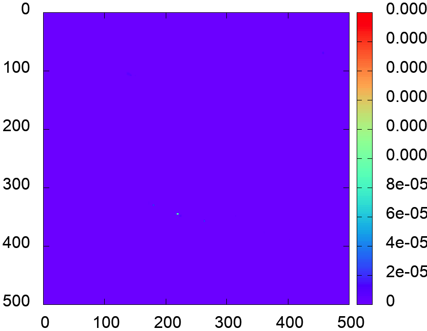
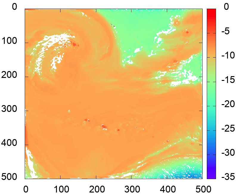
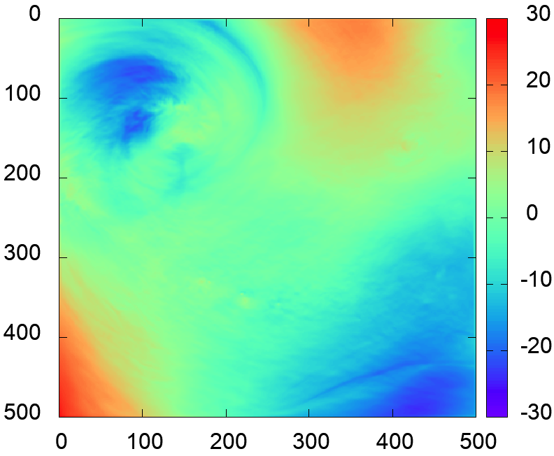
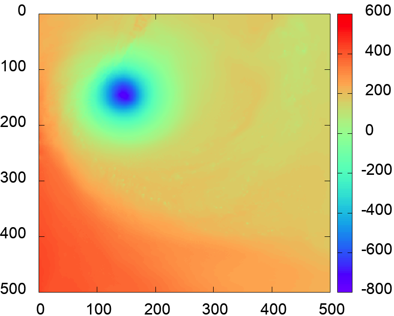
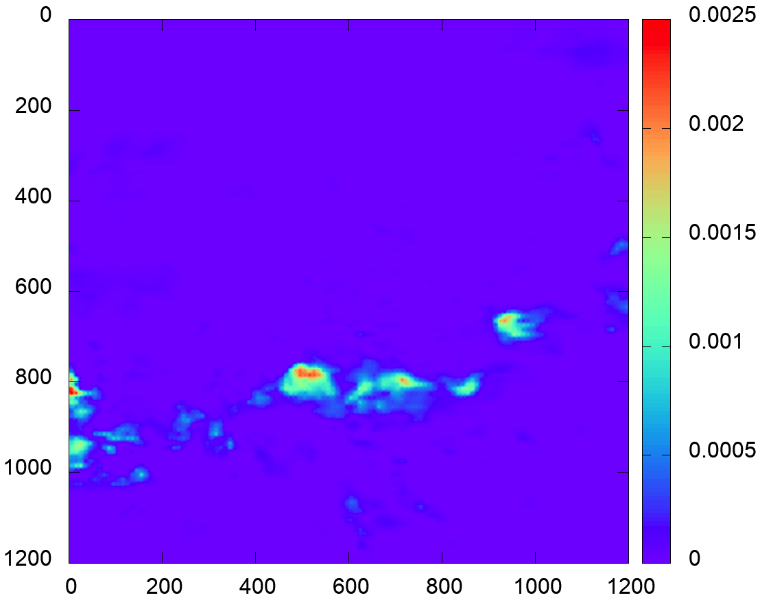
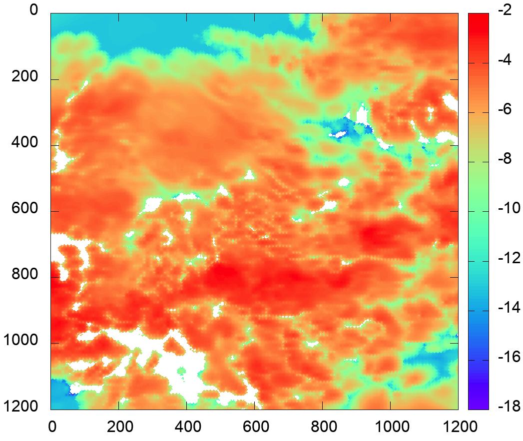
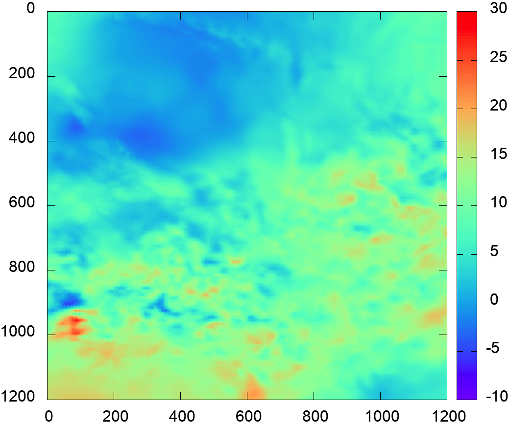
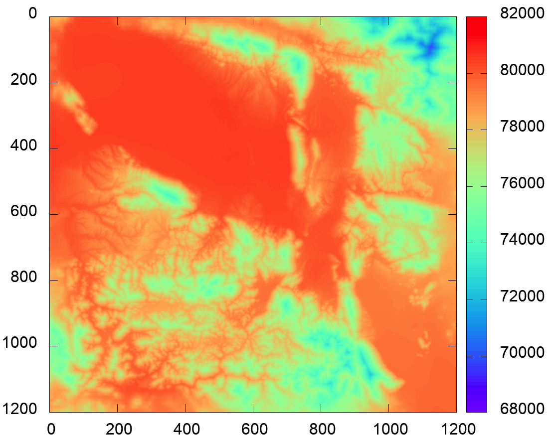
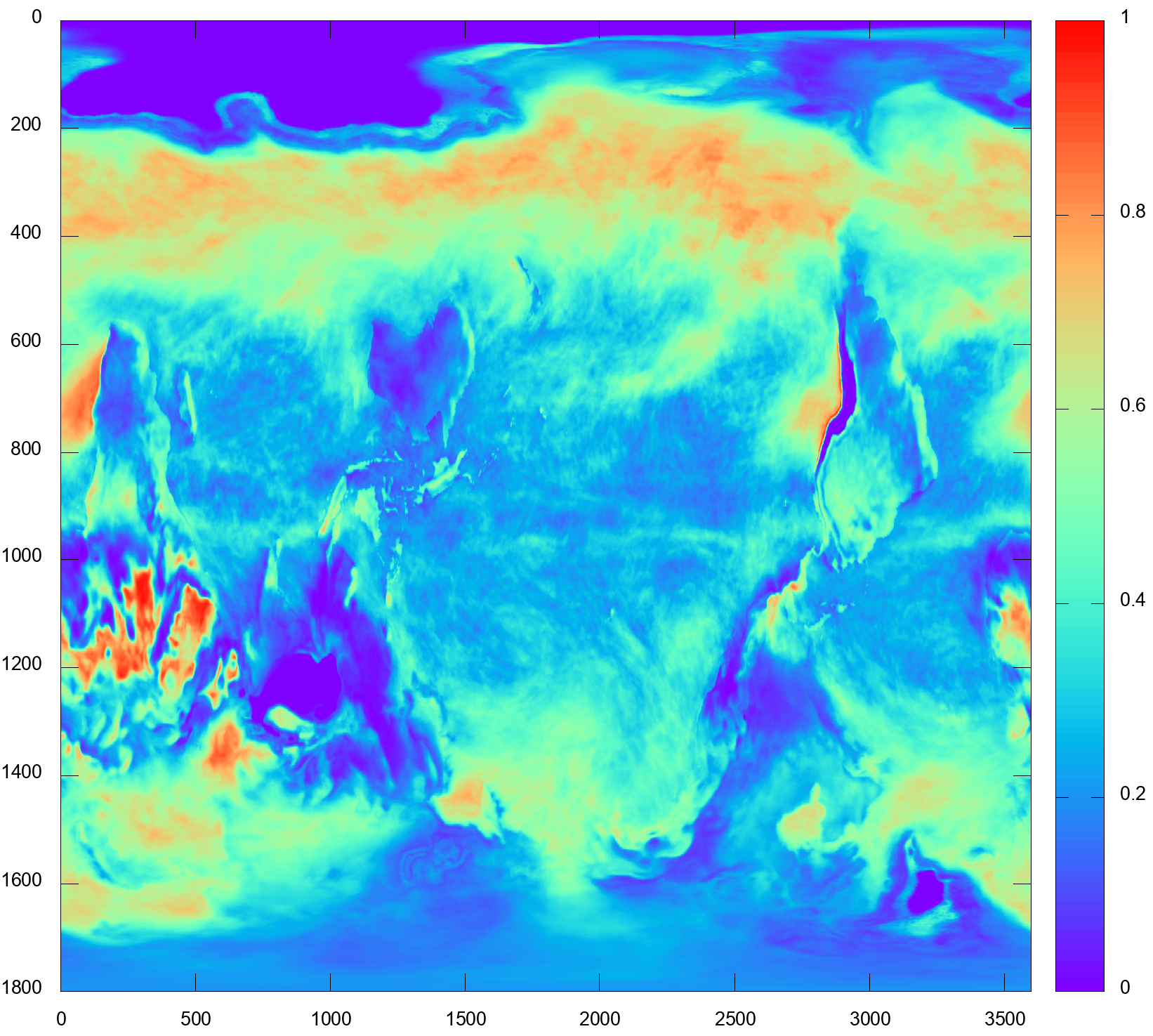
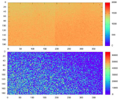
Climate simulation is a typical example that may produce extremely large amounts of data [25, 26]. We include three different climate simulation datasets in our benchmark. The first dataset is from the climate research project at Argonne National Laboratory. It is called CESM-ATM because it was produced based on the climate atmosphere simulation under the Community Earth System Model (CESM). CESM-ATM involves 60+ snapshots(timesteps), each containing 100+ fields with different dimensions. The majority of fields are 2D floating-point arrays (presented in Fig. 1 (a)). Some fields involve the third dimension which represents the number of layers, while each layer is still a 2D array. For those 3D data, it is better to compress them based on 2D format instead of 3D, to be demonstrated later in detail. We provide one snapshot of data (out of 60 snapshots) for CESM-ATM in the SDRBench, because the dataset of 60 snapshots (1.5TB in total) is too large to download for most users and different snapshots of data exhibit similar data features. The fields and total size columns in Table I are for one snapshot of CESM-ATM dataset. The second dataset, Hurricane-ISABEL, is from IEEE Visualization 2004 contest [27]. The dataset simulates the ISABEL hurricane - the strongest hurricane in the 2003 Atlantic hurricane season. The dataset contains 13 floating-point fields in single-precision, and each field is a 3D array with the shape of $100\times 500\times 500$. Fig. 2 demonstrates the visualization of three fields in the Hurricane-ISABEL dataset (generated by Z-checker). The third dataset, named SCALE-LETKF[28], is the simulation data generated by the Local Ensemble Transform Kalman Filter (LETKF) data assimilation package with the Scalable Computing for Advanced Library and Environment - Regional Model (SCALE-RM)[29]. SCALE-LETKF has 13 single-precision floating-point fields each with the shape of $98\times 1200\times 1200$. The visualization results are shown in Fig. 3.

(a) Field: dark_matter_density

(b)   Field: dark_matter_density
                (log-scale)

(c) Field: temperature

(d) Field: velocity_x

Figure 4: Visualization of NYX

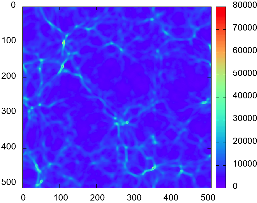
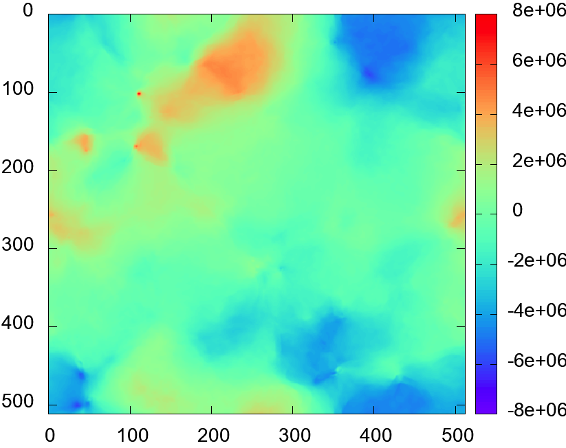
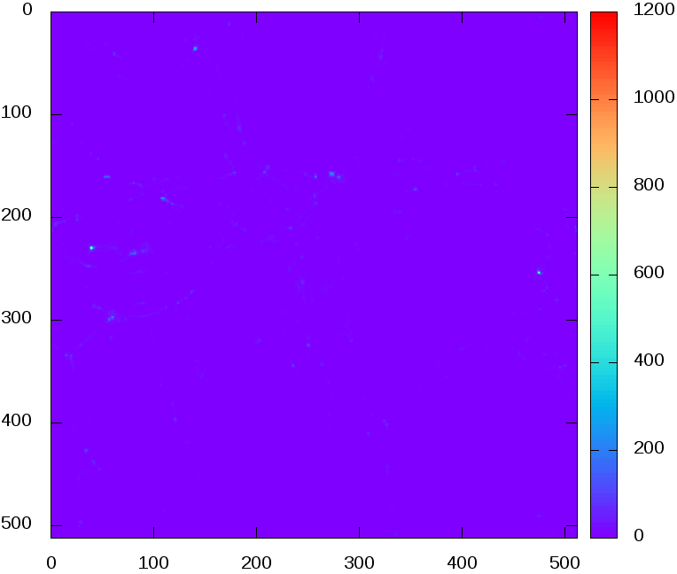
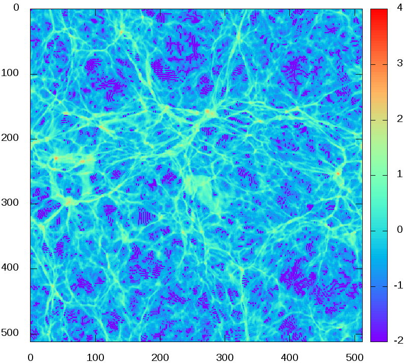
Cosmological N-body simulation investigates extremely large structures such as galaxies and clusters of galaxies composed of numerous moving particles. Our benchmark involves two different cosmological simulation codes - an Hardware/Hybrid Accelerated Cosmology Code (HACC) [3] and an adaptive mesh, compressible cosmological hydrodynamics simulation code (NYX) [30], both of which are widely used in the cosmological research community. The HACC data are composed of 6 1D arrays representing the position and velocity information (denoted by x, y, z, vx, vy, and vz), respectively. The NYX simulation data are post-analysis data composed of 3D arrays in space (such as dark matter density and temperature). Figure 4 shows the visualization results of three fields in NYX dataset.

(a) Field: density

(b) Field: viscocity

(c) Field: velocityy

(d) Field: velocityz

Figure 5: Visualization of Miranda

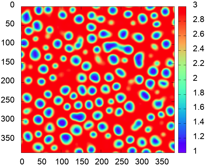
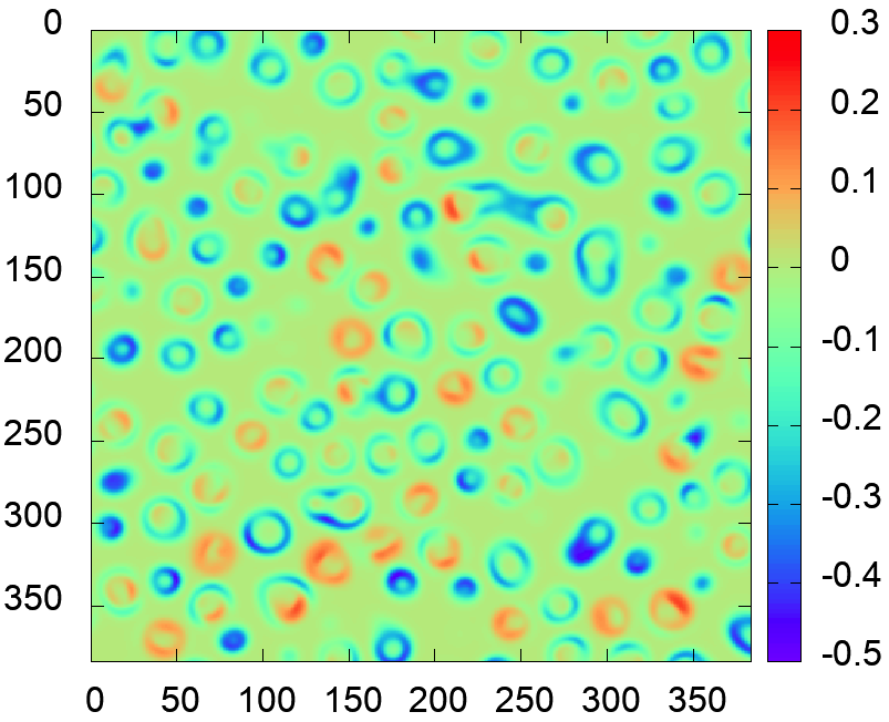
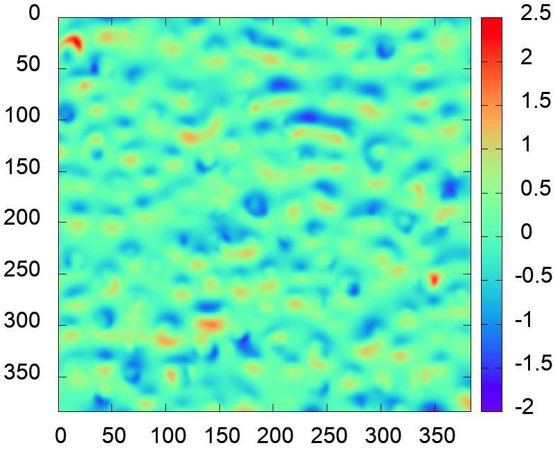
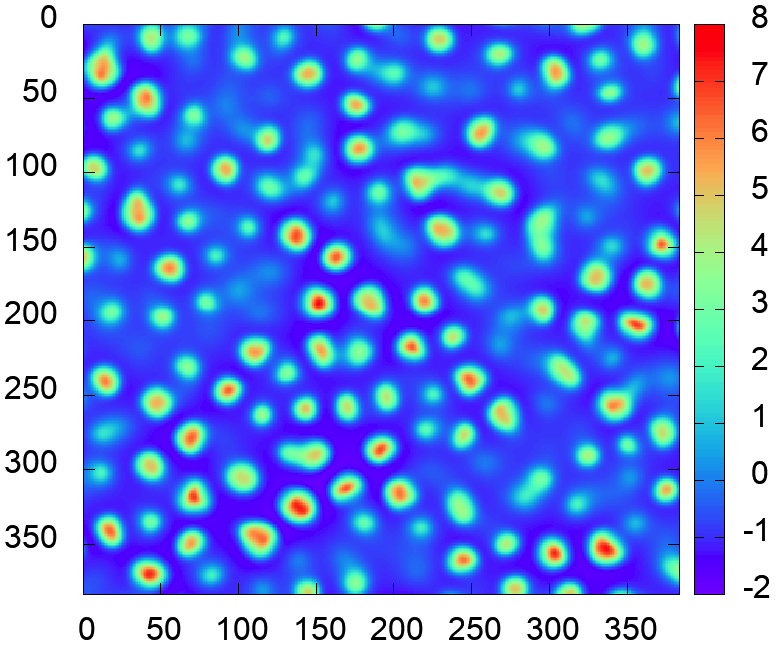
Turbulence simulation aims to solve problems regarding fluid flows by computational fluid dynamics technology. Miranda [31], a radiation hydrodynamics code designed for large-eddy simulation, is included in our dataset. Different from most datasets in our benchmark, the data type of Miranda is 64-bit double-precision floating-point. Miranda has seven fields, and the size of each field is $256\times 384\times 384$. The visualization results are shown in Fig. 5.

QMCPack is an open source ab initio quantum Monte Carlo package for analyzing the electronic structure of atoms, molecules and solids. In the benchmark, we release the dataset (3D, single-precision) for one field called ’einspline’ with two representation formats - raw data and preconditioned data, respectively. The former is the original dataset stored in the memory during the simulation and the latter reorganizes the orders of the elements because this may lead to higher compression ratios according to the data provider.

Molecular dynamics simulation is also included in our benchmark, and one typical example is the Exascale Atomistic Capability for Accuracy, Length, and Time (EXAALT) project [32], which aims to develop a simulation tool to address key fusion and fission energy materials challenges at the atomistic level: extending the burnup of nuclear fuel in fission reactors (dynamics of defects and fission gas clusters in $UO_{2}$), and developing plasma-facing components (tungsten first wall) to resist the harsh conditions of fusion reactors.

Instrument data is also covered by our benchmark, in addition to simulation datasets. Specifically, our benchmark provides the datasets generated/analyzed by EXAFEL project [33]. These data was produced by Linac Coherent Light Source (LCLS) - a free-electron laser facility located at SLAC National Accelerator Laboratory. They are used to analyze biological structures in unprecedented atomic detail for modeling proteins that play a key role in many biological functions. In the benchmark, there are three fields (called ’dark’, ’raw’, and ’calibrated’) provided by the LCLS researcher. Every field has the dimension of $10\times 32\times 185\times 388$, which means 10 3D-images ($32\times 185\times 388$), where ‘32’ is for separate panels in one detector. Fig. 1 (b) visualizes one panel ($185\times 388$) of the ’dark’ field and ’calibrated’ field, respectively.

III-B Characterization of the Scientific Datasets

TABLE II: Properties of NYX Simulation Data

Field	Min	Avg	Max	Range	Entropy	Percentile			Autocorrelation
						1%	99%	range	lag=1	lag=10
velocity_x	-50417k	353.9	31867k	82283k	7.36	-14932k	14032k	28965k	1.000	0.991
velocity_y	-43933k	52.97	56506k	100438k	7.39	-11700k	12729k	24429k	1.000	0.984
velocity_z	-38938k	-65.7	33386k	72324k	7.37	-9340k	7863k	17204k	0.998	0.919
temperature	2281	8453.3	4783k	4780k	7.01	3610	27984	24373	0.916	0.331
dark_matter_density	0	1	13779	13779	7.19	0.000	10.457	10.457	0.775	0.038
baryon_density	0.0580	1	115863	115862	7.1	0.137	7.420	7.283	0.568	0.003

In this section, we characterize the scientific datasets in the benchmark. Due to the space limitation, we just present the results of some fields in NYX, Hurricane-ISABEL, and SCALE-LETKF, and the full reports can be found on the Z-checker website [17].

NYX. Table II presents the data properties of NYX simulation. We can observe that among the six fields, three of them have more than 5000X larger value range than the rest fields. As a result, the value range has to be taken into account if an absolute error bound is used in the compression, otherwise either the compression ratio would be too small or the compression errors would be too large to be available for the post-analysis.

Some datasets such as the dark matter density of NYX should be transformed to log-scale data before performing the visualization analysis, as confirmed by the data providers. Fig. 4 shows one slice image of the dark matter density data based on the original scale and log-scale, respectively. The log-scale data is much easier for the visualization than the original scale, because this dataset spans a very large value range ([0,13779]) while the majority of data are pretty small (the range between 1% percentile and 99% percentile is only 10.45). Accordingly, we adopt the compression based on the log-scale data for such fields (including dark matter density and baryon density), and other fields still apply the original-scale compression.

The autocorrelation analysis indicates that the velocity fields have higher correlation than other fields. The lag 10 autocorrelation of baryon_density is only 0.003 while the lag 10 autocorrelation of velocity_x is 0.991. Therefore, using the same lossy compressor, baryon_density may exhibit a different compression quality compared to velocity_x .

TABLE III: Properties of Hurricane-ISABEL Simulation Data

Field	Min	Avg	Max	Range	Entropy	Percentile			Autocorrelation
						1%	99%	range	lag=1	lag=10
W	-3.241	0.0038	13.3332	16.574	4.489	-0.278	0.456	0.734	0.703	0.148
V	-45.615	3.5531	48.0858	93.7	8.914	-22.666	32.132	54.798	0.998	0.978
U	-53.023	-2.223	39.56	92.581	8.638	-29.244	20.281	49.525	0.996	0.950
P	-3411.741	375.94	3224.4	6636.1	7.747	-738	2018	2756	0.998	0.984
TC	-76.554	-30.793	29.647	106.201	9.682	-72.767	25.076	97.843	1.000	1.000
CLOUD	0	8.6E-06	0.00205	0.002	1.0222	0	0.000253	0.000253	0.809	0.396
PRECIP	0	1.24E-05	0.00751	0.008	0.891	0	0.000314	0.000314	0.864	0.428
QCLOUD	0	6.4E-06	0.00205	0.002	0.484	0	0.000235	0.000235	0.803	0.393
QVAPOR	0	0.0023	0.02	0.02	6.397	0	0.0168	0.0168	0.998	0.984
QGRAUP	0	3.8E-06	0.0073	0.0073	0.38	0	0.000115	0.000115	0.857	0.380

Hurricane-ISABEL. Table III presents the data properties of the 10 fields in Hurricane ISABEL simulation. The value range differs largely on different fields. Specifically, the fields CLOUD, PRECIP, QCLOUD, QGRAUP need to be log-transformed before compression, because the original-scale data cannot be visualized directly (shown in Fig. 2 (a)).

TABLE IV: Properties of Scale-LETKF Simulation Data

Field	Min	Avg	Max	Range	Entropy	Percentile			Autocorrelation
						1%	99%	range	lag=1	lag=10
U	-71.75	5.79	46.67	118.43	7.23	-23.9	18.5	42.4	0.999	0.992
QV	0	0.0043	0.0195	0.0195	7.392	1.21E-06	0.016	0.016	1.000	0.999
QC	0	6.37E-06	0.0030	0.0030	3.924	0	0.000163	0.000163	0.995	0.794
QG	0	1.46E-05	0.0148	0.0148	7.479	0	0.0002	0.0002	0.989	0.822
QI	0	4.17E-06	0.0016	0.0016	4.008	0	7.45E-05	7.45E-05	0.996	0.900
PRES	2285	42841	101820	99534	7.106	2480	99414	96933	1.000	1.000
RH	0	44.64	204.47	204.47	7.115	0.151	97.4	97.2	1.000	0.991
T	181.91	251.06	314.63	132.71	6.621	202	305	104	1.000	1.000
QR	0	1.28E-05	0.00637	0.00637	7.500	0	0.000324	0.000324	0.995	0.887
W	-37.12	-0.0194	26.77	63.89	7.448	-4.94	3.58	8.52	0.997	0.847
QS	0	6.43E-06	0.000756	0.000756	7.494	0	0.000084	0.000084	0.998	0.944
V	-40.15	-0.412	59.42	99.57	7.383	-18.6	23.6	42.2	0.998	0.972

SCALE-LETKF Table IV presents the data properties of SCALE-LETKF simulation. Similar to NYX dataset, some fields including QC, QG, and QR in SCALE-LETKF dataset need to be log-transformed before compression. Fig.3 (a,b) shows one slice image of the QR data based on the original scale and log-scale, respectively, and it confirms that the log-scale is better for visualization than the original scale.

IV The Lossy Compressor Assessment Metrics in SDRBench

In this section, we discuss the metrics to evaluate lossy compressors on scientific datasets.

The compression developers and users generally focus on the following three metrics regarding the distortion of data – maximum absolute error, maximum point-wise relative error, peak-to-signal noise ratio (PSNR). Maximum absolute error is defined as the maximum difference between original data and decompressed data. Maximum point-wise relative error refers to the maximum ratio of the absolute point-wise error to the original data value. PSNR is used to assess the average compression error, and its definition is shown in Formula (1).

$$PSNR=20\cdot\log_{10}{(value\_range)}-10\cdot\log_{10}{(MSE)}.$$ (1)

where value_range and MSE are referred to as the value range of the dataset and mean squared error between the original data and decompressed data.

In addition to the above common metrics, there are some other metrics designed for specific purposes. Autocorrelation of compression errors, for instance, is used to assess the correlation of the compression errors. Distribution of compression errors is also studied to understand the overall distortion of the data in a statistical way. The structural similarity (SSIM) [34] is an index to measure the similarity between the original dataset and decompressed one. The SSIM is the product of three terms (luminance, contrast and structure) evaluating respectively the matching of intensity between the two datasets $a$ and $b$, the variability and the co-variability of the two signals. In statistical terms, luminance, contrast, and structure can be seen as evaluating the bias, variance, and correlation between the two datasets, respectively. SSIM is expressed as

$$SSIM(a,b)=\underbrace{\left(\frac{2\mu_{a}\mu_{b}+c_{1}}{\mu_{a}^{2}+\mu_{b}^{2}+c_{1}}\right)}_{\rm luminance}\underbrace{\left(\frac{2\sigma_{a}\sigma_{b}+c_{2}}{\sigma_{a}^{2}+\sigma_{b}^{2}+c_{2}}\right)}_{\rm contrast}\underbrace{\left(\frac{\sigma_{ab}+c_{3}}{\sigma_{a}\sigma_{b}+c_{3}}\right)}_{\rm structure},$$

with $\mu_{x}$, $\sigma_{x}$ and $\sigma_{xy}$, respectively, being the mean, standard deviation and the cross-covariance of each dataset, and $c_{1}$, $c_{2}$ and $c_{3}$ are constants derived from the datasets. SSIM takes values between $-1$ and $1$, and the closer to $1$, the more similar the two signals are. In Z-checker, we provide two versions of SSIM, one for 1D dataset (directly using the above formula) and the other for 2D dataset (calculating mean SSIM based on every data point in the dataset [35]), respectively.

All the evaluation metrics above are included in our compression assessment tool Z-checker. Z-checker helps lossy compressor developers and users explore the features of scientific datasets and understand the data alteration after compression in a systematic and reliable way. On the one hand, Z-checker combines a group of data analysis components for data compression. On the other hand, Z-checker is implemented as an open-source community tool to which users and developers can contribute and add new analysis components based on their needs. For lossy compressor developers, Z-checker can be used to characterize critical properties (such as entropy, distribution, power spectrum, principal component analysis, and autocorrelation) of any dataset. For lossy compression users, Z-checker can analyze the compression quality (PSNR, normalized MSE, rate-distortion, rate-compression error, spectral, distribution, derivatives) and provide statistical analysis of the compression errors (maximum, minimum, and average error, autocorrelation, distribution of errors). Z-checker can also be extended with more plugins coded in other programming languages/libraries, such as R and FFTW3.

V The Lossy Compressors in SDRBench

Since scientific applications often have strict requirements on the distortion of compression data, our benchmark mainly focuses on the error-controlled lossy compressors. In the following, we describe three state-of-the-art lossy compressors due to the space limitation, and more compressors can be found on the website of our benchmark.

• SZ [25, 26] is an error-bounded compressor, which contains four critical steps: (1) predict the value of each data point; (2) perform linear-scaling quantization; (3) perform customized variable-length encoding; and (4) perform optional lossless compression by compressors such as Zstd [21]. Its particular advantage is allowing users to customize their own data prediction methods based on the data features such that the compression quality could be improved significantly for specific datasets. SZ provides three ways to control the compression errors, including absolute error bound, point-wise relative error bound, and peak-to-signal noise ratio (PSNR). In our assessment, we adopt the latest version which is SZ 2.1.

• ZFP [7] is another error-bounded lossy compressor supporting random access during the decompression because of its block-wise design. It contains five critical steps: (1) align the values in each block to a common exponent; (2) convert the floating-point values to a fixed-point representation; (3) decorrelate values by applying orthogonal transforms; (4) order the transform coefficients; and (5) perform an embedded coding algorithm. ZFP allows users to set an absolute error bound for the compression or specify an integer number (called precision) to obtain a point-wise relative error bounding effect.

• SZ(Hybrid) [36] is a hybrid lossy compressor that integrates a transform-based predictor into the SZ compressor framework. Compared with ZFP which also utilizes the transform-based technology, SZ(Hybrid) has better compression quality on high compression ratio cases because it optimizes the encoding strategy of the transform-based predictor. SZ(Hybrid) adopts a rate-distortion estimation process on the sampling data to select the best predictor between the transform-based predictor and data-fitting-based predictor. The estimation process incurs 50%$\sim$ 100% runtime overhead compared with SZ.

VI Evaluation of Lossy Compressors

In this section, we analyze the three lossy compressors and summarize six takeaways. We focus on critical metrics based on six datasets (NYX, QMCPack, Hurricane-ISABEL, CESM-ATM, EXAFEL, and SCALE-LETKF) due to the space limitation. All compression results were generated by running SZ v2.1, ZFP v0.5.5 and SZ(Hybrid) on Bebop server [37].

(a) REB=1E-2

(b) REB=1E-3

Figure 6: Error Distribution (Hurricane (U))

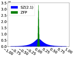
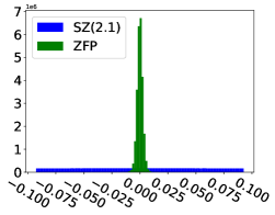
We first verify that the compression errors are within the user defined error bound for all the lossy compressors. Fig. 6 shows the error distribution of field U in Hurricane-ISABEL dataset. The value range of field U is 92.58. The absolute error bounds of U are 0.92 and 0.09 for value-range-based relative error bounds 1E-2 and 1E-3, respectively. The figure confirms that the compression errors are within the absolute error bound. Takeaway 1: Compression Error. The compression errors of SZ have different distributions with different error bound settings. ZFP tends to over preserve the compression precision so that the maximum compression error is much smaller than the error bound.

(a) REB = 1E-2

(b) REB = 1E-4

Figure 7: Compression Speed (NYX)

(a) REB = 1E-2

(b) REB = 1E-4

Figure 8: Decompression Speed (NYX)

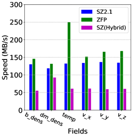
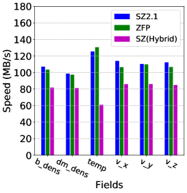
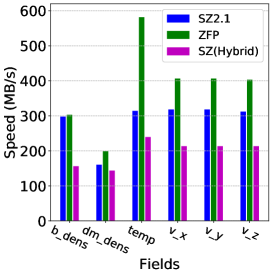
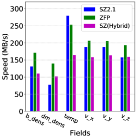
Fig. 7 and Fig. 8 present the compression/decompression speed under the value-range-based relative error bound of 1E-2 and 1E-4, respectively. Takeaway 2: Compression Speed. It is observed that ZFP is about $10\%\sim 100\%$ faster than SZ , and SZ is about $10\%\sim 260\%$ faster than SZ(Hybrid).

(a) CLOUD

(b) PRECIP

(c) V

(d) W

Figure 9: Rate Distortion (Hurricane-ISABEL)

(a) NYX

(b) SCALE-LETKF

(c) QMCPack

(d) Hurricane-ISABEL

Figure 10: Rate Distortion (Four Applications)

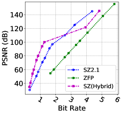
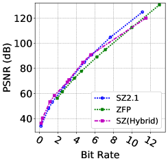
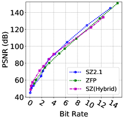
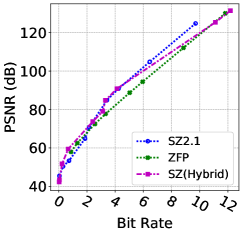
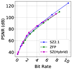
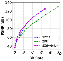
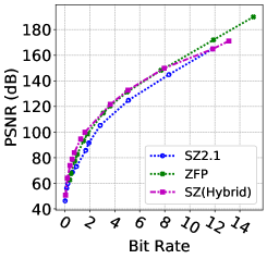
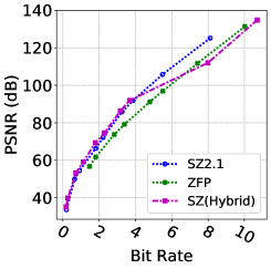
Figure 9 presents the rate-distortion (i.e., bit-rate versus data distortion) of four typical fields in Hurricane-ISABEL simulation, and Fig. 10 presents the rate-distortion for four applications. Bit-rate represents the average number of bits used per data value after the compression, and data distortion is evaluated using PSNR (the higher the better). Takeaway 3: Rate-distortion. When the bit rates are relatively small, SZ(Hybrid) exhibits the best rate-distortion on all four fields of Hurricane-ISABEL and has the best overall rate-distortion on all four applications. On the other hand, SZ is better than SZ(Hybrid) and ZFP when the bit rates are relatively large. For example, on CLOUD field, SZ(Hybrid) has the highest PSNR in the range of [0,2.6], and SZ has the highest PSNR when the bit rate is larger than 2.6.

(a) CESM-ATM(CLOUD)

(b) EXAFEL(calibrated)

Figure 11: Rate Distortion of CESM and EXAFEL

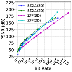
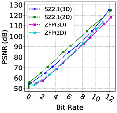
Takeaway 4: Data Dimension. We observe that treating some 3D datasets including CESM-ATM(CLOUD) and EXAFEL(calibrated) as 2D may improve the compression quality, as demonstrated by rate-distortion in Fig. 11. The reason is that CESM-ATM(CLOUD) is composed of 26 2D arrays ($1800\times 3600$ each), and the data is not smooth/consecutive in the third dimension. EXAFEL(calibrated) is composed of 10 3D images ($32\times 185\times 388$ per image), and each 3D image is combined with 32 2D images captured from separate panels. The non smoothness of data in separate panels makes it better to compress the data as 2D. SZ(Hybrid) is not included in Fig. 11 because it does not support compression in 2D mode.

TABLE V: Compression Quality (Compression Ratio, PSNR and SSIM)

Dataset	SZ				ZFP				Compression Ratio of Lossless Compressors
	CR	PSNR	SSIM(1D)	SSIM(2D)	CR	PSNR	SSIM(1D)	SSIM(2D)	ZSTD	C-Blosc2	FPZIP	FPC	ZFP
QMCPack(einspline)	14.35	96	$>$0.9999995	0.9837	14.6	104.2	$>$0.9999995	0.985	1.20	1.01	1.75	1.09	2.21
Hurricane-ISABLE(P)	58.3	68.838	0.999989	0.9963	44.7	64.841	0.997443	0.9877	1.15	1.00	2.11	1.10	1.64
CESM-ATM(CLOUD)	30.75	66.8	0.999988	0.999999	31.5	53.4	0.999734	0.9815	1.66	1.40	2.32	1.54	1.58
EXAFEL (calibrated)	23.4	67.5	0.999999	0.999999	4.73	64.77	0.999999	0.99998	1.96	1.11	1.11	1.00	3.29

Table V presents the PSNR and SSIM (in terms of both 1D and 2D) for the four datasets with different compressors, by tuning the compression ratios to the similar level (except for EXAFEL because the compression ratios of ZFP are always lower than 8:1). Takeaway 5: SSIM and PSNR. It is observed that 1D SSIM is always very close to 1 for any compressor, while 2D SSIM and PSNR can show the discrepancies of compression results more clearly on different compressors. The reason 1D SSIM always approaches to 1 is that the mean, standard deviation and covariance are always very similar between the original data and decompressed data. Some recent studies [35, 38] on visualization shows that 2D SSIM could be more accurate than PSNR in some cases, so we suggest to use both PSNR and 2D SSIM in the evaluation of lossy compression quality.

Table V also contains compression ratios of five state-of-the-art lossless compressors. We include ZFP since it has a lossless mode besides the lossy mode. Takeaway 6: Lossless versus Lossy. Lossless compressors generally have very low compression ratios on scientific datasets. Their compression ratios are in the range of 1$\sim$3 which is far from desired levels to solve the storage and I/O bottleneck problem. Lossy compressors, on the other hand, can reach 20$\times$ higher compression ratio than lossless compressors do, with acceptable data fidelity for post-analysis based on user-specified error bounds. As a result, lossy compressors are more suitable for scientific data compression scenarios.

VII Conclusion and Future Work

In this paper, we release SDRBench, a scientific data reduction benchmark to help compression users and developers assess lossy compressors fairly and conveniently. SDRBench contains scientific datasets, lossy compressor assessment metrics, and state-of-the-art lossy compressors. The 10+ scientific datasets in SDRBench are from different domains including climate simulation, cosmological n-body simulation, turbulence simulation, and others. We also present the evaluation results using SDRBench and summarize six valuable takeaways to help developers and users to have a better understanding of lossy compressors.

• Takeaway 1: Compression Error. Lossy compressors have different compression error distributions. In addition, ZFP tends to over preserve the compression precision.

• Takeaway 2: Compression Speed. Lossy compressors have varied compression speed. For example, ZFP is about $10\%\sim 100\%$ faster than SZ.

• Takeaway 3: Rate-distortion. Currently, no lossy compressor can always outperform the others in terms of rate-distortion.

• Takeaway 4: Data Dimension. For some 3D data such as the CLOUD field of CESM-ATM, treating them as 2D data may improve the compression quality.

• Takeaway 5: SSIM and PSNR. 2D SSIM is better than 1D to show the discrepancies of compression results. We suggest use 2D SSIM and PSNR in the evaluation of lossy compression quality.

• Takeaway 6: Lossless versus Lossy. Lossless compressors have very low compression ratio (usually 1$\sim$3) on scientific datasets, while lossy compressors can achieve $20\times$ higher compression ratio on the same dataset than lossless compressors.

In the future, we will include more datasets in different scientific domains and more lossy compressors in the benchmark.

VIII Acknowledgments

This research was supported by the Exascale Computing Project (ECP), Project Number: 17-SC-20-SC, a collaborative effort of two DOE organizations – the Office of Science and the National Nuclear Security Administration, responsible for the planning and preparation of a capable exascale ecosystem, including software, applications, hardware, advanced system engineering and early testbed platforms, to support the nation’s exascale computing imperative. The material was supported by the U.S. Department of Energy, Office of Science, under contract DE-AC02-06CH11357, and supported by the National Science Foundation under Grant No. 1619253. We acknowledge the computing resources provided on Bebop, which is operated by the Laboratory Computing Resource Center at Argonne National Laboratory.

References

- [1] X. Liang, S. Di, D. Tao, S. Li, B. Nicolae, Z. Chen, and F. Cappello, “Improving performance of data dumping with lossy compression for scientific simulation,” in 2019 IEEE International Conference on Cluster Computing (CLUSTER), 2019, pp. 1–11.
- [2] A. M. Gok, S. Di, A. Yuri, D. Tao, V. Mironov, X. Liang, and F. Cappello, “PaSTRI: A novel data compression algorithm for two-electron integrals in quantum chemistry,” in IEEE International Conference on Cluster Computing (CLUSTER). IEEE, 2018, pp. 1–11.
- [3] S. Habib, V. Morozov, N. Frontiere, H. Finkel, A. Pope, K. Heitmann, K. Kumaran, V. Vishwanath, T. Peterka, J. Insley et al., “Hacc: extreme scaling and performance across diverse architectures,” Communications of the ACM, vol. 60, no. 1, pp. 97–104, 2016.
- [4] D. Tao, S. Di, Z. Chen, and F. Cappello, “Exploration of pattern-matching techniques for lossy compression on cosmology simulation data sets,” in High Performance Computing. Springer International Publishing, 2017, pp. 43–54.
- [5] D. Tao, S. Di, Z. Chen, and F. Cappello, “In-depth exploration of single-snapshot lossy compression techniques for N-body simulations,” in 2017 IEEE International Conference on Big Data (Big Data). IEEE, 2017, pp. 486–493.
- [6] S. Li, S. Di, K. Zhao, X. Liang, Z. Chen, and F. Cappello, “SDC resilient error-bounded lossy compressor,” https://arxiv.org/abs/2010.03144, 2020, online.
- [7] P. Lindstrom, “Fixed-rate compressed floating-point arrays,” IEEE transactions on visualization and computer graphics, vol. 20, no. 12, pp. 2674–2683, 2014.
- [8] J. Tian et al., “Cusz: An efficient gpu-based error-bounded lossy compression framework for scientific data,” in Proceedings of the ACM International Conference on Parallel Architectures and Compilation Techniques, ser. PACT ’20. ACM, 2020, p. 3–15.
- [9] S. Jin, S. Di, X. Liang, J. Tian, D. Tao, and F. Cappello, “DeepSZ: A novel framework to compress deep neural networks by using error-bounded lossy compression,” in Proceedings of the 28th International Symposium on High-Performance Parallel and Distributed Computing, ser. HPDC ’19. ACM, 2019, pp. 159–170.
- [10] J. Tian, S. Di, C. Zhang, X. Liang, S. Jin, D. Cheng, D. Tao, and F. Cappello, “Wavesz: A hardware-algorithm co-design of efficient lossy compression for scientific data,” in Proceedings of the 25th ACM SIGPLAN Symposium on Principles and Practice of Parallel Programming, ser. PPoPP ’20. ACM, 2020, p. 74–88.
- [11] S. Li, S. Di, K. Zhao, X. Liang, Z. Chen, and F. Cappello, “Towards end-to-end SDC detection for HPC applications equipped with lossy compression,” in 2020 IEEE International Conference on Cluster Computing, 2020, pp. 326–336.
- [12] D. Tao, S. Di, X. Liang, Z. Chen, and F. Cappello, “Optimizing lossy compression rate-distortion from automatic online selection between SZ and ZFP,” IEEE Transactions on Parallel and Distributed Systems, vol. 30, no. 8, pp. 1857–1871, 2019.
- [13] S. Li, S. Di, X. Liang, Z. Chen, and F. Cappello, “Optimizing lossy compression with adjacent snapshots for n-body simulation data,” in 2018 IEEE International Conference on Big Data (Big Data), 2018, pp. 428–437.
- [14] X. Liang, S. Di, D. Tao, S. Li, S. Li, H. Guo, Z. Chen, and F. Cappello, “Error-controlled lossy compression optimized for high compression ratios of scientific datasets,” 2018 IEEE International Conference on Big Data (Big Data), pp. 438–447, 2018.
- [15] K. Zhao, S. Di, X. Liang, S. Li, D. Tao, Z. Chen, and F. Cappello, “Significantly improving lossy compression for HPC datasets with second-order prediction and parameter optimization,” in Proceedings of the 29th International Symposium on High-Performance Parallel and Distributed Computing, ser. HPDC ’20. ACM, 2020, pp. 89–100.
- [16] X. Liang et al., “Optimizing multi-grid based reduction for efficient scientific data management,” https://arxiv.org/abs/2010.05872, 2020, online.
- [17] D. Tao, S. Di, H. Guo, Z. Chen, and F. Cappello, “Z-checker: A framework for assessing lossy compression of scientific data,” The International Journal of High Performance Computing Applications, vol. 33, no. 2, pp. 285–303, 2019.
- [18] Squash Compression Benchmark, https://quixdb.github.io/squash-benchmark/, online.
- [19] TurboBench, https://github.com/powturbo/TurboBench, online.
- [20] L. P. Deutsch, “Gzip file format specification version 4.3,” 1996.
- [21] Zstd, https://github.com/facebook/zstd/releases, online.
- [22] Large Text Compression Benchmark, http://mattmahoney.net/dc/text.html, online.
- [23] Silesia compression corpus, http://sun.aei.polsl.pl/ sdeor/index.php?page =silesia, online.
- [24] The Canterbury Corpus, https://corpus.canterbury.ac.nz/descriptions/, online.
- [25] D. Tao, S. Di, Z. Chen, and F. Cappello, “Significantly improving lossy compression for scientific data sets based on multidimensional prediction and error-controlled quantization,” in 2017 IEEE International Parallel and Distributed Processing Symposium. IEEE, 2017, pp. 1129–1139.
- [26] S. Di and F. Cappello, “Fast error-bounded lossy hpc data compression with sz,” in 2016 IEEE International Parallel and Distributed Processing Symposium. IEEE, 2016, pp. 730–739.
- [27] Hurricane ISABEL dataset, http://sciviscontest-staging.ieeevis.org/2004/data.html, online.
- [28] G.-Y. Lien, T. Miyoshi, S. Nishizawa, R. Yoshida, H. Yashiro, S. Adachi, T. Yamaura, and H. Tomita, “The near-real-time scale-letkf system: A case of the september 2015 kanto-tohoku heavy rainfall,” SOLA, vol. 13, pp. 1–6, 01 2017.
- [29] Scalable Computing for Advanced Library and Environment Regional Model, https://scale.riken.jp/scale-rm/, online.
- [30] NYX simulation, https://amrex-astro.github.io/Nyx, online.
- [31] Miranda simulation, https://wci.llnl.gov/simulation/computer-codes/miranda, online.
- [32] EXAALT project, https://www.exascaleproject.org/project/exaalt-molecular-dynamics-at-the-exascale-materials-science/, online.
- [33] EXAFEL project, https://www.exascaleproject.org/project/exafel-data-analytics-exascale-free-electron-lasers/, online.
- [34] Z. Wang, A. C. Bovik, H. R. Sheikh, and E. P. Simoncelli, “Image quality assessment: from error visibility to structural similarity,” IEEE transactions on image processing, vol. 13, no. 4, pp. 600–612, 2004.
- [35] Z. Wang and A. C. Bovik, “Mean squared error: Love it or leave it? a new look at signal fidelity measures,” IEEE Signal Processing Magazine, vol. 26, no. 1, pp. 98–117, Jan 2009.
- [36] X. Liang, S. Di, S. Li, D. Tao, B. Nicolae, Z. Chen, and F. Cappello, “Significantly improving lossy compression quality based on an optimized hybrid prediction model,” in Proceedings of the International Conference for High Performance Computing, Networking, Storage and Analysis, 2019, pp. 1–26.
- [37] LCRC Bebop cluster, https://www.lcrc.anl.gov/systems/resources/bebop.
- [38] A. Baker, D. Hammerling, and T. Turton, “Evaluating image quality measures to assess the impact of lossy data compression applied to climate simulation data,” in Computer Graphics Forum, vol. 38, 06 2019.