Pretty good quantum state transfer on isotropic and anisotropic Heisenberg spin chains with tailored site dependent exchange couplings

Abstract

Using a global optimization algorithm we obtain spin chains with site-dependent exchange coefficients which allow almost perfect quantum state transfer between the extremes of the chains without any further time-dependent external control. We consider chains with isotropic and anisotropic Heisenberg Hamiltonian with up to 100 spins. The method allow us to choose the arrival of the transferred state by changing the range available to the exchange coupling strengths. We consider short transferred times, in particular shorter than those achievable with known time-dependent control schemes. The chains obtained with the optimization method show some remarkable and interesting traits as, for instance, the scaling of the magnitude of the exchange couplings needed to achieve near perfect state transfer with the length of the chain and the arrival time. This scaling makes it possible to decide if the chain with site-dependent coefficients can be implemented in an actual system according to the range of interactions allowed in it. We compare the robustness of the transmission protocol against static disorder on the exchange coefficients using different figures of merit, which allow us to conclude that the isotropic Heisenberg chain is the best option when compared with anisotropic chains. This comparison is relevant since the method allow us to start with chains that all achieve near perfect quantum state transfer, regime that was not available previously in these chains without time-dependent external control.

1 Introduction

The transfer of quantum state along communication channels has been under study for almost two decades now as a task of primordial importance to Quantum Information Processing [1]. The cornerstone of the subject on quantum spin chains was laid by Bose [2, 3], who introduced the figure of merit to analyze the quality of the resulting transfer processes.

The most simple transfer protocol on a spin chain can be described rather easily: a given state is prepared at one extreme of the chain and after some time another state, the transferred one, is retrieved at the other extreme. The transfer is better for larger values of the fidelity, and perfect if the state retrieved is the same that the one that was prepared, which corresponds to the maximum value allowed to the fidelity.

The dynamical behaviour between the preparation and retrieval times can be controlled but, in many cases, it is preferred that the time evolution of the quantum state is governed only by the time-independent spin chain Hamiltonian, which depends only on the exchange couplings between the spins on the chain. The unforced dynamics is preferred under the rationale that the precise tuning of the control fields applied to the quantum spin chain add other sources of noise that spoil the state transfer process [4, 5, 6, 7, 8]. However, the strength of the exchange couplings can be modulated to improve the quality of the transfer process, resulting in a number of strategies and dynamical regimes [4, 5, 6, 7, 8, 9, 10, 11, 12, 13]

The addition of noise sources is problematic enough but it is not the only drawback in actual implementations, since the strength of the coupling between the spin chain and the control fields and the frequency spectrum available are also causes for concern [14].

Despite what has been said above, much progress has been made in the field of controlled state transfer, from the study of the most basic aspects of controllability [15, 16, 18, 17], to obtaining particular states in different types of chains [23, 19, 21, 22]. There is a host of physical systems where some quantum state transfer process can be implemented [24, 25, 26, 27, 28, 29, 30, 31]. The strategies to control a given chain are also multiple, varying from using only one actuator [18, 19, 20], two actuators [33] or even controlling almost all (or all) the spins on the chain [34, 35, 36].

On the other hand, perfect state transfer without other interactions than the exchange couplings between the spins of the chain can only be achieved in chains with the so called XX Hamiltonian [5]. The Heisenberg Hamiltonian only admits what has been termed pretty good [38, 37, 39, 40] or near perfect state transfer, i.e. choosing adequate values for the exchange couplings strength it is possible to obtain fidelity values differentially close to unity. This scenario can be rigorously proved for chains whose length is of the form $N=2^{k}$, where $k$ is some natural number. It is interesting that these results can be proved using linear algebra theorems that provide insights about the Hamiltonian spectrum.

Regrettably, the theorems that assure that the pretty good state transfer regime exists do not provide neither the order of magnitude of the couplings nor the transmission time at which to look for them. Taking this into account, the optimization of the fidelity as a function of the exchange couplings strength and the transfer time can offer a different approach to the problem. There has been attempts in this direction, for instance in Ref. [41] machine learning is employed to obtain the exchange couplings of the XX Hamiltonian that is associated to perfect state transfer. We are interested in calculate a set of parameters of the Hamiltonian that places us in the pretty good transfer regime. That is, we do not require the best set, but a very good set of parameters. The problem will be written as the finding of a set of parameters that produce a (very good local) maximum in a cost function.

These class of problems, where we look for good maximum of an arbitrary cost function, are suitable to be treated by stochastic optimization methods. In particular, in this paper we use a method developed by one of us, which has been shown to be very efficient in optimizing functions in parameter space of dimensions even greater than those of interest in this study: the pivot method (PM) for global optimization [42, 43]. The pivot method is a stochastic method to search for the global minimum of a multiple-minimum function defined on a high-dimensional phase space. To find the global minimum of a high-dimensional corrugated landscape is, in general, a NP-hard problem, and therefore there is not a stochastic method that can assure that the global minimum is reached. However, the pivot method has shown to be an efficient method to find a very good minimum, that actually is what we need in the search for good quantum state transfer in chain-spin systems described in this paper.

The paper is organized as follows, In Section 2 the model Hamiltonians to be considered are introduced together with the transfer protocol and the figures of merit that quantify the quality of the transfer process, in particular the relationship between the fidelity of transmission and the transferred population, which is the probability that a single excitation is transferred from one end of the chain to the other. In this Section we also describe how the optimization algorithm must be implemented to find the site-dependent exchange couplings that maximize the transferred population for a chosen transferral time, at the same time we introduced all the notation related to the numerical procedure.

In Section 3 the transfer properties of isotropic Heisenberg spin chains with modulated exchange coupling coefficients are thoroughly analyzed. Particular emphasis is placed on obtaining chains that transmit states with high fidelity for different transfer (or arrival) times. It is shown that the magnitude of the largest exchange coefficient of a modulated chain depends on the arrival time and an approximate formula that fits the dependency is proposed. It is studied how the transmission of a chain whose exchange coefficients have been optimized is affected by the presence of static disorder. It is shown that the transferred population shows scaling properties as a function of time when comparing the transfer of chains, of fixed length, but whose coefficients have been optimized for different arrival times. We also present a brief discussion about the quality of the transfer protocol if the initial state can not be prepared exactly like the protocol prescribes. Once the relationship between the chain length and the maximum value of the exchange coefficients needed to achieve near perfect quantum state transfer at a given arrival time is established, we discuss in which kind of physical system it could be possible to implement chains like the ones treated in the Section.

The analysis described in the paragraph above is repeated in Section 4 for anisotropic Heisenberg spin chains. The conclusions and the discussion of our results are presented in Section 5 where we discuss the different dynamical behaviours that appear in the disordered spin chains.

2 Model Hamiltonians, transfer protocol and Methods

The XXZ Hamiltonian of a quantum spin chain with only nearest-neighbor interactions can be written as

$$H=-\sum_{i=1}^{N-1}J_{i}\left(\sigma_{i}^{x}\sigma_{i+1}^{x}+\sigma_{i}^{y}\sigma_{i+1}^{y}+\Delta\sigma_{i}^{z}\sigma_{i+1}^{z}\right),$$ (1)

where $N$ is the number of spins, or the length of the chain, the $\sigma$’s are the Pauli matrices, the $J_{i}$’s are the exchange coupling strengths, $J_{i}>0,\forall i$, and $\Delta$ is an anisotropy parameter. The Heisenberg Hamiltonian correspond to the isotropic case, $\Delta=1$ and $\Delta=0$ is known as the XX Hamiltonian. Note that the Hamiltonian in Eq. (1) is adimensional, besides we take $\hbar=1$.

The Hamiltonian in Eq. (1) commutes with the total magnetization in the $z-$direction

$$\left[H,\sum_{i}\sigma_{i}^{z}\right]=0,$$ (2)

so the Hamiltonian can be diagonalized in subspaces with fixed number of excitations, i.e. in subspaces with a given number of spins up. It is customary to use the computational basis, where for a single spin $|0\rangle=|\downarrow\rangle$ and $|1\rangle=|\uparrow\rangle$, so $|\mathbf{0}\rangle=|0000\ldots 0\rangle$ is the state with zero spins up of the whole chain, and

$$\sum_{i=1}^{N}\sigma_{i}^{z}|\mathbf{0}\rangle=-N|\mathbf{0}\rangle.$$ (3)

The $N$ states with a single spin up are denoted as follows

$$|\mathbf{1}\rangle=|10\ldots 0\rangle,|\mathbf{2}\rangle=|010\ldots 0\rangle,\ldots,|\mathbf{N}\rangle=|00\ldots 1\rangle.$$ (4)

i.e. the state $|\mathbf{j}\rangle$ is the state of the chain with only the $j$-th spin up. The one-excitation basis plays a fundamental role in the simplest transfer protocol. In this protocol the initial state of the chain, $|\Psi(0)\rangle$, is prepared as

$$|\Psi(0)\rangle=|\psi(0)\rangle\otimes|\mathbf{0}\rangle_{N-1}$$ (5)

where $|\psi(0)\rangle=\alpha|0\rangle+\beta|1\rangle$, is an arbitrary one-spin pure state, with $\alpha$ and $\beta$ complex constants such that $|\alpha|^{2}+|\beta|^{2}=1$, and $|\mathbf{0}\rangle_{N-1}$ is the state without excitations of a chain with $N-1$ spins. The state in Eq. (5) can be rewritten as

$$|\Psi(0)\rangle=\alpha|\mathbf{0}\rangle+\beta|\mathbf{1}\rangle.$$ (6)

Using the time evolution operator

$$U(t)=\exp{(-iHt)},$$ (7)

the state of the chain at time $t$ can be obtained as

$$|\Psi(t)\rangle=U(t)|\Psi(0)\rangle=\alpha U(t)|\mathbf{0}\rangle+\beta U(t)|\mathbf{1}\rangle.$$ (8)

It is clear that the state transfer is perfect when for some time $T_{per}$ the state of the chain is given by

$$|\Psi(T_{per})\rangle=e^{i\theta}\left(\alpha|\mathbf{0}\rangle+\beta|\mathbf{N}\rangle\right),$$ (9)

where $\theta$ is some real arbitrary phase. So, the transfer fidelity as a function of time is calculated as

$$f_{\alpha,\beta}(t)=|\alpha\langle\Psi(t)|\mathbf{0}\rangle+\beta\langle\Psi(t)|\mathbf{N}\rangle|^{2}.$$ (10)

The fidelity in Eq. (10) depends on the particular initial state, Eq. (6), chosen to be transferred. Usually, to quantify the quality of the state transfer protocol, it is introduced the average of $f_{\alpha,\beta}(t)$ over all the possible values of $\alpha$ and $\beta$. It can be shown that this averaged fidelity, $F(t)$, can be written as

$$F(t)=\frac{\sqrt{|P(t)|}}{3}+\frac{P(t)}{6}+\frac{1}{2},$$ (11)

where

$$P(t)=|\langle\mathbf{1}|U(t)|\mathbf{N}\rangle|^{2}$$ (12)

is called the transferred population between the first and last sites of the chain, and we assume that $\cos(\gamma)=1$, where $\gamma=arg(f_{\alpha,\beta}(t))$, as in Ref. [2]. The pretty good transfer occurs when

$$P(t)=1-\epsilon,$$ (13)

where $\epsilon\ll 1$.

The optimization algorithm

The XX Hamiltonian shows perfect state transfer for a number of Exchange Couplings Distributions (ECDs). For ECD we understand a particular set of values $\{J_{i}\}_{i=1}^{N-1}$ that univocally determines a particular Hamiltonian for a chain. For example, it is well known that the ECD given by $J_{i}=\sqrt{i(N-i)}$ determines the XX Hamiltonian that shows perfect state transfer at time $T_{per}=\pi/2$.

For Heisenberg chains $T_{per}$ it is not known, so the optimization method can be designed to obtain an ECD for a chosen transfer time.

Our method allow us to choose the transfer time $T$, however we will focus on the range $T\in\left[\frac{N}{2},5N\right]$. The range chosen allows us to compare our results for the Heisenberg Hamiltonian with those that are well known for the XX Hamiltonian. There is not an obvious upper value for the transfer times to be explored other than the search of fast transfer times. It is worth to mention that transfer times on the order $10N$ are achievable controlling the dynamics by applying external magnetic fields to the spins at the extremes of an unmodulated chain (with all its couplings equal), so obtaining smaller transfer times for uncontrolled state transfer could make preferable the task of engineering the couplings strength rather than implementing the control fields [1].

Since the global optimization procedure always find a good maximum for the function that is being optimized, in our case the transferred population $P(T)$, where $T$ is the arrival (or transfer) time, we proceed to look for the maximum transferred population inside a hypercube $0\leq J_{i}\leq J_{max}$ containing the possible values for the exchange couplings. The hypercube is the high-dimensional phase space (a N-dimensional hypercube of size $J_{max}$) that was mentioned in the Introduction. In the context of optimization methods the function that is maximized or minimized is usually called cost function.

Figure 1: The cartoon depicts the ingredients of the procedure designed to find EC distributions that can be used to achieve near perfect QST. a) A centro-symmetric spin chain with five spins and only two different exchange couplings $J_{1}$ and $J_{2}$. b) For the five spin chain a ECD that optimize the cost function for an arrival time $T$ is obtained using the pivot method . The ECD is denoted by $\{J^{(k)}\}_{T}=(J^{(k)}_{1},J^{(k)}_{2})$, which is a point in the hypercube with side length $J_{max}^{(k)}$. c) The smaller hypercube with side length $J_{max}^{(1)}$ and the second one smaller, with side length $J_{max}^{(2)}=J_{max}^{(1)}+\delta$, are depicted using light blue and blue squares. The corresponding ECD that optimize the cost function for each hypercube is depicted as a starry dot inside the hypercube.

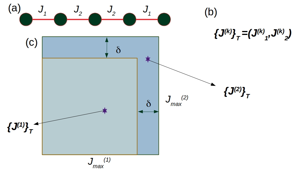
There is not a known relationship between the maximum value necessary for the couplings $J_{i}$ to achieve near perfect quantum state transfer at a given time $T$, for this reason it is useful to consider a succession of values $J^{(k)}_{max}$. For each one of this values of the hypercube side length the pivot method determines an ECD denoted as $\{J_{k}\}_{T}$ where $T$ is the transfer time. The succession of lengths of the hypercube side is given by $J_{max}^{(k)}=J_{max}^{(1)}+(k-1)\delta J$, for $k=1,2,3,\ldots$ and $\delta J=0.5$. As the rigorous results about the existence of the pretty good transfer scenario are proved for centro-symmetric ECDs, we impose this restriction to the exchange couplings, $J_{N-i}=J_{i}\;;\;i=1,\cdots,[N/2]$. The cartoon in Fig. 1 depicts the main ingredients of the procedure to find the exchange coupling distributions that will lead to a chain that can attain the near perfect QST. On the other hand, it is clear that the optimization of the transferred population in a particular hypercube with side length $J_{max}^{(k)}$ provides a optimized value for the transferred population,that we denote as $P^{(k)}$, and that depends on the side length.

Figure 2: The exchange coupling distribution $\{J^{(k)}\}_{T}$ vs the length of the hypercube side $J_{max}$ for a system of $N=30$ spins. As explained in the text, the ECDs corresponding to a system with $N=30$ have $15$ different exchange couplings, which are shown in the figure using colored lines and symbols. The ECDs were obtained using the pivot method for arrival time $T=2N$ . Each set of points of a given colour corresponds to a the values of a given exchange coupling, for instance the black dots correspond to $J_{1}$, the red ones to $J_{2}$ and so on. The figure clearly shows that the particular values of each exchange coupling strength $J_{i}$ depend on $J_{max}$. The black dashed line correspond to $J=J_{max}$ and is used a guide to the eye. Note that for small values of $J_{max}$ the exchange couplings strengths are all close to $J_{max}$, while for large values of $J_{max}$ the pivot method does not find values of $J_{j}$ that further optimize the population transfer and each exchange coupling $J_{i}$ reaches a plateau.

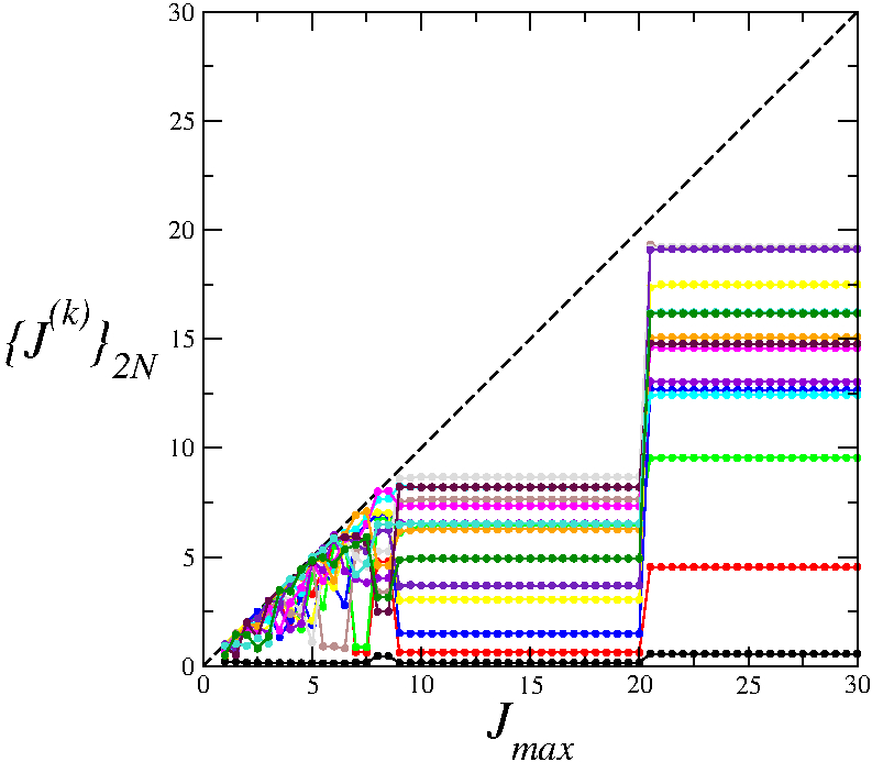
Before proceeding with the analysis of the results that can be obtained using the pivot method, we want stress that there is not a simple way to choose the actual value of $\delta J$. From what is known for the Heisenberg and XX models it is a fair assumption that, for models within the $XX$ universality, the pretty good transfer scenario could be reached with exchange couplings bounded by $N/2$, since this is the value that correspond to the maximal exchange coupling for the perfect state transfer case in the XX model. Nevertheless, the perfect state transfer happens for transfer times that are independent of the chain length so it can be also expected that the bound on the exchange couplings are a decreasing function of the transferral time (this is confirmed by the results that are shown latter in the paper). So $\delta J=0.5$ is a compromise between the different scales that we thought could be present when dealing with models with different values of $\Delta$ and arrival times. In this sense, the value chosen is not optimal, but allow us to search for optimal values of the exchange coupling distribution increasing the volume of the hypercube and starting the search from a “good” initial ECD.

The workings of the pivot method are as follows. Starting from an initial set of points in the phase space on which the cost function depends, the method explores this space until an optimal value is found [42, 43]. In our case each point is an ECD that determines a Hamiltonian. Using the spectrum and eigenvalues of the Hamiltonian the transferred population $P(t)$ is determined for a transfer time $T$ using Eq. (12). The pivot method finds the largest possible value of the transferred population, $P^{(k)}(T)$, inside an hypercube of side $J^{(k)}_{max}$.

Fig. 2 shows the typical results that can be found from a run of the procedure described in the paragraphs above. The Hamiltonian considered is the isotropic one. The figure shows the values of the fifteen different EC values in $\{J^{(k)}\}_{T}$, for a chain with $N=30$ spins as functions of the length of the hypercube side and for a transfer time $T=2N$. The value of a particular coupling changes in a random-walk way when the length of the hypercube size is increased, eventually reaching a large plateau.

The data shown in Fig. 2 was obtained starting from a ECD with $J_{i}^{(1)}=1,\forall i$. We run the PM algorithm to find the largest possible value for the transferred population $P^{(2)}$ corresponding to an ECD such that $J_{i}^{(2)}\leq J_{max}^{(2)}$. Then, the length of the hypercube side was increased to $J_{max}=J_{max}^{(3)}$ and the PM was run again. The algorithm was employed up to $J_{max}^{(K)}=N$ for some $K$. As usual for stochastic global optimization algorithms, we apply to the output set a deterministic gradient algorithm [44] in order to obtain a better accuracy. Throughout this work, mainly in the figures, we will refer to a succession of points $(J_{max}^{(k)},P^{(k)}(T)))$ as the transferred population as a function of $J_{max}$, as if it were effectively a function. This is done for brevity and under the understanding that each point of the succession $P^{(k)}(T)$ must be calculated for an arrival time $T$ and with a specifically designed distribution of coefficients $J_{max}^{(k)}$. In the same sense, once an ECD has been designed to achieve a high TP at a given arrival time $T$ the function in Eq. (12) can be evaluated at any time.

The procedure described in the paragraph above is not the most general but, as we will show latter, results in ECDs with very good properties, in particular the procedure is able to find the regime where $P(t)=1-\epsilon$.

3 Results: Quantum state transfer: the Heisenberg Hamiltonian

Figure 3: The transferred population for a chain with Heisenberg Hamiltonian and $N=30$ spins. The data corresponds to arrival times $T=N/2,N,2N$ and $3N$, which are depicted as black, red, green and blue dots, the lines joining the dots are used as a guide for the eye. Each point corresponds to a pair $(J_{max}^{(k)}/N,P^{(k)})$, look at the text for definitions. The inset shows a zoom of the region where the transferred population exceeds the value $0.99$.

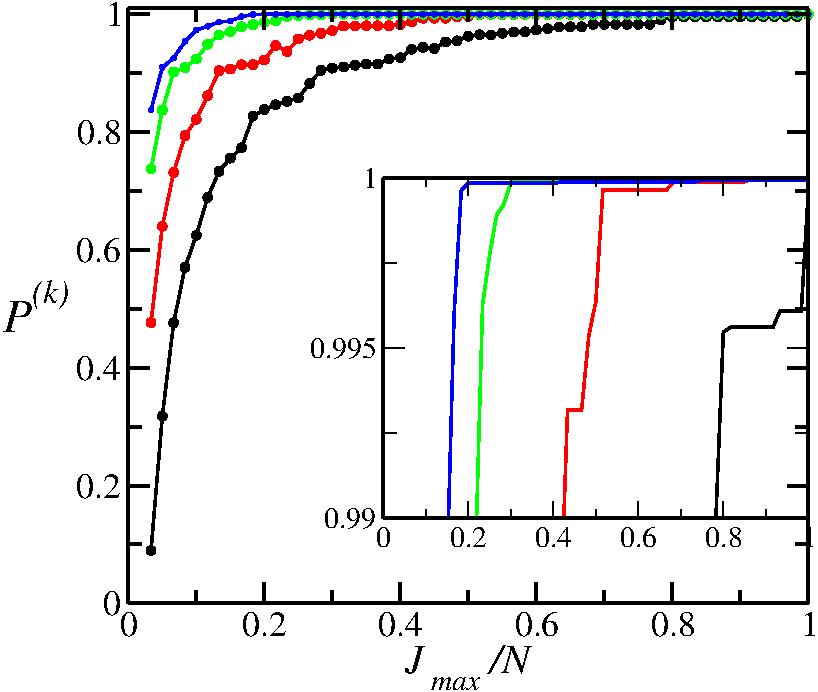
The corresponding values of the transferred population $P^{(k)}(T)$ obtained with the ECD shown in Fig. 2 are shown in Fig. 3, which also shows transferred population corresponding to arrival times $N/2$ and $N$ for a chain length $N=30$. Each point corresponds to a pair $(J_{max}^{(k)}/N,P^{(k)}(T))$, the lines are included as a guide for the eye. From the data sets it is clear that in general the ordering $P^{(k)}(T_{<})<P^{(k)}(T_{>})$ holds, where $T_{>}>T_{<}$ are two ordered arrival times. However, since $P^{(k)}(T)$ is a discrete sample of a random-like quantity for some $k$’s the ordering is reversed. All in all, the data in the figure is compatible with two reasonable physical traits, i) for a fixed $J_{max}^{(k)}$ larger arrival times results in larger transferred population, and ii) to reach a given target transferred population taking larger arrival times ensures that the target is attained for lower $J_{max}^{(k)}$.

The inset in Fig. 3 shows a detailed view of the region where the transferred population $P>0.99$. This zoom level allows us to appreciate that the transfer is of a very high quality and this is due to the excellent properties of the coefficient distribution found by the optimization method. Another feature that can be clearly observed in the inset has to do with the decreasing value of $J_{max}$ for which the transferred population reaches a given preset value, say $P=0.99$. The inset shows that this value is reached for $J_{max}\sim 0.8N$ for an arrival time equal to $N/2$, $J_{max}\sim 0.4N$ for an arrival time equal to $N$, etc. Even at this level the of magnification the largest values of $P^{(k)}$ attained for the largest values of $J_{max}^{(k)}$ explored can not be fully appreciated, since they are larger than $0.999$.

The results presented so far in the figures correspond to a chain of length $N=30$, in any case we have checked that the algorithm to find all the coefficients of a chain works correctly for chains with lengths between 10 and 90 and for various arrival times, mainly $N/2,N,2N,3N,4N$ and $5N$. In the Supplemental Material [53] we include a table with the 25 different coefficients of a chain of length $N=50$, for the times mentioned, in addition to the value of the transferred population that is obtained when a chain is assembled with these exchange coefficients. The coefficients in the Table will be used latter on.

From a theoretical point of view, that the regime where $P=1-\epsilon$ can only be attained using $J_{max}^{(k)}\approx N$ is not an impediment or a problem. For an actual implementation this trait could render the ECDs responsible of that regime useless, since changing the strength of the interaction between the components of a microscopic system on one or two orders of magnitude (depending on the length of the chain) is extremely difficult. So, in the rest of this Section we will focus on the properties of the ECDs obtained with small or moderate values of $J_{max}^{(k)}$ to evaluate them as alternative distributions that can be experimentally implemented.

One concern about the ECDs obtained for small values of $J_{max}$ is that the transferred population obtained from them could be unstable under static perturbations of the couplings, so the transferred population would be easily ruined regardless of the very good quality of the transfer produced by the unperturbed distribution.

Figure 4: Color map of the averaged transferred population as a function of the maximum value of the exchange coupling $J_{max}$ and the static disorder amplitude. Calculations were performed for a chain with $N=30$ spins and for different arrival times: (a) $T=N$, (b) $T=2N$ and (c) $T=3N$

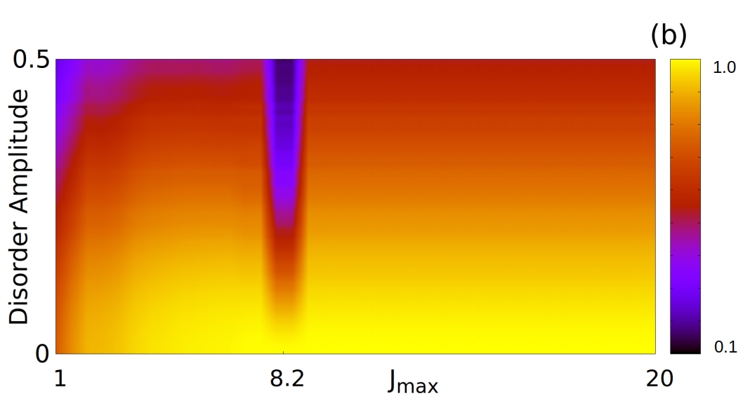
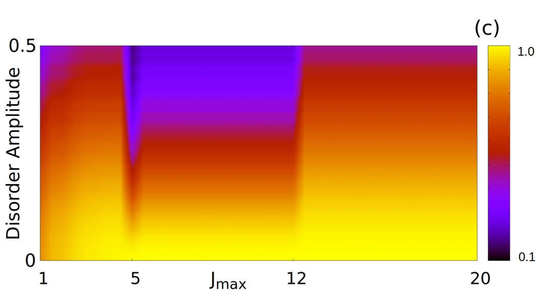
The stability of quantum state transfer in spin chains under static perturbation, or static disorder, i.e. the robustness of the transferred population when the ECDs is subject to static perturbations has been extensively studied in the literature. The static disorder is understood as a consequence of manufacturing errors of the physical system that is modeled by the spin chain. In theoretical studies the static perturbations are modeled adding a random term proportional to the coupling strength [7, 8, 45]

$$J_{i}\longrightarrow J_{i}(1+a\xi_{i}),$$ (14)

where $a$ is the strength of the disorder and $\xi$ is a random variable with zero mean and unity variance.

When static disorder is added, the transferred population averaged over realizations of the disorder is introduced as a figure of merit

$$\bar{P}=\left\langle P\right\rangle_{\xi},$$ (15)

where the average is a simple equally weighted average. This means that for a chain with $N$ spins a realization of the disorder implies that $N-1$ random numbers are generated $\{\xi_{i}^{j}\}$ and the ECD to be analyzed is changed as

$$J_{i}\longrightarrow J_{i}(1+a\xi_{i}^{j}),$$ (16)

where $1\leq j\leq n_{r}$, and $n_{r}$ is the number of realizations to be taken into account. Once a particular ECD has been generated, Eq. (16), the corresponding transferred population at arrival time $T$ is calculated, $P^{j}_{\xi}(T)$, and the averaged TP is calculated as

$$\bar{P}(T)=\frac{1}{n_{r}}\sum_{j=1}^{n_{r}}P^{j}_{\xi}(T).$$ (17)

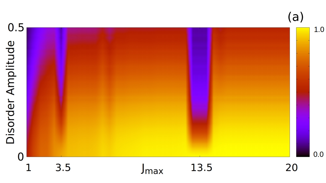
Fig. 4 shows, as color maps, the averaged transferred population (TP) as a function of $J_{ax}^{(k)}$ and the disorder strength for a chain with $N=30$ and three different arrival times. As the color map indicates, there are segments of the $J$-axis where the TP is particularly unstable, so even for very small disorder strengths the TP becomes quite poor ($P<0.9$), note the dark orange and blue fringes that appear in every map shown. Nevertheless, the segments become sparser and the fringes appear for larger disorder strengths when the arrival time considered is longer, and, for the three cases depicted there are always regions where the TP is very high and robust (the brilliant yellow regions) even for small $J$-values.

For further analyze the properties of ECDs found using the PM that produce fairly good state transfer ($P\gtrsim 0.95$) it is useful to look back at the time evolution of the population transfer, Eq. (12). So far we have studied the values reached by the population transfer at the times for which the ECD was optimized. Now we want to study the population transfer as a continuous function of time, Eq. (12). It is clear that the time-dependent functions will be different depending on the ECD that is considered but, as we will show, these different functions are closely related.

In this paper we consider that $T=\kappa N$, where $\kappa=1/2,1,2,3,\ldots$. It is clear that the population transfer obtained with an ECD optimized to show pretty good transmission at $T$ will show successive peaks at times $T_{p}=(2p+1)T$, where $p=1,2,3,\ldots$, since the time evolution should be almost periodic and the time for the state to go back and forth between the extremes of the chain is $2T$. For perfect state transfer the successive peaks of the TP are all of the same height, but for pretty good quantum state transfer the height will not be constant. The TP then, as a function of the scaled time $t/N$, will show peaks at the scaled arrival times $T^{sc}=(2p+1)\kappa$.

Figure 5: The transferred population obtained with a Heisenberg chain with $N=50$ vs the scaled time $t/N$. The TP corresponding to three different arrival times, $T=\kappa N$, with $\kappa=1/2,2$ and $5$ is shown using black, red and blue curves, respectively. Note, for instance, that for $\kappa=1/2$ the black curve shows peaks at $t/N=1/2,3/2,5/2,\ldots$ The ECD for each case was designed to achieve a target population of $0.95$. The particular values of the coupling coefficients used to assemble the transferring chains can be found in the Supplemental Material [53].

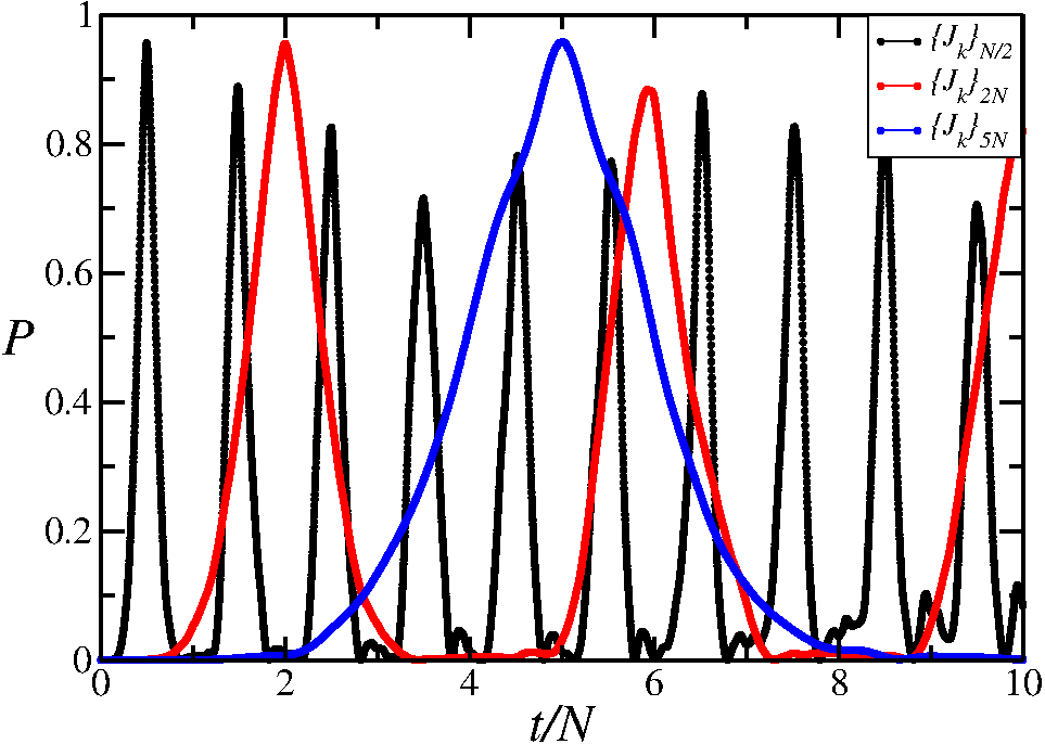
Fig. 5 shows the time evolution of the TP for three different arrival times. The corresponding ECDs were designed using the PM algorithm. The TP calculated using the ECD that is designed to produce a fairly good TP at arrival time $N/2$, the black curve, shows several peaks at scaled times $t/N=1/2,3/2,\ldots,(2j+1)/2,\ldots$, for $j\in\mathbb{N}$. The TP calculated using the ECD that must produced a peak at arrival time $2N$ shows several peaks at scaled times $2,6,10,\ldots$, while the horizontal scale only allows for a single peak of the TP calculated using the ECD that corresponds to $T=5N$. It can be seen that the peaks are broader for larger arrival times. However the apparent differences in time scale and width of the peaks corresponding to different arrival times, changing the scaling on the horizontal axis reveals a more profound relationship between them, as shown in Fig. 6.

Figure 6: a) The first five peaks of $P(\{J_{k}\}_{\kappa N},t)$ vs the scaled time $t/(\kappa N)$ for $\kappa=1/2,1,2,3,4$ and $5$, are shown using purple, magenta, black, red, green and blue curves, respectively.. The excellent superposition between the curves does not allow to distinguish between them if several peaks are included, because of this a single peak is shown in b). The particular values of the coupling coefficients used to assemble the transferring chains can be found in the Supplemental Material [53].

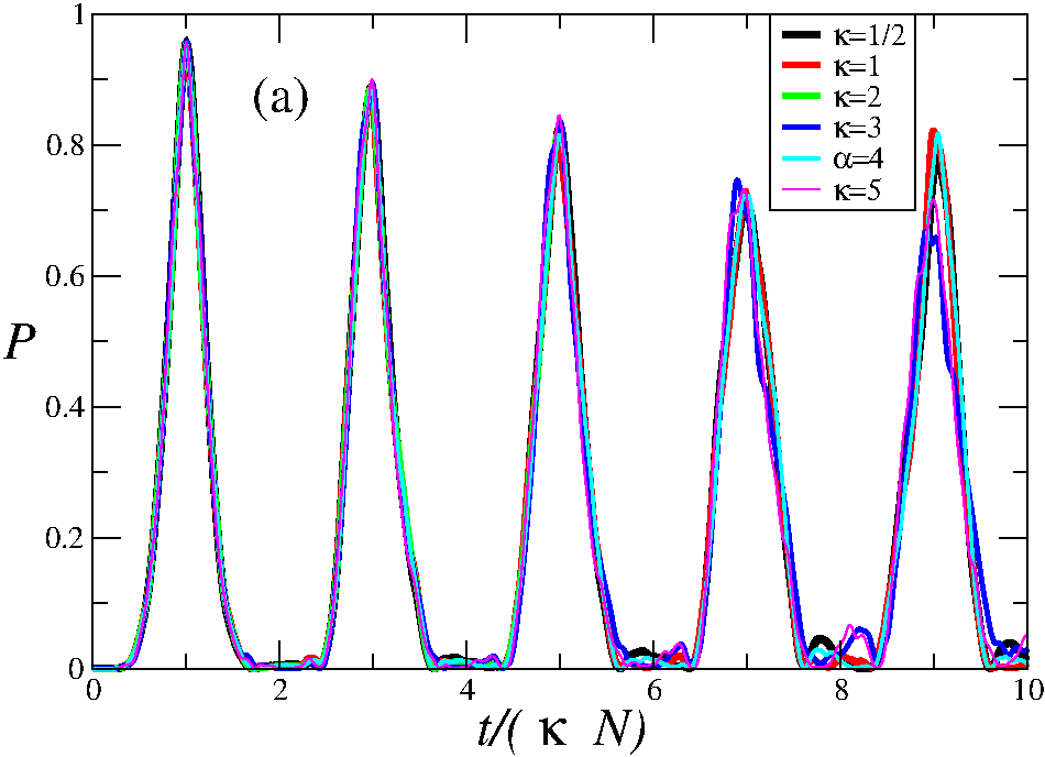
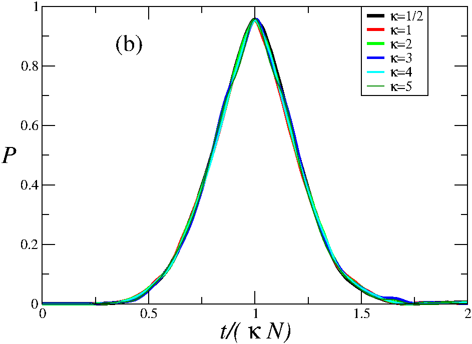
Calling $P(\{J_{k}\}_{T},t)$ the TP calculated using an ECD optimized for an arrival time $T$, Fig. 6 shows the first five peaks of $P(\{J_{k}\}_{T},t)$ vs the scaled time $t/(\kappa N)$, for $\kappa=1/2,1,2,3,4$ and $5$. The scaling is the cause the curves superposition and reveals the physics involved in the TP.

Although the ECD for each chain size and arrival time is obtained using a stochastic method, it is interesting to note that the distributions thus obtained have common features that allow deciding, according to the strength of the interactions available in a particular implementation, which ones are the arrival times compatible with these strengths.

So far, our results show that it is possible to find ECDs such that near perfect quantum state transfer is achieved for arrival times as short as $T=N/2$, if the strength of the interaction can be taken large enough. This is not what happens in actual implementations, where the range of strengths at disposal are limited by technological or physical reasons. So, it is reasonable to ask how to proceed when the range of interactions is limited. The answer, in a nutshell, is that the ECD should be sought at longer arrival times. In what follows we will show that the ECDs found using the pivot method show a relatively simple behavior that helps to determine the appropriate arrival time compatible with the range of available interactions.

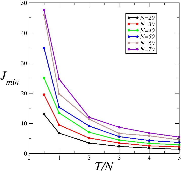
We look for the smallest hypercube that contains values of the exchange coefficients such that the transferred population reaches the target value of 0.98 and we call the corresponding side length value $J_{min}$, which depends on the length of the chain and the arrival time.

Fig. 7 shows $J_{min}$ for different chain lengths and arrival times. The values can be fitted, with a very good agreement, using an exponential function

$$J_{fit}=A(N)+B(N)e^{-C(N)\frac{T}{N}}.$$ (18)

The data and the fitting show that for fixed target TP the side length is a rapidly decreasing function of the arrival time. We think that this type of behavior is rather general if the target population is low enough (0.98, or lower) and the chain is long enough. The constants $A$, $B$ and $C$ on Eq. (18) depend on the chain length, although $C(N)$ seems to be independent of $N$ once the uncertainties in the data are taken into account.

Figure 7: The minimum length of the hypercube side necessary to obtain a population transfer of 0.98, $J_{min}$, versus the transfer time, for chains of length (from bottom to top) $N=20,30,40,50,60$ and $70$, the data is shown using black, red, green, blue, etc, solid dots, respectively. The lines are included as a guide for the eye

.

Although the results shown in figure 6 tell us that for long arrival times the intensities of the exchange interactions must all be of the same order, it is interesting to note that there are different actual physical systems in which it is possible to tune the particular values of said interactions on ranges and signs compatible with those studied in the present work. For instance, in Ref. [48] which deals with the perspectives of exchange coupled quantum dot spin chains, it is shown that positive exchange interactions can be tuned between 0 and 125 Mhz. The tunability can be used to implement SWAP operations between qubits located in adjacent quantum dots or to fix each exchange interaction coupling to a desired value. In Ref. [49] it is shown that the sign of the exchange interactions can be chosen and it can be tuned between 0 and 40 $\mu$eV. It is worth noting here that the one-excitation transfer protocol works in the same way for spin chains with all the exchange interactions positive or negative. The tunability of the exchange couplings strengths also has been demonstrated in chains of superconducting qubits see, for instance [26].

Before changing the model, it is interesting to note some of the consequences of our results with respect to the “pretty good quantum state transfer" scenario, since until now the results presented in this Section do not include the chain lengths where the regime $P=1-\epsilon$ can be proven to exist.

As well as the results shown explicitly in figures , we also obtained results for chains with even and odd number of spins, in addition to chains with length equal to powers of two . We have explored the behavior of chains with lengths between $N=10$ and $N=90$ spins, while comparing the results of chains of lengths $N=30$ and $N=31$ with $N=32$ we have not found qualitative differences between the largest transfer values accessible for any pair of chains that were compared. We also compared the results for chains with $N=60$ and $N=61$ with $N=64$ and, again, there were not discernible qualitative differences. This study was also made for different transmission times, which once again, showed that there are no qualitative differences in the largest values that can be obtained for the population transferred in chains of similar length, beyond their length being even, odd or a power of two. We think this presents fairly conclusive evidence that such a scenario is accessible for spin chains of any length with the Heisenberg Hamiltonian

It is interesting to wonder if the coupling distributions found using the pivot method allow a robust transmission of states that are initially not pure due to problems with their preparation. The Heisenberg Hamiltonian commutes with the total magnetization for any set of values that the ECDs adopt, and this can be used to estimate the population transfer in the case that the initial state is an “almost pure" state such as those used. in Nuclear Magnetic Resonance experiments.

Let us suppose that the state prepared initially can be written as

$$\rho_{i}=(1-\eta)|\psi\rangle\langle\psi|\otimes|\mathbf{0}\rangle\langle\mathbf{0}|+\eta\rho_{u},$$ (19)

where $\psi$ is the pure state that is intended to be prepared at the first site of the chain and transmitted with

$$1-\eta=\langle\psi|\otimes\langle\mathbf{0}|\rho_{i}|\psi\rangle\otimes|\mathbf{0}\rangle$$ (20)

so $\rho_{u}$ accounts for all the undesirable parts of the state that can not be eliminated because the preparation of the state is not “perfect”, and $\eta\ll 1$. Then the state after the transmission protocol can be written as

$$\rho(t)=U(t)\left((1-\eta)|\psi\rangle\langle\psi|\otimes|\mathbf{0}\rangle\langle\mathbf{0}+\eta\rho_{u}\right)U^{\dagger},$$ (21)

and the fidelity with the “expected” state is given by

$$F=\langle\psi|\mbox{Tr}_{N-1}(\rho(t))|\psi\rangle.$$ (22)

So, the transferred population of an “almost pure” state would be bounded by

$$P_{\rho}\sim P(1-\eta),$$ (23)

where $P$ is the transfer probability of the one-excitation protocol. In the paper by Di Franco et al. [46], it is discussed how to obtain perfect transfer in the event that there is no “initialization of the state to be transmitted", that is, a series of gates are applied to the ends of the chain, which allows perfect transmission of a mixed or pure state when the chain has been designed for perfect transmission in the sub space of an excitation. Our estimate of an upper bound for the transmission of poorly prepared states is consistent with the results of Di Franco et al. .

4 Results: Quantum state transfer for chains with XXZ Hamiltonian

It has been suggested by Kay [37] that some transfer properties of quantum spin chains with exchange couplings roughly equal to those of the Heisenberg chain can be studied using perturbation theory. There are several reasons for doing that study. In particular, it is of great interest to study how the transfer properties of the Heisenberg Hamiltonian, with their inherent difficulties, change towards the properties of the XX Hamiltonian, more direct to understand and for which several transfer regimes have been identified that show a direct relationship between the quality and quantity of modulation exerted on the coefficients and the quality of the transfer obtained by said modulation.

Figure 8: The transferred population $P$ vs $J_{max}$ for two chains with $N=50$ and a) $\Delta=0.8$, b) $\Delta=1.2$. The data included in both top panel correspond to arrival times $N/2$, $N,2N,3N,4N$ and $5N$. The behavior shown by the transferred population in the top panel shows that, even for the shorter arrival times, the values of the exchange couplings needed to attain $P>0.999$ are bounded by $J_{max}\lesssim 3$. In the case $\Delta=1.2$, shown in the bottom panel, the values of $J_{max}$ needed to attain high quality transfer, $P>0.99$ can become quite large for short arrival times, in a similar way to the Heisenberg case, see Fig. 3.

In this Section we apply to anisotropic Hamiltonians with $\Delta\neq 1$, see Eq. (1), the same methods that we have applied to the Heisenberg Hamiltonian in Section 3.

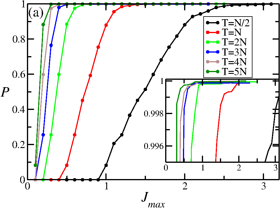
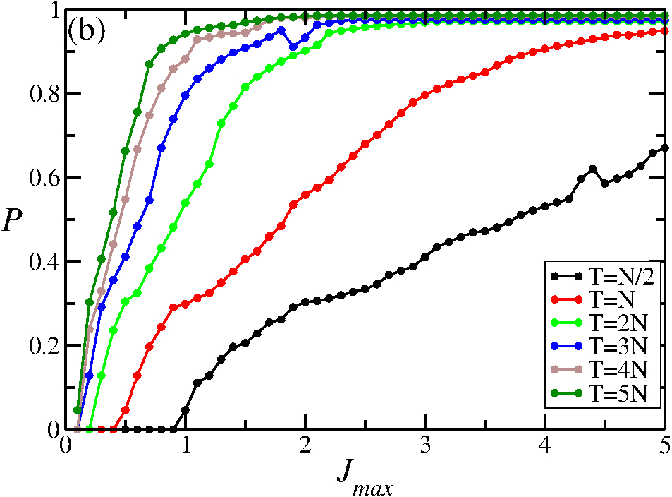
Fig. 8 shows the behavior of the TP as a function of the side length of the hypercube in whose volume the global optimization algorithm looks for the distribution of couplings that produces the largest possible transfer. The results shown in panel a) correspond to $\Delta=0.8$, while the results shown in panel b) correspond to $\Delta=1.2$, respectively.

Comparing the TP shown in the two panels of Fig. 8 it is clear that the case with $\Delta=0.8$ transfers considerably better and with the difference being greater for shorter arrival times. It is important to note that in the case of the figure corresponding to the Heisenberg Hamiltonian case, Fig. 3, the TP was shown as a function of the length of the hypercube side renormalized by the length of the chain, while in Fig. 8 it is shown as a function of the length of the side without any renormalization. The inset in Fig. 8 a) shows the TP attaining values well above 0.999 for every arrival time considered.

As was said in Section 3, when it comes to qualifying the performance of a chain built with a given distribution of coefficients, it is not only necessary to take into account the value of $J_{max}$ that limits the possible values of the coefficients and the magnitude of the transferred population, in addition the stability of the TP must be studied in the face of static disturbances.

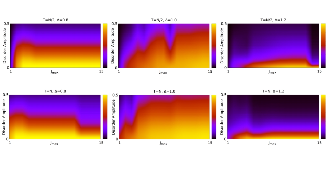
Fig. 9 shows the behavior of the averaged TP for three chains with the same length, $N=51$. The three columns, from left to right, correspond to Hamiltonians with $\Delta=0.8,1$ and $1.2$. All the necessary ECD were obtained using the PM. The top row correspond to the shorter arrival time, $T=\left[\frac{N}{2}\right]$, while the bottom row correspond to the larger arrival time $T=2\left[\frac{N}{2}\right]$. The figure summarizes quite well our findings: i) For moderate or small values of the maximum value allowed to the exchange coefficients, the figure shows values up to $J_{max}=14$, both anisotropic chains attaining larger TP when the strength of the static disorder is negligible, but the chain with $\Delta$ larger than unity is very strongly affected by disorder, making the chain useless for disorder strengths larger than $0.1$, as can be seen in the two panels in the right column and shown as a narrow fringe of brilliant yellow and light orange, the two colors that correspond to a high-quality transfer. ii) Conversely, the TP obtained using the chain with $\Delta=0.8$ is weakly affected by static disorder, presenting a TP of a very high quality, as is depicted by the broad fringe of brilliant yellow and light orange that appear in both panels in the left column. iii) Finally, the Heisenberg chain is very resistant to static disturbances, even for a range of intensities of the disorder even greater than the chain with $\Delta<1$. However, the first type of chain does not reach as high transmission values as the second one for these values of $J_{max}$.

The behavior of the TP shown in the right and left columns of Fig. 9 can be, in practice, translated to any value of $\Delta>1$ and $\Delta<1$, respectively. Chains whose Hamiltonians have $\Delta<1$ and ECDs optimized using the PM show excellent quantum state transmission, with very high values of $P$ and are very resilient against static disorder. Moreover, the ECDs obtained for short arrival times are bounded by $J_{max}\sim\mathcal{O}(1)$ independently of the chain length, at least for $N<100$ the range of chain lengths that we have explored. In a sense, it is reasonable to say that chains with Hamiltonians with $\Delta<1$ are XX-like in as much as their quantum state transfer properties are involved.

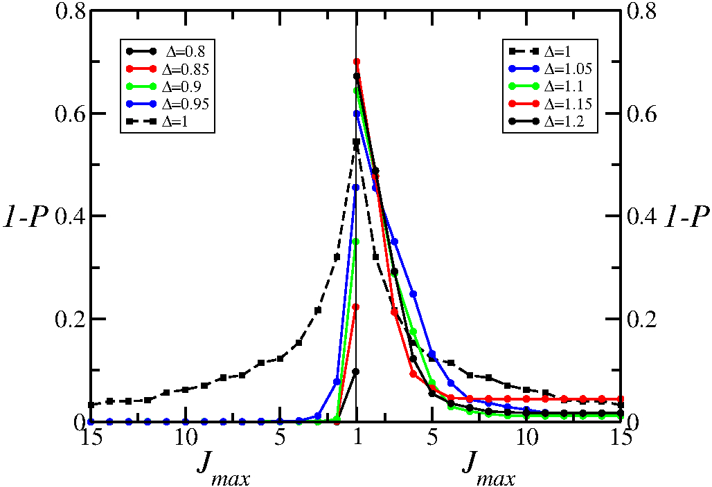
The rapid departure of the behavior of the transferred population when the Hamiltonian of the chain has $\Delta<1$, from the behavior observed when the chain obeys the Heisenberg Hamiltonian can be seen in the Fig. 10. The figure shows $1-P$ as a function of $J_{max}$, in the left panel the data corresponds to chains with $\Delta\leq 1$, while the right panels shows the data corresponding to chains with $\Delta\geq 1$. The color of the data points and curves in both panels have been chosen so that the chains at the same "distance" from the isotropic case have the same color, so the data for the chains with $\Delta=0.8$ and 1.2 are shown with black points, for the chains with $\Delta=0.85$ and 1.15 with red points, and the following with green and blue dots. The resemblance with “ $\lambda$-point” plot is striking.

The value of $J_{max}$ for which the PT reaches a given target value for chains with $\Delta>1$ is an increasing function of $1/(1-\Delta)$. To determine this function, it would be necessary to study much longer chains, with the consequent expenditure in computing time, anyway for finite chains there can not be any divergences so, in the worst case scenario $J_{max}$ grows up to values $\mathcal{O}(N)$ for arrival times $\mathcal{O}(N)$.

Figure 9: Color map of the averaged TP as a function of the maximum value of the exchange coupling and the static disorder amplitude. Results were obtained for a chain with $N=51$ spins, two different arrival times $T=N/2$ and $T=N$ and three different values of the anisotropy parameter $\Delta=0.8,1.0$ and $1.2$.

Figure 10: $1-P$ vs $J_{max}$ for chains with $N=61$ and for an arrival time $T=60$. The transferred population is shown in this way to emphasize the quite different behavior observed by the transmission in chains with $\Delta<1$,whose data is shown in left half of the figure, from the one observed in chains with $\Delta>1$, whose data is shown in the right half of the figure. Note that the values of the variable $J_{max}$ increase from 1 (in the middle of the horizontal axis) to 15 (at the left and right extremes of the horizontal axis) . The same colors are used for data that correspond to chains with the same $\Delta^{\prime}$, with $\Delta=1\pm\Delta^{\prime}$. Note that $\Delta^{\prime}=0.2$ is shown with black dots, $\Delta^{\prime}=0.15$ with red dots and so on.

Even when the averaged transferred population could be very high, it is logical to ask what the "worst case" scenario is like. This question is particularly important in experiments in which only a single-shot transmission attempt is made and there are no error correction algorithms available. To obtain the worst case scenario, it is necessary to calculate numerous realizations of the disorder and keep track of the smallest transferred population.

In the Supplemental Materials we have included a figure comparing the averaged transferred population and the worst transferred population as functions of the disorder amplitude and for different chains . We also included a plot showing the standard deviation of the transferred population. All in all, the results, although preliminary, show that for moderate disorder amplitude the Heisenberg isotropic chain is the better option as a transmission channel and that the statistics of transferred population in quite different between the different model chains. Other authors also have studied the statistics of the quantum state transfer, in particular G. Nikolopoulos [52]. In this paper it is shown that the minimal fidelity is equal to the worst population transferred for $P>0.5$. The regime of interest is found for values of $P>0.5$, so the worst case TP is a good qualifier of the transfer process.

5 Discussion and Conclusions

If the strength of the couplings is not an issue, which in a microscopic system does not seem realistic, it is possible to design chains with the Heisenberg Hamiltonian that transfer an excitation between the ends of the chain with very good probability at times as short as $N/2$ or $N$. In any case, if the intensity of the couplings is limited (at most couplings less than or equal to two), considering arrival times of the order of 4 or $5N$ is recommended. This last point is of particular importance for possible practical implementations. In the same sense, if the spin Hamiltonian is an effective approximation for the low energy spectrum of a given physical system, it is advisable to look for a physical regime for the original system in which the resulting model Hamiltonian is anisotropic with $\Delta<1$.

Based on the results shown Fig. 9 about the behavior of the averaged TP we analyzed the stability of the transmission process for relatively short arrival times, $N/2$ and $N$. We also obtained results for longer times and the same chain length $N=50$, which are not consigned to any figure, and the conclusion drawn in Section 4 holds, that is, chains with $\Delta<1$ transfer excitations with greater probability than chains with $\Delta=1$ , which in turn transmits better than those with $\Delta>1$. For times $4N$ or $5N$, the chains with $\Delta\leq 1$ reach very high values of the transmission probability ($P>0.9998$), but in those with Heisenberg’s Hamiltonian the averaged TP decay faster than on the chains with $\Delta<1$ when the intensity of the disorder is increased . The chains with $\Delta>1$ never reach the highest levels of quality in transmission than are attained by chains with $\Delta\leq 1$ and are severely affected by static disorder.

The linear scaling of the transferred population, Fig. 6, is noteworthy for a number or reasons, i) the ECD which are used to obtain the PT are bounded by a quantity that changes non-linearly with the arrival time, ii) each ECD is obtained independently for each time, and iii) the TP is a nonlinear functions of the couplings. So far we have not reached a conclusion about how to look for scaling properties in the eigenvalues of the Hamiltonian of the chain and the coefficients of the eigenvectors that enter into the calculation of the transferred population.

The results found show us that the ECDs found are relatively robust but, even in the best case, if there is a static disorder present with a strength larger than $10\%$, these distributions no longer offer a valid alternative to build chains of spins that serve for the transfer of quantum states. In the case of chains with XXZ Hamiltonians with $\Delta>1$ even smaller disorder strengths render useless the chain as a transmission channel. Some of these features can be better appreciated in the figure that is included in [53]. So, from the quantum state transfer point of view the regime of interest can be found for $a<0.1$. Notwithstanding this, the patterns observed in Fig. 4 and 8, which can be clearly appreciated for disorder strengths larger than $0.1$, seem to indicate that there are different dynamical regimes. The propagation of information can show very different speed bounds in disordered spin chains and be suppressed for strong enough disorder see, for instance, Ref. [47]. Assert that the observed patterns are due to this requires more research, which is being carried out, and depends on the study of the scaling properties of the matrix elements of the evolution operator associated with the problem.

Fig. 3 shows that, apparently, the system is more robust for smaller transfer times than for larger ones, at least for some intervals of the variable $J_{max}$. This is so, in part, because the figure shows the transfer probability against a single parameter $J_{max}$ while the detailed behavior of $P$ depends on the whole set of exchange couplings. All the exchange couplings are bounded by $J_{max}$, but this bound does not give a detailed information about the distribution of the $J_{i}$. Stochastic optimization methods can be trapped in a "good" minimum and do not provide information about the landscape topology of the valley where the “good" minimum lies and the width of this valley is what determines the robustness of the transfer process against disorder. All this results in that the exchange coupling distributions found for short times are more robust against disorder than the exchange coupling distributions found for longer times, in certain intervals of the variable $J_{max}$, see Fig. 3 a), b) and c).

The transferred population $P$ is a probability, but the information that it shows is not enough to quantify large changes in the ECDs. An interesting quantity to study is the probability of transferring an excitation from a given site of the chain, $m$, to any other site of the chain, $n$, given by $P_{mn}(J_{max})$, where $J_{max}$ is the value which was used to determine the ECD. It is clear that the TP is given by $P_{1,N}$. Studying the statistical divergence [50] between two probability distributions $D(\{P_{nm}(J_{max})\},\{P_{nm}(J_{max}^{\prime}\})$, it is possible to determine their properties and how susceptible they are to disorder. We use $\{P_{nm}(J_{max})\}$ to denote the set of probabilities with $1\leq m,n\leq N$ . We have carried out preliminary studies using the Renyi divergence [51], $D_{1/2}$ , and verified that the divergence reproduces the patterns structure observed in Fig. 3 and Fig. 6.

Fig. 3 shows vertical regions, for instance in Fig. 3 c) there are three clearly appreciable regions whose limits are $J_{max}\leq 5$, $5\leq J_{max}\leq 12$ and $12\leq J_{max}$. These limits correspond, exactly, with plateaus observed in the coupling coefficient distributions. In the different regions it can be observed that the susceptibility to disorder is different, as the color map indicates. For example, again in Fig. 3c), it can be seen that the distributions of coupling coefficients such that $5\leq J_{max}\leq 12$ are more susceptible to disorder than the distributions at both sides. In the $5\leq J_{max}\leq 12$ region the propagation of excitations is strongly suppressed by the increase in the strength of the disorder. In regions where the system is not very susceptible to disorder, the excitation that is initially located at one end of the chain spreads over a large portion of the chain and refocuses at the time of transmission. In areas that are strongly affected by the disorder, the initial excitation spreads over a few sites in the chain and the refocusing hardly occurs, which results in a very poor transferred population. This analysis was carried out calculating the inverse participation ratio, a quantity that is commonly used to analyze transport properties in disordered systems and quantum state transmission, see Ref. [6] and references therein.

The coupling distributions resulting from the application of the PM to chains with the Heisenberg Hamiltonian show that it is possible to reach a regime where $P=1-\epsilon$ for chains of any length, not only for chains whose length is a power of 2, for arrival times of the order of N as long as the magnitude of the couplings is not bounded. At present we cannot affirm whether the regime for chains with lengths that are powers of two is the same as for chains of arbitrary length. We will implement more numerical calculations to try to elucidate this issue.

Acknowledgments The authors acknowledge partial financial support from CONICET (PIP11220150100327, PUE22920170100089CO). O.O and P.S. acknowledges partial financial support from CONICET and SECYT-UNC.

Comparison between the averaged and "worst" transferred populations

Figure 11: The average transferred population (continuous line) and the "worst case" in a single experiment (dashed line) versus the strength of the static disorder. The data shown was obtained for chains of length $N=51$, $J_{max}=14$ and $N_{r}=10000$ realizations of the static disorder. See the text for details.

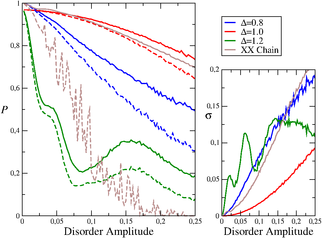
The figure above shows the average transferred population versus the strength of the static disorder (solid lines) for chains of length $N=51$. The arrival time is $T=N$. The red line corresponds to a Heisenberg chain, $\Delta=1$, while the blue and green lines correspond to $\Delta=0.8$ and $1.2$, respectively, while the brown lines correspond to a spin chain whose dynamics is governed by the XX Hamiltonian, i.e. $\Delta=0$. . The dashed lines correspond to the "worst case", that is, the minimum population transfer obtainable in a single experiment. It can be observed that without static disorder the $\Delta<1$ chain has a better performance than $\Delta=1$ and $\Delta>1$, but that for disorder strengths larger than 0.05 the Heisenberg chain is clearly superior as a transmission channel, being the distance between the average and the "worst case" always smaller for that chain.

For comparison reasons we have also included results for an XX chain which are depicted using brown lines, despite that the main interest of the manuscript are chains with XXZ Hamiltonians. It is interesting to note that, with respect to the averaged transferred population, the XX TP shows three different regimes. In the first one its TP is indistinguishable from the TP obtained for the $\Delta<1$, for disorder amplitudes $a\lesssim 0.05$. For larger values of the disorder amplitude and up to $a\approx 0.075$ the TP of the XX chain remains larger or comparable to the Heisenberg case, while for $a>0.075$ the TP of the Heisenberg chain is always larger than all the other cases.

From the results shown for the averaged TP it could be concluded that, if it is known a priori which is the expected amplitude of disorder and it is possible to implement any type of chain, then the most suitable transmission channels are the XX chain or the Heisenberg chain. Nevertheless, as shown by the worst case curves, the TP of the XX chain shows by far the worst “worst case”, see the brown dashed curve in the figure. Moreover, even though that all the curves were obtained using the same number of disorder realizations, it is clear from the large fluctuations shown by the worst case for the XX chain that the statistics of the TP of the XXZ cases is quite different from that of the XX chain. The large fluctuations of the worst case are not as surprising since it is not a good statistical estimator as the standard deviation or the average are. The convergence of the worst case TP to its true value is quite slower in the XX case when compared with the other cases.

The right panel shows the statistical standard deviation of the transferred population. The color code is the same as that used in the panel on the left. Again it can be seen that the dispersion of the values in the case of the Heisenberg chain is less than for the other two chains. If $P_{i}$ is the transferred population obtained for the $i-$th realization of the disorder, the averaged transferred population was introduced in the main text

$$P=\left\langle P\right\rangle_{\xi}=\frac{1}{M}\sum_{i=1}^{N_{r}}P_{i},$$ (24)

where $N_{r}$ is the number of realizations considered, the minimum transferred population is given by

$$P_{min}=\min_{i}(P_{i}),$$ (25)

and the statistical standard deviation of the transferred population can be calculated as

$$\sigma=\frac{1}{N}\sum_{i=1}^{N_{r}}(P_{i}-P)^{2}.$$ (26)

Here, it is worth to point out that the standard deviation of the XX chain is quite close to the anisotropic $\Delta<1$ case.

Exchange coupling distribution for a Heisenberg Chain with $N=50$

In the following we give a table with the numerical values of all the quantities used in Figures 5 and 6 of the main text. They correspond to an Isotropic Heisenberg model with $N=50$ sites , and transfer times $T=\kappa\,N$, with $\kappa=1/2,\;1,\;2,\;3,\;4,$ and $5$.

$\kappa$	$1/2$	1	2	3	4	5
$P$	0.9557	0.9531	0.9550	0.9564	0.9530	0.9573
$J_{max}$	19.0	9.5	4.5	3.5	2.5	2.0
$J_{1}$	0.39944	0.20749	0.10238	0.067054	0.051485	0.041025
$J_{2}$	10.848	4.2954	1.9585	3.3773	1.0095	0.92646
$J_{3}$	9.6847	2.9696	2.0284	0.60075	0.93922	0.3956
$J_{4}$	18.273	8.5247	4.2234	2.7508	1.413	1.2784
$J_{5}$	7.2718	7.3141	2.4777	2.1946	1.2422	1.7371
$J_{6}$	7.4144	4.1991	2.2276	3.4409	1.9408	1.7506
$J_{7}$	12.375	6.3237	2.3133	2.2059	1.1415	1.7628
$J_{8}$	16.283	5.2431	3.4801	2.1465	1.1807	1.6982
$J_{9}$	14.393	6.6373	3.3664	0.92832	2.0173	0.42639
$J_{10}$	8.6577	7.2860	3.8836	1.4471	1.5871	1.7395
$J_{11}$	15.283	5.8929	2.9566	2.2067	1.6632	1.0526
$J_{12}$	15.390	7.6673	2.7579	3.1806	1.7769	1.9995
$J_{13}$	18.846	7.1904	4.1133	3.0605	1.9180	1.9632
$J_{14}$	12.222	7.6271	4.1504	3.3954	1.5966	1.8553
$J_{15}$	17.139	7.5777	3.8859	3.4753	1.7934	1.9868
$J_{16}$	18.045	6.8020	4.5000	3.5000	2.1608	1.9033
$J_{17}$	14.860	9.1612	3.2385	3.5000	1.9981	1.8423
$J_{18}$	18.980	6.7268	4.5000	2.2440	2.1971	1.7891
$J_{19}$	19.000	7.9982	4.2445	3.1035	1.6376	1.6230
$J_{20}$	13.197	8.9228	3.7993	1.9047	2.5000	1.1124
$J_{21}$	19.000	7.9298	3.9049	3.2019	1.8421	1.6021
$J_{22}$	10.844	6.5456	2.9507	1.8041	1.8788	1.3331
$J_{23}$	12.583	3.6055	3.9359	2.8118	1.0171	0.9925
$J_{24}$	13.037	5.6579	1.4901	2.6015	0.87489	1.3820
$J_{25}$	5.645	3.7480	3.9673	1.5246	2.3294	1.6348

Table 1: Values of $P$ and $\{J_{i}\}$ obtained with the pivot method for global optimization inside an hypercube of size $J_{max}$ for $N=50$, used to made Figures 5 and 6 of the paper.

References

- [1] G.M. Nikolopoulos and I. Jex (Edts.), Quantum State Transfer and Network Engineering, Springer-Verlag Berlin Heidelberg 2014
- [2] S. Bose, Phys. Rev. Lett. 91, 207901 (2003).
- [3] S. Bose, Contemporary Physics, 48:1, 13-30 (2007)
- [4] M. Christandl, N. Datta, A. Ekert, and A. J. Landahl, Phys. Rev. Lett. 92,187902 (2004).
- [5] M. Christandl, N. Datta, T. C. Dorlas, A. Ekert, A. Kay, and A. J. Landahl, Phys. Rev. A 71, 032312 (2005).
- [6] A. Zwick and O. Osenda, J. Phys. A: Math. Theor. 44 105302 (2011).
- [7] A. Zwick, G. A. Álvarez, J. Stolze, and O. Osenda, Phys. Rev. A 84, 022311 (2011).
- [8] A. Zwick, G. A. Álvarez, J. Stolze and O. Osenda, Quantum Information and Computation 15, 0582 (2015).
- [9] Man-Hong Yung, Phys. Rev. A 74, 030303(R) (2006).
- [10] D. Burgarth and S. Bose, Phys. Rev. A 71, 052315 (2005).
- [11] D. Burgarth and S. Bose, New Journal of Physics 7, 135 (2005).
- [12] L. Banchi, T. J. G. Apollaro, A. Cuccoli, R. Vaia, and P. Verrucchi, Phys. Rev. A 8̱2, 052321 (2010).
- [13] L. Banchi, T. J. G. Apollaro, A. Cuccoli, R. Vaia and P. Verrucchi, New J. Phys. 13, 123006 (2011).
- [14] X. Wang, A. Bayat, S. G. Schirmer, and S. Bose, Phys. Rev. A 81, 032312 (2010).
- [15] V. Jurdjevic and H. J. Sussmann, J. Diff. Eqn. 12, 313 (1972).
- [16] D. Burgarth, S. Bose, C. Bruder, and V. Giovannetti, Phys. Rev. A 79, 060305(R) (2009).
- [17] V. Ramakrishna, M. V. Salapaka, M. Dahleh, H. Rabitz, and A. Peirce, Phys. Rev. A 51, 960 (1995).
- [18] X. Wang, D. Burgarth, and S. Schirmer, Phys. Rev. A 94, 052319 (2016).
- [19] D. Burgarth, K. Maruyama, M. Murphy, S. Montangero, T. Calarco, F. Nori, and M. Plenio, Phys. Rev. A 81, 040303(R) (2010).
- [20] S. Yang, A. Bayat, S. Bose, Phys. Rev. A 82, 022336 (2010) .
- [21] R. Heule, C. Bruder, D. Burgarth, and V. M. Stojanovic, Phys. Rev. A 82, 052333 (2010).
- [22] D. Stefanatos and E. Paspalakis, Phys. Rev. A 99, 022327 (2019).
- [23] G. Watanabe, Phys. Rev. A A 81, 021604(R) (2010).
- [24] V. Kostak, G. M. Nikolopoulos, and I. Jex, Phys. Rev. A 75, 042319 (2007)
- [25] D. M. Zajac, T. M. Hazard, X. Mi, E. Nielsen, and J. R. Petta, Phys. Rev. Applied 6, 054013 (2016).
- [26] X. Li, Y. Ma, J. Han, Tao Chen, Y. Xu, W. Cai, H. Wang, Y.P. Song, Zheng-Yuan Xue, Zhang-qi Yin, and Luyan Sun, Phys. Rev. Applied 10, 054009 (2018)
- [27] Jingfu Zhang, Gui Lu Long, Wei Zhang, Zhiwei Deng, Wenzhang Liu, and Zhiheng Lu, Phys. Rev. A 72, 012331 (2005); P. Cappellaro, C. Ramanathan, and D. G. Cory, Phys. Rev. A 76, 032317 (2007); J. Zhang, M. Ditty, D. Burgarth, C. A. Ryan, C. M. Chandrashekar, M. Laforest, O. Moussa, J. Baugh, and R. Laflamme, Phys. Rev. A 80, 012316 (2009)
- [28] N. J. S. Loft et al New J. Phys. 18 045011 (2016).
- [29] L. Banchi, A. Bayat, P. Verrucchi, and S. Bose, Phys. Rev. Lett. 106, 140501 (2011).
- [30] R. J. Chapman, M. Santandrea, Zixin Huang, G. Corrielli, A. Crespi, Man-Hong Yung, R. Osellame and A. Peruzzo, Nat. Comm. 7, 11339 (2016).
- [31] Yadav P. Kandel, Haifeng Qiao, Saeed Fallahi, GeoffreyC. Gardner, MichaelJ. Manfra, JohnM. Nichol, Nature 573 (2019) 553.
- [32] D.S.Acosta Codena, S.S.Gómez, A.Ferrón, O.Osenda, Physics Letters A 387 127009 (2021).
- [33] X.P. Zhang, B. Shao, S. Hu, J. Zou, L.A. Wu, Ann. Phys. 375 (2016) 435–443.
- [34] J. Gong and P. Brumer, Phys. Rev. A 75, 032331 (2007).
- [35] M. Murphy, S. Montangero, V. Giovannetti, T. Calarco, Phys. Rev. A 82, 022318 (2010).
- [36] U. Farooq, A. Bayat, S. Mancini, S. Bose, Phys. Rev. B 91, 134303 (2015).
- [37] Alastair Kay - arxiv-1906.06223 perfect and pretty good state transfer for field-free Heisenberg chains
- [38] Alastair Kay, International Journal of Quantum Information Vol. 8, No. 4 (2010) 641-676
- [39] Leonardo Banchi, Gabriel Coutinho, Chris Godsil, and Simone Severini, Journal of Mathematical Physics 58, 032202 (2017) ,
- [40] Christopher M. van Bommel, Pretty Good State Transfer and Minimal Polynomials, arXiv:2010.06779v1
- [41] Xiao-Ming Zhang, Zi-Wei Cui, Xin Wang, and Man-Hong Yung, Phys. Rev. A 97, 052333 (2018).
- [42] P. Serra, A. F. Stanton and S. Kais, Phys. Rev. E 55, 1162 (1997).
- [43] P. Serra, A. F. Stanton, S. Kais and R. E. Bleil, J. Chem. Phys. 106, 7170 (1997).
- [44] W.H. Press, S.A. Teukolsky, W.T. Vetterling and B.P. Flannery, Numerical Recipes in Fortran 77, 2nd ed., Cambridge University Press, Cambridge (1996).
- [45] D. Petrosyan, G. M. Nikolopoulos, and P. Lambropoulos, Phys. Rev. A 81, 042307 (2010).
- [46] C. Di Franco, M- Paternostro and M. S. Kim, Phys. Rev. Lett. 101, 230502 (2008).
- [47] C- K- Burrell and T. J. Osborne, Phys. Rev. Lett. 99, 167201 (2007).
- [48] Y. P. Kandel, H. Qiao, and J. M. Nichol, Appl. Phys. Lett. 119, 030501 (2021).
- [49] F. Martins, F. K. Malinowski, P. D. Nissen, S. Fallahi, G. C. Gardner, M. J. Manfra, C. M. Marcus, and F. Kuemmeth, Phys. Rev. Lett. 119 227701 (2017).
- [50] S. Eguchi, Hiroshima Math. J. 15 341 (1985).
- [51] T. V. Erven, P. Harremoës, IEEE Transactions on Information Theory. 60, 3797 (2014).
- [52] G. M. Nikolopoulos, Phys. Rev. A 87, 042311 (2013)
- [53] Supplemental Material