July \jdsyear2020 \jdsvolumexx \jdsissuexx \jdsdoixx.xxxx/xxxxxxxxx \jdsreceivedApril, 2020 \jdsacceptedMay, 2020 11affiliationtext: Data and Statistical Sciences, AbbVie Inc., Illinois, USA 22affiliationtext: Department of Biostatistics, School of Public Health, University of Michigan, Ann Arbor, Michigan, USA
BDNNSurv: Bayesian Deep Neural Networks for Survival Analysis Using Pseudo Values
Abstract
There has been increasing interest in modeling survival data using deep learning methods in medical research. In this paper, we proposed a Bayesian hierarchical deep neural networks model for modeling and prediction of survival data. Compared with previously studied methods, the new proposal can provide not only point estimate of survival probability but also quantification of the corresponding uncertainty, which can be of crucial importance in predictive modeling and subsequent decision making. The favorable statistical properties of point and uncertainty estimates were demonstrated by simulation studies and real data analysis. The Python code implementing the proposed approach was provided.
keywords:
Deep learning; Neural networks; Survival outcome; Pseudo probability; Bayesian; Automatic differentiation variational inference.1 Introduction
Time-to-event (TTE) modeling is one of the most widely used statistical analysis tools in health data science applications. TTE analysis deals with outcomes that consist of the time to some event (death, occurrence of a disease, etc.). We refer this time as survival time hereafter. TTE analysis is unique because the outcome of interest is not only whether an event has occurred or not (a binary outcome), but also when that event occurred (a continuous outcome). Furthermore, the outcome data maybe censored (i.e., incomplete observations), in particular right-censored; for example, patients may be lost to follow-up without experiencing the event. Thus, traditional methods, such as logistic or linear regression, can not be used to handle censored survival data.
Using neural networks to predict time-to-event has recently gained considerable attentions when there is a larger number of covariates (Martinsson, 2016; Katzman et al., 2018; Ching et al., 2018; Zhu et al., 2016; Gensheimer and Narasimhan, 2019; Fotso, 2018; Lee et al., 2018; Luck et al., 2017; Giunchiglia et al., 2018; Zhao and Feng, 2020). Neural networks is one of the most popular machine learning algorithms. It has been shown that neural networks outperform other algorithms in predictive modeling for certain tasks. The neural networks can outperform (1) widley used classical methods, e.g., Weibull regression (Martinsson, 2016), Cox proportional hazards model (Katzman et al., 2018; Gensheimer and Narasimhan, 2019; Fotso, 2018; Lee et al., 2018; Luck et al., 2017; Giunchiglia et al., 2018), and (2) more recently developed statistical learning/machine learning methods, such as LASSO, ridge, minimax concave, and both and norm penalty (Ching et al., 2018; Zhu et al., 2016; Giunchiglia et al., 2018), random forest regression (Katzman et al., 2018; Ching et al., 2018; Zhu et al., 2016; Lee et al., 2018; Giunchiglia et al., 2018), boosting based methods(Ching et al., 2018; Lee et al., 2018). Moreover, the neural networks can handle not only high-dimensional but also unstructured data like medical images (Zhu et al., 2016). In the TTE analysis, different types of neural networks, including deep neural networks (DNN), convolutional neural networks (Zhu et al., 2016) and recurrent neural networks (Martinsson, 2016; Giunchiglia et al., 2018) have been adopted. Besides different network architectures, various loss functions have been used based on the Weibull regression model (Martinsson, 2016), the Cox proportional hazards model (Katzman et al., 2018; Ching et al., 2018; Zhu et al., 2016) or the discrete survival model (Gensheimer and Narasimhan, 2019; Fotso, 2018; Lee et al., 2018; Luck et al., 2017; Giunchiglia et al., 2018; Zhao and Feng, 2020).
The model built upon the Weibull regression assumes a parametric form of the distribution of survival time. The semi-parametric Cox proportional hazards regression instead studies effects of covariates on the hazards and relies on the proportional hazards (PH) assumption; that is, the effect of a unit increase in a covariate is multiplicative with respect to the hazard rate. However, the quantity of direct interest sometimes is the survival probability rather than hazards. Furthermore, the PH assumption maybe questionable especially when the number of covariates is large, since every covariate needs to satisfy the PH assumption. Both parametric and semi-parametric models do not perform well when the model is mis-specified.
Recently, a flexible, simple deep neural network model was proposed in the survival setting (Zhao and Feng, 2020). This approach consists of two steps. The first step is to compute the jackknife pseudo survival probabilities in the discrete-time survival framework, and substitute the survival times with censoring by these pseudo probabilities. By using the pseudo values, the analysis for censored survival data is reduced to a regression problem with a quantitative response variable, which greatly facilitates the use of deep learning methods. In the second step, standard deep neural networks can be directly applied, which avoids the difficulty of designing a special cost function for the censored data.
In this paper, we extended the work in zhao2019 to implement the two-step network model in a Bayesian framework. The framework enables quantification of the uncertainty of the predicted survival probability, which is an appealing feature in predictive modeling. The uncertainty is inherent in machine learning due to measurement error in data, randomness of estimated parameter values and model inadequacy. A key characteristic that distinguishes statistically rigorous approaches to prediction from other approaches is the ability to accurately quantify uncertainty of a prediction. The quantification of uncertainty can be harnessed to potential inspection of over-fitting, accurate comparison of treatment efficacy/effectiveness and identification of difficult diagnostic cases for further evaluation (ghahramani2015; leibig2017; kendall2017; wager2014).
The remainder of this article is organized as follows. In section 2, we describe the details of our Bayesian deep neural networks model for survival analysis (BDNNSurv). In section 3, we present results from a simulation study to evaluate our proposed method. In section 4, we demonstrate the application of our method to a prospective multicenter cohort study for cardiovascular disease. We conclude this paper with discussions in section 5.
2 Methodology
Following our previous work in zhao2019, we substituted the survival times with pseudo survival probabilities and then implemented the standard deep neural networks model for a regression problem with a quantitative outcome. In this section, we first briefly introduce the pseudo values calculation and then describe the BDNNSurv approach.
Let be the survival time for subject , be the censoring time, be the observed survival time, and be the censoring indicator. We assumed that survival times and censoring times are independent. Let denote the -dimensional covariates. The pseudo-observations approach (Andersen:2003; Klein:2005; Klein:2007; Andersen:2010; Tayob:2017; Xiang:2012; ZhaoMurray:2020) provides an efficient and straightforward way to study the association between the covariates and survival outcome in the presence of censoring.
Note that due to censoring, the survival probability at a specific time cannot be directly modeled as a binary outcome on () using a generalized linear model (GLM) with a logit link, In the presence of censoring, is not observed for all subjects. In this case the Kaplan-Meier (KM) estimator can be used to estimate the survival probability at any given time point. Based on the jackknife idea, a pseudo survival probability is computed for each (censored and uncensored) subject. For the subject, the pseudo survival probability is computed by
| (1) |
where is the KM estimator of using all subjects and is the KM estimate using sample size of by eliminating the subject. Then () are used as a continuous response variable in the standard regression analysis, regardless of censoring or not.
We applied the deep neural network to model the pseudo survival probability. Let be a layer of a deep neural network, ; be the dimension of input layer; be the number of neurons in layer ; be an activation function; be an affine linear map defined by a matrix and an affine part via . Then given by
is a deep neural network (DNN). The input layer is layer 0 with and the output layer has one dimension with . The neural network is a function that maps input covariates to a desired target value , the corresponding pseudo survival probability. When . Figure 1 shows an architecture of a neural network with two fully connected hidden layers.
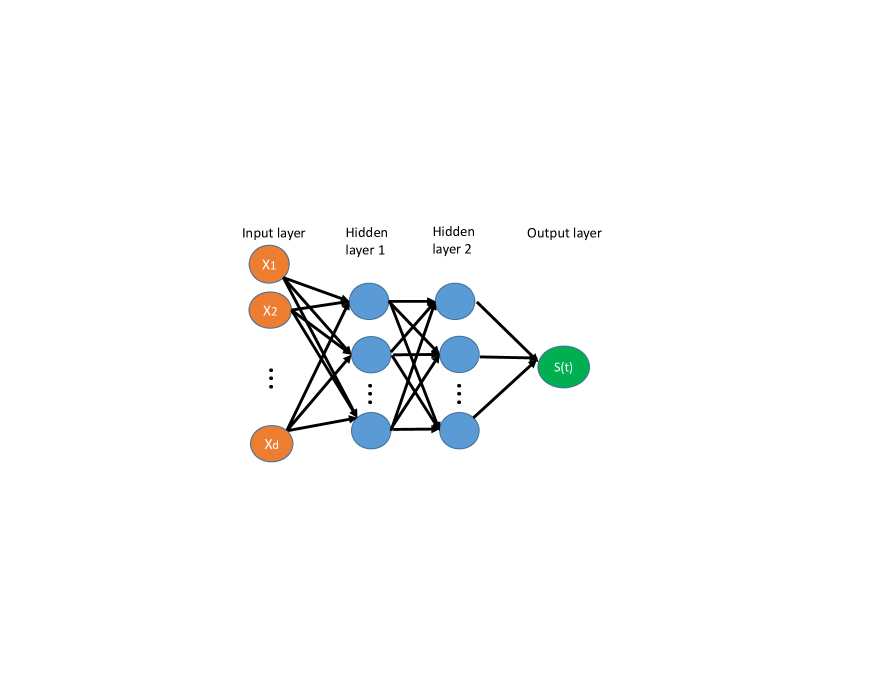
To build a DNN, the architecture, including , are pre-determined by using, for example cross-validation. The parameters of affine transformation are traditonally obtained by minimizing the loss function or the objective function. For example, the loss function in zhao2019 for the numeric response of pseudo probabilities is the mean squared error. The optimization(minimization) is done using gradient descent. A fast algorithm for computing gradients is backpropagation (nielsen2015).
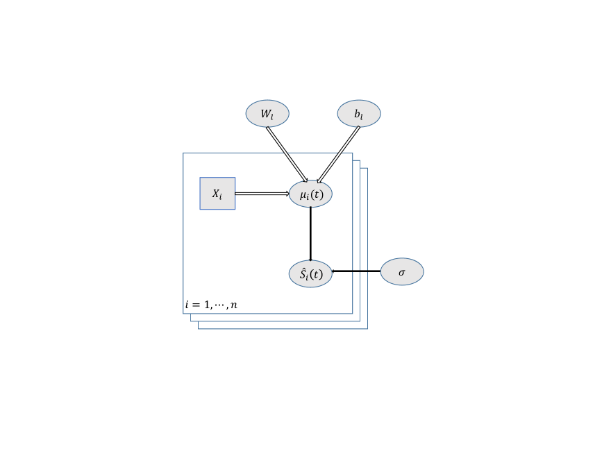
In the Bayesian hierarchical DNN model, the survival probability at each time , , follows a normal distribution:
| (2) |
The mean of the normal distribution, , is the transformation of covariates to a desired target value , and the variance of the normal distribution is . For prior distributions of parameters of affine transformation in , we assumed: the components of , , follow a normal distribution
| (3) |
and the components of , , follow a normal distribution
| (4) |
Furthermore, we assumed follows a uniform distribution . A directed acyclic graph (DAG) representation of the BDNNSurv model was shown in Figure 2.
The setup of the BDNNSurv, including the likelihood function in equation (2) and priors in equations (3) and (4), is standard in Bayesian hierarchical models. However, the automated Markov chain Monte Carlo (MCMC) approach can fail due to the lack of conjugate priors and high-dimensional parameter space in DNN.
A faster alternative to the MCMC is to use the variational inference (VI) (wainwright2008), which has been successfully applied in many large-scale problems (hoffman2013; blei2017). The VI turns the problem of computing a posterior distribution into an optimization problem. The traditional VI algorithm requires tedious model-specific derivations and implementation, which hindered its wide usage. Recently an automate process of deriving scalable VI algorithms, the so-called automatic differentiation variational inference (ADVI), has been developed in probabilistic programming (kucukelbir2017). The ADVI automatically develops an algorithm given a model, enabling an efficiently computation of Monte Carlo approximations. For more details on the ADVI, see kucukelbir2017 and references therein.
To implement the BDNNSurv, we adopted the same architecture, the good performance of which was demonstrated in zhao2019. There are three layers in the DNN with , and . The activation functions and are hyperbolic tangent functions and is sigmoid function. For the prior distributions of and , we let and for every layer and every component of and . In addition, we assign an uniform prior as the prior distribution of standard deviation of . Based on the posterior distributions of and , we obtain the posterior distributions of pseudo survival probabilities.
To adopt the ADVI, we used PyMC3 (salvatier2016), an open source probabilistic programming framework written in Python that builds on Theano (theano2016) with ADVI implementation. The initial values of and were obtained from running the DNN model proposed in zhao2019. The Python code implementing the proposed approach was included in the Supplementary Material.
KM estimates used in creating the pseudo values are subject to covariate-dependent censoring bias. In this case, we propose to use the inverse of probability of censoring weighted (IPCW) estimator for the survival function, denoted by , which has been successful at reducing the bias (Binder:2014; Xiang:2012; zhao2019; zhao2020). We replace by in (1) to compute the IPCW pseudo conditional survival probabilities by
| (5) |
where and is the IPCW Nelson-Aalen estimator for the the cumulative hazard function and is estimated by
| (6) |
where is the observable counting process for subject is the at risk process for subject , and is the inverse of probability of censoring for subject at time . By assigning different weights for subjects based on their covariate values, is approximately unbiased if the censoring distribution is correctly specified (Binder:2014).
To accurately model the censoring times as a function of covariates, we followed the method in zhao2020. The random survival forest (RSF) proposed in ishwaran2008 was first applied to the full data to estimate the probability of censoring for each subject at each observed event time to compute in (6), and then these estimates were re-used in computing pseudo observations, which is the same as the idea of re-using censoring regression coefficients from the full data analysis in the leave-one-out estimator in Binder:2014. We denote this method as BDNNSurv-IPCW hereafter.
3 Simulation
We conducted a simulation study to evaluate the performance of the newly proposed BDNNSurv approach. Besides the BDNNSurv, we adopted another approach based on the Bayesian Additive Regression Trees (BART) method in chipman2010 and compared the results from two approaches. BART is a flexible Bayesian non-linear regression approach and has been demonstrated to be competitive with widely used machine learning models. BART is formulated in a Bayesian hierarchical modeling framework, and as such provides both predictions and prediction interval estimates for a variety of quantities of interest. The original BART was extended to handle survival data using discrete-time survival analysis (sparapani2016). Given the distinct event and censoring times: , where is the th order statistic among distinct observation times, the binary outcome of a subject with/without an event/censoring until time is modeled using package BART (rbart) in R. We used the default setup in the package except for the thinning parameter and coarsen times. We used thinning by a factor of 1 instead of 10 due to low computational speed of the BART as detailed in Section 5. To overcome memory overflow, we used coarsen times per the quantiles .
In addition to BART, we compared the BDNNSurv with another Bayesian non-parametric, non-proportional hazards survival model proposed in de2009, where an unconstrained model for survival regression was constructed based on the covariate-dependent Dirichlet process (DDP). The dependence across random distributions was modeled in an ANOVA-type fashion. We implemented the ANOVA DDP approach using package spBayesSurv (rddp) in R with the same parameters as specified in the example of the package.
Survival times were simulated from a Cox proportional hazards model with baseline hazard from log-logistic function using the inverse cumulative distribution function method (bender2005). First, a variable was generated from a uniform(0, 1) distribution. Second, ten continuous covariates: , were independently generated from standard normal distributions; one binary covariate was generated from a Bernoulli distribution with probability taking 1 equal to 0.5. Let . Finally, the survival time was equal to:
| (7) |
where
| (8) |
, , and . To simulate survival times, we introduced a non-linear function with interaction into the hazard function through . Furthermore, we simulated the covariates and as noise variables. The noise variables were not used to generate survival times. However, they were included in the model.
In addition to survival times, the censoring times were independently generated from an exponential distribution. A rate parameter was chosen to obtain a censoring rate of about 20%. Survival times greater than 15 were censored at 15.
We generated one hundred data sets with each having 5000 subjects. Of the 5000 subjects, 75% were randomly selected as training data and the remaining 25% as test data. We estimated parameters using the training data and then predicted the survival probabilities along with corresponding 95% credible intervals on the test data from the to quantile of the survival function, with an increment of 10%. Note that the credible interval was used to quantify the uncertainty of survival probability. There is 95% probability that a given credible interval contains the true value of corresponding survival probability.
To demonstrate the performance of BDNNSurv, we investigated the cases with different sample sizes, censoring rates, numbers of predictor variables, and magnitude of parameter in matrix of equation (8). Furthermore, we simulated data from a non-proportional hazards (non-PH) model. Finally, we considered the case of covariate-dependent censoring. See Table 1 for different simulation setups.
To simulate data from a non-PH model, we let , where follows a Bernoulli distribution with the probability parameter being equal to 0.5. In the covariate-dependent censoring case, the censoring distribution was the same as the survival time distribution, except that we adjusted parameter to achieve 40% censoring rate.
| Case | Model | Number of Covariates X | in | Censoring Rate | |
|---|---|---|---|---|---|
| 1 | PH | 5000 | 10 | 0.5 | 20% |
| 2 | PH | 5000 | 10 | 0.5 | 40% |
| 3 | PH | 2000 | 10 | 0.5 | 20% |
| 4 | PH | 5000 | 10 | 0.95 | 20% |
| 5 | PH | 5000 | 50 | 0.5 | 20% |
| 6 | Non-PH | 5000 | 10 | 0.5 | 20% |
| 7 | PH IPCW | 5000 | 10 | 0.5 | 40% |
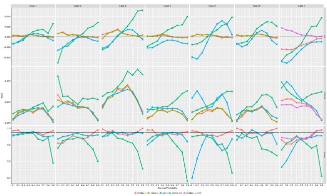
To compare different methods, we evaluated the statistical properties of both point and corresponding uncertainty estimates. For point estimates, we compared the bias and square root of mean squared error (MSE) of the estimated survival probabilities at different time points. The best model should have the smallest bias and MSE. The coverage probabilities were calculated for 95% credible intervals. The best model should have the coverage cloest to the nominal value 95%. We compared our BDNNSurv to BART and ANOVA DDP. We also compared with DNNSurv (zhao2019), regarding the bias and squared MSE (DNNSurv does not provide estimate of uncertainty). In case 7, we also compared with the BDNNSurv-IPCW.
The simulation results of case 1 and 5-7 are shown in Figure 3 and results of cases 2-4 are provided in Supplementary Material. For the point estimates, the BDNNSurv and DNNSurv had very similar results. In general, the BDNNSurv outperformed BART and ANOVA DDP, as evidenced by smaller bias, comparable MSE, and coverage probability closer to the nominal value. BART seems to perform the worst in most scenarios. ANOVA DDP didn’t perform well when the number of noise variables is large (case 5), and when the covariate-dependent censoring is present (case 7). As expected, the BDNNSurv-IPCW outperformed the other methods, when the covariate-dependent censoring is present, because other methods can only handle independent censoring.
4 Real Data
We applied the BDNNSurv approach to the Cardiovascular Health Study (CHS) data. CHS is a prospective, multicenter cohort study for coronary heart disease and stroke. The study is sponsored by the National Heart Lung and Blood Institute of the National Institutes of Health.
The study was initiated in 1987 to determine the risk factors for development and progression of cardiovascular disease (CVD) in older adults, with an emphasis on subclinical measures. The event of interest was time to CVD. The study has collected a large number of variables at baseline, including demographics (e.g., age, gender and race), family history of CVD, lab results, and medication information, with the goal to identity important risk factors for the CVD event. Detailed description of the study can be found in DrPhilos1993.
We selected 29 predictor variables after excluding the ones with more than 20% missing values. Furthermore, after excluding subjects with missing data in any of the selected predictor variables, we chose subjects, 65.2% of which had CVD during the study period. We randomly selected 75% subjects as training data and the other 25% as test data.
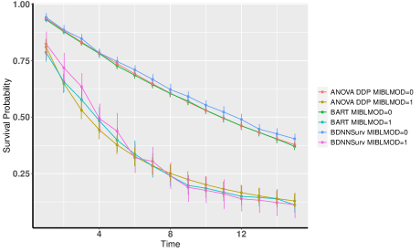
After building the BDNNSurv model using training data, we predicted the survival probability of subjects in the test data in every year up to 15 years. Figure 4 shows the survival functions for subjects with certain predictor variables, including myocardial infarction, chronic liver diseases, and stroke status, which are known to be important risk factors for the CVD event. The apparent separation of 95% confidence intervals of survival curves across time points demonstrated that subjects without risk factor (level 0) had significantly larger (at the significance level of 0.05) survival rates as compared to that with risk factor (level 1).
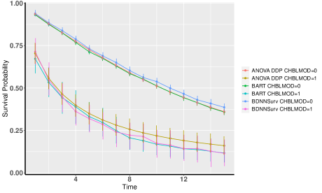
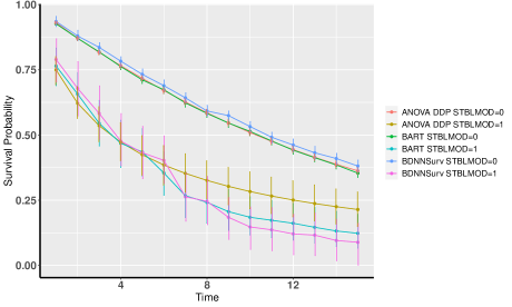
In the CHS data analysis, to obtain the estimate of survival probabilities at 15 different time points (year 1 to year 15 with an increment of 1 year), our BDNNSurv method is faster compared to the BART and ANOVA DDP. It took about 7, 20, and 185 minutes for BDNNSurv, ANOVA DDP, and BART, respectively, to run 10,000 iterations on an Intel(R) Core(TM) i7-4790 CPU 3.6 GHz, 32 GB RAM computer.
5 Concluding Remarks
Modeling and prediction of TTE data with high-dimensional covariates has recently drawn a lot of attention. Different DNN-based approaches have been studied. The previously proposed methods, however, can only provide point estimate without quantification of the corresponding uncertainty, which can be of crucial importance in predictive modeling and subsequent decision making. In this study, we proposed the BDNNSurv, a Bayesian hierarchical deep neural networks model, for modeling and prediction of TTE data. Our proposed model accurately predicted the survival probability along with the corresponding uncertainty, as demonstrated by simulation studies and real data analysis.
We specified the prior distributions based on the online documentation of PyMC3 (salvatier2016). For the prior distributions of and , we assumed and . We started with and and also tried or 2. For the prior distribution of , we tried , , and . We decided to use and , which produced estimates with good performance, including smaller bias, MSE, and coverage probabilities closer to the nominal value in case 1 of the simulation study. The choice of prior distributions is important in Bayesian neural networks and can have a large influence on the final results (silvestro2020). We suggest treating these hyper-parameters in the prior distributions as tuning parameters in the data analysis.
In future work, we will extend the proposed framework to accommodate complex biological information, such as gene-expression data, in survival prediction using different architectures e.g. convolutional neural networks (lopez2020). Moreover, we adopted variational inference to estimate posterior survival probabilities. Instead, in principle, one can compute an approximation to the posterior distribution by sampling multiple predictions with dropout. The dropout approach can also quantify uncertainty in deep learning (gal2016). In the future, it would be interesting to compare the results from two different methods.
Supplementary Material
The code used for simulation, including R code to simulate data and summarize results, python code to generate initial values for BDNNSurv, python code to run BDNNSurv, and R code to run BART and ANOVA DDP.
Acknowledgments
This Manuscript was prepared using the CHS data obtained from the National Heart, Lung, and Blood Institute (NHLBI) Biologic Specimen and Data Repository Information Coordinating Center (https://biolincc.nhlbi.nih.gov/), and does not necessarily reflect the opinions or views of the NHLBI.
References
- Andersen and Klein (2007) Andersen PK, Klein JP (2007). Regression analysis for multistate models based on a pseudo-value approach, with applications to bone marrow transplantation studies. Scandinavian Journal of Statistics, 34(1): 3–16.
- Andersen et al. (2003) Andersen PK, Klein JP, Rosthøj S (2003). Generalised linear models for correlated pseudo-observations, with applications to multistate models. Biometrika, 90: 15–27.
- Andersen and Perme (2010) Andersen PK, Perme MP (2010). Pseudo-observations in survival analysis. Statistical Methods in Medical Research, 19: 71–99.
- Bender et al. (2005) Bender R, Augustin T, Blettner M (2005). Generating survival times to simulate cox proportional hazards models. Statistics in Medicine, 24(11): 1713–1723.
- Binder et al. (2014) Binder N, Gerds TA, Andersen PK (2014). Pseudo-observations for competing risks with covariate dependent censoring. Lifetime Data Analysis, 20: 303–315.
- Blei et al. (2017) Blei DM, Kucukelbir A, McAuliffe JD (2017). Variational inference: A review for statisticians. Journal of the American Statistical Association, 112(518): 859–877.
- Ching et al. (2018) Ching T, Zhu X, Garmire LX (2018). Cox-nnet: An artificial neural network method for prognosis prediction of high-throughput omics data. PLoS Computational Biology, 14: e100607.
- Chipman et al. (2010) Chipman HA, George EI, McCulloch RE (2010). BART: Bayesian additive regression trees. The Annals of Applied Statistics, 4(1): 266–298.
- De Iorio et al. (2009) De Iorio M, Johnson WO, Müller P, Rosner GL (2009). Bayesian nonparametric nonproportional hazards survival modeling. Biometrics, 65(3): 762–771.
- Fotso (2018) Fotso S (2018). Deep neural networks for survival analysis based on a multi-task framework. arXiv preprint arXiv:1801.05512.
- Gal and Ghahramani (2016) Gal Y, Ghahramani Z (2016). Dropout as a bayesian approximation: Representing model uncertainty in deep learning. In: International Conference on Machine Learning, 1050–1059.
- Gensheimer and Narasimhan (2019) Gensheimer MF, Narasimhan B (2019). A scalable discrete-time survival model for neural networks. PeerJ, 7: e6257.
- Ghahramani (2015) Ghahramani Z (2015). Probabilistic machine learning and artificial intelligence. Nature, 521(7553): 452–459.
- Giunchiglia et al. (2018) Giunchiglia E, Nemchenko A, van der Schaar M (2018). RNN-SURV: A deep recurrent model for survival analysis. International Conference on Artificial Neural Networks, 90: 15–27.
- Hoffman et al. (2013) Hoffman MD, Blei DM, Wang C, Paisley J (2013). Stochastic variational inference. The Journal of Machine Learning Research, 14(1): 1303–1347.
- Ishwaran et al. (2008) Ishwaran H, Kogalur UB, Blackstone EH, Lauer MS (2008). Random survival forests. Annals of Applied Statistics, 2(3): 841–860.
- Katzman et al. (2018) Katzman JL, Shaham U, Cloninger A, Bates J, Jiang T, Kluger Y (2018). Deepsurv: personalized treatment recommender system using a cox proportional hazards deep neural network. BMC Medical Research Methodology, 18(1): 1–12.
- Kendall and Gal (2017) Kendall A, Gal Y (2017). What uncertainties do we need in Bayesian deep learning for computer vision? In: Advances in Neural Information Processing Systems, 5574–5584.
- Klein and Andersen (2005) Klein JP, Andersen PK (2005). Regression modeling of competing risks data based on pseudovalues of the cumulative incidence function. Biometrics, 61(1): 223–229.
- Kucukelbir et al. (2017) Kucukelbir A, Tran D, Ranganath R, Gelman A, Blei DM (2017). Automatic differentiation variational inference. The Journal of Machine Learning Research, 18(1): 430–474.
- Lee et al. (2018) Lee C, Zame W, Yoon J, van der Schaar M (2018). Deephit: A deep learning approach to survival analysis with competing risks. In: Proceedings of the AAAI Conference on Artificial Intelligence, volume 32.
- Leibig et al. (2017) Leibig C, Allken V, Ayhan MS, Berens P, Wahl S (2017). Leveraging uncertainty information from deep neural networks for disease detection. Scientific Reports, 7(1): 17816.
- López-García et al. (2020) López-García G, Jerez JM, Franco L, Veredas FJ (2020). Transfer learning with convolutional neural networks for cancer survival prediction using gene-expression data. PLoS One, 15(3): e0230536.
- Luck et al. (2017) Luck M, Sylvain T, Cardinal H, Lodi A, Bengio Y (2017). Deep learning for patient-specific kidney graft survival analysis. arXiv preprint arXiv:1705.10245.
- Martinsson (2016) Martinsson E (2016). WTTE-RNN: Weibull time to event recurrent neural network. Master’s thesis, University of Gothenburg, Sweden.
- Nielsen (2015) Nielsen MA (2015). Neural networks and deep learning, volume 25. Determination Press San Francisco, CA.
- Salvatier et al. (2016) Salvatier J, Wiecki TV, Fonnesbeck C (2016). Probabilistic programming in python using pymc3. PeerJ Computer Science, 2: e55.
- Silvestro and Andermann (2020) Silvestro D, Andermann T (2020). Prior choice affects ability of bayesian neural networks to identify unknowns. arXiv preprint arXiv:2005.04987.
- Sparapani et al. (2021) Sparapani R, Spanbauer C, McCulloch R (2021). Nonparametric machine learning and efficient computation with Bayesian additive regression trees: The BART R package. Journal of Statistical Software, 97(1): 1–66.
- Sparapani et al. (2016) Sparapani RA, Logan BR, McCulloch RE, Laud PW (2016). Nonparametric survival analysis using bayesian additive regression trees (BART). Statistics in Medicine, 35(16): 2741–2753.
- Tayob and Murray (2017) Tayob N, Murray S (2017). Statistical consequences of a successful lung allocation system–recovering information and reducing bias in models for urgency. Statistics in medicine, 36(15): 2435–2451.
- Tell et al. (1993) Tell GS, Fried LP, Hermanson B, Manolio TA, Newman AB, Borhani NO (1993). Recruitment of adults 65 years and older as participants in the cardiovascular health study. Annals of Epidemiology, 3(4): 358–366.
- Theano Development Team (2016) Theano Development Team (2016). Theano: A Python framework for fast computation of mathematical expressions. arXiv e-prints, abs/1605.02688.
- Wager et al. (2014) Wager S, Hastie T, Efron B (2014). Confidence intervals for random forests: The jackknife and the infinitesimal jackknife. The Journal of Machine Learning Research, 15(1): 1625–1651.
- Wainwright and Jordan (2008) Wainwright MJ, Jordan MI (2008). Graphical models, exponential families, and variational inference. Now Publishers Inc.
- Xiang and Murray (2012) Xiang F, Murray S (2012). Restricted mean models for transplant benefit and urgency. Statistics in Medicine, 6: 561–76.
- Zhao (2020) Zhao L (2020). Deep neural networks for predicting restricted mean survival times. Bioinformatics, 36(24): 5672–5677.
- Zhao and Feng (2020) Zhao L, Feng D (2020). Deep neural networks for survival analysis using pseudo values. IEEE Journal of Biomedical and Health Informatics, 24(11): 3308–3314.
- Zhao et al. (2020) Zhao L, Murray S, Mariani LH, Ju W (2020). Incorporating longitudinal biomarkers for dynamic risk prediction in the era of big data: A pseudo-observation approach. Statistics in Medicine, 39: 3685–3699.
- Zhou et al. (2020) Zhou H, Hanson T, Zhang J (2020). spBayesSurv: Fitting Bayesian spatial survival models using R. Journal of Statistical Software, 92(9): 1–33.
- Zhu et al. (2016) Zhu X, Yao J, Huang J (2016). Deep convolutional neural network for survival analysis with pathological images. In: 2016 IEEE International Conference on Bioinformatics and Biomedicine (BIBM), 544–547.