Fast imaging of multimode transverse-spectral correlations for twin photons

Abstract

Hyperentangled photonic states – exhibiting nonclassical correlations in several degrees of freedom – offer improved performance of quantum optical communication and computation schemes. Experimentally, a hyperentanglement of transverse-wavevector and spectral modes can be obtained in a straightforward way with multimode parametric single-photon sources. Nevertheless, experimental characterization of such states remains challenging. Not only single-photon detection with high spatial resolution – a single-photon camera – is required, but also a suitable mode-converter to observe the spectral/temporal degree of freedom. We experimentally demonstrate a measurement of a full 4-dimensional transverse-wavevector–spectral correlations between pairs of photons produced in the non-collinear spontaneous parametric downconversion (SPDC). Utilization of a custom ultra-fast single-photon camera provides high resolution and a short measurement time.

Photonic qubits can be easily created in entangled states, communicated over many–km distances and efficiently measured (Gisin and Thew, 2007). Tremendous effort has been devoted to improving the success rates of quantum enhanced protocols and multimode solutions, often accompanied with active multiplexing, are one of the most promising branches of this development (Collins et al., 2007; Parniak et al., 2017; Mazelanik et al., 2019; Lipka et al., 2020, 2019; Wen et al., 2019; Tian et al., 2017; Hiemstra et al., 2020; Pu et al., 2017; Kaneda and Kwiat, 2019), enabling both faster transfer and generation of photonic quantum states. In particular, systems harnessing several degrees of freedom (DoF) offer superior performance (Yang et al., 2018; Graffitti et al., 2020; Brecht et al., 2015) especially in selected protocols such as superdense coding (Barreiro et al., 2008), quantum teleportation (Wang et al., 2015) or complete Bell-state analysis (Walborn et al., 2003). Utilization of several DoFs brings a qualitatively new possibility to create hyperentangled states exhibiting nonclassical correlations in several DoF simultaneously with a greatly expanded Hilbert space and informational capacity. Generation of entangled pairs of photons in spectral, temporal, transverse wavevector, spatial, orbital angular momentum (OAM) and with multiple DoFs has been demonstrated. In particular spontaneous parametric down-conversion (SPDC) can be used to generate hyperentangled states in 4 DoF simultaneously (Barreiro et al., 2005). Nonetheless, experimental characterization of multidimensional states remains challenging. Single-pixel detectors such as superconducting nanowires offer excellent timing resolution Caloz et al. (2018), as well as spectral resolution when combined with dispersive elements such as chirped fiber gratings (Davis et al., 2017) or detector-integrated diffraction gratings Cheng et al. (2019). Such setups provide a way to implement high-dimensional quantum communication (Zhong et al., 2015), temporal super-resolved imaging Donohue et al. (2018) or observe quantum-interference in time or frequency space Jin et al. (2015); Jachura et al. (2018) - a promising approach for quantum fingerprinting (Jachura et al., 2017; Lipka et al., 2020). Single-photon-resolving cameras on the other hand naturally offer spatial or angular resolution, which can be exploited in super-resolution imaging (Tenne et al., 2019; Moreau et al., 2019; Mikhalychev et al., 2019; Schwartz et al., 2013; Parniak et al., 2018), interferometry Jachura et al. (2016), characterization (Defienne and Gigan, 2019; Reichert et al., 2018) or, similarly as in the previous case, observation of quantum interference effects such as in the Hong-Ou-Mandel–type experiments (Devaux et al., 2020). Recently however, the capability of cameras has been expanded by invoking a well-known mode conversion technique, in which Sun et al. simply observed spectral correlation with the help of a diffraction grating (Sun et al., 2019). It is thus a promising approach to use a camera to observe many DoFs simultaneously.

Here, we experimentally demonstrate a measurement of full 4-dimensional correlations between the transverse and spectral degrees of freedom of a twin-photon state, generated in a non-collinear type I SPDC. An ultra-fast single-photon–sensitive camera, yielding $10^{4}$ frames per second with $100\times 1952$ pixels per frame, allows to quickly gather enormous statistic size while maintaining high resolution due to a large number of pixels. In conjunction with recent development in high-dimensional entanglement detection (Bavaresco et al., 2018), our single-photon detection system would enable rapid characterization of such hyperentangled states. Furthermore, precise correlation measurements are vital to fully utilize quantum advantage of entangled states e.g. via non-local dispersion compensation recently demonstrated to improve quantum key distribution rates (Neumann et al., 2020). Higher-order correlation measurements also enable novel super-resolution imaging techniques (Mikhalychev et al., 2019; Moreau et al., 2019) which particularly benefit from fast acquisition rates and high spatial resolution of employed single-photon detectors.

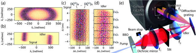
Figure 1: (a) Annular ring of twin-photon emission in the far-field of a BBO crystal mediating non-collinear type-I SPDC. Histogram of single photon positions has been registered over $2\times 10^{5}$ camera frames. (b) Twin-photon emission in the far-field after passing through the rectangular slit selecting $k_{y}\approx 0$ and after diffraction on the grating acting as wavelength-dependent wavevector shift $k_{y}\rightarrow k_{y}+K_{\text{grating}}(\lambda)$. Distinct fragments correspond to signal and idler photons, respectively. Camera frame coordinates correspond to transverse wavevectors and wavelength of photons. (c),(d) Camera regions corresponding to (c) signal and (d) idler photons. The division into sub-regions with limited wavevectors $\{k_{x}^{(s)}\},\{k_{x}^{(i)}\}$ and wavelengths $\{\lambda_{s}\},\{\lambda_{i}\}$ has been depicted with rectangles. For clarity only wavevector sub-regions (c) or only wavelength sub-regions (d) has been shown. Signal and idler regions are divided equally. (e) Experimental setup for fast transverse-spectral correlation imaging of twin-photons.

The employed camera prototype is an order of magnitude frame rate improvement over the off-the-shelf devices, necessary for a direct high-resolution measurement of 4-dimensional correlations. Prior approaches involved scaning the wavevector space with point detectors and used time-of-flight spectrometers for the spectral resolution, applicable at the telecom wavelengths and requiring compressed sensing techniques (Montaut et al., 2018). We note that a measurement in two mutually unbiased bases characterizes entanglement of pure bipartite, high-dimensional states without a state tomography (Bavaresco et al., 2018). In this context, our method would require extension to a position/time measurement basis to fully measure quantum correlations.

To generate twin-photon states we have employed a Beta Barium Borate (BBO) non-linear crystal in the type I SPDC process with noncollinear geometry, as depicted in Fig. 1. For the SPDC pumping we first produce second harmonic of $70\;\text{fs}$, $800\;\text{nm}$ pulses from Ti-Sapphire laser (Spectra Physics Mai Tai, 80 MHz repetition rate) in a second, similar BBO crystal with length $L=0.5\;\text{mm}$. The $800\;\text{nm}$ red pump is filtered-out with dichroic mirrors and a bandpass filter ($400\;\text{nm}$, $10\;\text{nm}$ bandwidth). Blue $\lambda_{p}=400\;\text{nm}$ pump with an average power of $70\;\text{mW}$ is focused in an $L=2\;\text{mm}$ BBO with a Gaussian beam width of $w_{0}=70\;\mu\text{m}$ and finally filtered-out with a dichroic mirror. The SPDC emission is far-field imaged with a lens ($f_{1}=60\;\text{mm}$) on an adjustable rectangular slit which selects a range of wavevectors $[-\Delta k_{y}/2,\Delta k_{y}/2]$ around $k_{y}=0$. A second lens ($f_{2}=300\;\text{mm}$) images the BBO onto a ruled diffraction grating ($N_{\text{lines}}=1200\;\text{lines/mm}$, resolution of $\delta\lambda=2\lambda_{p}/N_{\text{lines}}=0.66\;\text{nm}$) mounted vertically in the Littrow configuration and at a small horizontal angle. The grating adds a wavelength-dependent wavevector in the $y$ direction. A third lens ($f_{3}=100\;\text{mm})$ far-field images the grating onto a single-photon camera. The effective focal size of the setup from BBO to the camera is $f_{\text{eff}}=30\;\text{mm}$. A finite slit width $\Delta k_{y}$ corresponds to a resolution comparable to that of the diffraction grating $\delta\lambda$ when the image of the slit and a spectral point of $\delta\lambda$ size are compared in the camera image.

While BBO is cut for type I SPDC, by slightly adjusting the angle of the crystal axis with respect to the pump beam, we can alter the diameter and width of the far-field annular SPDC emission ring. Comparing with theory, the crystal-axis–$z$-axis angle (including cutting $29.2^{\circ}$) is $31.95^{\circ}\pm 0.025^{\circ}$. We estimate the overall efficiency of our at ca. $4\%$ roughly corresponding to the twin-photon generation ($50\%$), diffraction grating ($50\%$) and detection ($20\%$) efficiencies combined.

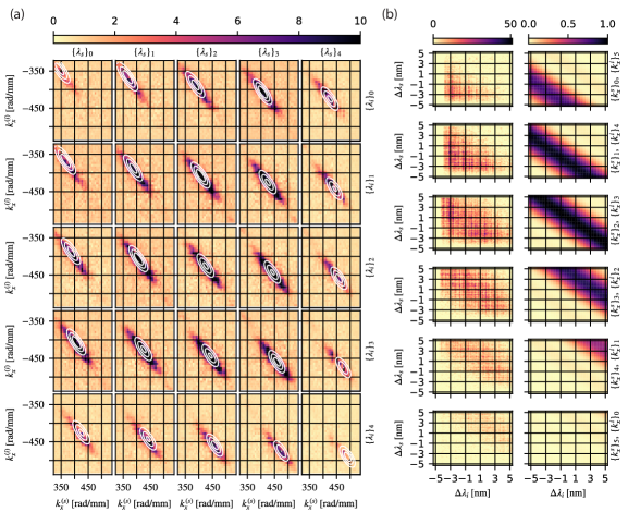
Figure 2: Correlation in joint (a) transverse wavevectors and (b) spectrum of signal–idler photon pairs. (a) Color map or (b) left column represents the experimental data (photon number covariance summed over (a) spectral or (b) wavevector regions, see main text). (a) White contours or (b) right column represents theoretical prediction $\scriptstyle|\Psi_{\{\lambda_{s}\},\{\lambda_{i}\}}(k_{x}^{(s)},k_{x}^{(i)})|^{2}$ of a two-photon wavefunction modulus squared, (a) summed over spectral ranges $\scriptstyle\{\lambda_{s}\},\{\lambda_{i}\}$ or (b) transverse-wavevector ranges $\scriptstyle\{k_{x}^{(s)}\},\{k_{x}^{(i)}\}$ and normalized to a unity maximum.

The single-photon camera consists of a two-stage image intensifier (Hamamatsu V7090-D) with high-voltage supply (Photek FP630) and a $10\;\text{kHz}$ gating module (Photek GM10-50B) connected with a custom-built I-sCMOS camera based on a fast CMOS sensor (LUX2100, pixel pitch $10\;\mu\text{m}$). Communication with the camera sensor and low-level image processing are performed with a programmable logic (FPGA) module (Xilinx Zynq-7020). The image processing consists of background subtraction and single-photon localization. FPGA module is bundled with an ARM-family processor, providing Ethernet data transfer to PC. The CMOS sensor is set for lowest time-dependent noise at the cost of lower dynamic range. With a faster gating module the camera could operate at $10^{5}$ frames per second with a frame of $10\times 1952$ px. Single-photon sensitivity is achieved by operating the image intensifier (II) in the Geiger mode (on/off) (Lipka et al., 2018) (see supplementary material - SM).

The gating time was $1.2\;\mu\text{s}$ with an average of $\bar{n}_{tot}=0.12$ photons per frame. Signal and idler photons are observed in $40\times 70\;\text{px}$ regions each corresponding to $416\;\text{rad/mm}\times 5.1\;\text{nm}$ (with $5.95\;\text{rad}/(\text{mm}\times\text{px})$ and $0.127\;\text{nm}/\text{px}$). The Gaussian mode size $\sigma_{k\text{-mode}}$ was predicted to be $6.2\;\text{rad/mm}$ and measured as $7.1\pm 0.3\;\text{rad}/\text{mm}$. The spectral mode size was measured to be $\sigma_{\lambda\text{-mode}}=4.20\pm 0.06\;\text{nm}$. We define the mode sizes as the Gaussian widths of a two-dimensional second-order photon number correlation in the sum coordinates $(k_{x}^{(s)}+k_{x}^{(i)},\lambda_{s}+\lambda_{i})$ (see SM). Using the theoretical prediction of the joint wavefunction we numerically get $M=1/\sum_{j=0}^{\infty}\lambda_{j}^{2}\approx 4.7$ accessible entangled modes, where $\lambda_{j}$ are the Schmidt coefficients (see SM). Note that for our considerations regarding the mode size and the number of modes we implicitly assumed a Gaussian two-photon wavefunction (leading to Gaussian second-order correlations) and as well as purity of the generated state.

While with a spectrally broad, focused pump beam and a short crystal, the SPDC emission is highly multimode in the spectral and transverse DoF, we begin with a single pair of signal ($s$)– idler ($i$) modes. A two-mode squeezed state $|\psi\rangle=\sum_{j=0}\chi^{j/2}|j\rangle_{s}|j\rangle_{i}$, generated in SPDC can be approximated to the first order in $\sqrt{\chi}$ as a pair of photons $|1\rangle_{s}|1\rangle_{i}$. Consider the joint wavefunction in transverse-wavevector and spectral coordinates:

$$\Psi(\bm{k}_{s,\perp},\lambda_{s};\bm{k}_{i,\perp},\lambda_{i})=\langle\bm{k}_{s,\perp},\lambda_{s}|1\rangle_{s}\langle\bm{k}_{i,\perp},\lambda_{i}|1\rangle_{i}.$$ (1)

We directly measure the $x$ component of the transverse wavevector, while selecting photons with $k_{y}\approx 0$. Before measurement, a diffraction grating maps the spectral DoF onto $k_{y}(\omega)$. Single-photon camera detects the number of photons with a given transverse–spectral coordinate $n(k_{x}^{(\xi)},\lambda_{\xi})\in\{0,1\};\;\xi\in\{s,i\}$ separately in signal and idler arms. With a large number of observed frames, the average over frames $\scriptstyle\langle n(k_{x}^{(\xi)},\lambda_{\xi})\rangle$ gives an estimate for the probability of detecting a photon at given coordinates. Hence, the photon number covariance:

$$\mathcal{C}(k_{x}^{(s)},\lambda_{s};\;k_{x}^{(i)},\lambda_{i})=\\ \langle n(k_{x}^{(s)},\lambda_{s})n(k_{x}^{(i)},\lambda_{i})\rangle-\langle n(k_{x}^{(s)},\lambda_{s})\rangle\langle n(k_{x}^{(i)},\lambda_{i})\rangle$$ (2)

estimates the probability of detecting a non-accidental coincidence – pair of correlated signal and idler photons in a single camera frame – with given spectral and transverse coordinates, modeled by $|\Psi(\bm{k}_{s,\perp},\lambda_{s};\bm{k}_{i,\perp},\lambda_{i})|^{2}$. The camera gating time encompasses ca. 96 pump laser repetitions, hence 96 temporal modes are aggregated in each camera frame, producing accidental coincidences between photons from different temporal modes. The second term in Eq. (2) roughly corresponds to these accidental coincidences. For visualization, we sum the covariance over selected sub-regions either in wavelengths $\{\lambda_{s}\},\{\lambda_{i}\}$ or wavevectors $\{k_{x}^{(s)}\},\{k_{x}^{(i)}\}$ yielding:

$$\mathcal{C}_{\{\lambda_{s}\},\{\lambda_{i}\}}(k_{x}^{(s)},k_{x}^{(i)}) =\smashoperator[lr]{\sum_{\begin{subarray}{c}\lambda_{s}\in\{\lambda_{s}\},\lambda_{i}\in\{\lambda_{i}\}\end{subarray}}^{}}\mathcal{C}(k_{x}^{(s)},\lambda_{s};\;k_{x}^{(i)},\lambda_{i}),$$ (3)

$$\mathcal{C}_{\{k_{x}^{(s)}\},\{k_{x}^{(i)}\}}(\lambda_{s},\lambda_{i}) =\smashoperator[lr]{\sum_{\begin{subarray}{c}k_{x}^{(s)}\in\{k_{x}^{(s)}\},k_{x}^{(i)}\in\{k_{x}^{(i)}\}\end{subarray}}^{}}\mathcal{C}(k_{x}^{(s)},\lambda_{s};\;k_{x}^{(i)},\lambda_{i}).$$ (4)

The selected sub-regions are depicted in Fig. 1 (c),(d) on a histogram of signal and idler positions in wavevector–wavelength space. During the measurement we gathered $10^{9}$ camera frames, each serving as a separate experiment repetition. The joint covariance in transverse wavevector coordinates $\mathcal{C}_{\{\lambda_{s}\},\{\lambda_{i}\}}(k_{x}^{(s)},k_{x}^{(i)})$ is depicted in Fig. 2 (a) with each panel corresponding to a different pair of wavelength sub-regions $\{\lambda_{s}\},\{\lambda_{i}\}$. Good agreement with the theoretical prediction can be observed with only the crystal-axis–z-axis angle fitted (a small deviation from the cutting angle). The details of wavefunction calculation can be found in Supplementary Material. Similarly, the joint covariance in spectral coordinates $\mathcal{C}_{\{k_{x}^{(s)}\},\{k_{x}^{(i)}\}}(\lambda_{s},\lambda_{i})$ is depicted in Fig. 2 (b) for selected pairs of sub-regions in which the covariance is non-vanishing. selecting $k_{y}\approx 0$ limits observations of the 6-dimensional space of two-photon transverse-spectral correlations to a 4-dimensional slice. The limitation can be relevant for complex transverse correlations e.g. from a biaxial crystal.

We have demonstrated a capability to measure 4 dimensional transverse-wavevector–spectral correlations between pairs of photons generated in non-collinear SPDC. Due to a custom single-photon camera with very fast acquisition rates (an order of magnitude improvement) we were able to gather statistics of $10^{9}$ camera frames (experiment repetitions) in roughly one day. Large statistics enabled faithful reconstruction of bi-photon wavevefunction in spectral and transverse-wavevector coordinates. For this demonstration we selected a single component of the transverse wavevector which is far-field imaged (mapped) onto positions on the camera frame, similarly the spectral part is mapped onto positions with a diffraction grating. Importantly, our system is inherently multimode and can be adapted for measurements in different mode bases e.g. orbital angular momentum and for different degrees of freedom.

Funding

Ministry of Science and Higher Education (DI2018 010848); Foundation for Polish Science (MAB/2018/4 “Quantum Optical Technologies”); Office of Naval Research (N62909-19-1-2127).

Disclosures

The authors declare no conflicts of interest.

Supplementary Material

Bi-photon amplitude and photon number covariance

Let us begin with the positive part of the blue pump classical electric field:

$$E_{p}^{(+)}(\bm{r},t)=\\ \mathcal{E}_{p}\int\mathrm{d}^{2}\bm{k}_{p,\perp}\mathrm{d}\omega_{p}A_{p}(\bm{k}_{p,\perp},\omega_{p})\exp[i(\bm{k}_{p}\cdot\bm{r}-\omega_{p}t)],$$ (5)

where $\mathcal{E}_{p}$ denotes the pump pulse amplitude, $\bm{k}_{p,\perp}$ its transverse wavevector and $A_{p}$ corresponds to the normalized slowly varying envelope of the pulse. From the wavefunction of the state generated in SPDC we shall consider only the biphoton part (Kolenderski et al., 2009), which can be denoted as:

$$|\Psi\rangle=\int\mathrm{d}^{2}\bm{k}_{s,\perp}\mathrm{d}^{2}\bm{k}_{i,\perp}\mathrm{d}\omega_{s}\mathrm{d}\omega_{i}\Psi(\bm{k}_{s,\perp},\omega_{s};\bm{k}_{i,\perp},\omega_{i})\times\\ \hat{a}^{\dagger}(\bm{k}_{s,\perp},\omega_{s})\hat{a}^{\dagger}(\bm{k_{i,\perp}},\omega_{i})|\text{vac}\rangle,$$ (6)

where $s,i$ indices correspond to signal and idler photons, respectively. For a crystal with length $L$ and assuming the $z$ axis points along the pump beam’s central wavevector, the biphoton amplitude $\Psi(\bm{k}_{s,\perp},\omega_{s};\bm{k}_{i,\perp},\omega_{i})$ is given by:

$$\Psi(\bm{k}_{s,\perp},\omega_{s};\bm{k}_{i,\perp},\omega_{i})=\mathcal{N}\int_{-L/2}^{L/2}\mathrm{d}z\>\big{\{}\\ A_{p}(\bm{k}_{s,\perp}+\bm{k}_{i,\perp},\omega_{s}+\omega_{i})\exp[i\Delta k_{z}(\bm{k}_{s,\perp},\omega_{s};\bm{k}_{i,\perp},\omega_{i})z]\big{\}},$$ (7)

where the phase mismatch $\Delta k_{z}(\bm{k}_{s,\perp},\omega_{s};\bm{k}_{i,\perp},\omega_{i})$ is determined by the $z$ components of the wavevectors:

$$\Delta k_{z}(\bm{k}_{s,\perp},\omega_{s};\bm{k}_{i,\perp},\omega_{i})=k_{p,z}(\bm{k}_{s,\perp}+\bm{k}_{i,\perp},\omega_{s}+\omega_{i})-\\ k_{s,z}(\bm{k}_{s,\perp},\omega_{s})-k_{i,z}(\bm{k}_{i,\perp},\omega_{i}).$$ (8)

Note that we work in the paraxial approximation. In particular since $|\bm{k}_{\perp}|\ll|\bm{k}|$ and the crystal’s index of refraction changes slowly over the range of observed wavevectors, we can assume that the transverse wavevector components within and outside the crystal are equal (at the crystal-air boundary the emission angle increases by a factor equal to the crystal’s index of refraction but so does the total wavevector, hence the transverse component must remain unchanged in the small-angle approximation).

Integrating Eq. (8) along $z$ we get:

$$\Psi(\bm{k}_{s,\perp},\omega_{s};\bm{k}_{i,\perp},\omega_{i})=\\ \mathcal{N}A_{p}(\bm{k}_{s,\perp}+\bm{k}_{i,\perp},\omega_{s}+\omega_{i})\text{sinc}[\frac{L\Delta k_{z}(\bm{k}_{s,\perp},\omega_{s};\bm{k}_{i,\perp},\omega_{i})}{2}].$$ (9)

In our experiment we select a narrow range of $k_{y}$ around $k_{y}=0$. Hence, we shall simplify the notation $\mathbf{k_{\alpha,\perp}}\rightarrow k_{x}^{(\alpha)};\;\alpha\in\{s,i\}$. Importantly, $|\Psi(k_{x}^{(s)},\omega_{s};\;k_{x}^{(i)},\omega_{i})|^{2}$ is proportional to the probability of simultaneously generating a signal photon with transverse wavevector $k_{x}^{(s)}$ and wavelength $\lambda_{s}=2\pi c/\omega_{s}$ and an idler photon with $k_{x}^{(i)}$ and $\lambda_{i}=2\pi c/\omega_{i}$. Clearly, if the bi-photon term vanishes $|\Psi(k_{x}^{(s)},\omega_{s};\;k_{x}^{(i)},\omega_{i})|^{2}=0$ for some coordinates $(k_{x}^{(s)},\omega_{s},k_{x}^{(i)},\omega_{i})$, the probability of observing a photon pair in $(k_{x}^{(s)},\omega_{s},k_{x}^{(i)},\omega_{i})$ is equal to the product of marginal probabilities of observing a signal photon at $(k_{x}^{(s)},\omega_{s})$ and of observing an idler photon at $(k_{x}^{(i)},\omega_{i})$. Hence, $|\Psi(k_{x}^{(s)},\omega_{s};\;k_{x}^{(i)},\omega_{i})|^{2}$ is proportional to photon number covariance between signal and idler modes $\mathcal{C}(k_{x}^{(s)},\lambda_{s};\;k_{x}^{(i)},\lambda_{i})$.

For direct comparison with measured covariances we sum the modulus squared amplitudes in the selected wavelength and wavevectors regions, respectively:

$$|\Psi_{\{\lambda_{s}\},\{\lambda_{i}\}}(k_{x}^{(s)},k_{s}^{(i)})|^{2}=\\ \sum_{\lambda_{s}\in\{\lambda_{s}\},\lambda_{i}\in\{\lambda_{i}\}}|\Psi(k_{x}^{(s)},2\pi c/\lambda_{s};\;k_{x}^{(i)},2\pi c/\lambda_{i})|^{2},$$ (10)

$$|\Psi_{\{k_{x}^{(s)}\},\{k_{x}^{(i)}\}}(\lambda_{s},\lambda_{i})|^{2}=\\ \sum_{k_{x}^{(s)}\in\{k_{x}^{(s)}\},k_{x}^{(i)}\in\{k_{x}^{(i)}\}}|\Psi(k_{x}^{(s)},2\pi c/\lambda_{s};\;k_{x}^{(i)},2\pi c/\lambda_{i})|^{2}.$$ (11)

Non-classical correlations and mode size

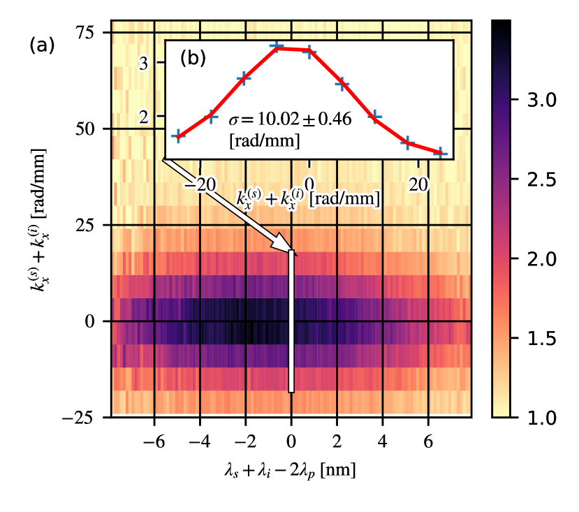
Figure 3: (a) Second order photon number correlation function $g^{(2)}(k_{x}^{(s)}+k_{x}^{(i)},\lambda_{i}+\lambda_{s})$ between signal and idler photons, in sum coordinates of spectral and temporal DoF. (b) Cross section for $\lambda_{i}+\lambda_{s}=2\lambda_{p}$. Data (blue crosses) is depicted against a Gaussian fit (red solid) with Gaussian width parameter $\sigma=10.02\pm 0.46\;[\text{rad/mm}]$.

To quantify the non-classical character of signal–idler correlations and estimate the mode size we employ the second-order photon number correlation function defined for a single pair of signal–idler modes as:

$$g^{(2)}(k_{x}^{(s)},\lambda_{s};\;k_{x}^{(i)},\lambda_{i})=\frac{\langle n(k_{x}^{(s)},\lambda_{s})n(k_{x}^{(i)},\lambda_{i})\rangle}{\langle n(k_{x}^{(s)},\lambda_{s})\rangle\langle n(k_{x}^{(i)},\lambda_{i})\rangle}.$$ (12)

For visualization we sum the coincidences and the normalizing factor over the uncorrelated directions to get:

$$g^{(2)}(k_{+},\lambda_{+})=\\ \sum_{k_{-},\lambda_{-}}\langle n(k_{x}^{(s)},\lambda_{s})n(k_{x}^{(i)},\lambda_{i})\rangle(k_{+},k_{-};\;\lambda_{+},\lambda_{-})/\\ \big{\{}\sum_{k_{-},\lambda_{-}}\langle n(k_{x}^{(s)},\lambda_{s})\rangle(k_{+},k_{-};\;\lambda_{+},\lambda_{-})\\ \times\langle n(k_{x}^{(i)},\lambda_{i})\rangle(k_{+},k_{-};\;\lambda_{+},\lambda_{-})\big{\}}$$ (13)

with $k_{\pm}=k_{x}^{(s)}\pm k_{i}^{(i)}$, $\lambda_{\pm}=\lambda_{s}\pm\lambda_{i}$ and where we implicitly transformed the mean photon numbers to $\pm$ coordinates. As depicted in Fig. 3, the cross-section for degenerate wavelength $\lambda_{i}+\lambda_{s}=2\lambda_{p}$ has a Gaussian shape with width $\sigma=10.02\pm 0.46\;[\text{rad/mm}]$. This width corresponds to the the transverse wavevector mode size of SPDC emission as

$$\sigma_{k\text{-mode}}=\frac{\sigma}{\sqrt{2}},$$ (14)

where the $\sqrt{2}$ factor comes from the Jacobian of $(k_{x}^{(s)},k_{x}^{(i)})\rightarrow(k_{x}^{(s)}+k_{x}^{(i)},k_{x}^{(s)}-k_{x}^{(i)})$ transformation. Similarly, the Gaussian fit for $k_{x}^{(s)}=-k_{x}^{(i)}$ cross-section gives $\sigma_{\lambda\text{-mode}}=4.20\pm 0.06\;\text{nm}$. If we trace over the idler (signal) mode, the remaining signal (idler) has a thermal photon count statistics with autocorrelation $g_{\text{idler,auto}}^{(2)}=g_{\text{signal,auto}}^{(2)}=g_{\text{therm,auto}}^{(2)}\leq 2$; hence, according to Cauchy–Schwarz inequality the upper classical bound on the second order cross-correlation function is $g_{\text{classical}}^{(2)}\leq\sqrt{g_{\text{signal,auto}}^{(2)}g_{\text{idler,auto}}^{(2)}}=2$.

Schmidt number

We estimate the number of modes by considering the theoretical prediction for the biphoton wavefunction, given by Eq. (9). We numerically compute the wavefunction in a range of experimentally observed wavelengths and transverse wavevectors. The obtained tensor is reshaped into a two dimensional matrix with a single dimension corresponding to the spectral and transverse coordinates of a single photon. Singular value decomposition of the resulting matrix yields the Schmidt coefficients $\{\lambda_{j}\}$. The Schmidt number (defined as per ref. (Zielnicki et al., 2018)) is given by:

$$M=(\sum_{j=0}^{\infty}\lambda_{j}^{2})^{-1}\approx 4.7,$$ (15)

and corresponds to the approximate number of accessible entangled modes.

Single-photon sensitivity of the custom CMOS camera

The image intensifier (II) is operated in the Geiger mode (on/off). A photon striking the II leads to the emission of a photoelectron (with quantum efficiency of $20\%)$ which is accelerated ($-200\;\text{V}$) or stopped ($+50\;\text{V}$) with an electric potential controlled by the gating module. The accelerated photoelectrons are multiplied via avalanche secondary emission in a two-stage microchannel plate (MCP) giving $10^{6}$ output electrons per photoelectron. The voltage across MCP is $1800\;\text{V}$. Electrons leaving the MCP are further accelerated ($6000\;\text{V}$) and strike a phosphor (P46) screen, leaving bright flashes. The phosphor screen is imaged (magnification $M=0.44)$ with a relay lens onto the CMOS sensor. We note that while we cross-correlate two regions for signal and idler photons, respectively, an auto-correlation setup could be employed with a single region and simple post-processing (Lipka et al., 2018).

Setup efficiency

We estimate the efficiency using a reference free method. Assuming a noiseless case, a single spatial mode and $R$ temporal modes per camera frame we have $\langle n_{x}\rangle=R\eta\chi,\;x\in\{i,s\}$, $\langle n_{i}n_{s}\rangle=R\eta^{2}\chi+\langle n_{i}\rangle\langle n_{s}\rangle$, where $\eta$ is the overall efficiency. Hence,

$$\eta=\frac{\langle n_{i}n_{s}\rangle-\langle n_{i}\rangle\langle n_{s}\rangle}{\sqrt{\langle n_{i}\rangle\langle n_{s}\rangle}}=\frac{g^{(2)}-1}{\sqrt{\langle n_{i}\rangle\langle n_{s}\rangle}}.$$ (16)

Using $g^{(2)}=\max_{\lambda_{+},k_{+}}[g^{(2)}(\lambda_{+},k_{+})]$ and global average numbers of photons $\langle n_{i}\rangle$, $\langle n_{s}\rangle$ we get $\eta\approx 4\%$.

References

- Gisin and Thew (2007) N. Gisin and R. Thew, Nature Photonics 1, 165 (2007).
- Collins et al. (2007) O. A. Collins, S. D. Jenkins, A. Kuzmich, and T. A. B. Kennedy, Phys. Rev. Lett. 98, 060502 (2007).
- Parniak et al. (2017) M. Parniak, M. Dąbrowski, M. Mazelanik, A. Leszczyński, M. Lipka, and W. Wasilewski, Nat. Commun. 8, 2140 (2017).
- Mazelanik et al. (2019) M. Mazelanik, M. Parniak, A. Leszczyński, M. Lipka, and W. Wasilewski, npj Quantum Inf. 5, 22 (2019).
- Lipka et al. (2020) M. Lipka, M. Mazelanik, and M. Parniak, “Entanglement distribution with wavevector-multiplexed quantum memory,” arXiv:2007.00538 (2020).
- Lipka et al. (2019) M. Lipka, A. Leszczyński, M. Mazelanik, M. Parniak, and W. Wasilewski, Phys. Rev. Appl. 11, 034049 (2019).
- Wen et al. (2019) Y. Wen, P. Zhou, Z. Xu, L. Yuan, H. Zhang, S. Wang, L. Tian, S. Li, and H. Wang, Phys. Rev. A 100, 012342 (2019).
- Tian et al. (2017) L. Tian, Z. Xu, L. Chen, W. Ge, H. Yuan, Y. Wen, S. Wang, S. Li, and H. Wang, Phys. Rev. Lett. 119, 130505 (2017).
- Hiemstra et al. (2020) T. Hiemstra, T. Parker, P. Humphreys, J. Tiedau, M. Beck, M. Karpiński, B. Smith, A. Eckstein, W. Kolthammer, and I. Walmsley, Phys. Rev. Applied 14, 014052 (2020).
- Pu et al. (2017) Y. F. Pu, N. Jiang, W. Chang, H. X. Yang, C. Li, and L. M. Duan, Nat. Commun. 8, 15359 (2017).
- Kaneda and Kwiat (2019) F. Kaneda and P. G. Kwiat, Science Advances 5, 10 (2019).
- Yang et al. (2018) T.-S. Yang, Z.-Q. Zhou, Y.-L. Hua, X. Liu, Z.-F. Li, P.-Y. Li, Y. Ma, C. Liu, P.-J. Liang, X. Li, Y.-X. Xiao, J. Hu, C.-F. Li, and G.-C. Guo, Nat. Commun. 9, 3407 (2018).
- Graffitti et al. (2020) F. Graffitti, V. D’Ambrosio, M. Proietti, J. Ho, B. Piccirillo, C. d. Lisio, L. Marrucci, and A. Fedrizzi, “Hyperentanglement in structured quantum light,” arXiv:2006.01845 (2020).
- Brecht et al. (2015) B. Brecht, D. V. Reddy, C. Silberhorn, and M. G. Raymer, Phys. Rev. X 5, 041017 (2015).
- Barreiro et al. (2008) J. T. Barreiro, T.-C. Wei, and P. G. Kwiat, Nature Physics 4, 282 (2008).
- Wang et al. (2015) X.-L. Wang, X.-D. Cai, Z.-E. Su, M.-C. Chen, D. Wu, L. Li, N.-L. Liu, C.-Y. Lu, and J.-W. Pan, Nature 518, 516 (2015).
- Walborn et al. (2003) S. P. Walborn, S. Pádua, and C. H. Monken, Phys. Rev. A 68, 042313 (2003).
- Barreiro et al. (2005) J. T. Barreiro, N. K. Langford, N. A. Peters, and P. G. Kwiat, Phys. Rev. Lett. 95, 260501 (2005).
- Caloz et al. (2018) M. Caloz, M. Perrenoud, C. Autebert, B. Korzh, M. Weiss, C. Schönenberger, R. J. Warburton, H. Zbinden, and F. Bussières, Applied Physics Letters 112, 061103 (2018), https://doi.org/10.1063/1.5010102 .
- Davis et al. (2017) A. O. C. Davis, P. M. Saulnier, M. Karpiński, and B. J. Smith, Opt. Express 25, 12804 (2017).
- Cheng et al. (2019) R. Cheng, C.-L. Zou, X. Guo, S. Wang, X. Han, and H. X. Tang, Nature Communications 10, 4104 (2019).
- Zhong et al. (2015) T. Zhong, H. Zhou, R. D. Horansky, C. Lee, V. B. Verma, A. E. Lita, A. Restelli, J. C. Bienfang, R. P. Mirin, T. Gerrits, S. W. Nam, F. Marsili, M. D. Shaw, Z. Zhang, L. Wang, D. Englund, G. W. Wornell, J. H. Shapiro, and F. N. C. Wong, New Journal of Physics 17, 022002 (2015).
- Donohue et al. (2018) J. M. Donohue, V. Ansari, J. Řeháček, Z. Hradil, B. Stoklasa, M. Paúr, L. L. Sánchez-Soto, and C. Silberhorn, Phys. Rev. Lett. 121, 090501 (2018).
- Jin et al. (2015) R.-B. Jin, T. Gerrits, M. Fujiwara, R. Wakabayashi, T. Yamashita, S. Miki, H. Terai, R. Shimizu, M. Takeoka, and M. Sasaki, Opt. Express 23, 28836 (2015).
- Jachura et al. (2018) M. Jachura, M. Jarzyna, M. Lipka, W. Wasilewski, and K. Banaszek, Phys. Rev. Lett. 120, 110502 (2018).
- Jachura et al. (2017) M. Jachura, M. Lipka, M. Jarzyna, and K. Banaszek, Opt. Express 25, 27475 (2017).
- Lipka et al. (2020) M. Lipka, M. Jarzyna, and K. Banaszek, IEEE Journal on Selected Areas in Communications 38, 496 (2020).
- Tenne et al. (2019) R. Tenne, U. Rossman, B. Rephael, Y. Israel, A. Krupinski-Ptaszek, R. Lapkiewicz, Y. Silberberg, and D. Oron, Nature Photonics 13, 116 (2019).
- Moreau et al. (2019) P.-A. Moreau, E. Toninelli, T. Gregory, and M. J. Padgett, Nature Reviews Physics 1, 367 (2019).
- Mikhalychev et al. (2019) A. B. Mikhalychev, B. Bessire, I. L. Karuseichyk, A. A. Sakovich, M. Unternährer, D. A. Lyakhov, D. L. Michels, A. Stefanov, and D. Mogilevtsev, Communications Physics 2, 134 (2019).
- Schwartz et al. (2013) O. Schwartz, J. M. Levitt, R. Tenne, S. Itzhakov, Z. Deutsch, and D. Oron, Nano Letters 13, 5832 (2013).
- Parniak et al. (2018) M. Parniak, S. Borówka, K. Boroszko, W. Wasilewski, K. Banaszek, and R. Demkowicz-Dobrzański, Phys. Rev. Lett. 121, 250503 (2018).
- Jachura et al. (2016) M. Jachura, R. Chrapkiewicz, R. Demkowicz-Dobrzański, W. Wasilewski, and K. Banaszek, Nature Communications 7, 11411 (2016).
- Defienne and Gigan (2019) H. Defienne and S. Gigan, Phys. Rev. A 99, 053831 (2019).
- Reichert et al. (2018) M. Reichert, H. Defienne, and J. W. Fleischer, Scientific Reports 8, 7925 (2018).
- Devaux et al. (2020) F. Devaux, A. Mosset, P.-A. Moreau, and E. Lantz, Phys. Rev. X 10, 031031 (2020).
- Sun et al. (2019) K. Sun, J. Gao, M.-M. Cao, Z.-Q. Jiao, Y. Liu, Z.-M. Li, E. Poem, A. Eckstein, R.-J. Ren, X.-L. Pang, H. Tang, I. A. Walmsley, and X.-M. Jin, Optica 6, 244 (2019).
- Bavaresco et al. (2018) J. Bavaresco, N. Herrera Valencia, C. Klöckl, M. Pivoluska, P. Erker, N. Friis, M. Malik, and M. Huber, Nature Physics 14, 1032 (2018).
- Neumann et al. (2020) S. P. Neumann, D. Ribezzo, M. Bohmann, and R. Ursin, “Experimentally optimizing qkd rates via nonlocaldispersion compensation,” arXiv:2007.00362v2 (2020).
- Montaut et al. (2018) N. Montaut, O. S. Magaña-Loaiza, T. J. Bartley, V. B. Verma, S. W. Nam, R. P. Mirin, C. Silberhorn, and T. Gerrits, Optica 5, 1418 (2018).
- Lipka et al. (2018) M. Lipka, M. Parniak, and W. Wasilewski, Appl. Phys. Lett. 112, 211105 (2018).
- Kolenderski et al. (2009) P. Kolenderski, W. Wasilewski, and K. Banaszek, Phys. Rev. A 80, 013811 (2009).
- Zielnicki et al. (2018) K. Zielnicki, K. Garay-Palmett, D. Cruz-Delgado, H. Cruz-Ramirez, M. F. O’Boyle, B. Fang, V. O. Lorenz, A. B. U’Ren, and P. G. Kwiat, Journal of Modern Optics 65, 1141 (2018).