Extrapolating the thermodynamic length with finite-time measurements

Abstract

The excess work performed in a heat-engine process with given finite operation time $\tau$ is bounded by the thermodynamic length, which measures the distance during the relaxation along a path in the space of the thermodynamic state. Unfortunately, the thermodynamic length, as a guidance for the heat engine optimization, is beyond the experimental measurement. We propose to measure the thermodynamic length $\mathcal{L}$ through the extrapolation of finite-time measurements $\mathcal{L}(\tau)=\int_{0}^{\tau}[P_{\mathrm{ex}}(t)]^{1/2}dt$ via the excess power $P_{\mathrm{ex}}(t)$. The current proposal allows to measure the thermodynamic length for a single control parameter without requiring extra effort to find the optimal control scheme. We illustrate the measurement strategy via examples of the quantum harmonic oscillator with tuning frequency and the classical ideal gas with changing volume.

Introduction.—Optimization of thermodynamic processes is of practical importance in finite-time thermodynamics (Berry et al., 2000; de Koning, 2005; Schmiedl and Seifert, 2007; Andresen, 2011; Cavina et al., 2018a; Solon and Horowitz, 2018) to minimize the dissipation in finite-time transformation processes (Aurell et al., 2011, 2012; Zulkowski and DeWeese, 2014; Proesmans et al., 2020a, b), and to improve the performance of real heat engines (Curzon and Ahlborn, 1975; Esposito et al., 2010a, b; de Tomás et al., 2012; Cavina et al., 2018b; Abiuso and Perarnau-Llobet, 2020; Lee et al., 2020; Singh, 2020; Zhang, 2020a). The extent, to which the optimization can be achieved, is discovered to be limited by the geometry properties of the thermodynamic equilibrium state space (Weinhold, 1975; Ruppeiner, 1979; Gilmore, 1984; Salamon et al., 1985; Ruppeiner, 1995; Crooks, 2007; Feng and Crooks, 2009) and provides a criterion for the amelioration of specific control schemes. For a finite-time isothermal process with operation time $\tau$, such optimization is realized by minimizing the entropy production (Salamon et al., 1980; Diósi et al., 1996; Zulkowski and DeWeese, 2015a, b) or the excess work $W_{\mathrm{ex}}=W-\Delta F$ (Bonança and Deffner, 2014, 2018; Zhang, 2020b), where $W$ is the total performed work and $\Delta F$ is the free energy change. For a given control scheme, the excess work at the long-time limit is bounded as $W_{\mathrm{ex}}\geq\mathcal{L}^{2}/\tau$ (Salamon and Berry, 1983; Nulton et al., 1985; Tu, 2012; Gong et al., 2016; Cavina et al., 2017; Ma et al., 2018), where $\mathcal{L}$ is the thermodynamic length during the relaxation dynamics (Sivak and Crooks, 2012; Zulkowski et al., 2012; Rotskoff and Crooks, 2015; Sivak and Crooks, 2016). In the recent development of finite-time quantum thermodynamics (Esposito et al., 2009; Campisi et al., 2011; Kosloff, 2013; Vinjanampathy and Anders, 2016; Strasberg et al., 2017), the thermodynamic length relates to the geometric measures of quantum states, such as the Bures length and the Fisher or the Wigner-Yanase skew information (Deffner and Lutz, 2010, 2013; Mancino et al., 2018; Pires et al., 2016; Bengtsson, 2017), and provides a lower bound of the excess work and the entropy production in a finite-time quantum thermodynamic process (Scandi and Perarnau-Llobet, 2019; Brandner and Saito, 2020; Abiuso et al., 2020; Miller and Mehboudi, 2020).

However, it remains a challenge to practically measure the thermodynamics length in a real thermodynamic system. To obtain the metric of the state space, one needs the exact equilibrium thermal states along the path of the control parameters, which could be the frequency of harmonic oscillator or the volume of the classical ideal gas. One proposal for the measurement is the utilization of the discrete-step process (Crooks, 2007; Feng and Crooks, 2009), which requires significant amount of small steps. In this Letter, we define a finite-time thermodynamic length $\mathcal{L}(\tau),$ which retains the thermodynamic length at the long-time limit. The thermodynamic length $\mathcal{L}$ can be measured through extrapolating few data points of $\mathcal{L}(\tau)$ with finite duration $\tau$. The measurement procedure is illustrated via examples of the quantum harmonic oscillator with tuning frequency and the classical ideal gas with changing volume.

Finite-time thermodynamic length.—We consider an open quantum system with the control parameter $\lambda(t)$ tuned from the initial value $\lambda(0)=\lambda_{0}$ to the final value $\lambda(\tau)=\lambda_{\tau}$ in a finite-time process with duration $\tau$. The system state is described by the density matrix $\rho(t)$ $(0<t<\tau)$, which evolves under the time-dependent Hamiltonian $H(t)=H[\lambda(t)]$ via the time-dependent Markovian master equation (Albash et al., 2012; Yamaguchi et al., 2017; Dann et al., 2018)

$$\dot{\rho}=\mathscr{L}_{\lambda(t)}\rho,$$ (1)

where $\mathscr{L}_{\lambda(t)}$ is the quantum Liouvillian super-operator. In quantum thermodynamics, the rate of the performed work, namely the power, is $\dot{W}=\mathrm{Tr}(\rho\dot{H})$ (Alicki, 1979). In a quasi-static isothermal process with infinite duration, the system evolves along the trajectory of the equilibrium state $\rho_{\mathrm{eq}}(t)=\exp[-\beta_{\mathrm{b}}H(t)]/\mathrm{Tr\{}\exp[-\beta_{\mathrm{b}}H(t)]\}$ with the inverse temperature $\beta_{\mathrm{b}}=1/k_{\mathrm{B}}T_{\mathrm{b}}$ of the bath, and the performed work of the whole process is $W_{(0)}=\int_{\lambda_{0}}^{\lambda_{\tau}}\mathrm{\mathrm{Tr}}(\rho_{\mathrm{eq}}\partial H/\partial\lambda)d\lambda$. In a finite-time isothermal process, the excess work $W_{\mathrm{ex}}(\tau)=\int_{0}^{\tau}P_{\mathrm{ex}}(t)dt$ is utilized to evaluate the dissipation with the excess power (Sivak and Crooks, 2012) $P_{\mathrm{ex}}(t)=\dot{W}(t)-\dot{W}_{(0)}(t),$ where $\dot{W}_{(0)}(t)=\mathrm{\mathrm{Tr}}[\rho_{\mathrm{eq}}\dot{H}]$ is the quasi-static part of the work rate. One important progress (Sivak and Crooks, 2012; Zulkowski et al., 2012) for the finite-time thermodynamics is the discovery of the geometric bound of the excess work with the thermodynamic length as $W_{\mathrm{ex}}(\tau)\geq\mathcal{L}^{2}/\tau$, and the equality is saturated by the optimal protocol with the constant excess power. The direct measurement of thermodynamic length $\mathcal{L}$ requires the infinite slow isothermal processes (Crooks, 2007; Feng and Crooks, 2009).

In quantum thermodynamics, the thermodynamic length $\mathcal{L}$ is explicitly (Scandi and Perarnau-Llobet, 2019)

$$\mathcal{L}=\int_{\lambda_{0}}^{\lambda_{\tau}}\sqrt{\mathrm{\mathrm{Tr}}[\frac{\partial H}{\partial\lambda}\mathscr{L}_{\lambda}^{-1}(\frac{\partial\rho_{\mathrm{eq}}}{\partial\lambda})]}d\lambda,$$ (2)

which contains the Drazin inverse $\mathscr{L}_{\lambda}^{-1}$ of the super-operator (Mandal and Jarzynski, 2016; Crooks, 2018). For the diagonalizable super-operator, the Drazin inverse is explicitly obtained as follows. The eigendecomposition is $\mathscr{L}_{\lambda}=\sum_{\Gamma}\Gamma P_{\Gamma}$ with the eigenvalues $\Gamma$ and the projections $P_{\Gamma}$ in the super-space of the density matrices. The null eigenvector is the instantaneous equilibrium state satisfied $\mathscr{L}_{\lambda}[\rho_{\mathrm{eq}}(\lambda)]=0$. The Drazin inverse is then written as $\mathscr{L}_{\lambda}^{-1}=\sum_{\Gamma\neq 0}\Gamma^{-1}P_{\Gamma}$, where the inverses of the non-zero eigenvalues $\Gamma^{-1}$ determines different dissipation timescales (Mandal and Jarzynski, 2016; Crooks, 2018). Detailed discussions about the Drazin inverse are given with an example of the two-level system in the Supplementary Materials (sup, ).

For the measurement, we define a finite-time thermodynamic length as

$$\mathcal{L}(\tau)=\int_{0}^{\tau}\sqrt{P_{\mathrm{ex}}(t)}dt.$$ (3)

The two following properties of the finite-time thermodynamic length allows the measurement of the thermodynamics length with the extrapolation of finite-time measurements.

(i) The convergence $\underset{\tau\rightarrow\infty}{\lim}\mathcal{L}(\tau)=\mathcal{L}$. In a slow isothermal process, the state of the system evolves near the equilibrium state, and the solution to Eq. (1) is expanded in the series (Cavina et al., 2017) as

$$\rho(t)=\sum_{n=0}^{\infty}\left(\mathscr{L}_{\lambda(t)}^{-1}\frac{d}{dt}\right)^{n}\rho_{\mathrm{eq}}(t).$$ (4)

For a given tuning protocol $\lambda(t)=\tilde{\lambda}(t/\tau)$, the series expansion of the excess power is obtained as

$$P_{\mathrm{ex}}(t)=\mathrm{\mathrm{Tr}}\{\frac{\partial\tilde{H}(s)}{\partial s}\sum_{n=1}^{\infty}\tau^{1-n}(\mathscr{L}_{\tilde{\lambda}(s)}^{-1}\frac{\partial}{\partial s})^{n}[\tilde{\rho}_{\mathrm{eq}}(s)]\},$$ (5)

where $s=t/\tau$ is the rescaled dimensionless time. Equation (5) is invalid at the beginning of the isothermal process. Its validity requires a relaxation with the time larger than the typical dissipation timescale. For the slow process, the lowest-order term with $n=1$ dominates the summation, and the finite-time thermodynamic length approaches the thermodynamic length at the long-time limit.

(ii) The protocol independence of the limit $\underset{\tau\rightarrow\infty}{\lim}\mathcal{L}(\tau)$. For the system with only one control parameter, the limit of the finite-time thermodynamic length $\underset{\tau\rightarrow\infty}{\lim}\mathcal{L}(\tau)$ is independent of the protocol, which implies the thermodynamic length can be measured without necessarily using the optimal protocol. For multiple control parameters, the limit $\underset{\tau\rightarrow\infty}{\lim}\mathcal{L}(\tau)$ indeed relies on the path of the protocol. The minimal thermodynamic length is only reached by the geodesic path, and the optimized protocol is to tune the control parameter with the constant velocity of the thermodynamic length (Scandi and Perarnau-Llobet, 2019).

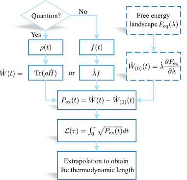
Figure 1: (Color online) Flowchart for measuring the thermodynamic length $\mathcal{L}$ with finite-time extrapolation. The excess power is evaluated with the performed work rate $\dot{W}(t)$ and the quasi-static work rate $\dot{W}_{(0)}(t)$ at each moment of the finite-time process.

Measurement strategy.—The thermodynamic length is the long-time limit of the finite-time thermodynamic length. In the following, we propose an extrapolation method to measure the thermodynamic length for the system with a single control parameter. The flowchart of the method is shown in Fig. 1. The measurement of the finite-time thermodynamic length $\mathcal{L}(\tau)$ requires the excess power $P_{\mathrm{ex}}(t)$ of the whole process. The power $\dot{W}(t)\;(0<t<\tau)$ in a finite-time process is measured through the conjugate force $f(t)=\mathrm{\mathrm{Tr}}[\rho\partial_{\lambda}H]$ for a classical system via $\dot{W}(t)=\dot{\lambda}(t)f(t)$ or the tomography of the density matrix $\rho(t)$ for a quantum system via $\dot{W}(t)=\mathrm{Tr}(\rho\dot{H})$. With the given protocol $\tilde{\lambda}(s)$ of the control parameter, the quasi-static work rate $\dot{W}_{(0)}(t)=\mathrm{Tr}(\rho_{\mathrm{eq}}\dot{H})=\dot{\lambda}\partial_{\lambda}F_{\mathrm{eq}}(\lambda)$ is obtained with the landscape of the equilibrium free energy $F_{\mathrm{eq}}(\lambda)$, which can be typically obtained from finite-time processes via Jarzynski’s equality (Jarzynski, 1997).

Assuming the length $\mathcal{L}(\tau)$ as a smooth function of the duration $\tau$, we expand $\mathcal{L}(\tau)$ with the Laurent series as

$$\mathcal{L}(\tau)=\mathcal{L}+\sum_{j=1}^{\infty}\frac{a_{j}}{\tau^{j}}.$$ (6)

The duration $\tau$ needs to be chosen notably larger than the dissipation timescale to ensure the validity of Eq. (5). By measuring the finite-time thermodynamic length under given duration, we extrapolate the function as $\mathcal{L}(\tau)=\mathcal{L}+\sum_{j=1}^{N}a_{j}\tau^{-j}$ with the cutoff $N$. The thermodynamic length $\mathcal{L}$ is estimated with the extrapolation $\tau\rightarrow\infty$. We apply the current strategy to measure the thermodynamic length with two examples, i.e. the quantum harmonic oscillator and the classical ideal gas system.

Quantum harmonic oscillator with tuned frequency.—We consider the quantum Brownian motion with the Hamiltonian $H(t)=\hat{p}^{2}/(2m)+m\omega(t)^{2}\hat{x}^{2}/2$ in a tuned harmonic potential with the frequency $\omega(t)$ as the control parameter in the finite-time isothermal process. At the high temperature limit, the evolution of the reduced system is described by the Caldeira-Leggett master equation (Caldeira and Leggett, 1983; Breuer and Petruccione, 2007), i.e, $\partial_{t}\rho=\mathscr{L}_{\omega(t)}\rho$. The quantum Liouvillian super-operator is explicitly

$$\mathscr{L}_{\omega(t)}\rho=-i[H(t),\rho]-i\kappa[\hat{x},\{\hat{p},\rho\}]-\frac{2m\kappa}{\beta_{\mathrm{b}}}[\hat{x},[\hat{x},\rho]],$$ (7)

where the frequency-independent damping rate $\kappa$ is induced by the Ohmic spectral of the heat bath (Caldeira and Leggett, 1983; Breuer and Petruccione, 2007).

With the infinite dimension of the Hilbert space for a harmonic oscillator, it is difficult to solve the evolution of the density matrix by calculating the Drazin inverse of the super-operator directly. An alternative way is to solve the finite-time dynamics via a closed Lie algebra (Rezek and Kosloff, 2006; Lee et al., 2020) with the thermodynamic variables, the Hamiltonian $H(t)$, the Lagrange $L(t)=\hat{p}^{2}/(2m)-m\omega(t)^{2}\hat{x}^{2}/2$ and the correlation function $D(t)=\omega(t)(\hat{x}\hat{p}+\hat{p}\hat{x})/2$. The closed differential equations of the expectations of the thermodynamic variables $\left\langle H(t)\right\rangle=\mathrm{Tr}[\rho(t)H(t)]$, $\left\langle L(t)\right\rangle=\mathrm{Tr}[\rho(t)L(t)]$ and $\left\langle D(t)\right\rangle=\mathrm{Tr}[\rho(t)D(t)]$ are obtained from Eq. (7) as

$$\frac{d}{dt}\left(\begin{array}[]{c}\left\langle H\right\rangle\\ \left\langle L\right\rangle\\ \left\langle D\right\rangle\end{array}\right)=\left(\begin{array}[]{ccc}-2\kappa+\frac{\dot{\omega}}{\omega}&-2\kappa-\frac{\dot{\omega}}{\omega}&0\\ -2\kappa-\frac{\dot{\omega}}{\omega}&-2\kappa+\frac{\dot{\omega}}{\omega}&-2\omega\\ 0&2\omega&-2\kappa+\frac{\dot{\omega}}{\omega}\end{array}\right)\left(\begin{array}[]{c}\left\langle H\right\rangle\\ \left\langle L\right\rangle\\ \left\langle D\right\rangle\end{array}\right)+2\kappa k_{B}T_{\mathrm{b}}\left(\begin{array}[]{c}1\\ 1\\ 0\end{array}\right).$$ (8)

The derivation to Eqs. (8) is presented in the Supplementary Materials (sup, ).

The performed work rate of the tuned harmonic oscillator is $\dot{W}=\dot{\omega}/\omega\left(\left\langle H\right\rangle-\left\langle L\right\rangle\right)$. In a quasi-static isothermal process, the system evolves along the equilibrium states with the average internal energy $\left\langle H\right\rangle=k_{B}T_{\mathrm{b}}$ and the average Lagrange $\left\langle L\right\rangle=0$, and the quasi-static work rate is $\dot{W}_{(0)}(t)=k_{B}T_{\mathrm{b}}\dot{\omega}/\omega$. In a finite-time process, the finite-time thermodynamic length $\mathcal{L}(\tau)$ is explicitly

$$\mathcal{L}(\tau)=\int_{0}^{\tau}\left[\dot{\omega}/\omega\left(\left\langle H\right\rangle-\left\langle L\right\rangle-k_{B}T_{\mathrm{b}}\right)\right]^{1/2}dt.$$ (9)

The thermodynamic length of the tuned harmonic oscillator is obtained by Eq. (2) as

$$\mathcal{L} =\sqrt{\frac{k_{B}T_{\mathrm{b}}}{2\kappa}}\left|\left[\text{sinh}^{-1}(\frac{\omega}{2\kappa})-\sqrt{1+\frac{4\kappa^{2}}{\omega^{2}}}\right]\Big{|}_{\omega=\omega_{0}}^{\omega_{\tau}}\right|,$$ (10)

where $\omega_{0}$ and $\omega_{\tau}$ are the initial and final frequencies of the harmonic potential. The detailed derivation of the thermodynamic length is given in the Supplementary Materials (sup, ). The optimal protocol $\omega_{\mathrm{op}}(t)=\tilde{\omega}_{\mathrm{op}}(t/\tau)$ satisfies

$$\left(\frac{1}{2\kappa}+\frac{2\kappa}{\tilde{\omega}_{\mathrm{op}}^{2}}\right)^{1/2}\frac{1}{\tilde{\omega}_{\mathrm{op}}}\frac{d\tilde{\omega}_{\mathrm{op}}(s)}{ds}=\mathrm{const}.$$ (11)

For small damping rate $\kappa\ll\omega$, the thermodynamic length approximates $\mathcal{L}\approx\sqrt{k_{B}T_{\mathrm{b}}/(2\kappa)}\left|\ln\omega_{\tau}/\omega_{0}\right|$, and the optimal protocol is the exponential protocol $\tilde{\omega}_{\mathrm{op}}(s)=\omega_{0}\exp[s\ln(\omega_{\tau}/\omega_{0})]$. For the large damping rate $\omega\ll\kappa$, the thermodynamic length approximates $\mathcal{L}\approx\sqrt{2\kappa k_{B}T_{\mathrm{b}}}\left|(\omega_{\tau}-\omega_{0})/(\omega_{0}\omega_{\tau})\right|$, and the optimal protocol is the inverse protocol $\tilde{\omega}_{\mathrm{op}}(s)=\omega_{0}\omega_{\tau}/[(\omega_{0}-\omega_{\tau})s+\omega_{\tau}]$.

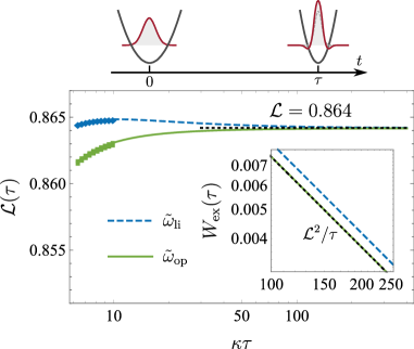
Figure 2: (Color online) Finite-time extrapolation to measure the thermodynamic length for the quantum Brownian motion in a tuned harmonic potential. The upper panel shows the frequency increases from $\omega_{0}=1$ to $\omega_{\tau}=2$. The temperature and the damping rate are set as $k_{B}T_{\mathrm{b}}=1$ and $\kappa=1$. In the lower panel, the black dotted line presents the thermodynamic length $\mathcal{L}=0.864$, which is approached by the extrapolated functions with $N=3$ for both the linear (blue dashed curve) and the optimal (green solid curve) protocols. The subset shows the excess work in a slow process is bounded as $W_{\mathrm{ex}}(\tau)\geq\mathcal{L}^{2}/\tau$ (black dotted line), which is saturated by the optimal protocol at the long-time limit.

We exemplify the finite-time extrapolation method to obtain the thermodynamic length of the tuned harmonic oscillator through numerically solving the relaxation dynamics with the linear protocol $\tilde{\omega}_{\mathrm{li}}(s)=\omega_{0}+(\omega_{\tau}-\omega_{0})s$ and the optimal protocol $\tilde{\omega}_{\mathrm{op}}(s)$. In the numerical calculation, the frequency is tuned from $\omega_{0}=1$ to $\omega_{\tau}=2$ with the temperature $k_{B}T_{\mathrm{b}}=1$ and the damping rate $\kappa=1$. In Fig. 2, the extrapolated functions (curves) with $N=3$ are obtained from 10 sets of data (markers) with the duration $\tau$ ranging from $6.4$ to $9.9$ for the linear (blue dashed line) and the optimal (the green solid line) protocols as $\mathcal{L}_{\mathrm{li}}(\tau)=0.864+0.0128/\tau-0.0464/\tau^{2}-0.145/\tau^{3}$ and $\mathcal{L}_{\mathrm{op}}(\tau)=0.864-0.00471/\tau-0.0448/\tau^{2}-0.168/\tau^{3}$. The two extrapolated functions both give the consistent thermodynamic length identical to the theoretical result $\mathcal{L}=0.864$ by Eq. (10), as illustrated with the dotted black line. Therefore the current extrapolation method enables the measurement of the thermodynamic length in relatively short time without the need to find the optimal protocol.

The subset shows the $\tau^{-1}$ scaling of the excess work. The black dotted line shows the bound $\mathcal{L}^{2}/\tau$, and the blue dashed (green solid) line shows the extra work with the linear (optimal) control scheme. The excess work of different protocols is indeed bounded by the thermodynamic length, and the bound is saturated by the optimal protocol.

Compression of classical ideal gas.— The extrapolation method is applicable in classical systems with the strategy shown in Fig. 1. We consider the finite-time compression of the classical ideal gas in a box, which is in contact with a heat bath at the temperature $T_{\mathrm{b}}$. By compressing the piston, the volume of the box changes with the performed work rate $\dot{W}=-p\dot{V}$. With the state equation $pV=nRT$, the temperature $T$ of the classical ideal gas satisfies

$$\frac{dT}{dt}=-\frac{nRT}{C_{V}}\frac{1}{V}\frac{dV}{dt}-\gamma(T-T_{\mathrm{b}}),$$ (12)

where $\gamma$ is the cooling rate in the Newton’s law of cooling, assumed as a constant in the following discussion, and $C_{V}$ is the heat capacity at the constant volume, e.g. $C_{V}=3nR/2$ for the single-atom ideal gas. In a finite-time isothermal process, the excess power is obtained as $P_{\mathrm{ex}}(t)=-nR(T-T_{\mathrm{b}})\dot{V}/V$. The thermodynamic length $\mathcal{L}$ is theoretically obtained as

$$\mathcal{L}=\sqrt{\frac{(nR)^{2}T_{\mathrm{b}}}{\gamma C_{V}}}\left|\ln\frac{V_{\tau}}{V_{0}}\right|.$$ (13)

For a long-time compression, the optimal protocol with the constant excess power is obtained as the exponential protocol $\tilde{V}_{\mathrm{op}}(s)=V_{0}(V_{\tau}/V_{0})^{s}$, which is consistent with the result obtained by the stochastic thermodynamics (Gong et al., 2016).

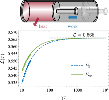
Figure 3: (Color online) Finite-time extrapolation to measure the thermodynamic length for the compression of the classical ideal gas in a box. The upper panel shows the compression of the box. In the lower panel, we use the linear protocol (blue dashed curve) and the optimal protocol (green solid curve) to compress the volume of the box to one half. With the current chosen parameters, the length extrapolated with the two protocols match the exact thermodynamic length $\mathcal{L}=0.566$ (black dotted line) by Eq. (13).

In Fig. 3, the finite-time thermodynamic lengths (markers) for given protocols are numerically obtained for the isothermal processes with the duration $\tau$ ranging from $11.0$ to $20.0$, where the parameters are set as $nR=T_{\mathrm{b}}=\gamma=1$ and $C_{V}=1.5$, and the volume is tuned from $V_{0}=1$ to $V_{\tau}=0.5$. Two protocols are considered to tune the volume linearly $\tilde{V}_{\mathrm{li}}(s)=1-s/2$ (blue dashed curve) and exponentially $\tilde{V}_{\mathrm{op}}(s)=2^{-s}$ (green solid curve). Setting the cutoff $N=3$, the extrapolated functions of the two protocols are $\mathcal{L}_{\mathrm{li}}(\tau)=0.566-0.318/\tau+0.010/\tau^{2}-0.146/\tau^{3}$ and $\mathcal{L}_{\mathrm{op}}(\tau)=0.566-0.216/\tau-0.199/\tau^{2}-0.111/\tau^{3}$. Both extrapolations with different protocols lead to the same value, matching the theoretical result $\mathcal{L}=0.566$ (black dotted line) given by Eq. (13).

Using examples of both the quantum harmonic oscillator and the classical ideal gas, we demonstrate the proposed extrapolation method for measuring the thermodynamic length for typical systems with single control parameter. The quantum harmonic oscillator system is potentially realized with the trapped ion (An et al., 2014; Rossnagel et al., 2016), and the classical ideal gas system will be tested with our recently designed apparatus (Ma et al., 2020).

Conclusion.—The thermodynamic length is crucial in optimization of finite-time isothermal processes, yet remains challenging to be practically measured in experiments. We have overcome the difficulty and proposed to measure the thermodynamic length via the finite-time extrapolation method, which allows to determine the lower bound of the excess work without necessarily using the optimal protocol. The protocol-independent property of the current measurement strategy benefits to practically measure the thermodynamic length in experiments. Based on our recent experimental setup (Ma et al., 2020), it is feasible to measure the thermodynamic length for the finite-time compression of the classical ideal gas in the experiments, which we leave as the goal for our future experimental research.