Radiative decay of the $\Xi(1620)$ in a hadronic molecule picture

Abstract

Last year, the $\Xi(1620)$ state that is cataloged in the Particle Data Group (PDG) with only one star is reported again in the $\Xi^{-}\pi^{+}$ final state by the Belle Collaboration. Its properties not only the spectroscopy but also the decay width cannot be simply explained in the context of conventional constituent quark models. This intrigues an active discussion on the structure of this resonance. In this work, we study the radiative decays of the newly observed $\Xi(1620)$ assuming that it is a meson-baryon molecular state of $\Lambda\bar{K}$ and $\Sigma\bar{K}$ with spin-parity $J^{P}=1/2^{-}$ in our previous work. The partial decay widths of the $\Lambda\bar{K}-\Sigma\bar{K}$ molecular state into $\Xi\gamma$ and $\Xi\pi\gamma$ final states through hadronic loops are evaluated with the help of the effective Lagrangians. The partial widths for the $\Xi(1620)^{0}\to\gamma\Xi$ and $\Xi(1620)^{0}\to\gamma\Xi\pi$ are evaluated to be about $118.76-174.21$ KeV and $58.19-68.75$ eV, respectively, which may be accessible for the LHCb. If the $\Xi(1620)$ is $\Lambda\bar{K}-\Sigma\bar{K}$ molecule, the radiative transition strength $\Xi(1620)^{0}\to\gamma\bar{K}\Lambda$ is quite small and the decay width is of the order of 0.01 eV. Future experimental measurements of these processes can be useful to test the molecule interpretations of the $\Xi(1620)$.

I INTRODUCTION

Searching for hadrons beyond the quark model becomes one of the most important topics in the community of hadron physics. In the conventional quark model, a hadron is composed of $q\bar{q}$ as a meson or $qqq$ as a baryon. It is natural to expect the existence of hadrons composed of more quarks, which are called exotic states. Due to the great experimental progress in the past 20 years, more and more exotic states have been observed Zyla:2020zbs . Last year, the $\Xi(1620)$ state that is cataloged in the Particle Data Group(PDG) Zyla:2020zbs with only one star is reported again in the $\Xi^{-}\pi^{+}$ final state by the Belle Collaboration Sumihama:2018moz . The observed resonance parameters of the structure are

$$M=1610.4\pm{6.0}(stat)^{+5.9}_{-3.5}(syst)~{}~{}{\rm MeV},$$

$$\Gamma=59.9\pm 4.8(stat)^{+2.8}_{-3.0}(syst)~{}~{}{\rm MeV},$$ (1)

which are consistent with the earlier measured values Ross:1972bf ; Briefel:1977bp . Its spin-parity, however, remains undetermined.

From the observed decay model, the $\Xi(1620)$ is a conventional baryon composed of $uss$ or $dss$. However, its properties not only the spectroscopy but also the decay width cannot be simply explained in the context of conventional constituent quark models Capstick:1986bm ; Blask:1990ez ; Azimov:2003bb . As indicated in Refs. Ramos:2002xh ; GarciaRecio:2003ks ; Gamermann:2011mq ; Miyahara:2016yyh ; Oh:2007cr ; Wang:2019krq ; Chen:2019uvv ; Huang:2020taj , the $\Xi(1620)$ can be understood as a molecular state in comparison with the Belle data Sumihama:2018moz . A molecular state with a narrow width and a mass around 1606 MeV was predicted in the unitarized coupled channels approach Ramos:2002xh ; GarciaRecio:2003ks ; Gamermann:2011mq ; Miyahara:2016yyh . However, a $\Xi$ bound state with a mass about 1620 MeV and $J^{P}=1/2^{-}$ is predicted by studying the $\bar{K}\Lambda$ interaction in the framework of the One-Boson-Exchange (OBE) model Chen:2019uvv . In other words, the Ref. Chen:2019uvv consider $\Xi(1620)$ as a pure molecular state composes of $\bar{K}\Lambda$ component. A possible explanation for these results of Refs. Ramos:2002xh ; GarciaRecio:2003ks ; Gamermann:2011mq ; Miyahara:2016yyh ; Chen:2019uvv is that the $\Xi$(1620) has a larger $\bar{K}\Lambda$ component Wang:2019krq ; Huang:2020taj . Moreover, the $\bar{K}\Sigma$ component can not be underestimated to reproduce the total decay width of the $\Xi(1620)$ and a study of the spectroscopy alone does not give a complete picture of its nature Huang:2020taj .

From the above discussion, the $\Xi(1620)$ may be a molecular state. However, at present, we cannot fully exclude other possible explanations such as a mixture of three quark and five quark components (as long as quantum numbers allow, it might well be the case). More efforts are necessary to distinguish whether it is a molecular state or a compact multi-quark state. The photon coupling with quark is really different from the coupling of the photon to the constituent $\bar{K}\Lambda$ and $\bar{K}\Sigma$ of the $\Xi(1620)$ Koniuk:1979vy . Hence, a precise measurement of the radiative decays is useful to test different interpretations of $\Xi(1620)$. In this work, we study the radiative decay of the $\Xi(1620)$ in the hadronic molecule approach developed in our previous study Huang:2020taj .

This paper is organized as follows. The theoretical formalism is explained in Sec.II. The predicted partial decay widths are presented in Sec.III, followed by a short summary in the last section.

II Theoretical FORMALISM

In our previous study Huang:2020taj , the total decay width of $\Xi(1620)$ can be reproduced with the assumption that the $\Xi(1620)$ is an $S-$wave $\bar{K}\Lambda-\bar{K}\Sigma$ bound state with $J^{P}=1/2^{-}$. According to the molecular scenario, the radiative decay widths $\Xi(1620)\to\gamma\Xi$, $\Xi(1620)\to\gamma\bar{K}\Lambda$ and, $\Xi(1620)\to\gamma\pi\Xi$ are studied to elucidate the internal structure of the $\Xi(1620)$. In order to calculate the radiation decay, we first employ the weinberg compositeness rule to determine $\Xi(1620)$ couplings to hers constituents $\bar{K}Y$ ($Y\equiv\Lambda,\Sigma$). The radiative decays then follow from the exchange of a suitable hadron between the $\bar{K}Y$ pair, which then transforms into $\Xi\gamma$,$\gamma\bar{K}\Lambda$, and $\Xi\pi\gamma$. The corresponding Feynman diagrams are shown in Fig. (1) and Fig. (2).

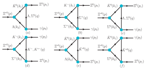
Figure 1: Feynman diagrams for the $\Xi^{*0}\to{}\gamma\Xi^{0}$ decay processes. We also show the definitions of the kinematics ($p,k_{1},k_{2},p_{1},p_{2}$, and $q$) used in the calculation.

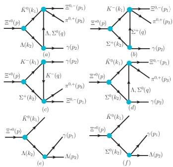
Figure 2: Feynman diagrams for the $\Xi^{*0}\to{}\gamma\Xi^{0}\pi^{0}$,$\gamma\Xi^{-}\pi^{+}$, and $\gamma\bar{K}\Lambda$ decay processes. We also show the definitions of the kinematics ($p,k_{1},k_{2},p_{1},p_{2}$,$p_{3}$, and $q$) used in the calculation.

To compute the diagrams shown in Figs. (1-2), we need the effective Lagrangian densities for the relevant interaction vertices. For the $\Xi(1620)\bar{K}Y$ vertices, the Lagrangian densities can be written as Huang:2020taj ; Huang:2018bed ; Dong:2010gu

$${\cal{L}}_{\Xi(1620)}(x) =g_{\Xi(1620)\bar{K}Y}\int{}d^{4}y\Phi(y^{2})\bar{K}(x+\omega_{Y}y)$$

$$\times{}Y(x-\omega_{\bar{K}}y)\bar{\Xi}(1620)(x).$$ (2)

Where $\omega_{\bar{K}}=m_{\bar{K}}/(m_{\bar{K}}+m_{Y})$ and $\omega_{Y}=m_{Y}/(m_{\bar{K}}+m_{Y})$. For an isovector baryon $\Sigma$, $Y$ should be replaced with $\vec{Y}\cdot\vec{\tau}$, where $\tau$ is the isospin matrix. The $\Phi(y^{2})$ is an effective correlation function that is introduced to describe the distribution of the constituents, $\bar{K}$ and $Y$, in the hadronic molecular $\Xi(1620)$ state, which is often chosen to be of the following form  Huang:2020taj ; Huang:2018bed ; Dong:2010gu ; Huang:2019qmw ; Faessler:2007us ; Dong:2009yp ; Dong:2009uf ; Dong:2017gaw ; Xiao:2019mst ; Huang:2018wgr and references therein,

$$\Phi(p_{E}^{2})\doteq\exp(-p_{E}^{2}/\beta^{2})$$ (3)

with $p_{E}$ being the Euclidean Jacobi momentum and $\beta$ being the size parameter which characterizes the distribution of the components inside the molecule. At present, the value of $\beta=1.0$ is determined by experimental data Huang:2020taj ; Huang:2018bed ; Dong:2010gu ; Huang:2019qmw ; Faessler:2007us ; Dong:2009yp ; Dong:2009uf ; Dong:2017gaw ; Xiao:2019mst ; Huang:2018wgr (and references therein).

The coupling constant $g_{\Xi(1620)\bar{K}Y}$ is determined by the compositeness condition Huang:2020taj ; Huang:2018bed ; Dong:2010gu ; Huang:2019qmw ; Faessler:2007us ; Dong:2009yp ; Dong:2009uf ; Dong:2017gaw ; Xiao:2019mst ; Huang:2018wgr , which implies that the renormalization constant of the bound state wave function $\Xi(1620)$ is set to zero

$$Z_{\Xi(1620)}=x_{\bar{K}\Sigma}+x_{\bar{K}\Lambda}-\frac{d\Sigma_{\Xi(1620)}}{dk\!\!\!/_{0}}|_{k\!\!\!/_{0}=m_{\Xi(1620)}}=0.$$ (4)

Where $x_{AB}$ is the probability to find the $\Xi(1620)$ in the hadronic state $AB$ with normalization $x_{\bar{K}\Sigma}+x_{\bar{K}\Lambda}=1.0$. The $\Sigma_{\Xi(1620)}$ is self-energy of the $\Xi(1620)$ and can be computed follow the Feynmann diagrams shown in Fig.(3)

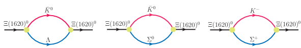
Figure 3: Self-energy of the $\Xi$(1620) state.

$$\Sigma_{\Xi(1620)}(k_{0}) =\sum_{Y=\Lambda,\Sigma^{0},\Sigma^{+}}({\cal{C}}_{Y})^{2}g^{2}_{\Xi(1620)\bar{K}Y}\int_{0}^{\infty}d\alpha\int_{0}^{\infty}d\eta$$

$$\times\frac{(-\frac{\Delta}{2z}k\!\!\!/_{0}+m_{Y})}{16\pi^{2}z^{2}}\exp\{-\frac{1}{\beta^{2}}[(-2\omega_{Y}^{2}-\eta$$

$$+\frac{\Delta^{2}}{4z})k_{0}^{2}+\alpha{}m_{Y}^{2}+\eta{}m^{2}_{\bar{K}}]\}.$$ (5)

where the $z=2+\alpha+\eta$ and $\Delta=-4\omega_{Y}-2\eta$. The $k_{0}^{2}=m^{2}_{\Xi(1620)}$ with $k_{0},m_{\Xi(1620)}$ denoting the four momenta and the mass of the $\Xi(1620)$, respectively, $k_{1}$, $m_{\bar{K}}$, and $m_{Y}$ are the four-momenta, the mass of the $\bar{K}$ meson, and the mass of the $Y$ baryon, respectively. Here, we set $m_{\Xi(1620)}=m_{Y}+m_{\bar{K}}-E_{b}$ with $E_{b}$ being the binding energy of $\Xi(1620)$. Isospin symmetry implies that

$${\cal{C}}_{Y}=\left\{\begin{aligned} 1&&{Y=\Lambda}\\ \sqrt{1/3}&&{Y=\Sigma^{0}}\\ -\sqrt{2/3}&&{Y=\Sigma^{+}}.\end{aligned}\right.$$ (6)

To estimate the radiative decays of the diagrams shown in Figs. (1-2), we need the effective Lagrangian densities related to the photon fields, which are Kim:2012pz ; Kim:2018qfu

$${\cal{L}}_{\gamma\Sigma\Sigma} =-\bar{\Sigma}[e_{\Sigma}A\!\!\!/-\frac{e{\kappa_{\Sigma}}}{2m_{N}}\sigma_{\mu\nu}\partial^{\nu}A^{\mu}]\Sigma,$$ (7)

$${\cal{L}}_{\gamma\Lambda\Lambda} =\frac{e\kappa_{\Lambda}}{2m_{N}}\bar{\Lambda}\sigma_{\mu\nu}\partial^{\nu}A^{\mu}\Lambda,$$ (8)

$${\cal{L}}_{\gamma\Sigma\Lambda} =\frac{e\mu_{\Sigma\Lambda}}{2m_{N}}\bar{\Sigma}^{0}\sigma_{\mu\nu}\partial^{\nu}A^{\mu}\Lambda,$$ (9)

$${\cal{L}}_{K^{*}K\gamma} =\frac{g_{K^{*+}K^{+}\gamma}}{4}e\epsilon^{\mu\nu\alpha\beta}F_{\mu\nu}K^{*+}_{\alpha\beta}K^{-}$$

$$+\frac{g_{K^{*0}K^{0}\gamma}}{4}e\epsilon^{\mu\nu\alpha\beta}F_{\mu\nu}K^{*0}_{\alpha\beta}\bar{K}^{0}+h.c.,$$ (10)

$${\cal{L}}_{KK\gamma} =ieA_{\mu}K^{-}\overleftrightarrow{\partial}^{\mu}K^{+}.$$ (11)

Where the strength tensor are defined as $\sigma_{\mu\nu}=\frac{i}{2}(\gamma_{\mu}\gamma_{\nu}-\gamma_{\nu}\gamma_{\mu})$, $F_{\mu\nu}=\partial_{\mu}A_{\nu}-\partial_{\nu}A_{\mu}$, and $K^{*}_{\mu\nu}=\partial_{\mu}K^{*}_{\nu}-\partial_{\nu}K^{*}_{\mu}$. The $M_{N}$ is the mass of the $p$ and $\alpha=e^{2}/4\pi=1/137$ is the electromagnetic fine structure constant. The anomalous and transition magnetic moments of the baryons are given by the PDG Zyla:2020zbs and are shown in Tab.(1)

Table 1: The anomalous and transition magnetic moments.

$\kappa_{\Sigma^{-}}=-0.16$	$\kappa_{\Sigma^{0}}=0.65$	$\kappa_{\Sigma^{+}}=1.46$
$\kappa_{\Lambda}=-0.61$	$\mu_{\Sigma\Lambda}=1.61$

The coupling constant $g_{K^{*+}K^{+}\gamma}$ and $g_{K^{*0}K^{0}\gamma}$ are introduced to get consistent results with experimental measurements of $K^{*+}\to{}K^{+}\gamma$ and $K^{*0}\to{}K^{0}\gamma$. The theoretical decay widths of $K^{*+}\to{}K^{+}\gamma$ and $K^{*0}\to{}K^{0}\gamma$ are

$$\Gamma(K^{*+}\to{}K^{+}\gamma)=\frac{\alpha{}g^{2}_{K^{*+}K^{+}\gamma}}{24}m_{K^{*+}}(m^{2}_{K^{*+}}-m^{2}_{K^{+}}),$$ (12)

$$\Gamma(K^{*0}\to{}K^{0}\gamma)=\frac{\alpha{}g^{2}_{K^{*0}K^{0}\gamma}}{24}m_{K^{*0}}(m^{2}_{K^{*0}}-m^{2}_{K^{0}}).$$ (13)

According to the experimental widths $\Gamma(K^{*+}\to{}K^{+}\gamma)=0.0503$ keV Zyla:2020zbs and $\Gamma(K^{*0}\to{}K^{0}\gamma)=0.125$ keV Zyla:2020zbs , the coupling constant $g_{K^{*}K\gamma}$ is fixed as

$$g_{K^{*+}K^{+}\gamma}=0.580~{}{\rm GeV^{-1}},~{}~{}~{}~{}~{}g_{K^{*0}K^{0}\gamma}=-0.904~{}{\rm GeV^{-1}},$$ (14)

and the signs of these coupling constants are fixed by the quark model.

In addition to the Lagrangians above, the meson-baryon interactions are also needed and can be obtained from the following chiral Lagrangians Garzon:2012np ; Oset:1997it

$${\cal{L}}_{VBB} =g(\langle\bar{B}\gamma_{\mu}[V^{\mu},B]\rangle+\langle\bar{B}\gamma_{\mu}B\rangle\langle{}V^{\mu}\rangle),$$ (15)

$${\cal{L}}_{PBB} =\frac{F}{2}\langle\bar{B}\gamma_{\mu}\gamma_{5}[u^{\mu},B]\rangle+\frac{D}{2}\langle\bar{B}\gamma_{\mu}\gamma_{5}\{u^{\mu},B\}\rangle,$$ (16)

$${\cal{L}}_{PBPB} =\frac{i}{4f^{2}}\langle\bar{B}\gamma^{\mu}[(P\partial_{\mu}P-\partial_{\mu}PP)B$$

$$-B(P\partial_{\mu}P-\partial_{\mu}PP)]\rangle$$ (17)

where $g=4.64$, $F=0.51$, $D=0.75$ Huang:2020taj ; Garzon:2012np ; Borasoy:1998pe and at the lowest order $u^{\mu}=-\sqrt{2}\partial^{\mu}P/f$ with $f=93$ MeV, and $\langle...\rangle$ denotes trace in the flavor space. The $B$,$P$, and $V^{\mu}$ are the $SU(3)$ pseudoscalar meson, vector meson, and baryon octet matrices, respectively, which are

$$B=\left(\begin{array}[]{ccc}\frac{1}{\sqrt{2}}\Sigma^{0}+\frac{1}{\sqrt{6}}\Lambda&\Sigma^{+}&p\\ \Sigma^{-}&-\frac{1}{\sqrt{2}}\Sigma^{0}+\frac{1}{\sqrt{6}}\Lambda&n\\ \Xi^{-}&\Xi^{0}&-\frac{2}{\sqrt{6}}\Lambda\\ \end{array}\right),$$ (18)

$$P=\left(\begin{array}[]{ccc}\frac{\pi^{0}}{\sqrt{2}}+\frac{\eta}{\sqrt{6}}&\pi^{+}&K^{+}\\ \pi^{-}&-\frac{\pi^{0}}{\sqrt{2}}+\frac{\eta}{\sqrt{6}}&K^{0}\\ K^{-}&\bar{K}^{0}&-\frac{2}{\sqrt{6}}\eta\end{array}\right),$$ (19)

$$V_{\mu}=\left(\begin{array}[]{cccc}\frac{1}{\sqrt{2}}(\rho^{0}+\omega)&\rho^{+}&K^{*+}\\ \rho^{-}&\frac{1}{\sqrt{2}}(-\rho^{0}+\omega)&K^{*0}\\ K^{*-}&\bar{K}^{*0}&\phi\\ \end{array}\right)_{\mu}.$$ (20)

Putting all the pieces together, we obtain the following decay amplitudes,

$${\cal{M}}_{a} (\Xi^{*0}\to\Xi^{0}\gamma)=i(i)^{3}\{\frac{(D-3F)\kappa_{\Lambda}}{2\sqrt{3}},\frac{(F+D)\mu_{\Sigma\Lambda}}{2}\}$$

$$\times{}\frac{eg_{\Xi^{*}\Lambda\bar{K}}}{4m_{N}f}\int\frac{d^{4}q}{(2\pi)^{4}}\Phi[(k_{1}\omega_{\Lambda}-k_{2}\omega_{\bar{K}^{0}})^{2}]$$

$$\times\bar{u}(p_{1})k\!\!\!/_{1}\gamma_{5}\frac{q\!\!\!/+m_{Y}}{q^{2}-m^{2}_{Y}}(\gamma_{\mu}p\!\!\!/_{2}-p\!\!\!/_{2}\gamma_{\mu})\frac{k\!\!\!/_{2}+m_{\Lambda}}{k_{2}^{2}-m^{2}_{\Lambda}}$$

$$\times{}u(p)\frac{1}{k_{1}^{2}-m^{2}_{\bar{K}^{0}}}\epsilon^{*\mu}(p_{2}),$$ (21)

$${\cal{M}}_{b} (\Xi^{*0}\to\Xi^{0}\gamma)=-i(i)^{3}e\frac{D+F}{\sqrt{2}f}C_{Y}g_{\Xi^{*}\Sigma^{+}\bar{K}^{-}}\int\frac{d^{4}q}{(2\pi)^{4}}$$

$$\times{}\Phi[(k_{1}\omega_{\Sigma^{+}}-k_{2}\omega_{\bar{K}^{-}})^{2}]\bar{u}(p_{1})k\!\!\!/_{1}\gamma_{5}$$

$$\times\frac{q\!\!\!/+m_{Y}}{q^{2}-m^{2}_{Y}}[\gamma_{\mu}+\frac{\kappa_{Y}}{4m_{N}}(\gamma_{\mu}p\!\!\!/_{2}-p\!\!\!/_{2}\gamma_{\mu})]$$

$$\times\frac{k\!\!\!/_{2}+m_{\Sigma^{+}}}{k_{2}^{2}-m^{2}_{\Sigma^{+}}}u(p)\frac{1}{k_{1}^{2}-m^{2}_{K^{-}}}\epsilon^{*\mu}(p_{2}),$$ (22)

$${\cal{M}}_{c} (\Xi^{*0}\to\Xi^{0}\gamma)=i(i)^{3}\{\frac{(D-3F)\mu_{\Sigma\Lambda}}{2\sqrt{3}},\frac{(F+D)\kappa_{\Sigma^{0}}}{2}\}$$

$$\times{}\frac{eg_{\Xi^{*}\Lambda\bar{K}}C_{Y}}{4m_{N}f}\int\frac{d^{4}q}{(2\pi)^{4}}\Phi[(k_{1}\omega_{\Sigma^{0}}-k_{2}\omega_{\bar{K}^{0}})^{2}]$$

$$\times\bar{u}(p_{1})k\!\!\!/_{1}\gamma_{5}\frac{q\!\!\!/+m_{Y}}{q^{2}-m^{2}_{Y}}(\gamma_{\mu}p\!\!\!/_{2}-p\!\!\!/_{2}\gamma_{\mu})\frac{k\!\!\!/_{2}+m_{\Sigma^{0}}}{k_{2}^{2}-m^{2}_{\Sigma^{0}}}$$

$$\times{}u(p)\frac{1}{k_{1}^{2}-m^{2}_{\bar{K}^{0}}}\epsilon^{*\mu}(p_{2}),$$ (23)

$${\cal{M}}^{K}_{d} (\Xi^{*0}\to\Xi^{0}\gamma)=-i(i)^{3}\frac{D+F}{\sqrt{2}f}eC_{Y}g_{\Xi^{*}\Sigma^{+}K^{-}}$$

$$\times{}\int\frac{d^{4}q}{(2\pi)^{4}}\Phi[(k_{1}\omega_{\Sigma^{+}}-k_{2}\omega_{{K}^{-}})^{2}]\bar{u}(p_{1})q\!\!\!/\gamma_{5}$$

$$\times{}\frac{k\!\!\!/_{2}+m_{\Sigma^{+}}}{k_{2}^{2}-m^{2}_{\Sigma^{+}}}u(p)\frac{1}{k_{1}^{2}-m^{2}_{K^{-}}}\frac{1}{q^{2}-m^{2}_{K^{+}}}$$

$$\times(q-k_{1})\cdot\epsilon^{*}(p_{2}),$$ (24)

$${\cal{M}}^{K^{*}}_{d} (\Xi^{*0}\to\Xi^{0}\gamma)=(i)^{3}\frac{egC_{Y}g_{K^{*}K\gamma}}{4}\int\frac{d^{4}q}{(2\pi)^{4}}$$

$$\times{}\Phi[(k_{1}\omega_{\Sigma^{+}}-k_{2}\omega_{{K}^{-}})^{2}]\bar{u}(p_{1})\gamma_{\rho}\frac{k\!\!\!/_{2}+m_{\Sigma^{+}}}{k_{2}^{2}-m^{2}_{\Sigma^{+}}}u(p)$$

$$\times{}\frac{1}{k_{1}^{2}-m^{2}_{K^{-}}}\frac{-g^{\rho\sigma}+q^{\rho}q^{\sigma}/m^{2}_{K^{*-}}}{q^{2}-m^{2}_{K^{*-}}}\epsilon^{\mu\nu\alpha\beta}$$

$$\times{}(p_{2\mu}g_{\nu\eta}-p_{2\nu}g_{\mu\eta})(q_{\alpha}g_{\beta\sigma}-q_{\beta}g_{\alpha\sigma})\epsilon^{*\eta}(p_{2}),$$ (25)

$${\cal{M}}_{e} (\Xi^{*0}\to\Xi^{0}\gamma)=(i)^{3}\frac{\sqrt{6}egC_{Y}g_{K^{*}K\gamma}}{8}\int\frac{d^{4}q}{(2\pi)^{4}}$$

$$\times{}\Phi[(k_{1}\omega_{\Lambda}-k_{2}\omega_{\bar{K}^{0}})^{2}]\bar{u}(p_{1})\gamma_{\rho}\frac{k\!\!\!/_{2}+m_{\Lambda}}{k_{2}^{2}-m^{2}_{\Lambda}}u(p)$$

$$\times{}\frac{1}{k_{1}^{2}-m^{2}_{\bar{K}^{0}}}\frac{-g^{\rho\sigma}+q^{\rho}q^{\sigma}/m^{2}_{\bar{K}^{*0}}}{q^{2}-m^{2}_{\bar{K}^{*0}}}\epsilon^{\mu\nu\alpha\beta}$$

$$\times{}(p_{2\mu}g_{\nu\eta}-p_{2\nu}g_{\mu\eta})(q_{\alpha}g_{\beta\sigma}-q_{\beta}g_{\alpha\sigma})\epsilon^{*\eta}(p_{2}),$$ (26)

$${\cal{M}}_{f} (\Xi^{*0}\to\Xi^{0}\gamma)=-(i)^{3}\frac{egC_{Y}g_{K^{*}K\gamma}}{4\sqrt{2}}\int\frac{d^{4}q}{(2\pi)^{4}}$$

$$\times{}\Phi[(k_{1}\omega_{\Sigma^{0}}-k_{2}\omega_{\bar{K}^{0}})^{2}]\bar{u}(p_{1})\gamma_{\rho}\frac{k\!\!\!/_{2}+m_{\Sigma^{0}}}{k_{2}^{2}-m^{2}_{\Sigma^{0}}}u(p)$$

$$\times{}\frac{1}{k_{1}^{2}-m^{2}_{\bar{K}^{0}}}\frac{-g^{\rho\sigma}+q^{\rho}q^{\sigma}/m^{2}_{\bar{K}^{*0}}}{q^{2}-m^{2}_{\bar{K}^{*0}}}\epsilon^{\mu\nu\alpha\beta}$$

$$\times{}(p_{2\mu}g_{\nu\eta}-p_{2\nu}g_{\mu\eta})(q_{\alpha}g_{\beta\sigma}-q_{\beta}g_{\alpha\sigma})\epsilon^{*\eta}(p_{2}),$$ (27)

where $\{{\cal{A}}$, and ${\cal{B}}\}$ are $\Lambda$ and $\Sigma$ baryon exchange,respectively. The amplitudes of the $\Xi^{0}(1620)\to\gamma\pi\Xi$ can be also easy obtained

$$\begin{split}{\cal{M}}_{a}&(\Xi^{*0}\to\pi^{0}\Xi^{0}\gamma,\pi^{+}\Xi^{-}\gamma)=i^{3}\frac{eC_{Y}g_{\Xi^{*}\bar{K}^{0}\Lambda}}{32m_{N}f^{2}}\left\{\begin{array}[]{ll}\{-\sqrt{3}\kappa_{\Lambda},\mu_{\Sigma\Lambda}\}\\ \{\sqrt{6}\kappa_{\Lambda},\sqrt{2}\mu_{\Sigma\Lambda}\}\\ \end{array}\right.\end{split}$$

$$\times{}\int\frac{d^{4}q}{(2\pi)^{4}}\Phi[(k_{1}\omega_{\Lambda}-k_{2}\omega_{\bar{K}^{0}})^{2}]\bar{u}(p_{1})k\!\!\!/_{1}\frac{q\!\!\!/+m_{Y}}{q^{2}+m^{2}_{Y}}$$

$$\times{}(\gamma_{\mu}p\!\!\!/_{2}-p\!\!\!/_{2}\gamma_{\mu})\frac{k\!\!\!/_{2}+m_{\Lambda}}{k_{2}^{2}-m^{2}_{\Lambda}}u(p)\epsilon^{*\mu}\frac{1}{k_{1}^{2}-m^{2}_{\bar{K}^{0}}},$$ (28)

$$\begin{split}{\cal{M}}_{b}&(\Xi^{*0}\to\pi^{0}\Xi^{0}\gamma,\pi^{+}\Xi^{-}\gamma)=i^{3}\frac{eC_{Y}g_{\Xi^{*}K^{-}\Sigma^{+}}}{4f^{2}}\left\{\begin{array}[]{ll}\frac{1}{\sqrt{2}}\\ 1\\ \end{array}\right.\end{split}$$

$$\times{}\int\frac{d^{4}q}{(2\pi)^{4}}\Phi[(k_{1}\omega_{\Sigma^{+}}-k_{2}\omega_{K^{-}})^{2}]\bar{u}(p_{1})k\!\!\!/_{1}\frac{q\!\!\!/+m_{Y}}{q^{2}+m^{2}_{Y}}$$

$$\times{}[\gamma_{\mu}+\frac{\kappa_{\Sigma^{+}}}{4m_{N}}(\gamma_{\mu}p\!\!\!/_{2}-p\!\!\!/_{2}\gamma_{\mu})]\frac{k\!\!\!/_{2}+m_{\Sigma^{+}}}{k_{2}^{2}-m^{2}_{\Sigma^{+}}}u(p)\epsilon^{*\mu}\frac{1}{k_{1}^{2}-m^{2}_{K^{-}}},$$ (29)

$$\begin{split}{\cal{M}}_{c}&(\Xi^{*0}\to\pi^{0}\Xi^{0}\gamma,\pi^{+}\Xi^{-}\gamma)=i^{3}\frac{eC_{Y}g_{\Xi^{*}K^{-}\Sigma^{+}}}{4f^{2}}\left\{\begin{array}[]{ll}\frac{1}{\sqrt{2}}\\ 1\\ \end{array}\right.\end{split}$$

$$\times{}\int\frac{d^{4}q}{(2\pi)^{4}}\Phi[(k_{1}\omega_{\Sigma^{+}}-k_{2}\omega_{K^{-}})^{2}]\bar{u}(p_{1})q\!\!\!/\frac{k\!\!\!/_{2}+m_{\Sigma^{+}}}{k_{2}^{2}+m^{2}_{\Sigma^{+}}}u(p)$$

$$\times{}(q^{\mu}+k^{\mu}_{1})\frac{1}{k_{1}^{2}-m^{2}_{K^{-}}}\frac{1}{q^{2}-m^{2}_{K^{-}}}\epsilon^{*}_{\mu},$$ (30)

$$\begin{split}{\cal{M}}_{d}&(\Xi^{*0}\to\pi^{0}\Xi^{0}\gamma,\pi^{+}\Xi^{-}\gamma)=i^{3}\frac{eC_{Y}g_{\Xi^{*}\bar{K}^{0}\Sigma^{0}}}{32m_{N}f^{2}}\left\{\begin{array}[]{ll}\{-\sqrt{3}\mu_{\Sigma\Lambda},\kappa_{\Sigma^{0}}\}\\ \{\sqrt{6}\mu_{\Sigma\Lambda},\sqrt{2}\kappa_{\Sigma^{0}}\}\\ \end{array}\right.\end{split}$$

$$\times{}\int\frac{d^{4}q}{(2\pi)^{4}}\Phi[(k_{1}\omega_{\Sigma^{0}}-k_{2}\omega_{\bar{K}^{0}})^{2}]\bar{u}(p_{1})k\!\!\!/_{1}\frac{q\!\!\!/+m_{Y}}{q^{2}+m^{2}_{Y}}$$

$$\times{}(\gamma_{\mu}p\!\!\!/_{2}-p\!\!\!/_{2}\gamma_{\mu})\frac{k\!\!\!/_{2}+m_{\Sigma^{0}}}{k_{2}^{2}-m^{2}_{\Sigma^{0}}}u(p)\epsilon^{*\mu}\frac{1}{k_{1}^{2}-m^{2}_{\bar{K}^{0}}},$$ (31)

$${\cal{M}}_{e} (\Xi^{*0}\to\bar{K}^{0}\Lambda\gamma)=-i\frac{e{\kappa_{\Lambda}}g_{\Xi^{*}\bar{K}^{0}\Lambda}C_{Y}}{4m_{N}}\Phi[(k_{1}\omega_{\Lambda}-k_{2}\omega_{\bar{K}^{0}})^{2}]$$

$$\times\bar{u}(p_{2})(\gamma^{\mu}p\!\!\!/_{1}-p\!\!\!/_{1}\gamma^{\mu})\frac{k\!\!\!/_{2}+m_{\Lambda}}{k_{2}^{2}-m^{2}_{\Lambda}}u(p)\epsilon^{*}_{\mu}(p_{1}),$$ (32)

$${\cal{M}}_{f} (\Xi^{*0}\to\bar{K}^{0}\Lambda\gamma)=-i\frac{e\mu_{\Sigma\Lambda}g_{\Xi^{*}\bar{K}^{0}\Sigma^{0}}C_{Y}}{4m_{N}}\Phi[(k_{1}\omega_{\Sigma^{0}}-k_{2}\omega_{\bar{K}^{0}})^{2}]$$

$$\times\bar{u}(p_{2})(\gamma^{\mu}p\!\!\!/_{1}-p\!\!\!/_{1}\gamma^{\mu})\frac{k\!\!\!/_{2}+m_{\Sigma^{0}}}{k_{2}^{2}-m^{2}_{\Sigma^{0}}}u(p)\epsilon^{*}_{\mu}(p_{1})$$ (33)

where the expressions in the curly brackets, $\left\{\begin{array}[]{ll}A\\ B\\ \end{array}\right.$, are for the $\Xi^{*0}\to\pi^{0}\Xi^{0}\gamma$ and $\Xi^{*0}\to\pi^{+}\Xi^{-}\gamma$, respectively.

With above, the total amplitudes of the $\Xi^{*0}\to\Xi^{0}\gamma$, $\Xi^{*0}\to\Xi^{0}\pi^{0}\gamma$, and $\Xi^{*0}\to\pi^{+}\Xi^{-}\gamma$ are the sum of these individual amplitudes, respectively,

$${\cal{M}}^{T}(\Xi^{*0}\to\Xi\gamma)=\sum_{i=a,b,c,d,e,f}{\cal{M}}_{i}(\Xi^{*0}\to\Xi\gamma),$$ (34)

$${\cal{M}}^{T}(\Xi^{*0}\to\pi\Xi\gamma)=\sum_{i=a,b,c,d}{\cal{M}}_{i}(\Xi^{*0}\to\pi\Xi\gamma),$$ (35)

$${\cal{M}}^{T}(\Xi^{*0}\to\bar{K}\Lambda\gamma)=\sum_{i=e.f}{\cal{M}}_{i}(\Xi^{*0}\to\bar{K}\Lambda\gamma).$$ (36)

Once the amplitudes are determined, the corresponding partial decay width can be easily obtained, which reads as,

$$d\Gamma(\Xi(1620)^{0} \to\gamma\Xi)=\frac{1}{2J+1}\frac{1}{32\pi^{2}}\frac{|\vec{p}_{1}|}{m^{2}_{\Xi^{*0}}}\bar{|{\cal{M}}|^{2}}d\Omega,$$ (37)

$$d\Gamma(\Xi(1620)^{0} \to\gamma\Xi\pi,\gamma\bar{K}\Lambda)=\frac{1}{2J+1}\frac{1}{(2\pi)^{5}}\frac{1}{16m^{2}}$$

$$\times{}\bar{|{\cal{M}}|^{2}}|\vec{p}^{*}_{3}||\vec{p}_{2}|dm_{13}d\Omega^{*}_{p_{3}}d\Omega_{p_{2}},$$ (38)

where $J$ is the total angular momentum of the $\Xi(1620)$, $|\vec{p}_{1}|$ is the three-momenta of the decay products in the center of mass frame, the overline indicates the sum over the polarization vectors of the final hadrons. The ($\vec{p}^{*}_{3},\Omega^{*}_{p_{3}}$) is the momentum and angle of the particle $\pi$ in the rest frame of $\pi$ and $\Xi$, and $\Omega_{p_{2}}$ is the angle of the photon in the rest frame of the decaying particle. The $m_{13}$ is the invariant mass for $\pi$ and $\Xi$ and $m_{\pi}+m_{\Xi}\leq{}m_{13}\leq{}m$.

III NUMERICAL RESULTS AND DISCUSSIONS

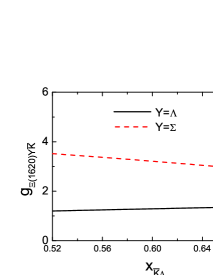
Figure 4: The $x_{\bar{K}\Lambda}$ dependence of $g_{\Xi^{*}(1620)\bar{K}\Lambda}$ and $g_{\Xi^{*}(1620)\bar{K}\Sigma}$.

To compute the radiative decay widths of the considered processes, the coupling constants of $\Xi^{*}(1620)$ to his components could be estimated by the compositeness conditions given by Eq. 4. Regarding the $\Xi^{*}(1620)$ as $S$-wave loosely $\bar{K}\Lambda$-$\bar{K}\Sigma$ hadronic molecule, the coupling constants $g_{\Xi^{*}(1620)\bar{K}\Lambda}$ and $g_{\Xi^{*}(1620)\bar{K}\Sigma}$ dependent on the parameter $x_{\bar{K}\Lambda}$ are plotted in Fig. 4. The parameter $x_{\bar{K}\Lambda}$ was constrained as $x_{\bar{K}\Lambda}=0.52-0.68$ by comparing the sum of the partial decay modes of $\Xi^{*}(1620)$ with the total width in our previous paper Huang:2020taj . It means that about $52\%-68\%$ of the total width comes from the $\bar{K}\Lambda$ channel, while the rest is provided by the $\bar{K}\Sigma$ channel. We find that the coupling constant $g_{\Xi^{*}(1620)\bar{K}\Lambda}$ monotonously increase with the increasing of the parameter $x_{\bar{K}\Lambda}$ in our consider $x_{\bar{K}\Lambda}$ range, while the coupling constant $g_{\Xi^{*}(1620)\bar{K}\Sigma}$ decline decreases with increasing $x_{\bar{K}\Lambda}$. The opposite trend can be easily understood, as the coupling constants $g_{\Xi^{*}(1620)\bar{K}\Lambda}$ and $g_{\Xi^{*}(1620)\bar{K}\Sigma}$ are directly proportional to the corresponding molecular compositions Dong:2009uf .

With obtained above coupling constants, the radiative decay width of the $\Xi(1620)^{0}$ into $\Xi^{0}\gamma$, $\Xi\gamma\pi$, and $\gamma\bar{K}\Lambda$ that are shown in Fig. 1 and Fig. 2 can be calculated straightforwardly. However, the amplitudes of the $\Xi(1620)^{0}\to\gamma\Xi^{0}$ and $\Xi(1620)^{0}\to\gamma\Xi\pi$ cannot satisfy the gauge invariance of the photon field. To ensure the gauge invariance of the total amplitudes, the contact diagram must be included as well. The corresponding Feynman diagrams are shown in Fig. 5.

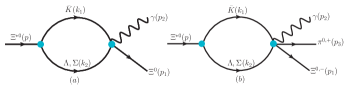
Figure 5: Contact diagram for $\Xi^{*0}\to\Xi^{0}\gamma$, $\Xi^{*0}\to\Xi^{0}\pi^{0}\gamma$, and $\Xi^{*0}\to\pi^{+}\Xi^{-}\gamma$. We also show definitions of the kinematics ($p_{1},p_{2},p_{3},k_{1},k_{2}$, and $p$) used in the calculation.

For the present calculation, we adopt the following form to satisfy $p_{2}^{\mu}{\cal{M}}^{Total}_{\mu}(\equiv{{\cal{M}}}^{T}+{\cal{M}}_{com})=0$

$${\cal{M}}^{a}_{com}(\Xi^{*}\to\gamma\Xi^{0})=\frac{D+F}{\sqrt{2}f}eC_{Y}g_{\Xi^{*}\Sigma^{+}K^{-}}\int_{0}^{\infty}d\alpha\int_{0}^{\infty}d\eta$$

$$\times\int_{0}^{\infty}d\zeta\frac{1}{16\pi^{2}y^{2}\beta^{2}}\bar{u}(p_{1})({\cal{C}}_{1}^{\mu}{\cal{T}}_{1}+{\cal{C}}_{2}^{\mu}{\cal{T}}_{2})\gamma_{5}u(p)\epsilon^{*}_{\mu}(p_{2}),$$ (39)

$$\begin{split}&{\cal{M}}^{b}_{com}(\Xi^{*0}\to\pi^{0}\Xi^{0}\gamma,\pi^{+}\Xi^{-}\gamma)=-i^{3}\frac{eC_{Y}g_{\Xi^{*}K^{-}\Sigma^{+}}}{4f^{2}}\left\{\begin{array}[]{ll}\frac{1}{\sqrt{2}}\\ 1\\ \end{array}\right.\end{split}$$

$$\times\int_{0}^{\infty}d\alpha\int_{0}^{\infty}d\eta\int_{0}^{\infty}d\zeta\frac{1}{16\pi^{2}y^{2}\beta^{2}}$$

$$\times\bar{u}(p_{1})({\cal{D}}_{1}^{\mu}{\cal{T}}_{1}+{\cal{D}}_{2}^{\mu}{\cal{T}}_{2})u(p)\epsilon^{*}_{\mu}(p_{2}).$$ (40)

Where

$${\cal{T}}_{1} =\exp\{-\frac{1}{\beta^{2}}[\alpha(-p_{1}^{2}+m^{2}_{K^{-}})+\eta{}m_{\Sigma^{+}}^{2}+\zeta(-p_{2}^{2}+m^{2}_{\Sigma^{+}})$$

$$-(p_{1}\omega_{\Sigma^{+}}-p_{2}\omega_{K^{-}})^{2}+\frac{1}{4z}({\cal{H}}_{2}p_{2}-{\cal{H}}_{1}p_{1})^{2}]\},$$ (41)

$${\cal{T}}_{2} =\exp\{-\frac{1}{\beta^{2}}[\alpha(-p_{2}^{2}+m^{2}_{K^{-}})+\eta{}m_{K^{-}}^{2}+\zeta(-p_{1}^{2}+m^{2}_{\Sigma^{+}})$$

$$-(p_{2}\omega_{\Sigma^{+}}-p_{1}\omega_{K^{-}})^{2}+\frac{1}{4z}({\cal{H}}_{2}p_{1}-{\cal{H}}_{1}p_{2})^{2}]\},$$ (42)

$${\cal{C}}_{1}^{\mu} =-\frac{m_{1}^{2}{\cal{H}}_{1}^{3}}{8y^{3}}(2p_{1}^{\mu}-m_{1}\gamma^{\mu})-\frac{m_{1}^{3}{\cal{H}}_{1}^{2}}{4y^{2}}\gamma^{\mu}+\frac{m_{1}^{2}{\cal{H}}_{1}^{2}}{2y^{2}}p_{1}^{\mu}$$

$$-\frac{m_{1}m^{2}_{\Sigma^{+}}{\cal{H}}_{1}}{2y}\gamma^{\mu}+m_{1}m^{2}_{\Sigma^{+}}\gamma^{\mu}+\frac{m_{1}m_{\Sigma^{+}}{\cal{H}}^{2}_{1}}{2y^{2}}p_{1}^{\mu}$$

$$+(\frac{(m+m_{1})m_{\Sigma^{+}}{\cal{H}}_{1}{\cal{H}}_{2}}{2y^{2}}-\frac{m_{1}m_{\Sigma^{+}}{\cal{H}}_{1}}{y})p_{1}^{\mu}-\frac{m_{\Sigma^{+}}-m_{1}}{y}\gamma^{\mu}$$

$$+\frac{{\cal{H}}_{1}^{2}{\cal{H}}_{2}}{4y^{3}}p_{1}\cdot{}p_{2}(2p_{1}^{\mu}-m_{1}\gamma^{\mu})+\frac{m_{1}{\cal{H}}_{1}{\cal{H}}_{2}}{2y^{2}}p_{1}\cdot{}p_{2}\gamma^{\mu}$$

$$+\frac{(m+m_{1})m_{1}{\cal{H}}_{1}{\cal{H}}_{2}}{2y^{2}}p_{1}^{\mu}+\frac{3{\cal{H}}_{1}}{2y^{2}}(2p_{1}^{\mu}-m_{1}\gamma^{\mu}),$$ (43)

$${\cal{C}}_{2}^{\mu} =-\frac{m_{1}^{2}{\cal{H}}_{2}^{3}}{4y^{3}}p_{1}^{\mu}-\frac{m_{1}^{2}{\cal{H}}_{2}^{2}}{4y^{2}}p_{1}^{\mu}-\frac{(m+m_{1})m_{\Sigma^{+}}{\cal{H}}_{1}{\cal{H}}_{2}}{2y^{2}}p_{1}^{\mu}$$

$$-\frac{(m+m_{1})m_{\Sigma^{+}}{\cal{H}}_{1}}{2y}p_{1}^{\mu}-\frac{m_{1}m_{\Sigma^{+}}{\cal{H}}^{2}_{2}}{2y^{2}}p_{1}^{\mu}-\frac{m_{1}m_{\Sigma^{+}}{\cal{H}}_{2}}{2y}p_{1}^{\mu}$$

$$+\frac{m_{\Sigma^{+}}}{y}\gamma^{\mu}+\frac{{\cal{H}}_{1}{\cal{H}}^{2}_{2}}{2y^{3}}p_{1}\cdot{}p_{2}p_{1}^{\mu}+\frac{{\cal{H}}_{1}{\cal{H}}_{2}}{2y^{2}}p_{1}\cdot{}p_{2}p_{1}^{\mu}$$

$$-\frac{m_{1}(m+m_{1}){\cal{H}}^{2}_{2}}{2y^{2}}p_{1}^{\mu}-\frac{m_{1}(m+m_{1}){\cal{H}}_{2}}{2y}p_{1}^{\mu}$$

$$+\frac{{\cal{H}}_{2}}{2y^{2}}(2p_{1}^{\mu}-m_{1}\gamma^{\mu})+\frac{m_{1}{\cal{H}}_{2}}{2y^{2}}\gamma^{\mu}+\frac{2{\cal{H}}_{2}}{y^{2}}p_{1}^{\mu}+\frac{2}{y}p_{1}^{\mu},$$ (44)

$${\cal{D}}_{1}^{\mu} =(-\frac{m^{2}_{\Sigma^{+}}{\cal{H}}_{1}}{2y}+m^{2}_{\Sigma^{+}})(2p^{\mu}-m\gamma^{\mu})-\frac{m_{\Sigma^{+}}{\cal{H}}_{1}^{2}}{2y^{2}}(m-p\!\!\!/_{2})p^{\mu}$$

$$+\frac{m_{\Sigma^{+}}{\cal{H}}_{1}{\cal{H}}_{2}}{2y^{2}}p\!\!\!/_{2}p^{\mu}+\frac{m_{\Sigma^{+}}{\cal{H}}_{1}}{y}(m-p\!\!\!/_{2})p^{\mu}+\frac{m_{\Sigma^{+}}}{y}\gamma^{\mu}$$

$$-\frac{mm_{13}^{2}{\cal{H}}^{3}_{1}}{8y^{3}}\gamma^{\mu}+\frac{m(m^{2}-m^{2}_{13}){\cal{H}}^{2}_{1}{\cal{H}}_{2}}{8y^{3}}\gamma^{\mu}-\frac{m^{2}_{13}{\cal{H}}^{2}_{1}}{4y^{2}}$$

$$\times(2p^{\mu}-m\gamma^{\mu})+\frac{{\cal{H}}^{2}_{1}m^{2}_{13}}{2y^{2}}p^{\mu}+(\frac{{\cal{H}}_{1}{\cal{H}}_{2}(m^{2}-m^{2}_{13})}{4y^{2}}+\frac{1}{y})$$

$$\times(2p^{\mu}-m\gamma^{\mu})-\frac{m{\cal{H}}_{1}{\cal{H}}_{2}}{2y^{2}}p\!\!\!/_{2}p^{\mu}+\frac{3m{\cal{H}}_{1}}{2y^{2}}\gamma^{\mu},$$ (45)

$${\cal{D}}_{2}^{\mu} =-\frac{m_{\Sigma^{+}}{\cal{H}}_{1}{\cal{H}}_{2}}{2y^{2}}p\!\!\!/_{2}p^{\mu}+\frac{m_{\Sigma^{+}}{\cal{H}}^{2}_{2}}{2y^{2}}(m-p\!\!\!/_{2})p^{\mu}-\frac{m_{\Sigma^{+}}}{y}\gamma^{\mu}$$

$$+\frac{(m^{2}-m_{13}^{2}){\cal{H}}_{1}{\cal{H}}_{2}^{2}}{4y^{3}}p^{\mu}-\frac{m{\cal{H}}_{1}{\cal{H}}_{2}}{2y^{2}}p\!\!\!/_{2}p^{\mu}-\frac{m^{2}_{13}{\cal{H}}_{2}^{3}}{4y^{3}}p^{\mu}$$

$$+\frac{m^{2}_{13}{\cal{H}}_{2}^{2}}{2y^{2}}p^{\mu}+\frac{3{\cal{H}}_{2}}{y^{2}}p^{\mu}-\frac{m}{y}\gamma^{\mu}.$$ (46)

with $y=1+\alpha+\eta+\zeta$,${\cal{H}}_{2}=2(\zeta+\omega_{K^{-}})$,${\cal{H}}_{1}=2(\alpha+\omega_{\Sigma^{+}})$, and $m^{2}_{13}=(p_{1}+p_{3})^{2}$. $m$ and $m_{1}$ are the masses of the $\Xi^{*}$ and $\Xi$, respectively.

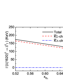
Figure 6: Decomposed contributions to the decay width of the $\Xi(1620)^{0}$ into $\Xi^{0}\gamma$.

With obtained the total amplitude, the radiative decay width of the $\Xi(1620)^{0}$ into $\Xi^{0}\gamma$ can be calculated straightforwardly. The dependence of the corresponding radiative decay width on $x_{\bar{K}\Lambda}$ is given in Fig. 6. The $x_{\bar{K}\Lambda}$ value within a reasonable range from 0.52 to 0.68, the radiative decay width of the $\Xi(1620)^{0}\to\gamma\Xi^{0}$ contribution from the $\bar{K}\Sigma$ channel monotonously decreases. However, it increases for the $\bar{K}\Lambda$ channel contribution to the $\Xi(1620)^{0}\to\gamma\Xi^{0}$. Moreover, the $\bar{K}\Sigma$ component provides the dominant contribution to the partial decay width of the $\gamma\Xi^{0}$ two-body channel. The $\bar{K}\Lambda$ contribution to the $\gamma\Xi^{0}$ two-body channel is very small. This is different from our results in Ref. Huang:2020taj that the $\bar{K}\Lambda$ component provides the dominant contribution to the strong decay width of the $\Xi(1620)$. A possible explanation for these may be that the interaction between the $\Sigma$ baryon and photon is stronger than $\gamma{}-\Lambda$ interaction because since the $\Sigma^{0}$ decays completely to the final state containing $\Lambda$ baryon and $\gamma$ Zyla:2020zbs .

Fig. 6 also tell us that the total radiative decay width decrease for the $\Xi(1620)^{0}\to\gamma\Xi^{0}$ when the $x_{\bar{K}\Lambda}$ is changed from 0.52 to 0.68. We also find that the interference between the $\bar{K}\Sigma$ channel and $\bar{K}\Lambda$ channel is quite small, leading to a total decay width of the $\Xi(1620)^{0}\to\gamma\Xi^{0}$ mainly contribution from the $\bar{K}\Sigma$ channel. This does not alter the conclusion that the $\bar{K}\Lambda$ channel strongly couples to the $\bar{K}\Sigma$ channel Ramos:2002xh ; Huang:2020taj . The main reason for this is that the radiative decay widths are often in the keV regime and are far less than their strong counterparts. Indeed, the total radiative decay width for the $\Xi(1620)^{0}\to\gamma\Xi^{0}$ is predicted to be $118.76-174.21$ KeV, which is far less than the total decay width is predicted to be about 50.39-68.79 MeV Huang:2020taj .

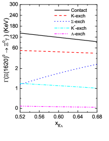
Figure 7: (color online) The partial decay widths from $K^{-}$(red dash line), $\bar{K}^{*}$(cyan dash dot line), $\Sigma$ (blue dot line), $\Lambda$(magenta dash dot dot line), and the remainder is the contact term exchange contribution for the $\Xi(1620)^{0}\to\gamma\Xi^{0}$ as a function of the parameter $x_{\bar{K}\Lambda}$.

The individual contributions of $K^{-}$, $\bar{K}^{*}$, $\Sigma$, $\Lambda$ exchanges, and contact term for the reaction $\Xi(1620)^{0}\to\gamma\Xi^{0}$ are shown in Fig. 7. The amplitudes corresponding to the $K^{-}$-exchange and $\Sigma^{+}$-exchange are not gauge invariant, while the rest is gauge invariant. One can see that the contract term and $K^{-}$-exchange provide a dominant contribution to the total decay width, and is at last sixty orders of magnitude bigger than those of the amplitudes corresponding to the $\bar{K}^{*}$, $\Sigma$, and $\Lambda$ exchanges for the $x_{\bar{K}\Lambda}$ range studied.

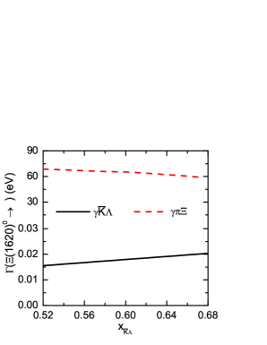
Figure 8: (color online) The partial decay widths of the $\Xi(1620)^{0}\to\gamma\Xi\pi$ and $\Xi(1620)^{0}\to\gamma\bar{K}\Lambda$.

Now we turn to the three-body radiative decays $\Xi(1620)^{0}\to\gamma\pi\Xi$ and $\Xi(1620)^{0}\to\gamma\bar{K}\Lambda$. The decay widths with varying $x_{\bar{K}\Lambda}$ from 0.52 to 0.68 for such two transitions are presented in Fig. 8. Since the phase space is small compared with the two-body radiative decay channel $\Xi(1620)^{0}\to\gamma\Xi^{0}$, the decay width should be the smallest for the $\Xi(1620)^{0}\to\gamma\bar{K}\Lambda$ channel, should be intermediate for the $\Xi(1620)^{0}\to\gamma\pi\Xi$ channel, and should be biggest for the $\Xi(1620)^{0}\to\gamma\Xi^{0}$ channel. Indeed, our study shows that the partial width of $\Xi(1620)^{0}\to\gamma\bar{K}\Lambda$ is rather small, weakly increasing with the $x_{\bar{K}\Lambda}$ increasing. In particular, the partial width varies from 0.016 to 0.020 eV in the $x_{\bar{K}\Lambda}$ range studied. However, the partial width of the $\Xi(1620)^{0}\to\gamma\Xi\pi$ decreases with the increase of $x_{\bar{K}\Lambda}$ and the partial width of the $\Xi(1620)^{0}\to\gamma\Xi\pi$ is estimated to be $68.75-58.19$ eV.

IV SUMMARY

We studied the two-body and three-body radiative decays of the $\Xi(1620)$ state assuming that it is a bound state of $\bar{K}\Lambda$-$\bar{K}\Sigma$. The coupling of $\Xi(1620)$ to his components are fixed by the Weinberg compositeness condition. The radiative decays for the $\Xi(1620)^{0}\to\gamma\Xi^{0}$ and $\Xi(1620)^{0}\to\gamma\pi\Xi$ are via triangle diagrams with exchanges of a pseudoscalar meson $K$, vector meson $K^{*}$, and baryon $\Sigma$ and $\Lambda$. The three body decay for the $\Xi(1620)^{0}\to\gamma\bar{K}\Lambda$ happen at tree level. In the relevant parameter region, the partial widths are evaluated as

$$\Gamma(\Xi(1620)^{0}\to\gamma\Xi^{0})=118.76-174.21~{}\rm{KeV},$$

$$\Gamma(\Xi(1620)^{0}\to\gamma\Xi\pi)=58.19-68.75~{}\rm{eV},$$ (47)

$$\Gamma(\Xi(1620)^{0}\to\gamma\bar{K}\Lambda)=0.016-0.020~{}\rm{eV}.$$

Future experimental measurements of these processes can be useful to test the molecule interpretations of the $\Xi(1620)$. Based on the current integrated luminosity and our estimations, facilities such as the LHCb might be able to detect radiative decays of the baryon in the keV regime. This research can also be performed in the forthcoming Belle II experiment.

References

(1)
P. A. Zyla et al. [Particle Data Group],
Review of Particle Physics,
PTEP 2020,083C01 (2020).
(2)
M. Sumihama et al. [Belle Collaboration],
Phys. Rev. Lett. 122, 072501 (2019).
(3)
R. T. Ross, T. Buran, J. L. Lloyd, J. H. Mulvey and D. Radojicic,
Phys. Lett. 38B, 177 (1972).
(4)
E. Briefel et al.,
Phys. Rev. D 16, 2706 (1977).
(5)
S. Capstick and N. Isgur,
Phys. Rev. D 34, 2809 (1986)
[AIP Conf. Proc. 132, 267 (1985)].
(6)
W. H. Blask, U. Bohn, M. G. Huber, B. C. Metsch and H. R. Petry,
Z. Phys. A 337, 327 (1990).
(7)
Y. I. Azimov, R. A. Arndt, I. I. Strakovsky and R. L. Workman,
Phys. Rev. C 68, 045204 (2003).
(8)
A. Ramos, E. Oset and C. Bennhold,
Phys. Rev. Lett. 89, 252001 (2002).
(9)
C. Garcia-Recio, M. F. M. Lutz and J. Nieves,
Phys. Lett. B 582, 49 (2004).
(10)
D. Gamermann, C. Garcia-Recio, J. Nieves and L. L. Salcedo,
Phys. Rev. D 84, 056017 (2011).
(11)
K. Miyahara, T. Hyodo, M. Oka, J. Nieves and E. Oset,
Phys. Rev. C 95,035212 (2017).
(12)
Y. Oh,
Phys. Rev. D 75, 074002 (2007).
(13)
Z. Y. Wang, J. J. Qi, J. Xu and X. H. Guo,
Eur. Phys. J. C 79, 640 (2019).
(14)
K. Chen, R. Chen, Z. F. Sun and X. Liu,
Phys. Rev. D 100, 074006 (2019).
(15)
Y. Huang and L. Geng,
Eur. Phys. J. C 80, 837 (2020).
(16)
R. Koniuk and N. Isgur,
Phys. Rev. D 21, 1868 (1980)
[erratum: Phys. Rev. D 23, 818 (1981)].
(17)
Y. Huang, C. j. Xiao, L. S. Geng and J. He,
Phys. Rev. D 99, 014008 (2019).
(18)
Y. Dong, A. Faessler, T. Gutsche and V. E. Lyubovitskij,
Phys. Rev. D 81, 074011 (2010).
(19)
Y. Huang, M. Z. Liu, Y. W. Pan, L. S. Geng, A. Martínez Torres and K. P. Khemchandani,
Phys. Rev. D 101, 014022 (2020).
(20)
A. Faessler, T. Gutsche, V. E. Lyubovitskij and Y. L. Ma,
Phys. Rev. D 76, 114008 (2007).
(21)
Y. Dong, A. Faessler, T. Gutsche, S. Kovalenko and V. E. Lyubovitskij,
Phys. Rev. D 79, 094013 (2009).
(22)
Y. Dong, A. Faessler, T. Gutsche and V. E. Lyubovitskij,
J. Phys. G 38, 015001 (2011).
(23)
Y. Dong, A. Faessler and V. E. Lyubovitskij,
Prog. Part. Nucl. Phys. 94, 282 (2017).
(24)
C. J. Xiao, Y. Huang, Y. B. Dong, L. S. Geng and D. Y. Chen,
Phys. Rev. D 100, 014022 (2019).
(25)
Y. Huang, C. j. Xiao, Q. F. Lü, R. Wang, J. He and L. Geng,
Phys. Rev. D 97, 094013 (2018).
(26)
S. H. Kim, S. i. Nam, A. Hosaka and H. C. Kim,
Phys. Rev. D 88, 054012 (2013).
(27)
S. H. Kim and H. C. Kim,
Phys. Lett. B 786, 156 (2018).
(28)
E. J. Garzon and E. Oset,
Eur. Phys. J. A 48, 5 (2012).
(29)
E. Oset and A. Ramos,
Nucl. Phys. A 635, 99-120 (1998).
(30)
B. Borasoy,
Baryon axial currents,
Phys. Rev. D 59, 054021 (1999).