Spatial-spectral Terahertz Networks

Abstract

This paper focuses on the spatial-spectral terahertz (THz) networks, where transmitters equipped with leaky-wave antennas send information to their receivers at the THz frequency bands. As a directional and nearly planar antenna, the leaky-wave antenna allows for information transmissions with narrow beams and high antenna gains. The conventional large antenna arrays are confronted with challenging issues such as scaling limits and path discovery in the THz frequencies. Therefore, this work exploits the potential of leaky-wave antennas in the dense THz networks, to establish low-complexity THz links. By addressing the propagation angle-frequency coupling effects, the transmission rate is analyzed. The results show that the leaky-wave antenna is efficient for achieving the high-speed transmission rate. The co-channel interference management is unnecessary when the THz transmitters with large subchannel bandwidths are not extremely dense. A simple subchannel allocation solution is proposed, which enhances the transmission rate compared with the same number of subchannels with the equal allocation of the frequency band. After subchannel allocation, a low-complexity power allocation method is proposed to improve the energy efficiency.

I Introduction

The emerging services such as edge computing, immersive communication and tactile internet demand high-speed data transmissions. In an attempt to achieve these services, large millimeter wave (mmWave) frequency bands have been leveraged in 5G (currently 24-50 GHz [1]). However, with the increasing numbers of smart devices and autonomous vehicles in the Internet-of-Things, more bandwidths are always required to strengthen the ultra-reliable and low latency communications (URLLC). Since the terahertz (THz) frequency bands are abundant, THz communication is viewed as a promising 6G technology for reaching unprecedentedly high data rates [2, 3, 4].

In order to counteract the severe path losses in the higher frequencies, large antenna arrays with narrow beams have been adopted in 5G and its evolution [5]. In light of sparse-scattering mmWave channel environments, hardware costs and power consumptions etc., analog beamforming or hybrid beamforming approaches are recommended in the mmWave systems [5, 6]. The implementations of antenna arrays in the THz communications are investigated in [7, 8, 9, 10, 11], where various beamforming/precoding designs are proposed. However, using conventional antenna arrays has encountered many challenging issues in the THz frequencies, e.g., array architecture for accommodating highly dense THz antennas [3], phase modulation technique for developing THz phase shifters [12, 13], and path discovery [14]. In addition, efficient feed network designs [15] and beam squint mitigation [16] may also be required for developing wideband THz phased arrays. Therefore, it is essential to appropriately choose the THz antennas without adding significant link budgets and power consumptions [4, 8].

The leaky-wave antenna enables the wave to travel along the guiding architecture, in order to intensify the radio energy in preferred directions [17, 18, 19]. As a low-cost and easy-to-manufacture traveling-wave antenna, the leaky-wave antenna can provide frequency-dependent narrow beams with high antenna gains [19] and frequency-scanning capability [20, 21]. It has been utilized in many areas including frequency-division multiplexing THz communication [22], THz radar sensing [23, 24, 25], and physical layer security enhancement [26]. Different from the beam management with conventional large arrays in which an exhaustive search for the best beam is required [27], the extensive beam training in the THz link discovery with leaky-wave antennas is unnecessary [14, 28]. One key feature of the leaky-wave antenna is that it enables the information transmissions in a spatial-spectral manner, i.e., frequencies are correlated with the transmission directions. There are also other directional antenna designs such as horn and lens antennas. In particular, horn antenna has been used in the mmWave and THz channel measurements [29, 3] and fixed wireless access for THz communication systems [2]. Unlike leaky-wave antenna, these antennas are inherently fixed beam solution with a single direction, and integrating them for expanding coverage needs to be properly addressed [4].

The aforementioned works only study the case of point-to-point THz communication with leaky-wave antenna [22, 26]. When there exist large numbers of transceivers in the THz networks with massive connections, the co-channel interference has an adverse effect on the transmission rate, which has to be evaluated. Moreover, THz transmissions utilize much larger frequency bandwidths, and subchannel allocation plays an essential role in controlling the number of subchannels while guaranteeing the targeted performance, to keep the peak-to-average power ratio (PAPR) at a low level. Unfortunately, few research contributions investigate the subchannel allocation when applying the leaky-wave antenna in the THz communications. In addition, energy efficiency enhancement is of importance, to reduce power consumption. Therefore, we adopt the leaky-wave antennas to harness the THz waves in the dense THz networks, and the main contributions are concluded as follows:

• THz Networks with Leaky-wave Antennas: In the considered THz networks, each transmitter equipped with a leaky-wave antenna (TE₁ mode) sends information to its corresponding receiver with an omnidirectional antenna. Since none-line-of-sight (NLoS) links heavily depend on the reflectors in the THz frequencies [3, 30, 31] and the interference from NLoS links in dense THz networks can be negligible similar to the dense mmWave networks [32], we focus on the dominant line-of-sight (LoS) links. As a useful tool to evaluate the performance behavior in large-scale wireless networks [33], stochastic geometry is employed to model the spatial distributions of transmitters.

• Average Transmission Rate and Subchannel Allocation: In light of the spatial energy distribution under the leaky-wave antenna radiation, the average transmission rate is quantified for an arbitrary THz subchannel. Considering the fact that different THz frequencies have different subchannel bandwidths and undergo distinct channel conditions, a closed-form solution for subchannel allocation is proposed to enhance the transmission rate with the minimum number of subchannels. Then, a low-complexity power allocation is designed to maximize the average energy efficiency (EE) over the number of subchannels.

• Design Insights: Our results show that high-speed transmission rates are achievable in the dense THz networks with leaky-wave antennas, and noise-limited phenomenon occurs when the transmitters are not super dense. The average transmission rate can vary dramatically with slightly different values of aperture length or attenuation coefficient. The proposed subchannel allocation improves the average transmission rate in the leaky-wave antenna systems, compared with the same number of subchannels with the equal allocation of the frequency band. Our power allocation method can improve the EE. It is demonstrated that center frequencies with the maximum radiated energy may not be the best option when ignoring the channel gains. The slight increase in the attenuation coefficient can dramatically improve the average transmission rate for large frequency bandwidths, since more frequencies are in the main-lobe that captures large radiated energy.

The rest of this paper is organized as follows. The considered system model is described in Section II, and the average transmission rate is analyzed based on stochastic geometry in Section III. Subchannel allocation is determined in Section IV. Section V focuses on the EE enhancement. Section VI covers the simulation results. Finally, some concluding remarks are presented in Section VII.

II System Descriptions

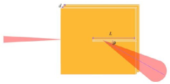
Figure 1: An illustration of leaky-wave antenna with the lowest transverse-electric (TE₁) mode.

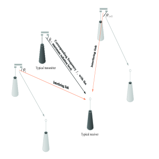
Figure 2: An illustration of THz network with leaky-wave antennas, where the interfering antenna gains depend on the propagation angles and the frequencies of the interfering links.

As shown in Fig. 1, the guiding structure of a 1D leaky-wave antenna consists of a rectangular waveguide with a longitudinal slit, where $d$, $L$ and $\theta$ denote the inter-plate distance, aperture length and propagation angle, respectively. In the large-scale THz networks illustrated by Fig. 2, each transmitter equipped with a leaky-wave antenna communicates with its corresponding receiver equipped with an omnidirectional antenna (namely single-input single-output), and they are randomly located following a homogeneous Poisson point process (PPP) $\Phi_{\rm THz}$ with density $\lambda_{\rm THz}$.

Given a THz frequency $f$ and the propagation angle $\theta\left(0<\theta<90^{o}\right)$, the far-field radiation pattern of the considered leaky-wave antenna is given by [34]

$$G\left(f,\theta\right)=L\mathrm{sinc}\left[\left(-j\alpha-k_{0}\cos\theta+\beta\right)\frac{L}{2}\right],$$ (1)

where $j=\sqrt{-1}$, $\alpha$ is the attenuation coefficient resulting from the power absorption in the structure, $k_{0}=2\pi f/c$ with the speed of light $c$ is the wavenumber of the free-space, $\beta=k_{0}\sqrt{1-\left(\frac{f_{\rm co}}{f}\right)^{2}}$ is the phase constant of the TE₁ mode based traveling wave, in which $f_{\rm co}=\frac{c}{2d}$ is the cutoff frequency [35]. The available frequencies should be higher than the cutoff frequency (i.e., $f>f_{\rm co}$), to enable that THz wave propagates away from the antenna structure, namely fast wave radiation [34]. Given a LoS direction $\theta$ of a receiver, the maximum level of the radiation can be achieved by using the the following frequency [19, 22]:

$$f^{\max}\left(\theta\right)=\frac{f_{\rm co}}{\sin\theta}.$$ (2)

As shown in Fig. 3, the frequency for maximizing the radiation is reliant on the beam angle, and lowering attenuation coefficient results in a narrower beam.

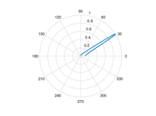
(a) $f=80$GHz, $\alpha=30$rad/m

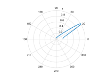
(b) $f=80$GHz, $\alpha=60$rad/m

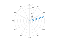
(c) $f=160$GHz, $\alpha=30$rad/m

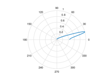
(d) $f=160$GHz, $\alpha=60$rad/m

Figure 3: Examples of the leaky-wave antenna’s radiation pattern with $L=5.5$cm and $d=3.5$mm.

Although transmitters may have different propagation angles and send information messages with the maximum antenna gains in the different THz frequencies based on (2), co-channel interference still exists in the large-scale THz networks, where the nearby transceivers may use the same subchannels for the low propagation angle difference $\Delta\theta$. As measured in [22], for a given $\Delta\theta$, its corresponding frequency bandwidth is

$$B\left(\theta\right)=\frac{f_{\rm co}\Delta\theta}{\sin\theta\tan\theta},$$ (3)

which can be interpreted as the range of the frequencies whose levels of radiation are close to the frequency $f^{\max}\left(\theta\right)$. In addition, different transmitters may have different cutoff frequencies and propagation angles, however, they may leverage the same frequency band, as indicated in (2). Therefore, the transmission rate of a subchannel at a typical receiver (at the origin) can be expressed as

$$R_{o}=B_{o}\log_{2}\left(1+\frac{{q_{t}\widetilde{G}\left({f_{o},\theta_{o}}\right)\ell\left(r_{o}\right)}}{{\sum\nolimits_{i\in\widetilde{\Phi}_{\rm THz}/o}{q_{t}\widetilde{G}\left({f_{i},\varphi_{i}}\right)\ell\left(r_{i}\right)}+\sigma_{o}^{2}}}\right),$$ (4)

where $B_{o}$ is the subchannel bandwidth, $q_{t}$ is the transmit power spectral density (PSD), $\widetilde{G}\left({f,\theta}\right)=\xi G\left(f,\theta\right)$ with a constant $\xi$ is the effective antenna gain, $\theta_{o}$ is the typical propagation angle, $\ell\left(r\right)$ is the path loss function with the communication distance $r$, $f_{o}$ and $f_{i}$ are the frequencies used by the typical transmitter and the $i$-th interferer, respectively, $\varphi_{i}$ is the interfering link direction from the $i$-th transmitter (interferer) to the typical receiver, which is assumed to be independently and uniformly distributed in $\left(0,\frac{\pi}{2}\right)$, $\sigma_{o}^{2}$ is the PSD of the noise. Here, $\ell\left(r\right)=\rho\left(f\right)\left(\max\left(D,r\right)\right)^{-\eta}$ with the intercept $\rho\left(f\right)={(\frac{{\text{c}}}{{4\pi{f}}})^{2}}$, reference distance $D$ and path loss exponent $\eta$ [29, 36]. In practice, THz coverage area is usually not much larger than the mmWave (the coverage radius of mmWave is about 200m [37, 38]), in such a limited THz coverage, the molecular absorption loss can be negligible compared to the high path loss [39, 40]. Moreover, the THz path loss is more significant than the mmWave and thus THz co-channel interference mainly comes from the typical receiver’s neighboring transmitters. Therefore, the effect of molecular absorption loss on the level of interference is also negligible. The small-scale fading effect is omitted since it is insignificant in LoS links by using directional antennas at the higher frequencies [41]. It should be noted in (4) that the frequency $f_{i}$ solely depends on the link between the $i$-th transmitter and its corresponding receiver.

III Average Transmission Rate

In this section, we evaluate the average transmission rate in the dense THz networks with leaky-wave antennas, which is an important performance indicator. Like mmWave, THz communication is also susceptible to the blockage. There are empirical (e.g., 3GPP) and analytical (e.g., random shape theory) blockage models [36], hence we consider the generalized case, i.e., the LoS probability function for a THz link at a distance $r$ is denoted as $P_{\rm LoS}\left(r\right)$. The average transmit rate is calculated as [42, 43]

$$\overline{R}_{o}=\mathbb{E}\left[R_{o}\right]$$

$$=\frac{B_{o}}{\ln 2}\int_{0}^{\infty}{\frac{1}{s}}\left({1-e^{-sY\left(\max\left(D,r_{o}\right)\right)^{-\eta_{\rm LoS}}}}\right)\Theta\left(s\right)e^{-s\sigma_{o}^{2}}ds,$$ (5)

where $\Theta\left(s\right)=\mathbb{E}\left[{e^{-sI}}\right]$, $\eta_{\rm LoS}$ is the LoS path loss exponent, $Y=q_{t}\widetilde{G}\left({f_{o},\theta_{o}}\right)\rho$, and the interference $I=\sum\nolimits_{i\in\widetilde{\Phi}_{\rm THz}/o}{q_{t}\widetilde{G}\left({f_{i},\varphi_{i}}\right)\ell\left(r_{i}\right)}$. The frequency of the typical transmission link is assumed to be $f_{o}=f^{\max}\left(\theta_{o}\right)$, i.e., main-lobe gain can be obtained at the typical receiver. It is obvious that co-channel interference occurs when the frequencies used by the interferers are in the range $\left[f_{o}-\frac{B_{o}}{2},f_{o}+\frac{B_{o}}{2}\right]$. We consider the worst-case scenario that all the transmitters are homogeneous (namely identical cutoff frequency). As such, there are more co-channel interfering links and the typical receiver is more likely to be covered by the main-lobes of the interferers’ leaky-wave antennas. According to (3), the probability that a transmitter uses the frequency band $B_{o}$ at $f_{o}$ is given by

$$P_{f_{o}} =\int_{0}^{\Delta\theta_{o}}{\frac{2}{\pi}d\theta}$$

$$=\frac{2B_{o}\sin\theta_{o}\tan\theta_{o}}{\pi f_{\rm co}}.$$ (6)

$$\bar{R}_{o}{\rm{=}}\frac{{B_{o}}}{{\ln 2}}\int_{0}^{\infty}{\frac{1}{s}}\left({1-e^{-sY\left({\max\left({D,r_{o}}\right)}\right)^{-\eta_{{\rm{LoS}}}}}}\right)\exp\left({-s\sigma_{o}^{2}-2\pi\lambda_{{\rm{THz}}}P_{f_{o}}\int_{0}^{\infty}{P_{{\rm{LoS}}}\left(r\right)}\left({1-\Xi\left(r\right)}\right)rdr}\right)ds$$ (11)

$$\mathrm{with}\leavevmode\nobreak\ \Xi\left(r\right)\leavevmode\nobreak\ \mathrm{given\leavevmode\nobreak\ by}\leavevmode\nobreak\ \eqref{LPF_sub2}.$$

Based on the thinning theorem [33], the density of the PPP $\widetilde{\Phi}_{\rm THz}$ is $\lambda_{\rm THz}P_{f_{o}}$. Since the interference caused by NLoS links in the dense network is negligible at the THz frequencies, the LoS interferers can be modeled as the non-homogeneous PPP with the density function $\lambda_{\rm THz}P_{f_{o}}P_{\rm LoS}\left(r\right)$, which is another important feature for large-scale THz networks with leaky-wave antennas. Therefore, by using the Laplace functional of the PPP, $\Theta(s)$ can be evaluated as

$$\Theta(s)=\exp\left(-2\pi\lambda_{\rm{THz}}P_{f_{o}}\int_{0}^{\infty}{P_{{\rm{LoS}}}\left(r\right)}\left(1-\Xi\left(r\right)\right)rdr\right),$$ (7)

where $\Xi\left(r\right)$ is

$$\Xi\left(r\right)=\mathbb{E}\left[e^{-sq_{t}\widetilde{G}\left({f_{o},\varphi_{i}}\right)\rho(\max\{D,r\})^{-\eta_{\rm LoS}}}\right].$$ (8)

To solve (8), we first need to determine the directions of the interfering links in the spatial-domain, which have a detrimental effect on the transmission rate. It is seen from (3) that the interfering link direction $\varphi_{i}$ meets the following condition:

$$\varphi_{i}\in\left[\theta_{o}-\frac{\Delta\theta_{o}}{2},\theta_{o}+\frac{\Delta\theta_{o}}{2}\right],$$ (9)

where $\Delta\theta_{o}=\frac{B_{o}\sin\theta_{o}\tan\theta_{o}}{f_{\rm co}}$. Based on (9), $\Xi\left(r\right)$ is explicitly given by

$$\Xi\left(r\right)=\int_{\theta_{o}-\Delta\theta_{o}/2}^{\theta_{o}+\Delta\theta_{o}/2}{\frac{2}{\pi}e^{-sq_{t}\widetilde{G}\left(f_{0},\varphi\right)\rho(\max\{D,r\})^{-\eta_{\rm LoS}}}}d\varphi.$$ (10)

Substituting (7) and (10) into (III), we can obtain the average transmission rate given by (11).

Considering the fact that $G\left(f_{0},\varphi\right)\leq G\left({f_{o},\theta_{o}}\right)$ as $\varphi\in\left[\theta_{o}-\frac{\Delta\theta_{o}}{2},\theta_{o}+\frac{\Delta\theta_{o}}{2}\right]$, the lower bound of the average transmission rate is

$$\overline{R}_{o}^{\rm L}= \frac{B_{o}}{\ln 2}\int_{0}^{\infty}{\frac{1}{s}}\left({1-e^{-sY\left(\max\left(D,r_{o}\right)\right)^{-\eta_{\rm LoS}}}}\right)e^{-s\sigma_{o}^{2}}$$

$$\quad\quad\;\;\;\times\exp\Bigg{[}-2\pi\lambda_{{\rm{THz}}}P_{f_{o}}\int_{0}^{\infty}{P_{{\rm{LoS}}}\left(r\right)}\Big{(}1-\frac{2\Delta\theta_{o}}{\pi}$$

$$\quad\quad\quad\quad\qquad\;\;\;\ \times e^{-sY(\max\{D,r\})^{-\eta_{\rm LoS}}}\Big{)}rdr\Bigg{]}ds.$$ (12)

The average transmission rate given by (III) is derived for an arbitrary subchannel. In practice, it is essential to properly determine the number of subchannels and each subchannel bandwidth for a large number of THz bandwidths. In the next section, we provide an efficient subchannel allocation solution.

IV Subchannel Allocation

In the THz systems, the abundance of bandwidths needs to be divided into many subchannels, and the bandwidth of each subchannel depends on the effective antenna gain of the leaky-wave antenna and the channel condition. However, multi-carrier transmissions result in a PAPR issue and large number of subchannels could create higher PAPR [44, 45]. The use of large mmWave bandwidths with high PAPR waveforms has already posed demanding power amplifier requirements in 5G systems [46, 47]. Therefore, one of our aims is to determine the minimum number of subchannels for maximizing the transmission rate given the THz bandwidths, which is helpful to tune the number of subchannels for PAPR control. Moreover, the center frequency of each subchannel has to be appropriately selected. The reason is that frequency given by (2) for obtaining the maximum radiation energy may not be the best option since different THz frequencies have varying THz channel gains with significant path losses [3]. In addition, not all available THz bandwidths can be applied under the quality of service (QoS) constraint when using the leaky-wave antenna.

As mentioned above, the considered subchannel allocation problem is formulated as

$$\mathop{\max}\limits_{{\bf{B}},{\bf{f}}}\sum\limits_{n}{B_{n}\log_{2}\left({1+\frac{\gamma_{n}\left(f_{n}\right)}{\sigma_{o}^{2}}}\right)}$$ (13)

$$\mathrm{s.t.}\leavevmode\nobreak\ \mathrm{C1:}\leavevmode\nobreak\ \sum\limits_{n}{B_{n}}\leq B_{total},$$

$$\leavevmode\nobreak\ \mathrm{C2:}\leavevmode\nobreak\ \bigcap\limits_{n}{\left\{{f\left|{f\in\left[{f_{n}-\frac{{B_{n}}}{2},f_{n}+\frac{{B_{n}}}{2}}\right]}\right.}\right\}}=\emptyset,$$

$$\leavevmode\nobreak\ \mathrm{C3:}\leavevmode\nobreak\ \frac{\gamma_{n}\left(f_{n}\right)}{\sigma_{o}^{2}}\geq\gamma_{\rm th},\;\,\;\forall n,$$

$$\leavevmode\nobreak\ \mathrm{C4:}\leavevmode\nobreak\ \left\|{\gamma_{n}\left({f_{n}-\frac{{B_{n}}}{2}}\right)\left|{{}_{\rm dB}}\right.-\gamma_{n}\left({f_{n}+\frac{{B_{n}}}{2}}\right)}\left|{{}_{\rm dB}}\right.\right\|\leq\varepsilon,\;\,\;\forall n,$$

$$\leavevmode\nobreak\ \mathrm{C5:}\leavevmode\nobreak\ B_{n}\geq 0,\;\,\;\forall n,$$

where ${\bf{B}}=\left[B_{n}\right]$, ${\bf{f}}=\left[f_{n}\right]$, and $\gamma_{n}\left({f_{n}}\right)=q_{t}\widetilde{G}\left(f_{n},\theta\right)\ell\left({r}\right)$ is the receive PSD. Constraint $\mathrm{C1}$ describes the total available bandwidth $B_{total}$; $\mathrm{C2}$ avoids overlap between subchannels; $\mathrm{C3}$ is the QoS constraint with the threshold $\gamma_{\rm th}$; $\mathrm{C4}$ ensures that the received signal power (signal strength) difference is below a small value $\varepsilon$ in the frequencies of a subchannel; $\mathrm{C5}$ ensures that $B_{n}$ is non-negative value. In problem (13), interference is negligible because of noise-limited THz networks, as confirmed in Section VI.

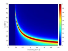
(a) Radiation pattern, $\alpha=30$rad/m

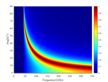
(b) Radiation pattern, $\alpha=60$rad/m

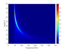
(c) Receive SNR with $\alpha=30$rad/m

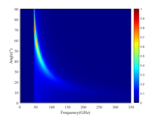
(d) Receive SNR with $\alpha=60$rad/m

Figure 4: Heatmaps to illustrate the leaky-wave antenna’s angle-frequency coupling behaviors in terms of the normalized radiation pattern and receive signal-to-noise ratio (SNR), where $L=5.5$cm, $d=3.5$mm, $q_{t}=-71.76$dBm/Hz, $\sigma_{o}^{2}=-168$dBm/Hz, the free-space path loss model is adopted with a fixed distance $r_{o}=50$m [39, 40].

Since the antenna gain cannot be explicitly calculated, solving the combinatorial problem (13) is challenging. Thus, we provide a low-complexity approach to cope with it. One feature of using leaky-wave antenna is that a large range of THz frequencies (above 0.1 THz) have a nearly identical level of radiation and similar signal strength along a propagation angle, as seen in Fig. 4 (Similar result also seen in Fig. 10 of [14]).

Moreover, the recent THz channel modeling works [39, 40] have demonstrated that given the low range communication distance, pure free-space path loss (FSPL) model can well predict the channel of LoS THz link. It is also shown in Fig. 5 that the molecular absorption loss is relatively marginal for the below 0.35 THz frequency bands, which are the potential 6G frequency bands [3].

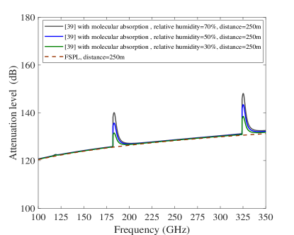
Figure 5: Attenuation levels for the 100GHz-350GHz channels based on the models of [39] and FSPL, respectively. It is seen that FSPL plays a dominant role and the molecular absorption losses with different humidity values are relatively marginal within 250m distance at below 0.35 THz frequency bands.

Therefore, based on FSPL model, constraint $\mathrm{C4}$ in (13) can be rewritten as

$$B_{n}\leq 2f_{n}\frac{{10^{\varepsilon/20}-1}}{{10^{\varepsilon/20}+1}}.$$ (14)

We note that different values of the attenuation coefficient $\alpha$ primarily influence the main-lobe and its nearby side-lobe levels, and have little effect on their trend in the frequency range of interest [18], which is also shown in [34]. Thus we can approximate problem (13) by setting $\alpha=0$. In addition, frequencies of interest need to be close to $f^{\max}\left(\theta\right)$, to achieve large radiated energy. As such, by applying the Taylor series expansion truncated to the first order at $f^{\max}\left(\theta\right)$, $G\left(f,\theta\right)$ with $\alpha=0$ in the frequency range of interest can be evaluated as

$$G\left(f,\theta\right)\approx L-\frac{L^{3}}{24}\left(\beta-k_{0}\cos\theta\right)^{2}.$$ (15)

By considering (14), (15) and $\beta\approx k_{0}\left(1-\frac{f_{\rm co}^{2}}{2f^{2}}\right)$, problem (13) is rewritten as

$$\mathop{\max}\limits_{{\bf{B}},{\bf{f}}}\sum\limits_{n}B_{n}\log_{2}\left(1+F_{\rm SNR}\left(f_{n}\right)\right)$$ (16)

$$\mathrm{s.t.}\leavevmode\nobreak\ \mathrm{C1},\leavevmode\nobreak\ \leavevmode\nobreak\ \mathrm{C2},\leavevmode\nobreak\ \leavevmode\nobreak\ \mathrm{C5},$$

$$\leavevmode\nobreak\ \mathrm{\widetilde{C}3:}\leavevmode\nobreak\ F_{\rm SNR}\left(f_{n}\right)\geq\gamma_{\rm th},\;\,\;\forall n,$$

$$\leavevmode\nobreak\ \mathrm{\widetilde{C}4:}\leavevmode\nobreak\ \eqref{constraint_4},\;\,\;\forall n,$$

where $F_{\rm SNR}\left(f_{n}\right)=\frac{q_{t}\xi\ell\left(r\right)}{\sigma_{o}^{2}}\left(L-\frac{L^{3}k_{0}^{2}}{24}\left(1-\frac{f_{\rm co}^{2}}{2f_{n}^{2}}-\cos\theta\right)^{2}\right)$. To deal with the combinatorial constraint $\mathrm{C2}$, we propose a greedy-based solution. We first find the best $f_{1}^{*}$ by solving the following subproblem

$$\mathop{\max}\limits_{f_{1}}F_{\rm SNR}\left(f_{1}\right)$$ (17)

$$\mathrm{s.t.}\leavevmode\nobreak\ \mathrm{\widetilde{C}3},$$

which means the best center frequency that has the largest signal strength is chosen first. Based on (17), we have

Theorem 1

The optimal solution of the subproblem (17) is given by

$$f_{1}^{*}=\mathbf{1}\left(F_{\rm SNR}\left(f_{1}^{(1)}\right)\geq\gamma_{\rm th}\right)f_{1}^{(1)},$$ (18)

where $f_{1}^{(1)}=\frac{{f_{{\rm{co}}}^{2}}}{{\sqrt{\frac{{12c^{2}}}{{L^{2}\pi^{2}}}+2\left({1-\cos\theta_{o}}\right)f_{{\rm{co}}}^{2}}}}$, and $\mathbf{1}(A)$ represents the indicator function that returns one if the condition $A$ is met.

Proof 1

See Appendix A.

It is shown from Theorem 1 that although the frequency given by (2) has the maximum radiated energy, it may not necessarily achieve the largest signal strength without considering the channel environments. Based on Theorem 1 and problem (16), the optimal bandwidth of the first subchannel with the center frequency $f_{1}^{*}$ is $B_{1}^{*}=2f_{1}^{*}\frac{{10^{\varepsilon/20}-1}}{{10^{\varepsilon/20}+1}}$. As such, we can obtain the center frequency of the $n$-th subchannel and the corresponding subchannel bandwidth as follows:

Theorem 2

The optimal center frequency of the $n$-th ($n\geq 2$) subchannel is given by

$$f_{n}^{*}=\mathbf{1}\left(F_{\rm SNR}\left(f_{n}\right)\geq\gamma_{\rm th}\right)f_{n},$$ (19)

where

$$f_{n}=\left\{\begin{array}[]{l}\Lambda^{-1}f_{\min},\leavevmode\nobreak\ \leavevmode\nobreak\ if\;\hat{F}\left(\Lambda^{-1}f_{\min}\right)>\hat{F}\left(\Lambda f_{\max}\right),\\ \Lambda f_{\max},\quad otherwise,\\ \end{array}\right.$$ (22)

with $\Lambda=10^{\varepsilon/20}$, $f_{\min}=\min\left\{{f_{1}^{*},\cdots,f_{n-1}^{*}}\right\}$, $f_{\max}=\max\left\{{f_{1}^{*},\cdots,f_{n-1}^{*}}\right\}$, and $\hat{F}\left(f\right)=f^{-2}\left(L-\frac{L^{3}\pi^{2}f^{2}}{6c^{2}}\left(1-\frac{f_{\rm co}^{2}}{2f^{2}}-\cos\theta\right)^{2}\right)$. The corresponding subchannel bandwidth is

$$B_{n}^{*}=\min\left\{2f_{n}^{*}\frac{{10^{\varepsilon/20}-1}}{{10^{\varepsilon/20}+1}},{B_{total}-\sum\limits_{b=1}^{n-1}{B_{b}}}\right\},$$ (23)

respectively.

Proof 2

See Appendix B.

Based on Theorem 1 and Theorem 2, we obtain a low-complexity solution of problem (13), which is concluded in Algorithm 1.

Algorithm 1 Solution of Problem (13)

1:  Initialize the number of subchannels $n=1$.

2:  if $n=1$, then

3:     Calculate the center frequency $f_{1}^{*}$ and bandwidth $B_{1}^{*}=2f_{1}^{*}\frac{{10^{\varepsilon/20}-1}}{{10^{\varepsilon/20}+1}}$ of the first subchannel based on Theorem 1.

4:  else

5:     Repeat

6:        $n=n+1$.

7:        Calculate the center frequency $f_{n}^{*}$ and bandwidth $B_{n}^{*}$ of the $n$-th subchannel based on Theorem 2.

8:     Until $B_{n}^{*}=0$.

9:     $N\leftarrow n-1$.

10:  end if Output: Subchannel allocation$\left(f_{n}^{*},B_{n}^{*}\right),n=1,\cdots,N$.

Proposition 1: The proposed Algorithm 1 can achieve the minimum number of subchannels for maximizing the transmission rate under QoS constraint.

Proof 3

Suppose that there is one subchannel $\widetilde{n}$ with the center frequency $f_{\widetilde{n}}$ and bandwidth $B_{\widetilde{n}}$. If the SNR $F_{\rm SNR}\left(f_{\widetilde{n}}\right)<F_{\rm SNR}\left(f_{N}^{*}\right)$ where $f_{N}^{*}$ is the center frequency of the $N$-th subchannel obtained from Algorithm 1, the subchannel $\widetilde{n}$ cannot be added since $N$ subchannels with larger signal strength at center frequencies have already been selected under the total bandwidth constraint; If $F_{\rm SNR}\left(f_{\widetilde{n}}\right)\geq F_{\rm SNR}\left(f_{N}^{*}\right)$, the subchannel $\widetilde{n}$ should be part of one subchannel determined by Algorithm 1. The reason is that under the total bandwidth constraint, there are only $N$ subchannels with different $F_{\rm SNR}\left(f_{n}^{*}\right)(n=1,\cdots,N)$ values that are greater than $F_{\rm SNR}\left(f_{N}^{*}\right)$ and meet $|F_{\rm SNR}\left(f_{n+1}^{*}\right)\sigma_{o}^{2}\left|{{}_{\rm dB}}\right.-F_{\rm SNR}\left(f_{n}^{*}\right)\sigma_{o}^{2}\left|{{}_{\rm dB}}\right.|>\varepsilon$, as indicated in Theorem 1 and Theorem 2. Hence $F_{\rm SNR}\left(f_{\widetilde{n}}\right)$ value should belong to $[F_{\rm SNR}\left(f_{N}^{*}\right),F_{\rm SNR}\left(f_{1}^{*}\right)]$, which completes the proof.

The above subchannel allocation is designed based on the leaky-wave antenna’s radiation pattern and channel quality (namely same transmit PSD value for all the subchannels). As such, the proposed Algorithm 1 provides an efficient approach to select the number of subchannels and their bandwidths for very large THz frequency bands under QoS constraint. In the following section, we proceed to improve the energy efficiency after accomplishing the subchannel allocation.

V Energy Efficiency Enhancement

The prior section has shown that the number of subchannels $N$ and the bandwidth of each subchannel can be easily determined with the help of Algorithm 1. To reduce the power consumption in the THz systems with leaky-wave antennas, we seek to maximize the average EE with respect to the transmit PSDs $\left\{q_{n}\right\}$ of the subchannels. Based on Sections II-IV, the considered problem is formulated as

$$\mathop{\max}\limits_{\bf{q}}\frac{1}{N}\sum\limits_{n=1}^{N}\frac{\log_{2}\left(1+q_{n}\Xi_{n}\right)}{q_{n}+q_{c}}$$ (24)

$$\mathrm{s.t.}\leavevmode\nobreak\ \mathrm{\hat{C}1:}\leavevmode\nobreak\ 0<{q_{n}}\leq q_{\max},\;\,\;\forall n,$$

$$\leavevmode\nobreak\ \leavevmode\nobreak\ \quad\mathrm{\hat{C}2:}\leavevmode\nobreak\ q_{n}\Xi_{n}\geq\gamma_{\rm th},\;\,\;\forall n,$$

where ${\bf{q}}=\left[q_{n}\right]$, $\Xi_{n}=\frac{\widetilde{G}\left(f_{n},\theta\right)\ell\left({r}\right)}{\sigma_{o}^{2}}$, and $q_{c}$ is the PSD due to the hardware’s power consumptions. Constraint $\mathrm{\hat{C}1}$ is the transmit PSD’s feasible range with the maximum value $q_{\max}$, and $\mathrm{\hat{C}2}$ is the QoS constraint. Problem (24) can be decomposed into $N$ subproblems:

$$\mathop{\max}\limits_{q_{n}}\frac{\log_{2}\left(1+q_{n}\Xi_{n}\right)}{q_{n}+q_{c}}$$ (25)

$$\mathrm{s.t.}\leavevmode\nobreak\ \mathrm{\hat{C}1},\leavevmode\nobreak\ \leavevmode\nobreak\ \mathrm{\hat{C}2}.$$

Then, we have the following theorem:

Theorem 3

The optimal transmit PSD of the $n$-th subchannel is given by

$$q_{n}^{*}=\left\{\begin{array}[]{l}q_{\max},\quad if\;\;\widehat{F}_{{\rm{EE}}}\left({q_{\max}}\right)\geq 0,\\ \max\left\{{q_{o},\frac{{\gamma_{\rm th}}}{{\Xi_{n}}}}\right\},\quad otherwise,\\ \end{array}\right.$$ (28)

where $\widehat{F}_{\rm{EE}}\left(q\right)=\frac{q+q_{c}}{1+q\Xi_{n}}\Xi_{n}-\ln\left(1+q\Xi_{n}\right)$, and $q_{o}$ with $\widehat{F}_{\rm{EE}}\left(q_{o}\right)=0$ can be easily obtained by using a one-dimension search in $q_{o}\in\left(0,q_{\max}\right]$ since $\widehat{F}_{\rm{EE}}\left(q\right)$ is a decreasing function.

Proof 4

See Appendix C.

Thus, we obtain a closed-form power allocation solution for enhancing the EE.

VI Simulation Results

This section provides numerical results to validate our analysis and the efficiency of the proposed solution for subchannel allocation and EE enhancement. In the simulations, the transmit PSD is $q_{t}=-71.76$dBm/Hz (namely the total transmit power is 1W in a 15GHz bandwidth), the noise’s PSD is $\sigma_{o}^{2}=-168$dBm/Hz, the inter-plate distance is $d=3.5$mm, $\xi=1$, the free-space path loss model is applied with the LoS path loss exponent $\eta_{\rm LoS}=2$ [39, 40], and the reference distance $D=1$. Based on the 3GPP blockage model [50], the LoS probability function $P_{\rm LoS}\left(r\right)$ with a distance $r$ is given by

$$P_{\rm LoS}\left(r\right)=e^{-r/a_{1}}+\left(1-e^{-r/a_{1}}\right)\min\left(\frac{a_{2}}{r},1\right),$$ (29)

where $a_{1}=63$m and $a_{2}=18$m. The other simulation parameters are detailed in the following simulation results. In addition, the Monte Carlo simulation results are obtained by averaging over $3\times 10^{4}$ trials.

VI-A Average Transmission Rate Analysis

In this subsection, we analyze the effects of different system parameters on the average transmission rate. The analytical results for average transmission rate are obtained from (11).

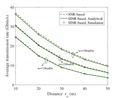
Figure 6: The average transmission rate versus communication distance $r_{o}$ for different $\alpha$ with $\lambda_{\rm THz}=5*10^{-1}$/m², $L=0.06$m, $B_{o}=5$GHz and $f_{o}=270$GHz (namely the LoS direction of the typical receiver is $\theta_{o}=28.7^{o}$ based on (2)).

Fig. 6 shows that our analytical results have a good match with the Monte Carlo simulations for different communication distance and attenuation coefficient values. The use of leaky-wave antenna enables the THz networks to be noise-limited in the presence of highly dense transmitters. In the THz frequencies, slightly increasing the communication distance between a typical transmitter and its receiver can significantly reduce the average transmission rate, due to the higher path loss. In addition, different attenuation coefficients has a negligible effect on the level of interference.

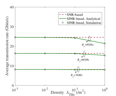
Figure 7: The average transmission rate versus density $\lambda_{\rm{THz}}$ for different subchannel bandwidth $B_{o}$ with $r_{o}=30$m, $L=0.06$m, $\alpha=120$rad/m and $f_{o}=270$GHz(namely $\theta_{o}=28.7^{o}$).

Fig. 7 shows that THz networks with leaky-wave antennas become interference-limited only when extremely dense transmitters (e.g., $\lambda_{\rm THz}=10^{0}$/m² in this figure) utilize large subchannel bandwidth. Moreover, we see that increasing the subchannel bandwidth results in a higher level of interference as $\lambda_{\rm THz}>10^{-1}$/m². The reason is that large subchannel bandwidth corresponds to higher propagation angle difference $\Delta\theta_{o}$ (See (3)), the effects of which are two-fold: 1) More interferers use the same frequency band; 2) The typical receiver is covered by more interferers.

Fig. 8 shows that the average transmission rate significantly decreases in higher center frequencies, due to the fact that spectral efficiency (bits/s/Hz) decreases in higher frequencies with higher path losses under the same radiation pattern. Again, we see that the analytical results match with the Monte Carlo simulations for different values of THz center frequency and aperture length. For higher THz frequencies (e.g., above 300GHz in this figure), the effect of aperture length on the interference is marginal.

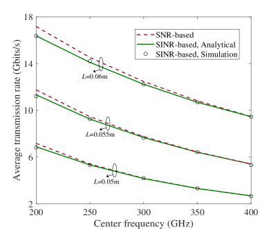
Figure 8: The average transmission rate versus center frequency for different $L$ with $r_{o}=30$m, $\lambda_{\rm THz}=5*10^{-1}$/m², $\alpha=120$rad/m and $B_{o}=5$GHz.

VI-B Subchannel Allocation

In this subsection, we focus on the efficiency of the proposed subchannel allocation solution through comparison with the same number of subchannels with the equal allocation of frequency band. In the simulations, the propagation angle from the transmitter to the receiver is uniformly distributed, i.e., $\theta\in U\left(0,\frac{\pi}{2}\right)$, the communication distance is uniformly distributed within the coverage radius $r_{\max}$, the aperture length $L=0.06$m, $\gamma_{\rm th}=-6.5$dB [51], $\varepsilon=0.2$dB, the continuous broadband spectrum ranging from 100 GHz to 350 GHz is considered, namely $f\in[100,350]$(GHz). The proposed solution is provided based on Algorithm 1, which is in comparison with the equal allocation method (namely equal allocation of frequency band with the same number of subchannels and center frequency given by (2)).

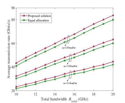
(a) Average transmission rate

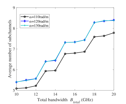
(b) Average number of subchannels

Figure 9: The average transmission rate and number of subchannels versus total bandwidth for different $\alpha$ with the coverage radius $r_{\max}=100$m.

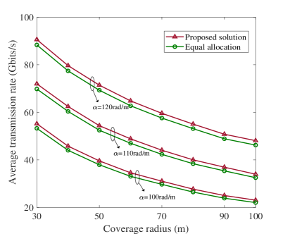
(a) Average transmission rate

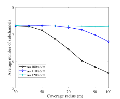
(b) Average number of subchannels

Figure 10: The average transmission rate and number of subchannels versus coverage radius for different $\alpha$ with the total bandwidth $B_{total}=15$GHz.

Fig. 9 shows that the proposed solution outperforms the equal allocation method for different total bandwidths. Slightly increasing the $\alpha$ value leads to the higher average transmission rate when adding the frequency bandwidths. The reason is that based on [18, eq. (7.25)], increasing the $\alpha$ value creates larger beamwidth, which means more frequencies are in the main-lobe that captures large radiated energy. It is seen from Fig. 9(b) that the proposed solution can well control the number of subchannels, e.g., in this figure, the number of subchannels increases by about $60\%$ when doubling the total bandwidth. There exist more subchannels for larger $\alpha$ and total bandwidth, due to the fact that more frequencies in the main-lobe satisfy the QoS constraint and can be applied.

Fig. 10 shows that the proposed solution achieves better performance than the equal allocation method for different coverage areas. When the coverage area of the transmitter is expanded, the performance difference between the far-away receiver and the nearby one is significant, due to the higher path losses in the THz frequencies. An interesting phenomenon is seen in Fig. 10(b), i.e., the average number of subchannels decreases for larger coverage radius and lower attenuation coefficient values. The reason is that lower attenuation coefficient value creates narrower beamwidth, thus more frequencies are in the side-lobes (lower signal strength), which means that more frequencies cannot meet the QoS constraint.

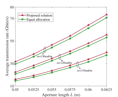
(a) Average transmission rate

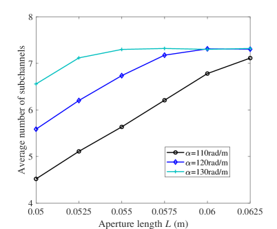
(b) Average number of subchannels

Figure 11: The average transmission rate and number of subchannels versus aperture length for different $\alpha$ with the coverage radius $r_{\max}=100$m and the total bandwidth $B_{total}=15$GHz.

Fig. 11 shows that the proposed solution achieves better performance than the equal allocation method for different aperture lengths. We see that slightly changing the aperture length can have a big impact on the average transmission rate. Such an impact is more significant when increasing the $\alpha$ value. It is indicated from Fig. 11(b) that slightly changing the aperture length also has a big impact on the number of subchannels.

VI-C Energy Efficiency

In this subsection, numerical results are presented by using Theorem 3, and the efficiency of the proposed power allocation solution is confirmed in comparison with the equal power allocation (namely $q_{n}=q_{\max}$, $n=1,\cdots,N$) under the same subchannel allocation obtained by using Algorithm 1. In the simulations, $q_{\max}=-71.76$dBm/Hz, $q_{c}=-81.76$dBm/Hz, the communication distance is uniformly distributed within the coverage radius $r_{\max}=100$m and other basic simulation parameters are the same as those mentioned in subsection VI-B.

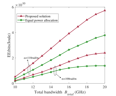
(a) The EE versus total bandwidth for different $\alpha$ with the aperture length $L=0.06$m.

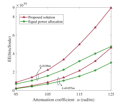
(b) The EE versus attenuation coefficient for different $L$ with the total bandwidth $B_{total}=15$GHz.

Figure 12: Energy efficiency (EE) enhancement.

Fig. 12(a) shows that the proposed solution achieves better EE than the equal power allocation method for different total bandwidths, and the advantage of the proposed solution is more significant when increasing the total bandwidths or $\alpha$ value. The reason is that the increase of the total bandwidths or $\alpha$ value enables more available subchannels (See Fig. 9). The proposed solution can reduce more power consumption. Fig. 12(b) shows that the proposed solution performs better than equal power allocation method for different attenuation coefficients. As mentioned before, the proposed solution saves more energy when increasing the $\alpha$ value. We see that slightly changing the aperture length has a big impact on the EE.

VII Conclusions and Future Work

This paper concentrated on the benefits of using the leaky-wave antenna in the THz networks, where each transmitter leveraged a single leaky-wave antenna to create high antenna gain. We first derived the average transmission rate in the dense THz networks and demonstrated the noise-limited behavior of using the leaky-wave antenna. Our results have shown that the effect of interference becomes significant only when the subchannel bandwidth is large enough and the transmitters are extremely dense. Then, we addressed the subchannel allocation issue for large THz frequency bands, which is crucial for meeting the QoS constraint and tackling the PAPR issue. In light of the leaky-wave antenna’s characteristics, a closed-form solution for subchannel allocation was developed. The results confirmed the efficiency of the proposed subchannel allocation solution compared to the equal allocation method. These results also indicated that the attenuation coefficient of the leaky-wave antenna has a substantial effect on the subchannel allocation. Furthermore, we developed a low-complexity power allocation method for EE enhancement, and the results showed that the proposed method achieves better EE performance than the equal power allocation.

While this work has shown the opportunities of using leaky-wave antennas in large-scale THz networks, more research efforts are required to further evaluate the performance behaviors from different perspectives and develop various transmission designs with leaky-wave antennas. In particular, the spatial-spectral feature of the leaky-wave antenna means that the value of the attenuation coefficient has to be properly designed. The reason is that larger attenuation coefficient values allow more frequencies to be in the main-lobe, which enables higher transmission rate. However, it also brings in more interference for the ultra-dense THz networks. Another area that warrants further research is the transmission design in the scenarios where each transmitter has multiple leaky-wave antennas. In this case, multiplexing gains are more likely to be achieved in the frequency-domain. But it may be hard to achieve large array gains due to the leaky-wave antenna’s spatial-spectral feature, which differs from the beamforming/precoding designs with conventional large arrays in the sub-6 GHz and mmWave frequencies. In addition, further studies are needed for the scenarios such as multi-user transmissions, multi-tier transmissions with sub-6 GHz, mmWave and THz tiers, cognitive radio, wiretap channels, integrated access and backhaul etc.

Appendix A: Proof of Theorem 1

Since $\ell\left(r_{o}\right)=(\frac{{\text{c}}}{{4\pi{f_{1}}}})^{2}\left(\max\left(D,r_{o}\right)\right)^{-\eta}$, problem (16) is equivalently transformed as

$$\mathop{\max}\limits_{f_{1}}\hat{F}\left(f_{1}\right)$$ (A.1)

$$\mathrm{s.t.}\leavevmode\nobreak\ \mathrm{\widetilde{C}3},$$

where

$$\hat{F}\left(f_{1}\right)=f_{1}^{-2}\left(L-\frac{L^{3}\pi^{2}f_{1}^{2}}{6c^{2}}\left(1-\frac{f_{\rm co}^{2}}{2f_{1}^{2}}-\cos\theta\right)^{2}\right).$$ (A.2)

Taking the first-order and second-order derivatives of $\hat{F}\left(f_{1}\right)$ with respect to $f_{1}$ yields

$$\frac{{\partial\hat{F}}}{{\partial f_{1}}}=-{\rm{2}}f_{1}^{-{\rm{3}}}\left({L+\frac{{L^{3}\pi^{2}f_{{\rm{co}}}^{2}}}{{6c^{2}}}\left({1-\frac{{f_{{\rm{co}}}^{2}}}{{2f_{1}^{2}}}-\cos\theta}\right)}\right),$$ (A.3)

and

$${\frac{{\partial^{2}\hat{F}}}{{\partial f_{1}^{2}}}}={\rm{6}}f_{1}^{-4}\left({L+\frac{{L^{3}\pi^{2}f_{{\rm{co}}}^{2}}}{{6c^{2}}}\left({1-\cos\theta}\right)}\right)-{\rm{5}}f_{1}^{-6}\frac{{L^{3}\pi^{2}f_{{\rm{co}}}^{4}}}{{6c^{2}}},$$ (A.4)

respectively. Then, the solutions of $\frac{{\partial\hat{F}}}{{\partial f_{1}}}=0$ and ${\frac{{\partial^{2}\hat{F}}}{{\partial f_{1}^{2}}}}=0$ are given by

$$f_{1}^{(1)}=\frac{{f_{{\rm{co}}}^{2}}}{{\sqrt{\frac{{12c^{2}}}{{L^{2}\pi^{2}}}+2\left({1-\cos\theta}\right)f_{{\rm{co}}}^{2}}}},$$ (A.5)

and

$$f_{1}^{(2)}=\frac{{\sqrt{\rm{5}}f_{{\rm{co}}}^{2}}}{{\sqrt{\frac{{{\rm{36}}c^{2}}}{{L^{2}\pi^{2}}}+6\left({1-\cos\theta}\right)f_{{\rm{co}}}^{2}}}},$$ (A.6)

respectively. According to (A.4) and (A.6), we see that ${\frac{{\partial^{2}\hat{F}}}{{\partial f_{1}^{2}}}}<0$ as $f_{1}\in(0,f_{1}^{(2)})$, and ${\frac{{\partial^{2}\hat{F}}}{{\partial f_{1}^{2}}}}>0$ as $f_{1}\in(f_{1}^{(2)},\infty)$. Since $f_{1}^{(1)}<f_{1}^{(2)}$, we have $\frac{{\partial\hat{F}}}{{\partial f_{1}}}>\frac{{\partial\hat{F}}}{{\partial f_{1}}}|_{f_{1}=f_{1}^{(1)}}=0$ as $f_{1}\in(0,f_{1}^{(1)})$, and $\frac{{\partial\hat{F}}}{{\partial f_{1}}}<0$ as $f_{1}\in(f_{1}^{(1)},\infty)$. Therefore, $f_{1}^{(1)}$ is the optimal solution for maximizing the objective function of problem (A.1). Considering (A.5) and the constraint $\mathrm{C3}$, we obtain Theorem 1.

Appendix B: Proof of Theorem 2

As mentioned in Appendix A, frequencies are selected to maximize the $\hat{F}\left(f\right)$ given by (A.2), and $\hat{F}\left(f\right)$ is the increasing function of $f$ as $f\in(0,f_{1}^{*})$, and the decreasing function of $f$ as $f\in(f_{1}^{*},\infty)$. Let $f_{\min}=\min\left\{{f_{1}^{*},\cdots,f_{n-1}^{*}}\right\}$, if the center frequency $f_{n}$ of the $n$-th subchannel satisfies $f_{n}\in(0,f_{1}^{*})$, it should meet the following condition

$$f_{n}+\frac{B_{n}}{2}=f_{\min}-\frac{B_{\min}}{2},$$ (B.1)

where $B_{\min}$ is the bandwidth of the subchannel with the center frequency $f_{\min}$. Based on (16), we see that $B_{n}=2f_{n}\frac{{10^{\varepsilon/20}-1}}{{10^{\varepsilon/20}+1}}$, and $B_{\min}=2f_{\min}\frac{{10^{\varepsilon/20}-1}}{{10^{\varepsilon/20}+1}}$. Thus, (B.1) is rewritten as

$$f_{n}=10^{-\varepsilon/20}f_{\min}.$$ (B.2)

Likewise, let $f_{\max}=\max\left\{{f_{1}^{*},\cdots,f_{n-1}^{*}}\right\}$, if the center frequency $f_{n}$ of the $n$-th subchannel satisfies $f_{n}\in(f_{1}^{*},\infty)$, we have

$$f_{n}=10^{\varepsilon/20}f_{\max}.$$ (B.3)

Based on (A.1), (B.2) and (B.3), we find that the optimal $f_{n}$ is $10^{-\varepsilon/20}f_{\min}$ when $\hat{F}\left(10^{-\varepsilon/20}f_{\min}\right)>\hat{F}\left(10^{\varepsilon/20}f_{\max}\right)$, otherwise it is $10^{\varepsilon/20}f_{\max}$. As such, we obtain Theorem 2.

Appendix C: Proof of Theorem 3

Let $F_{\rm EE}\left(q_{n}\right)=\frac{1}{\ln 2}\frac{\ln\left({1+q_{n}\Xi_{n}}\right)}{q_{n}+q_{c}}$, which is the objective function of problem (25). Taking the first-order derivative of $F_{\rm EE}$ yields

$$\frac{\partial F_{\rm EE}}{\partial q_{n}}=\frac{1}{\ln 2}\frac{\widehat{F}_{\rm{EE}}\left(q_{n}\right)}{\left({q_{n}+q_{c}}\right)^{2}},$$ (C.1)

where

$$\widehat{F}_{\rm{EE}}\left(q_{n}\right)=\frac{q_{n}+q_{c}}{1+q_{n}\Xi_{n}}\Xi_{n}-\ln\left(1+q_{n}\Xi_{n}\right).$$ (C.2)

Since $\frac{{\partial\widehat{F}_{{\rm{EE}}}}}{{\partial q_{n}}}=-\frac{{\left({q_{c}+q_{n}}\right)\Xi_{n}^{2}}}{{\left({1+q_{n}\Xi_{n}}\right)^{2}}}<0$, $\widehat{F}_{\rm{EE}}\left(q_{n}\right)$ is a decreasing function of $q_{n}$. Based on the constraints $\mathrm{\hat{C}1}$ and $\mathrm{\hat{C}2}$, we see that $\frac{\gamma_{\rm th}}{\Xi_{n}}<q_{n}<q_{\max}$. Then, two cases need to be considered as follows:

• Case 1: When $\widehat{F}_{\rm{EE}}\left(q_{\max}\right)\geq 0$, $\widehat{F}_{\rm{EE}}\left(q_{n}\right)>0$ and thus $\frac{\partial F_{\rm EE}}{\partial q_{n}}>0$ for $q_{n}\in\left(\frac{\gamma_{\rm th}}{\Xi_{n}},q_{\max}\right]$, i.e., $F_{\rm EE}\left(q_{n}\right)$ is an increasing function of $q_{n}$, hence the optimal $q_{n}^{*}$ is $q_{n}^{*}=q_{\max}$.

• Case 2: When $\widehat{F}_{\rm{EE}}\left(q_{\max}\right)<0$, $q_{o}$ with $\widehat{F}_{\rm{EE}}\left(q_{o}\right)=0$ can be easily obtained by using a one-dimension search for $q_{o}\in\left(0,q_{\max}\right]$. Then, we see that $\frac{\partial F_{\rm EE}}{\partial q_{n}}\geq 0$ for $q_{n}\in\left(0,q_{o}\right]$ and $\frac{\partial F_{\rm EE}}{\partial q_{n}}<0$ for $q_{n}\in\left(q_{o},q_{\max}\right]$. Therefore, $q_{n}^{*}=\max\left\{q_{o},\frac{\gamma_{\rm th}}{\Xi_{n}}\right\}$ is the optimal solution.

As such, we get the optimal $q_{n}^{*}$ given in Theorem 3.

References

- [1] 3GPP TS 38.104 v16.4.0, “NR; Base Station (BS) radio transmission and reception (Release 16),” June 2020.
- [2] S. Koenig et al., “Wireless sub-THz communication system with high data rate,” Nature Photonics, vol. 7, pp. 977–981, Dec. 2013.
- [3] T. S. Rappaport et al., “Wireless communications and applications above 100 GHz: Opportunities and challenges for 6G and beyond,” IEEE Access, vol. 7, pp. 78 729–78 757, June 2019.
- [4] K. Rikkinen, P. Kyöti, M. E. Leinonen, M. Berg, and A. Pärssinen, “THz radio communication: Link budget analysis toward 6G,” IEEE Commun. Mag., vol. 58, no. 11, pp. 22–27, Nov. 2020.
- [5] S. Sun, T. S. Rappaport, R. W. Heath, Jr., A. Nix, and S. Rangan, “MIMO for millimeter-wave wireless communications: Beamforming, spatial multiplexing, or both?” IEEE Commun. Mag., vol. 7, no. 12, pp. 110–121, Dec. 2014.
- [6] O. E. Ayach, S. Rajagopal, S. Abu-Surra, Z. Pi, and R. W. Heath, Jr., “Spatially sparse precoding in millimeter wave MIMO systems,” IEEE Trans. Wireless Commun., vol. 13, no. 3, pp. 1499–1513, Mar. 2014.
- [7] C. Lin and G. Y. Li, “Energy-efficient design of indoor mmWave and Sub-THz systems with antenna arrays,” IEEE Trans. Wireless Commun., vol. 15, no. 7, pp. 4660–4672, July 2016.
- [8] Z. Chen, X. Ma, B. Zhang, Y. Zhang, Z. Niu, N. Kuang, W. Chen, L. Li, and S. Li, “A survey on terahertz communications,” China Commun., vol. 16, no. 2, pp. 1–35, Feb. 2019.
- [9] B. Peng, S. Wesemann, K. Guan, W. Templ, and T. Kürner, “Precoding and detection for broadband single carrier terahertz massive MIMO systems using LSQR algorithm,” IEEE Trans. Wireless Commun., vol. 18, no. 2, pp. 1026–1040, Feb. 2019.
- [10] L. You, X. Chen, X. Song, F. Jiang, W. Wang, X. Gao, and G. Fettweis, “Network massive MIMO transmission over millimeter-wave and terahertz bands: Mobility enhancement and blockage mitigation,” IEEE J. Sel. Areas Commun., vol. 38, no. 12, pp. 2946–2960, Dec. 2020.
- [11] L. Yan, C. Han, and J. Yuan, “A dynamic array-of-subarrays architecture and hybrid precoding algorithms for terahertz wireless communications,” IEEE J. Sel. Areas Commun., vol. 38, no. 9, pp. 2041–2056, Sept. 2020.
- [12] X. Fu, F. Yang, C. Liu, X. Wu, and T. J. Cui, “Terahertz beam steering technologies: From phased arrays to field-programmable metasurfaces,” Adv. Opt. Mater., vol. 8, no. 3, pp. 1–22, Feb. 2020.
- [13] G. Zhang, Q. Zhang, Y. Chen, T. Guo, C. Caloz, and R. D. Murch, “Dispersive feeding network for arbitrary frequency beam scanning in array antennas,” IEEE Trans. Antennas Propag., vol. 65, no. 6, pp. 3033–3040, June 2017.
- [14] Y. Ghasempour, C. Yeh, R. Shrestha, D. Mittleman, and E. Knightly, “Single shot single antenna path discovery in THz networks,” in Proc. 26th MobiCom, 2020, pp. 1–13.
- [15] D. Headland, Y. Monnai, D. Abbott, C. Fumeaux, and W. Withayachumnankul, “Tutorial: Terahertz beamforming, from concepts to realizations,” APL Photonics, vol. 3, no. 5, pp. 1–32, 2018.
- [16] I. Frigyes and A. J. Seeds, “Optically generated true-time delay in phased-array antennas,” IEEE Trans. Microw. Theory Techn., vol. 43, no. 9, pp. 2378–2386, Sept. 1995.
- [17] A. A. Oliner and D. R. Jackson, “Leaky-wave antennas,” in Antenna Engineering Handbook, J. L. Volakis, Ed. New York: McGraw-Hill,2007.
- [18] D. R. Jackson and A. A. Oliner, “Leaky-wave antennas,” in Modern Antenna Handbook, C. Balanis, Ed. New York: Wiley, 2008.
- [19] D. R. Jackson, C. Caloz, and T. Itoh, “Leaky-wave antennas,” Proc. IEEE, vol. 100, no. 7, pp. 2194–2206, July 2012.
- [20] I. Bahl and K. Gupta, “Frequency scanning by leaky-wave antennas using artificial dielectrics,” IEEE Trans. Antennas Propag., vol. 23, no. 4, pp. 584–589, July 1975.
- [21] G. Zhang, Q. Zhang, S. Ge, Y. Chen, and R. D. Murch, “High scanning-rate leaky-wave antenna using complementary microstrip-slot stubs,” IEEE Trans. Antennas Propag., vol. 67, no. 5, pp. 2913–2922, May 2019.
- [22] N. J. Karl, R. W. McKinney, Y. Monnai, R. Mendis, and D. M. Mittleman, “Frequency-division multiplexing in the terahertz range using a leaky-wave antenna,” Nature Photonics, vol. 9, pp. 717–721, Sept. 2015.
- [23] K. Murano, I. Watanabe, A. Kasamatsu, S. Suzuki, M. Asada, W. Withayachumnankul, T. Tanaka, and Y. Monnai, “Low-profile terahertz radar based on broadband leaky-wave beam steering,” IEEE Trans. Terahertz Sci. Technol., vol. 7, no. 1, pp. 60–69, Jan. 2017.
- [24] Y. Amarasinghe, R. Mendis, and D. M. Mittleman, “Real-time object tracking using a leaky THz waveguide,” Opt. Express, vol. 28, no. 12, pp. 17 997–18 005, June 2020.
- [25] H. Matsumoto, I. Watanabe, A. Kasamatsu, and Y. Monnai, “Integrated terahertz radar based on leaky-wave coherence tomography,” Nature Electronics, vol. 3, pp. 122–129, Feb. 2020.
- [26] C.-Y. Yeh, Y. Ghasempour, Y. Amarasinghe, D. M. Mittleman, and E. W. Knightly, “Security in terahertz WLANs with leaky wave antennas,” in ACM WiSec, 2020, pp. 1–11.
- [27] M. Polese, J. M. Jornet, T. Melodia, and M. Zorzi, “Toward end-to-end, full-stack 6G terahertz networks,” IEEE Commun. Mag., vol. 58, no. 11, pp. 48–54, Nov. 2020.
- [28] Y. Ghasempour, C. Yeh, R. Shrestha, Y. Amarasinghe, D. Mittleman, and E. Knightly, “LeakyTrack: Non-coherent single-antenna nodal and environmental mobility tracking with a leaky-wave antenna,” in Proc. 18th SenSys, 2020, pp. 1–13.
- [29] T. S. Rappaport, G. R. MacCartney, Jr., M. K. Samimi, and S. Sun, “Wideband millimeter-wave propagation measurements and channel models for future wireless communication system design,” IEEE Trans. Commun., vol. 63, no. 9, pp. 3029–3056, Sept. 2015.
- [30] N. Khalid and O. B. Akan, “Wideband THz communication channel measurements for 5G indoor wireless networks,” in Proc. IEEE Int. Conf. Commun. (ICC), May 2016, pp. 1–6.
- [31] J. Ma, R. Shrestha, L. Moeller, and D. M. Mittleman, “Channel performance of indoor and outdoor terahertz wireless links,” APL Photonics, vol. 3, no. 5, 1-8, 2018.
- [32] T. Bai and R. W. Heath, Jr., “Coverage and rate analysis for millimeter-wave cellular networks,” IEEE Trans. Wireless Commun., vol. 14, no. 2, pp. 1100–1114, Feb. 2015.
- [33] M. Haenggi, J. G. Andrews, F. Baccelli, O. Dousse, and M. Franceschetti, “Stochastic geometry and random graphs for the analysis and design of wireless networks,” IEEE J. Sel. Areas Commun., vol. 27, no. 7, pp. 1029–1046, Sept. 2009.
- [34] A. Sutinjo, M. Okoniewski, and R. H. Johnston, “Radiation from fast and slow traveling waves,” IEEE Antennas Propag. Mag., vol. 50, no. 4, pp. 175–181, Aug. 2008.
- [35] R. Mendis and D. M. Mittleman, “A 2-D artificial dielectric with for the terahertz region,” IEEE Trans. Microw. Theory Techn., vol. 58, no. 7, pp. 1993–1998, July 2010.
- [36] J. G. Andrews, T. Bai, M. N. Kulkarni, A. Alkhateeb, A. K. Gupta, and R. W. Heath, Jr., “Modeling and analyzing millimeter wave cellular systems,” IEEE Trans. Commun., vol. 65, no. 1, pp. 403–430, Jan. 2017.
- [37] T. S. Rappaport, S. Sun, R. Mayzus, H. Zhao, Y. Azar, K. Wang, G. N. Wong, J. K. Schulz, M. Samimi, and F. Gutierrez, “Millimeter wave mobile communications for 5G cellular: It will work!” IEEE Access, vol. 1, pp. 335–349, 2013.
- [38] X. Yu, J. Zhang, M. Haenggi, and K. B. Letaief, “Coverage analysis for millimeter wave networks: The impact of directional antenna arrays,” IEEE J. Sel. Areas Commun., vol. 35, no. 7, pp. 1498–1512, July 2017.
- [39] J. Kokkoniemi, J. Lehtomäki, and M. Juntti, “Simple molecular absorption loss model for 200-450 gigahertz frequency band,” in Proc. European Conf. Netw. Commun. (EuCNC), 2019, pp. 219–223.
- [40] J. Kokkoniemi, J. Lehtomäki, and M. Juntti, “A line-of-sight channel model for the 100-450 gigahertz frequency band,” EURASIP J. Wireless Com Network, pp. 1–15, Apr. 2021.
- [41] M. K. Samimi et al., “28 GHz angle of arrival and angle of departure analysis for outdoor cellular communications using steerable beam antennas in New York City,” in Proc. IEEE VTC, Jun. 2013, pp. 1–6.
- [42] K. A. Hamdi, “Capacity of MRC on correlated Rician fading channels,” IEEE Trans. Commun., vol. 56, no. 5, pp. 708–711, May 2008.
- [43] Y. Zhu, L. Wang, K.-K. Wong, and R. W. Heath, Jr., “Secure communications in millimeter wave ad hoc networks,” IEEE Trans. Wireless Commun., vol. 16, no. 5, pp. 3205–3217, May 2017.
- [44] S. H. Han and J. H. Lee, “An overview of peak-to-average power ratio reduction techniques for multicarrier transmission,” IEEE Wireless Commun., vol. 12, no. 2, pp. 56–65, Apr. 2005.
- [45] G. Yu, S. He, D. Yu, L. Yang, , and G. Zuo, “An efficient low PAPR training sequence design scheme under spectral constraints in mm-Wave OFDM communication,” in Int. Conf. Wireless Commun. Signal Process. (WCSP), 2015, pp. 1–5.
- [46] S. Shakib, M. Elkholy, J. Dunworth, V. Aparin, and K. Entesari, “A wideband 28GHz power amplifier supporting 8100MHz carrier aggregation for 5G in 40nm CMOS,” in IEEE Int. Solid-state Cricuits Conf. (ISSCC), 2017, pp. 44–46.
- [47] F. Wang, T.-W. Li, and H. Wang, “A highly linear super-resolution mixed-signal doherty power amplifier for high-efficiency mm-Wave 5G Multi-Gb/s communications,” in IEEE Int. Solid-state Cricuits Conf. (ISSCC), 2019, pp. 88–90.
- [48] T. Chi, M.-Y. Huang, S. Li, and H. Wang, “A packaged 90-to-300GHz transmitter and 115-to-325GHz coherent receiver in CMOS for full-band continuous-wave mm-Wave hyperspectral imaging,” in IEEE Int. Solid-state Cricuits Conf. (ISSCC), 2017, pp. 304–305.
- [49] P. Sen, V. Ariyarathna, A. Madanayake, and J. M. Jornet, “Experimental wireless testbed for ultrabroadband terahertz networks,” in ACM WiNTECH, 2020, pp. 48–55.
- [50] 3GPP TR 36.814, “Further Advancements for E-UTRA Physical Layer Aspects (Release 9),” Mar. 2010.
- [51] S. H. A. Shah, S. Aditya, S. Dutta, C. Slezak, and S. Rangan, “Power efficient discontinuous reception in THz and mmWave wireless systems,” in IEEE SPAWC, 2019, pp. 1–5.