Three isotopologues CO survey of Molecular Clouds in the CMa OB1 complex

Abstract

Using the Purple Mountain Observatory 13.7-m millimeter telescope at Delingha in China, we have conducted a large-scale simultaneous survey of ¹²CO, ¹³CO, and C¹⁸O ($J$ = 1–0) toward the CMa OB1 complex with a sky coverage of 16.5 deg² ($221\fdg 5\leq l\leq 227\arcdeg$, $-2\fdg 5\leq b\leq 0\fdg 5$). Emission from the CMa OB1 complex is found in the range 7 km s${}^{-1}\ \leq$ V${}_{\mathrm{LSR}}\ \leq$ 25 km s^-1. The large-scale structure, physical properties and chemical abundances of the molecular clouds are presented. A total of 83 C¹⁸O molecular clumps are identified with GaussClumps algorithm within the mapped region. We find that 94% of these C¹⁸O molecular clumps are gravitationally bound. The relationship between their size and mass indicates that none of the C¹⁸O clump has the potential to form high-mass stars. Using semi-automatic IDL algorithm, we newly discover 85 CO outflow candidates in the mapped area, including 23 bipolar outflows candidates. Additionally, a comparative study reveals evidence for significant variety of physical properties, evolutionary stages, and levels of star formation activity in different sub-regions of the CMa OB1 complex.



1 Introduction

The CMa OB1 complex is a frequently studied and relatively nearby star-forming region in the third Galactic quadrant. A rich collection of objects lies in this region, including more than 30 nebulae (Herbst et al., 1978), two Hii regions (Sharpless, 1959), three water masers (Brand et al., 1994), as well as a large number of young stellar objects (YSOs; Elia et al., 2013; Sewiło et al., 2019).

Many achievements have been made in previous CO surveys toward the CMa OB1 complex. Blitz (1980) first observed and studied CO molecules in this region, although their resolution was only 8.8$\arcmin$. Blitz (1980) revealed molecular emission arising from two distinct clouds, which appeared to be associated with the Hii region $S$292 and $S$296. Later, Kim et al. (2004) made large-scale observation of ¹³CO ($J$ = 1–0) line in this region using the NANTEN 4-m telescope at 2.6$\arcmin$ resolution. They detected three massive star-forming ¹³CO clouds and six intermediate- or low-mass ¹³CO clouds within the CMa OB1 complex. The same telescope was used to map the CMa OB1 complex using the ¹²CO ($J$ = 1–0) line (Elia et al., 2013). Elia et al. (2013) revealed that 93% “¹²CO clumps” are sub-virial, and they obtained a power-law fit to high-mass portion of the “¹²CO clumps” distribution, $N(\log M)\propto M^{\alpha}$, which had a power-law index of $-0.7\pm 0.3$. More recent large-scale ¹²CO and ¹³CO observations of the CMa OB1 complex were made with the ARO 12-m antenna (Benedettini et al., 2020). Although conducted with improved spatial resolution, the root mean square (RMS) noise levels of the ARO survey were 0.79–1.31 K (for ¹²CO), and 0.33–0.58 K (for ¹³CO), with a velocity resolution of 0.65 km s^-1. To date, C¹⁸O observation has been conducted toward the $l$=224$\arcdeg$ field (with sky coverage of about 200 arcmin²; Olmi et al., 2016), using the Mopra radio telescope.

However, limited by their relatively low spatial resolution, and/or sensitivity, to date no unbiased molecular outflow survey has been carried out towards the CMa OB1 complex. In addition, there is a lack of large-scale C¹⁸O observations toward the CMa OB1 complex, which is generally optically thin and therefore allows us to probe the interior of molecular clouds (MCs) therein.

In this paper, we present a new $J$ = 1–0 ¹²CO/¹³CO/C¹⁸O survey towards the CMa OB1 complex with a sky coverage of 16.5 deg² ($221\fdg 5\leq l\leq 227\arcdeg$, $-2\fdg 5\leq b\leq 0\fdg 5$), which is part of the ongoing project Milky Way Imaging Scroll Painting (MWISP; refer to Zhang et al., 2014; Sun et al., 2015; Du et al., 2017; Sun et al., 2017; Su et al., 2019, etc., for project details and initial results). This set of ¹²CO and ¹³CO data, which has a high spatial resolution, high velocity resolution, and high sensitivity have allowed us to carry out the first unbiased search for molecular outflows in this region. Besides, this is the first time the CMa OB1 complex has been observed at a large-scale with C¹⁸O line, which allowed us to carry out the first search for dense molecular clumps that are related to star formation.

The remainder of this paper is organized as follows. In Section 2, we describe the data quality of the CMa OB1 complex. The large-scale structure, physical properties and chemical abundances of the MCs are presented in Section 3. Next, in Section 4, we identify the C¹⁸O clumps and analyze their physical properties. In Section 5, we search for CO molecular outflow candidates and investigate their physical properties. In Section 6, we discuss the analysis of the physical association between the compact C¹⁸O clumps and the outflow candidates. Finally, in Section 7 a summary of our results is given.

2 Data

The observations used in this study were conducted during September 2017 to April 2018 using the 13.7-m millimeter-wavelength telescope of the Purple Mountain Observatory (PMO) in Delingha, China. Using the nine-beam superconducting spectroscopic array receiver (SSAR), working in sideband separation mode and employing the fast Fourier transform spectrometer (FFTS) (Shan et al., 2012), the lines of three CO isotopologues (¹²CO, ¹³CO, and C¹⁸O ($J$ = 1–0)) were observed simultaneously. The ¹²CO line was observed at the upper sideband (USB) with a main-beam width of $\sim$ 48$\arcsec$, and the ¹³CO and C¹⁸O lines were observed at the lower sideband (LSB) with a main-beam width of $\sim$ 50$\arcsec$. Both bandwidths were 1000 MHz with 16,384 channels, resulting in velocity separations of about 0.159 km s^-1for ¹²CO and 0.166 km s^-1for ¹³CO and C¹⁸O. The typical noise temperatures including the atmosphere at 110 GHz and 115 GHz are 140 K and 250 K, respectively. A detailed description of the instrument was given by Shan et al. (2012). All observations were conducted by using position-switch On-The-Fly (OTF) mode.

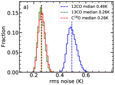
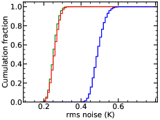
Figure 1: ($a$) Histograms of the rms noise levels ($\sigma$) for ¹²CO (blue), ¹³CO (green), and C¹⁸O (red). ($b$) Cumulative distributions of $\sigma$.

A first-order baseline was applied to the spectra in this study. All the data were sampled every 30$\arcsec$. The RMS distributions are presented in Figure 1. The typical RMS noise levels of the spectra are 0.49 K for ¹²CO ($J$ = 1–0) at a velocity resolution of 0.159 km s^-1, and 0.26 K for ¹³CO ($J$ = 1–0) and C¹⁸O ($J$ = 1–0) at 0.166 km s^-1. Please also refer to Su et al. (2019) for the detailed observations and data-reduction strategies. The velocity channels were re-gridded into 0.168 km s^-1in this study, which facilitated comparisons between the channel-by-channel emission from the three CO lines.

3 Large-scale Molecular Clouds

3.1 Molecular Gas Distributions

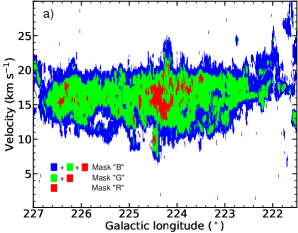
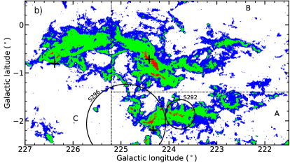
Figure 2: ($a$) Longitude–velocity map, integrated over Galactic latitudes $b$ = $-2\fdg 5$ to $0\fdg 5$. ($b$) Longitude-latitude map, integrated over velocities $V_{\rm LSR}$ = 0 to 30 km s^-1. The crosses represent of positions of the three known water masers (Brand et al., 1994). The two known Hii regions from Sharpless (1959) are also shown as circles. The blue, green and red colors in both maps indicate the mask regions with detectable ¹²CO, ¹³CO, and C¹⁸O emission, respectively, as described in §3.1.

Figure 2 presents longitude-velocity ($l$-$v$) and longitude-latitude ($l$-$b$) maps of all three CO isotopologue emission lines in the CMa OB1 complex, which were obtained by integrating the emission over Galactic latitude $b$ = $-2\fdg 5$ to $0\fdg 5$, and local standard of rest (LSR) velocity $V_{\rm LSR}$ = 0 to 30 km s^-1, respectively. To reduce the influence of noise, the ¹²CO, ¹³CO, and C¹⁸O data were integrated over all channels which had at least three contiguous channels above 3$\sigma$ (i.e., $\gtrsim$ 1.5 K for ¹²CO, and $\gtrsim$ 0.75 K for ¹³CO and C¹⁸O). Similar to Sun et al. (2020), we define mask “B” as the region where ¹²CO emission existed, mask “G” as the region where ¹²CO and ¹³CO emission were detected, and mask “R” as the region where ¹²CO, ¹³CO, and C¹⁸O emission were simultaneously present.

The CMa OB1 complex is concentrated within the $V_{\rm LSR}$ range of 7 to 25 km s^-1, and is located in the Local arm. The main part of the CMa OB1 complex appears as a single, merged structure, as detected via ¹²CO emission, while it shows many fragmented and discontinuous structures via ¹³CO emission Base on the morphology of ¹³CO emission, we roughly divided the CMa OB1 complex into three sub-regions, as shown in Figure 2 (i.e., sub-regions A, B, and C). Each sub-region contains an extended structure with an angular area larger than 1500 arcmin², which corresponds to the three most massive ¹³CO clouds 3 (sub-region A), 4 (sub-region B), and 12 (sub-region C) of Kim et al. (2004), respectively. Coincidently, each sub-region resides one known water maser (Brand et al., 1994), which are indicated as crosses in Figure 2. The two known connected Hii regions $S$292 and $S$296 are also shown in the Figure 2, which are marked as circles (Sharpless, 1959).

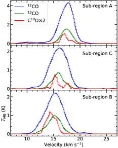
Figure 3: Averaged spectra of ¹²CO (blue), ¹³CO (green), and C¹⁸O (red) for each region. Note that only those spectra with at least three contiguous channels $\gtrsim$ 3$\sigma$ are averaged.

The averaged spectra of ¹²CO (blue), ¹³CO (green), and C¹⁸O (red) for each sub-region are shown in Figure 3. Obviously, the total integrated intensity, LSR velocity, and line width of each sub-region for each isotopologue is different; these values are summarized in Table 1. The LSR velocity of sub-region A is apparently different from the other two sub-regions, which may be due to the feedback from Hii region. The C¹⁸O line profile of sub-region C seems to exhibit two velocity components (one at $\sim$15.5 km s^-1, and another at $\sim$17.5 km s^-1). The full-width half-maximum (FWHM) line width is the largest in sub-region B, while it is the smallest in sub-region A. Generally, the results revealed from our new ¹³CO data are consistent with those of Kim et al. (2004).

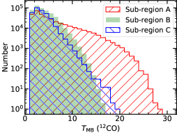
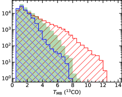
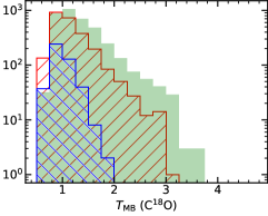
Figure 4: Histograms of the main-beam temperatures of the ¹²CO, ¹³CO, and C¹⁸O emission for each region. Note that only voxels with at least three continuous channels above 3$\sigma$ are plotted.

Figure 4 presents the distributions of $T_{\mathrm{MB}}$ of the three sub-regions for each isotopologue. Note that only those voxels with at least three continuous channels above 3$\sigma$ are plotted. We can see that sub-region A dominates the high value wing of the $T_{\rm MB}$(¹²CO) and $T_{\rm MB}$(¹³CO), yet shows weaker C¹⁸O emission than sub-region B. Instead, sub-region B exhibits the strongest C¹⁸O emission, and the weakest ¹²CO emission. All these results could be interpreted as the different evolutionary stages of star formation for sub-regions A, B, and C, which will be discussed in detail in §3.3.

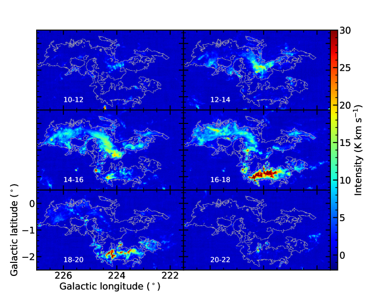
Figure 5: Velocity channel maps of ¹²CO emission in the CMa OB1 complex. The gray contour indicates the boundary of the largest ¹²CO Mc, which was defined as an independent consecutive structure in $l$–$b$ space in Figure 2(b). Each map was integrated over a velocity interval of 2 km s^-1, and the velocity ranges are marked in each panel.

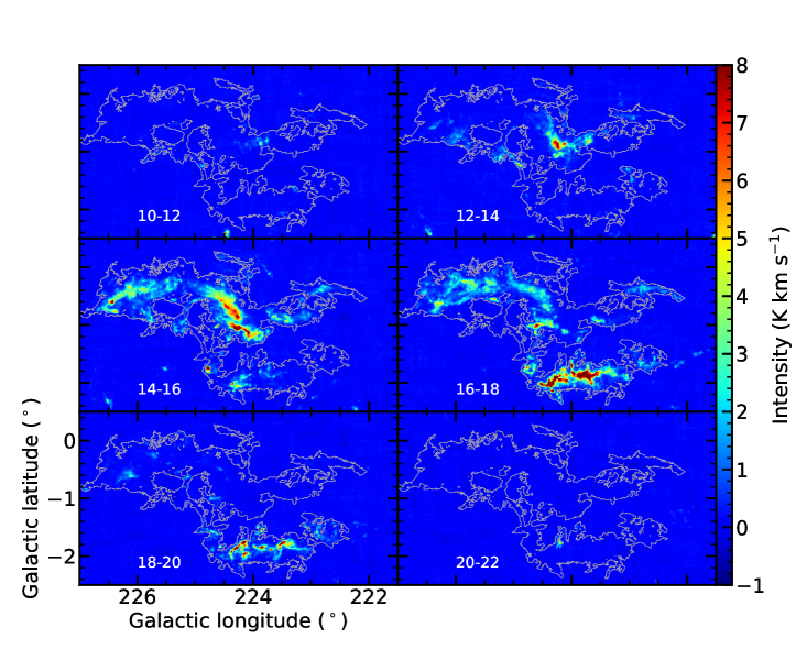
Figure 6: Same as Fig. 5, but for ¹³CO emission.

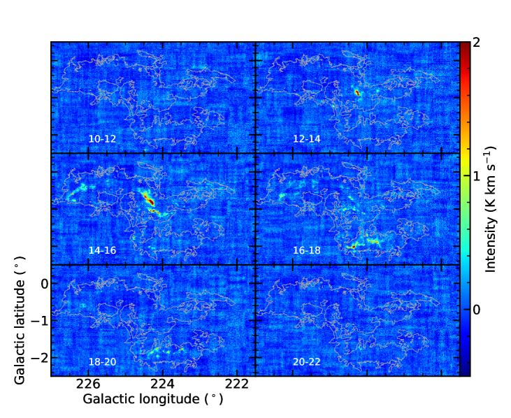
Figure 7: Same as Fig. 5, but for C¹⁸O emission.

Figures 5–7 present the channel maps of ¹²CO, ¹³CO, and C¹⁸O lines, respectively. Interestingly, the molecular gas emission is characterized by filamentary structures, especially in the denser gas traced by ¹³CO and C¹⁸O emission. The filamentary structures in the major parts of the mapped region have been studied by using $Herschel$ data (Sewiło et al., 2019). These molecular line data with additional velocity information, might be helpful for identifying the velocity-coherent filaments, but this theme seems beyond the scope of this study.

3.2 Physical Properties of Molecular Cloud

The distance to the CMa OB1 complex has been measured by various methods. Using photometric observations of OB stars in the CMa OB1 complex, Clariá (1974) determined a distance of 1150$\pm$140 pc for the association. Later, a physical connection between the OB association and the MCs in the CMa OB1 was confirmed (e.g., Machnik et al., 1980; Blitz, 1980). NANTEN CO(1-0) observations were used to derive the kinematic distances of “¹²CO clumps” in the CMa OB1 complex, which were constrained to a range of 800 to 1000 pc (Elia et al., 2013). Considering the much higher accuracy of the photometric method, we adopt a value of 1150 pc as the distance to the CMa OB1 complex.

Using the equations $I(\mathrm{CO})_{i,j}\ =\ \int{T_{\mathrm{MB}}dv}$ and $I(\mathrm{CO})\ =\ a^{2}\sum\limits_{i,j}{I(\mathrm{CO})_{i,j}}$, where $a$ (equal to 30$\arcsec$) is the angular size of each pixel, we estimate the total integrated intensities and areas of the emission of all three CO isotopologues (see Table 1). The total integrated intensities of ¹²CO, ¹³CO, and C¹⁸O emission were found to be $2.1\times 10^{5}$, $2.5\times 10^{4}$, and $3.5\times 10^{2}$ K km s^-1 arcmin², within the three mask areas (i.e., mask “B”, “G”, “R”) in Figure 2(b).

In this study, the properties of the molecular gas were estimated under the assumption that all the molecular gas is in local thermodynamic equilibrium (LTE). We assume that ¹²CO emission is optically thick. Based on these, the excitation temperature ($T_{\mathrm{ex}}$) can be estimated by (Nagahama et al., 1998),

$$T_{\mathrm{ex}}=\frac{5.53}{\ln\left(1+\frac{5.53}{T_{\mathrm{MB,12}}}\right)},$$ (1)

where $T_{\mathrm{MB,12}}$ is the peak main beam temperature of ¹²CO. Assuming that different isotopologues have the same $T_{\mathrm{ex}}$, the optical depths of ¹³CO ($\tau_{13}$), and C¹⁸O ($\tau_{18}$) were estimated as (Kawamura et al., 1998; Pineda et al., 2010):

$$\tau_{13}=-\ln\left\{1-\frac{T_{\mathrm{MB,13}}}{5.29}[(e^{5.29/T_{\mathrm{ex}}}-1)^{-1}-0.164]^{-1}\right\},$$ (2)

$$\tau_{18}=-\ln\left\{1-\frac{T_{\mathrm{MB,18}}}{5.27}[(e^{5.27/T_{\mathrm{ex}}}-1)^{-1}-0.166]^{-1}\right\},$$ (3)

where $T_{\mathrm{MB,13}}$ and $T_{\mathrm{MB,18}}$ are the peak main beam temperatures of ¹³CO and C¹⁸O, respectively. Considering the correction factor for an optical depth of $f=\frac{\tau}{1-e^{-\tau}}$ (Li et al., 2015), the total integrated intensities of ¹³CO and C¹⁸O after optical depth correction can be estimated as:

$$I_{13}=\frac{\tau_{13}}{1-e^{-\tau_{13}}}\times\frac{1+0.88/T_{\mathrm{ex}}}{1-e^{-5.29/T_{\mathrm{ex}}}}\int{T_{\mathrm{MB,13}}dv},$$ (4)

$$I_{18}=\frac{\tau_{18}}{1-e^{-\tau_{18}}}\times\frac{1+0.88/T_{\mathrm{ex}}}{1-e^{-5.27/T_{\mathrm{ex}}}}\int{T_{\mathrm{MB,18}}dv}.$$ (5)

The column densities of ¹³CO and C¹⁸O were estimated as $N_{13}=2.42\times 10^{14}I_{13}$, and $N_{18}=2.54\times 10^{14}I_{18}$ (Garden et al., 1991; Bourke et al., 1997). The isotopic ratios of [¹²C/¹³C] = 77, [¹⁶O/¹⁸O] = 560 (Wilson, & Rood, 1994), and [H₂/¹²CO ] abundance ratio of 1.1$\times 10^{5}$ (Frerking et al., 1982) were used to derive H₂ column density.

The H₂ column densities traced by ¹²CO can be estimated by adopting a CO-to-H₂ conversion factor ($X_{\mathrm{CO}}$ $\equiv$ $N_{\rm H_{2}}$/$I_{\mathrm{CO}}$). Using ¹²CO and ¹³CO data, Barnes et al. (2015, 2018) first examined the relation between the $I_{\mathrm{CO}}$ and $X_{\mathrm{CO}}$ = $N_{\rm H_{2}}$/$I_{\mathrm{CO}}$ (where $N_{\rm H_{2}}$ is derived from ¹³CO). They calculated the $X_{\mathrm{CO}}$ factor in both 3D data cubes and 2D images from all channels and pixels where both ¹²CO and ¹³CO are detected. Using MWISP ¹²CO and ¹³CO data, Sun et al. (2020) derived $X_{\mathrm{CO}}$ for a $\sim$110 deg² region in the Galactic coordinate range of $l$=[129$\fdg$75, 140$\fdg$25] and $b$=[$-$5$\fdg$25, +5$\fdg$25] (hereafter the G130 region). All of these studies confirmed that $X_{\mathrm{CO}}$ varies from region to region. Therefore, following their analytical approach, we derived the $X_{\mathrm{CO}}$ for all locations that had both ¹²CO and ¹³CO detections (mask ‘G’ region), then applied $X_{\mathrm{CO}}$ to locations that had ¹²CO detections (mask ‘B’ region) to the calculated column densities.

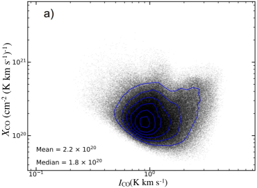
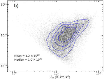
Figure 8: Relations between $N_{\mathrm{H_{2}}}$/$I_{CO}$ and $I_{\mathrm{CO}}$. ($a$) Each black point represents a voxel with a channel width of 0.168 km s^-1which showed both ¹³CO and ¹²CO detections. The contours show the surface density of points. ($b$) Each black point is integrated over all velocity channels with detectable ¹²CO emission, regardless of whether ¹³CO was detected.

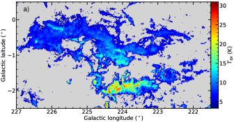
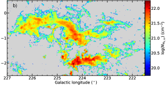
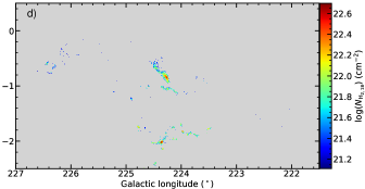
Figure 9: Maps of ($a$) excitation temperature distributions, H₂ column density distributions traced by ($b$) ¹²CO, ($c$) ¹³CO, and ($d$) C¹⁸O.

Similar to figure 5 of Barnes et al. (2018), in Figure 8(a), we have presented the results of our analysis of $X_{\mathrm{CO}}$ (i, j, v) for each channel (or voxel) and pixel (i.e., this calculation was conducted in 3D). Each black point represents a channel that showed both ¹³CO and ¹²CO detections. $N_{\rm H_{2}}$ and $I_{\mathrm{CO}}$ (i.e., $I_{\mathrm{CO}}$ = $T_{\mathrm{MB}}\times$0.168 km s^-1) were both calculated here per channel. Similar to figure 9 of Barnes et al. (2018), in Figure 8(b), have presented our results of our analysis of $N_{\rm H_{2}}$(i, j) for each pixel. Each quantity was integrated across all velocity channels with detectable ¹²CO emission, regardless of whether ¹³CO emission is detected.

The $X_{\mathrm{CO}}$ and $I_{\mathrm{CO}}$ relationships (shown in both panels of Figure 8) confirm that $X_{\mathrm{CO}}$ decreases as $I_{\mathrm{CO}}$ increases for faint $I_{\mathrm{CO}}$ (i.e. it has a negative slope), but $X_{\mathrm{CO}}$ increases as $I_{\mathrm{CO}}$ increases for brighter $I_{\mathrm{CO}}$ (i.e. a positive slope is seen). A caveat of this result is that the power-law fit to our data is unreliable due to the relatively small range that the $I_{\mathrm{CO}}$ data covers (i.e. $\sim$ an order of magnitude) and the large scatter of the data. Consequently, only the mean and median values of $X_{\mathrm{CO}}$ are indicated in each panel.

As discussed by Barnes et al. (2018), the relation in Figure 8(b) represents the practical conversion laws, since what is used is the total unmasked $I_{\mathrm{CO}}$ data across all velocity channels with detectable ¹²CO emission. Therefore, the derived $X_{\mathrm{CO}}$ factors derived from the voxels containing both ¹²CO and ¹³CO emission in Figure 8(a) represent upper limits. However, because a large velocity coverage integrated, any non-relevant components will enhance $I_{\mathrm{CO}}$ and lower $X_{\mathrm{CO}}$; thus, the derived $X_{\mathrm{CO}}$ conversion factors in the right panel represents lower limits.

As suggested by Sun et al. (2020), the practical X_CO conversion factor might fall in the range between the values in Figure 8(a–b). We have adopted a mean value of $X_{\mathrm{CO}}$ = 1.7 $\times$ 10²⁰ cm^-2 (K km s^-1)^-1 in this work. It should be noted that the derived value of $X_{\mathrm{CO}}$ largely depends on the uncertainties of the isotopic ratio of [¹²C/¹³C] and abundance ratio of [H₂]/[¹²CO]. Nevertheless, our value is still very similar to the value of 1.8 $\times$ 10²⁰ cm^-2 (K km s^-1)^-1 estimated by Dame et al. (2001) for the local gas.

Knowing the $N_{\rm H_{2}}$ value in each pixel, we then calculated the mass traced by each isotopologue by integrating the column density over the area of each mask region as:

$$M\ =\ 2\mu_{\mathrm{H}}m_{\mathrm{H}}a^{2}d^{2}\sum{N_{\mathrm{H_{2}}}}.$$ (6)

where $\mu_{\mathrm{H}}$ (=1.36, Hildebrand, 1983) is the mean atomic weight per proton in the interstellar medium (ISM) and $m_{\mathrm{H}}$ is the mass of proton. The molecular gas surface density, $\Sigma$, is simply the mass divided by the projected area, $\Sigma=M/A$.

The area ratios traced by ¹²CO, ¹³CO, and C¹⁸O were also calculated as $\mathbb{A}_{\rm 12}^{\rm 13}$=$A_{\rm{}^{13}CO}$/$A_{\rm{}^{12}CO}$, $\mathbb{A}_{\rm 12}^{\rm 18}$=$A_{\rm C^{18}O}$/$A_{\rm{}^{12}CO}$, where $A_{\rm{}^{12}CO}$, $A_{\mathrm{{}^{13}CO}}$, and $A_{\rm C^{18}O}$ are areas with detectable ¹²CO  (mask ‘B’), ¹³CO  (mask ‘G’), and C¹⁸O  (mask ‘R’) emission, respectively. Similarly, we also calculate the mass ratios, $\mathbb{M}_{\rm 12}^{\rm 13}$=$M_{\rm{}^{13}CO}$/$M_{\rm{}^{12}CO}$, $\mathbb{M}_{\rm 12}^{\rm 18}$=$M_{\rm C^{18}O}$/$M_{\rm{}^{12}CO}$, where $M_{\rm{}^{12}CO}$, $M_{\rm{}^{13}CO}$, and $M_{\rm C^{18}O}$ are the total masses contained in each area, respectively.

The derived properties of the molecular gas are all summarized in Tables 2–3. As expected, the excitation temperatures, column densities, and surface gas densities increase as we move from region ‘B’, i.e., the outskirts of MCs, to the denser regions ‘G’ and ‘R’. These statistical results are consistent with those revealed by Sun et al. (2020) in G130 region. In addition, the physical properties seem to vary considerably in different sub-regions. The H₂ column density, surface gas density, $\mathbb{A}_{\rm 12}^{\rm 18}$, and $\mathbb{M}_{\rm 12}^{\rm 18}$ in sub-region C are much smaller than those in the other two sub-regions. Such significant variations likely reflect the different levels of star-formation activities and/or the different evolutionary stages of the MCs.

Maps of excitation temperature and H₂ column density are also presented in Figure 9. It is noticeable that a large fraction of the area has the $T_{\rm ex}<$10 K. In addition, as the hottest region, sub-region A still has a mean value of $T_{\rm ex}$ below 10 K. This suggests that a considerable amount of the observed molecular gas is excited in regions with low excitation conditions, which was also suggested by many other studies (e.g., Goldsmith et al., 2008; Pineda et al., 2008).

3.3 Abundance Ratio

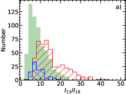
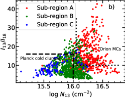
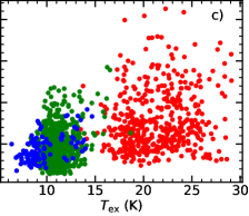
Figure 10: ($a$) Histograms of abundance ratios $X_{\rm{}^{13}CO}$/$X_{\rm C^{18}O}$ of all three sub-regions. ($b$) Relation between $X_{\rm{}^{13}CO}$/$X_{\rm C^{18}O}$ and $N_{\rm{}^{13}CO}$. The dashed and dotted lines indicate the approximate boundaries of type i and type ii MCs (Wang et al., 2019), respectively, into which the Planck cold clumps (Wu et al., 2012), and the Orion MCs fall into (Shimajiri et al., 2014). ($c$) Relation between $X_{\rm{}^{13}CO}$/$X_{\rm C^{18}O}$ and $T_{\rm ex}$. Note that only those pixels with both detectable ¹³CO and C¹⁸O emission (mask ‘R’ region) have been plotted.

Following the methodology adopted in previous studies (e.g.,  Shimajiri et al., 2014; Wang et al., 2019), in this section we systematically examined in this section the abundance ratio of [$\rm{}^{13}CO/C^{18}O$] assuming that the abundance ratio is proportional to the total integrated intensity ratio (with optical depth correction), $X_{\rm{}^{13}CO}$/$X_{\rm C^{18}O}\ \propto\ I_{13}/I_{18}$. The derived abundance ratios $X_{\rm{}^{13}CO}$/$X_{\rm C^{18}O}$ of all three sub-regions are plotted as histograms in Figure 10(a). The relationships between $X_{\rm{}^{13}CO}$/$X_{\rm C^{18}O}$ and $N_{\rm{}^{13}CO}$ are shown in Figure 10(b). In addition, Figure 10(c) presents the relationship between $X_{\rm{}^{13}CO}$/$X_{\rm C^{18}O}$ and $T_{\mathrm{ex}}$.

We find that the abundance ratios of $X_{\rm{}^{13}CO}$/$X_{\rm C^{18}O}$ have mean values of 15.4, 9.1, and 9.0, and median values of 13.6, 8.0, and 8.2, for sub-regions A, B, and C, respectively. These values are much larger than the solar system’s value (5.5), suggesting that UV photons from the nearby OB stars and/or Hii regions have a strong influence on the chemistry of clouds in the CMa OB1 complex. Since C¹⁸O is selectively dissociated by UV emission more effectively than ¹³CO, the abundance variations of these isotopologues across different environments have been interpreted as an indicator of the evolutionary stages of MCs (e.g., van Dishoeck & Black, 1988; Shimajiri et al., 2014). According to the relation $X_{\rm{}^{13}CO}$/$X_{\rm C^{18}O}$-$N_{\rm{}^{13}CO}$, Wang et al. (2019) defined two types of MCs. The boundaries of type i and type ii MCs are approximately indicated by the dashed and dotted lines in Figure 10(b). Type i MCs are characterized by a lower abundance ratio $X_{\rm{}^{13}CO}$/$X_{\rm C^{18}O}$, and lower ¹³CO column density with relatively lower excitation temperature than type ii MCs. Therefore, type i MCs are probably quiescent clouds or in the early stage of star formation. On the contrary, type ii MCs contain active star-forming MCs and are strongly influenced by newly formed stars. Clearly, we can classify sub-region C as a type i cloud, and sub-region A as a type ii cloud. Meanwhile, sub-region B appears to fall into a region between type i and type ii, where star-formation has occurred but the feedback from the young generation seems not significant. This view is supported by our results of the ongoing star-formation census in §5.

4 C¹⁸O clumps

4.1 Clump Identification

Since clumps/cores are the basic unit of star formation, they are helpful to understand the fragmentation and star formation of MCs (e.g.,  Bergin & Tafalla, 2007). The physical properties of the clumps/cores in the CMa OB1 complex were studied using the NANTEN CO and $Herschel/Hi-GAL$ data (e.g., Elia et al., 2013). Considering much denser gas it can probe than ¹²CO, C¹⁸O is more suitable for tracing compact molecular clumps/cores, which are more likely to form stars.

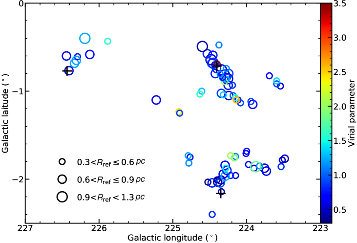
Figure 11: Distributions of C¹⁸O clumps. The circles and crosses represent the positions of the C¹⁸O clumps and the three known water masers, respectively.

We use the CUPID (part of the STARLINK project software) clump-finding algorithm GaussClumps (Stutzki, & Guesten, 1990) to identify compact clumps in the 3D FITS cube of C¹⁸O. We set the parameters MAXSKIP = 100, MINPIX = 8, and NPEAK = 5. Here, MAXSKIP determines the maximum amount of iterations that the Gaussian fits are performed. If the number of failed attempts to fit consecutive clumps reaches MAXSKIP, Gaussclumps stops searching for further clumps. A large value of MAXSKIP may allow the user to identify more clumps; however, it becomes more time consuming to do so. We tested three cases, MAXSKIP = 50, 100, and 400, which revealed that the number of clumps was the same for the latter two cases, and were both larger than MAXSKIP = 50. Therefore, we set MAXSKIP = 100 in this study. Next, MINPIX determines the minimum number of pixels each clump contains. Considering that a clump must contain at least one beam size (nearly four pixels) in the $l$-$b$ space, and at least two channels in velocity space, we finally use MINPIX = 8. NPEAK determines the minimum peak emission of each clump. We assumed a peak main beam temperature of each clump of $\geqslant$ 5$\sigma$. Thus, we take NPEAK = 5 as our final selection. Finally, 83 clumps in total were identified in the whole mapped area. The measured parameters of each clump including the position, central velocity ($V_{\rm LSR}$), angular size ($A$), velocity dispersion ($dv$), peak main beam temperatures of C¹⁸O ($T_{\mathrm{C}^{18}\mathrm{O}}$) and ¹²CO ($T_{{}^{12}\mathrm{CO}}$) are listed in Table A. The spatial distributions of these clumps are also shown in Figure 11, of which 32, 42, and nine C¹⁸O clumps are located at sub-regions A, B, and C, respectively.

4.2 Physical Properties of C¹⁸O Clumps

As stated in §3.2, here we also assume that $T_{\mathrm{ex}}$ is the same of all CO isotopologues. For simplicity, we also assume that $T_{\mathrm{ex}}$ and $\tau$ are uniform within each clump. Then following the Equations 1 and 3, we adopt the peak main beam temperatures of ¹²CO and C¹⁸O (columns 4 and 5 of Table A) to estimate $T_{\mathrm{ex}}$ and $\tau$ for each clump.

The effective radius obtained after beam deconvolution ($R_{\mathrm{eff}}$) is given by $R_{\mathrm{eff}}=d\times\sqrt{\frac{A}{\pi}-\frac{\theta_{\mathrm{MB}}^{2}}{4}}$, where $d$ is the distance (which was assumed to be 1.15 kpc), $\theta_{\mathrm{MB}}$ is the FWHM beam width, and $A$ is the angle area of each clump. Following MacLaren et al. (1988), virial mass $M_{\mathrm{vir}}$ can be estimated by $M_{\mathrm{vir}}=210R_{\mathrm{eff}}(\Delta v)^{2}$, where $\Delta v=\sqrt{8\ln 2}dv$. Virial parameter can be calculated by $\alpha_{\mathrm{vir}}$=$M_{\mathrm{vir}}$/$M_{\mathrm{LTE}}$. The derived physical properties are summarized in Table A.

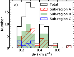
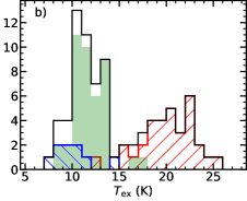
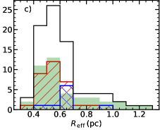
Figure 12: Histograms of physical properties of C¹⁸O clumps including ($a$) velocity dispersion, ($b$) excitation temperature, and ($c$) effective radius.

The distributions of $dv$, $T_{\rm ex}$, and radius of the 83 C¹⁸O clumps are also plotted as histograms in Figure 12. The velocity dispersions ($dv$) of the clumps are in the range of 0.17 to 0.72 km s^-1, with the mean value of 0.33 km s^-1. Only a few clumps are similar to clumps seen in infrared dark clouds (0.64–0.94 km s^-1 Zhang et al., 2011). While the majority clumps are similar to those clumps in low-mass protostars (0.13–0.89 km s^-1 Jørgensen et al., 2002). The clumps in sub-region A seem to have slightly larger values of $dv$ (mean value 0.35 km s^-1) than those clumps in sub-regions B (mean 0.33 km s^-1) and C (mean 0.26 km s^-1). The $T_{\rm ex}$ values of clumps in sub-region A are typically $\sim$ 20 K, which are also much higher than those in sub-regions B and C. Here, we should note that the conclusion for sub-region C is rather tentative, since the relatively small number of clumps in sub-region C (nine) likely restrict its statistical significance. The values of $R_{\mathrm{eff}}$ for all sub-regions is between 0.3 pc and 1.3 pc, with the mean value of 0.59 pc. We note that all of the detected C¹⁸O clumps are above our detection resolution limit of 0.14 pc, and match well with the definition of a clump, which have typical sizes of 0.3 pc $\leqslant$ $R_{\mathrm{eff}}~{}\leqslant$ 3 pc(Bergin & Tafalla, 2007). In contrast, the mean $R_{\mathrm{eff}}$ of “¹²CO clumps”, identified by Elia et al. (2013), is 4.79 pc, which actually matches typical cloud size.

To determine the dominant broadening mechanisms, we calculate both thermal velocity dispersion ($\sigma_{\mathrm{T}}$) and non-thermal velocity dispersion ($\sigma_{\mathrm{NT}}$) using the following equations (Myers, 1983; Li et al., 2015):

$$\sigma_{\mathrm{T}}\ =\ \frac{1}{1000}\sqrt{\frac{kT_{\mathrm{kin}}}{\mu m_{\mathrm{H}}}},$$ (7)

$$\sigma_{\mathrm{NT}}\ =\ \sqrt{dv^{2}-\left(\frac{1}{1000}\sqrt{\frac{kT_{\mathrm{kin}}}{m_{\mathrm{C^{18}O}}}}\right)^{2}},$$ (8)

where $k$ is the Boltzmann constant, $\mu=2.4$, $T_{\mathrm{kin}}$ is kinetic temperature, and $m_{\mathrm{C^{18}O}}$ is the mean molecular mass of C¹⁸O. We assumed $T_{\mathrm{ex}}$ as the lower limit of $T_{\mathrm{kin}}$ when estimating $\sigma_{\rm Non-thermal}$ and $\sigma_{\rm Thermal}$, which thus also both represent lower limits.

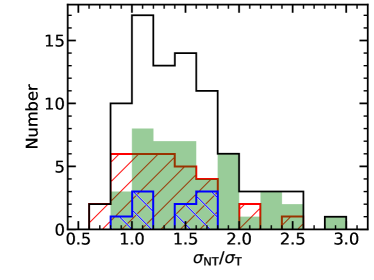
Figure 13: Histograms of the ratio between non-thermal (blue) and thermal (red) velocity dispersions of the 83 C¹⁸O clumps. The color codes are same as in Figure 12.

Figure 13 presents the ratios between $\sigma_{\rm NT}$ and $\sigma_{\rm T}$ for each sub-region. Our statistical results reveal that 68 (82%) clumps have $\sigma_{\mathrm{NT}}$ values larger than $\sigma_{\mathrm{T}}$. Additionally, the ratios between $\sigma_{\mathrm{NT}}$ and $\sigma_{\mathrm{T}}$ of the C¹⁸O clumps are in the range of 0.64 to 2.84, with an average value of 1.44, and a median value of 1.37, which implies that non-thermal broadening mechanism may play a dominant role in the CMa OB1 complex. In addition, we find that the clumps in sub-region B have the highest values of $\sigma_{\mathrm{NT}}$ to $\sigma_{\mathrm{T}}$ ratios (with an average value of 1.57, and median value of 1.46). Meanwhile, the $\sigma_{\mathrm{NT}}$ to $\sigma_{\mathrm{T}}$ ratios of the clumps in sub-region C (with an average value of 1.33, and median value of 1.47) have slightly larger values than those of sub-region A (with an average value of 1.30, and median value of 1.25). However, as mentioned above, due to the limited number of clumps in sub-region C, the conclusion for sub-region C should be viewed with caution.

The virial parameter of each clump is illustrated in Figure 11. We find about 78 (94%) clumps have $\alpha_{\rm vir}<$2, which are thought to be gravitationally bound. This implies that these clumps may eventually collapse into stars. In comparison, only 7% of the “¹²CO clumps” observed by Elia et al. (2013) were found to be gravitationally bound in the CMa OB1 complex. As mentioned above, the “¹²CO clumps” with an average radii of several parsecs actually represent typical MCs. Therefore, the discrepancy between the C¹⁸O clumps and “¹²CO clumps” may lend support to the view that molecular clumps (i.e., the site in which star formation to take place) within MCs should be gravitationally bound; however, it is not necessary that the MCs as a whole be bound (e.g.,  Clark & Bonnell, 2005; Ballesteros-Paredes et al., 2011). Moreover, our results show the advantage of C¹⁸O in tracing high density components.

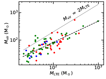
Figure 14: Virial mass $M_{\mathrm{vir}}$ as a function of LTE mass $M_{\mathrm{LTE}}$ for C¹⁸O clump. The color codes are same as in Figure 12.

The relationship between $M_{\mathrm{LTE}}$ and $M_{\mathrm{vir}}$ is shown in Figure 14. The dashed line indicates the best-fitting power-law to all the 83 C¹⁸O clumps, computed using a least-squares bisector. The power index is 0.77$\pm$0.06, and the Pearson correlation coefficient of relation is 0.8. We find that the virial parameters of C¹⁸O clumps tend to decrease with the increase of LTE masses. This indicates that C¹⁸O clumps with larger LTE masses are more likely to be gravitationally bound.

The core/clump mass function (CMF) is an empirical function which describes the relative frequency of cores/clumps with different masses. CMF resembles the stellar initial mass function (IMF) which describes the initial distributions of masses of a stellar population. The CMF is defined as:

$$N(\log M)\propto M^{\alpha},$$ (9)

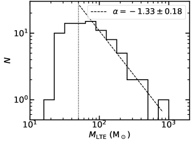
Figure 15: Clump mass distribution in the CMa OB1 complex. The dotted line masks the minimum meaningful mass with a value of 50 M_☉.

where $N$ is the number of clumps per bin, and $M$ is the LTE mass here. For our case, we use the Markov Chain Monte Carlo (MCMC) algorithm to estimate the power-law index (Koen & Kondlo, 2009; Yan et al., 2020). We set the minimum meaningful mass as 50 M_⊙, and use 54 clumps to calculate the power-law index of the CMF. We calculate two MCMC sampling chains with a total of 2000 sample numbers. Consequently, the power-law index was found to be $\alpha=-1.33\pm$0.18 for the high-mass portion of the mass distribution of the C¹⁸O clumps (see Figure 15). Unlike the result of $\alpha=-0.7\pm$ 0.3 based on “¹²CO clumps” found by Elia et al. (2013), the result derived from our C¹⁸O clumps is more in agreement with that of the Hi-GAL pre-stellar sources in the CMa OB1 complex ($\alpha=-1.0\pm$0.2, Elia et al., 2013). In addition, the constrained CMF of the C¹⁸O clumps in the CMa OB1 complex is similar to that of nearby star-forming regions, e.g., $\alpha=-1.3\pm$0.1 in Orion A (Ikeda et al., 2007), $\alpha=-1.3\pm$0.2 in Perseus, Serpens, and Ophiuchus (Enoch et al., 2008).

Furthermore, we see that all those observed CMFs (from this study and literature) resemble several typical IMF, e.g., $\alpha=-1.35$ (Salpeter, 1955), $\alpha=-1.3\pm$0.7 for single stars (Kroupa, 2001), and $\alpha=-1.35\pm$0.3 for multiple systems (Chabrier, 2005). Such similarity between the CMF and IMF may imply that the CMF can impact the origin of the IMF to some extent via turbulent fragmentation, which is consistent with the prediction of turbulent fragmentation theories (which have been used to explain the CMF and cloud structure at various scales, Offner et al., 2014).

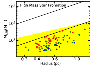
Figure 16: Mass–size relationship of C¹⁸O clumps in the CMa OB1 complex. The upper and lower black lines represent the empirical surface densities required for high-mass star formation with values of 1 g cm^-2 (Krumholz & McKee, 2008) and 0.05 g cm^-2 (Urquhart et al., 2013), respectively. The yellow shaded region represents the region where low-mass star formation is more likely to take place (Kauffmann & Pillai, 2010). The color codes are same as in Figure 12.

To examine how many clumps have the potential to form high-mass stars, we have presented the mass–size relation of the C¹⁸O clumps in Figure 16. The upper and lower black solid lines indicate constant surface densities of 1 g cm^-2 (Krumholz & McKee, 2008) and 0.05 g cm^-2 (Urquhart et al., 2013), respectively. If these two lines provide the reliable empirical upper and lower bounds for the clump surface densities required for massive star formation, then none of the C¹⁸O clump has enough surface densities to form high-mass stars. Besides, when the empirical relationship suggested by Kauffmann & Pillai (2010) is considered, all of C¹⁸O clumps still lie in the region where low-mass star formation is more likely to take place. These results would suggest that none of the C¹⁸O clump has the potential to form high-mass stars in CMa OB1 complex.

5 Outflow Candidates

5.1 Identification of outflow candidates

Outflow is a universal phenomenon in star-forming regions, arising from deeply embedded protostellar objects to optically visible young stars (Reipurth & Bally, 2001). CO spectral lines can reveal outflow activities in star-forming regions (e.g.,  Shu et al., 1987), and compared to optical outflows, CO outflows occur during the younger stages (Ginsburg et al., 2011). Large-scale outflows surveys can provide a large systematic sample for investigating the impact of outflow activities on their surrounding environments (e.g.,  Arce et al., 2010). Therefore, studying the large-scale properties of MCs and their associated star-forming activities are necessary. However, to date there is no CO outflow survey in the CMa OB1 complex.

In this section, we identify ¹²CO molecular outflows by using a set of semi-automated IDL algorithm based on 3D $l-b-v$ data of ¹²CO and ¹³CO (Li et al., 2018, 2019). This algorithm suite allows the user to determine the central velocity and minimum velocity extents of each pixel by fitting optically-thin ¹³CO lines. Then, the CUPID clump-finding algorithm is used to automatically identify any extreme points (i.e., points that have maximum velocity extents compared with surrounding) in ¹²CO data (see details in Li et al., 2018, 2019). Using such line and artificial diagnoses method, we search for and identify outflow candidates. Then, we inspected the maps (e.g., intensity map, P–V diagram, and/or channel map) of each candidate by eye to exclude those with ambiguous outflow characteristics (e.g., outflow extent velocities $<$ 1 km s^-1) or those seriously contaminated by other components. In this step, about 2/3 raw outflow samples that automatically from the procedure are excluded. Eventually, only 56 blue-lobe and 52 red-lobe candidates are included in this study. If the separation between a blue-lobe and a red-lobe was smaller than 1.5 pc, then they were paired to constitute a bipolar outflow candidate. Finally, we identify 85 outflow candidates in the CMa OB1 complex, including 23 bipolar outflow candidates, 33 blue and 29 red monopolar ones (see Appendix B). All of these are new detections.

A search using the SIMBAD database revealed that only those three outflow candidates associated with water masers (bipolar outflow candidates 43 and 47, and red monopolar candidates 83) were single-pointing observed via SiO line by Harju et al. (1998) (in their table B1, indices of 19–21). Their observations resulted in SiO detections of each of these three candidates, which had SiO line widths up to 23.8 km s^-1. Moreover, only outflow candidate 47 was previously observed via NH₃ line (Tatematsu et al., 2017).

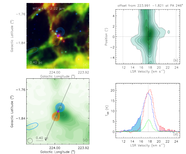
Figure 17: An example outflow candidate (No. 25). ($a$) Integral intensity maps of the red and blue lobes superposed on the WISE image (blue, green, and red for 4.6, 12, and 22 $\mu$m, respectively). ($b$) P–V diagram along position angle of the outflow marked at the top the panel. ($c$) Integral intensity maps of the red and blue lobes superposed on the ¹³CO intensity map. The arrow indicates the position angle of the outflow. ($d$) ¹²CO spectra at the peak emission of the blue and red lobes are coded in blue and red, respectively, while the green one is the averaged ¹³CO spectrum over 3$\,\times\,$3 pixels centered at the position of the outflow. The line wing velocity range of each lobe is specified with shading.

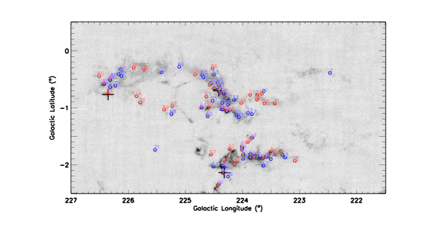
Figure 18: Locations of outflow candidates. The grey-scale map presents the integrated intensity of ¹³CO line, integrated over (0, 30) km s^-1. The blue and red circles represent the positions of the blue and red lobes, respectively. The green bars connect the blue and red lobes of the bipolar outflow candidates. The blue/red and purple number present the index of blue/red monopolar and bipolar outflow candidates, respectively. The black crosses represent of positions of the three known water masers (Brand et al., 1994).

The measured parameters for each outflow candidate are summarized in Table B. Figure 17 presents the details of outflow candidate with the index of 25 as an example, and the spatial distributions of all detected ¹²CO outflow candidates are shown in Figure 18. Apparently, the outflow candidates are mainly distributed along filaments in the CMa OB1 complex. Additionally, we find that the outflows are not uniformly distributed in different sub-regions, and they are clearly concentrated in sub-regions A and B. Using the equations listed in Appendix B of Li et al. (2018), the outflow candidates’ physical parameters were also calculated and tabulated in Table C. It is also worth noting that the calculated masses, momenta, and energies are lower limits, due to underestimated low-velocity outflows, as discussed in detail in section 4.2 of Li et al. (2018).

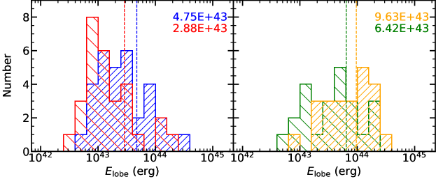
Figure 19: Histograms of the kinetic energy of the outflow lobes. The hatched regions in left panel show the distributions of the red-lobes (in red, sub-group 1) and blue-lobes (in blue, sub-group 3) of the monopolar outflow candidates, while the hatched regions in right panel show the red-lobes (in green, sub-group 2) and blue-lobes (in yellow, sub-group 4) of the bipolar outflow candidates. The mean values of each sub-group are also indicated in each panel.

The 56+52 detected outflow lobes were split into four sub-groups: (1) 29 red-lobes from monopolar outflows, (2) 23 red-lobes from bipolar outflows, (3) 33 blue-lobes from monopolar outflows, and (4) 23 blue-lobes from bipolar outflows. A comparison of the velocities, masses, kinetic energies, dynamical timescales and luminosities for the four sub-groups is shown in Table 4. We find that lobes from the bipolar outflow candidates (sub-groups 2 and 4) generally have larger velocities, masses, kinetic energies, and luminosities than those lobes of the monopolar outflow candidates (sub-groups 1 and 3). Overall, the velocities of two lobes of bipolar outflows are symmetrical. However, no significant difference between the lobes from bipolar and monopolar outflows was found in properties of dynamic timescale. The kinetic-energy distributions, which exhibit significant differences between the 4 sub-groups, are also presented in Figure 19, which are plotted in different colors. The mean values of each sub-group are also indicated in each panel. These findings are similar to the statistical results in Gemini OB1 (Li et al., 2018) and W3/4/5 complex (Li et al., 2019), implying that the components of bipolar outflows are more massive, and thus more easily detectable.

5.2 Star formation activity in the CMa OB1 complex

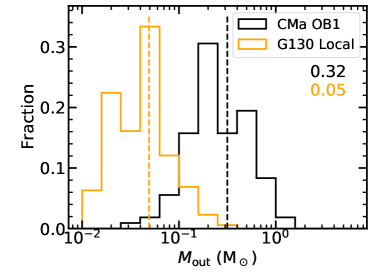
Figure 20: Histograms of the mass of the outflow candidates in the CMa OB1 complex, and in G130 local MCs (Li et al., 2019)

Histograms of the outflow masses for the CMa OB1 complex are presented in Figure 20. For comparison, we have also overlaid a histogram of the local MCs in the G130 region (as mentioned in §3.2), which have a mean distance of $\sim$600 pc. (Li et al., 2019; Sun et al., 2020). The outflow masses range from 0.01 to 1.19 M_⊙, with an average value of 0.32 M_⊙ for the entire CMa OB1 complex, which obviously have higher masses than G130 local MCs. Since the two studies using data with uniform quality and the same identification method, the outflow census may indicate that the CMa OB1 complex represents an active star-forming region in the Local arm. Considering that the classification of an outflow is performed based on its mass (see Yang et al., 2018), we suggest that the detected outflows in this study are likely to be dominated by intermediate- or low-mass outflows.

To quantify the level of star-formation activity in different sub-regions, and for the whole region, we further carried out a statistical analysis. Herein, we have defined the number of outflows per unit area ($\eta_{\rm out}$) and per unit mass ($\zeta_{\rm out}$), as $\eta_{\rm out}=N_{\rm out}$/$A_{\rm{}^{12}CO}$, and $\zeta_{\rm out}=N_{\rm out}$/$M_{\rm{}^{12}CO}$, respectively, where $N_{\rm out}$ is the number of outflow candidates, and $A_{\rm{}^{12}CO}$ and $M_{\rm{}^{12}CO}$ are the same parameters as defined in §3.2. Similarly, we define the outflow mass fraction, $\mathbb{M}_{\rm 12}^{\rm out}$ ($\mathbb{M}_{\rm 12}^{\rm out}$=$M_{\rm out}/M_{\rm{}^{12}CO}$), as the ratio of the mass of outflow and molecular gas derived from ¹²CO. All these parameters ($\eta_{\rm out}$, $\zeta_{\rm out}$, and $M_{\rm out}^{\rm 12}$), may offer valuable insights to the level of star-formation activity within MCs. The derived parameters for the CMa OB1 complex and its sub-regions, and the G130 Local MCs from literature, are listed in Table 5.

The results show that the value of$\eta_{\rm out}$ corresponding to the whole CMa OB1 complex is almost the same as that of the relatively more nearby G130 local MCs (0.037 pc^-2; Li et al., 2019; Sun et al., 2020). The values of $\eta_{\rm out}$ of sub-regions A and B are similar and both larger than that of sub-region C. Meanwhile, sub-region B possesses the largest number of outflows per unit mass. As expected, sub-region C has the lowest value of $M_{\rm out}^{\rm 12}$, while the remaining two sub-regions have similar values. All these strongly suggest that star-formation in sub-regions A and B are obviously more active relative to that in sub-region C from the view of outflow activities. Since star formation is thought to be closely related to the amount of dense gas present, we suggest that significant variation of the mass ratio $M_{\mathrm{C^{18}O}}$/$M_{\mathrm{{}^{12}CO}}$ (refer to Table 3) may largely contribute to the outflow discrepancy across different sub-regions (refer to Table 5).

For our mapped region, sub-regions A and C are outside the spitzer/Herschel fields. And in sub-region B, a total of 293 YSOs were identified by Sewiło et al. (2019), which resulted in the number YSOs per unit area ($\eta_{Y}$) of 0.31 pc^-2. We further defined a conversion factor $C^{\rm Y}_{\rm O}$ here (defined as the ratio $\eta_{\rm YSO}$/$\eta_{\rm out}$), which is estimated to be $\sim$7.8 for sub-region B. Since YSOs are always associated with outflows in nearby star-forming regions (Curtis et al., 2010), this conversion factor might reflect the relative completeness of the YSOs and/or outflows. The disagreement between YSOs and outflows may indicate that we are likely to identify clustered outflows as single or extended lobes, and/or fail to see the faint outflows. Toward the more nearby MCs, e.g., the Perseus molecular cloud complex, the $C^{Y}_{O}$ with value of $\sim$ 5.3$=$1.05/0.20 (distance 250 pc; Arce et al., 2010), and the Taurus molecular cloud with value of $\sim$ 6.5$=$1.36/0.21 (distance 140 pc; Li et al., 2015), are both very similar to that of the CMa OB1 complex. This may suggest that MWISP data with improved sensitivity are therefore able to detect outflows at a distance of 1150 pc comparable to nearby Perseus and Taurus.

6 Correlation between the compact C¹⁸O clumps and the outflow candidates

If a C¹⁸O clump overlapped with a monopolar outflow candidate (both spatially and in terms of velocity), we assume that this C¹⁸O clump are correlated with the monopolar outflow candidate. And for bipolar outflow candidate, due to the central position of bipolar outflow candidate may easily confirm the parent MC, only the central position of bipolar outflow candidate located in C¹⁸O clump, we assume that this C¹⁸O clump is correlated with the bipolar outflow candidate. Consequently, we find 47 C¹⁸O clumps (57%) correlate with the outflow candidates. The correlation between the C¹⁸O clumps and the outflow candidates are also presented in column 15 of Table A.

Table 6 presents the physical parameters of the dense C¹⁸O clumps with and without associated outflow candidates. We find that the C¹⁸O clumps with associated outflow candidates (i.e., the first sub-group) showed higher masses than the C¹⁸O clumps without associated outflow candidates (i.e., the second sub-group). There are no significant differences in the other properties (i.e., $dv$, $T_{\mathrm{ex}}$, $\sigma_{\rm NT}$/$\sigma_{\rm T}$, $R_{\mathrm{eff}}$, $\alpha_{\mathrm{vir}}$) between the two categories.

There are 37 outflow candidates (44%) correlated with the C¹⁸O clumps, including 16 bipolar outflow candidates (70%), 11 blue (33%) and 10 red (34%) monopolar ones. Similarly, the statistical outflow properties of the outflow candidates with and without associated C¹⁸O clumps are presented in Table 7. The lobe candidates with associated C¹⁸O clumps have slightly higher velocities, masses, kinetic energies, and luminosities than the lobes without associated C¹⁸O clumps. However, the differences are still within their respective standard deviation (i.e., 1.31 km s^-1, 0.23 M_☉, 6.66E+43 erg and 1.73E+32 erg s^-1, respectively).

7 Summary

Using ¹²CO/¹³CO/C¹⁸O data from the ongoing MWISP project, we have reported a study of the CMa OB1 complex (with sky coverage of 16.5 deg² in total), including a detail analysis of large-scale distributions and properties of molecular gas, and diagnosis of the C¹⁸O clumps and CO molecular outflows. In this study, the CMa OB1 complex was roughly divided into three sub-regions according to the morphology of ¹³CO emission. The main results and conclusions of this study are summarized as follows:

(1) The total H₂ masses of the mapped area traced by the ¹²CO, ¹³CO, and C¹⁸O emission were estimated to be 8.5 $\times\ 10^{4}$, 6.5 $\times\ 10^{4}$, and 6.6 $\times\ 10^{3}~{}\mathrm{M}_{\sun}$, respectively. A large fraction of the observed molecular gas is emitted from regions with low excitation conditions. A comparative study of the physical properties of the CMa OB1 complex reveals evidence for significant varying excitation temperature, H₂ column density, surface gas density, $A_{\rm 18}^{\rm 12}$, and $M_{\rm 18}^{\rm 12}$ in different sub-regions. The mean abundance ratio of $X_{\rm{}^{13}CO}$/$X_{\rm C^{18}O}$ was estimated to be 14.9 for the entire mapped region, which is much larger than that of the solar system value (5.5). Additionally, this ratio seemed to vary in different sub-regions, indicating different evolutionary stages of MCs in the CMa OB1 complex.

(2) A total of 83 C¹⁸O clumps are identified using GaussClumps algorithm. A non-thermal broadening mechanism was found to play an important role in the detected C¹⁸O clumps. We found about 94% of the clumps are gravitationally bound and may collapse to form stars. The size–mass relation of the clumps indicates that the C¹⁸O clumps in the CMa OB1 complex are unlikely to form high-mass stars. The power index of the C¹⁸O clump mass function, $N(\log M)\propto M^{\alpha}$, is found to be –1.33$\pm$0.18, which is similar to that of the Hi-GAL pre-stellar sources in the CMa OB1 complex ($\alpha$=–1.0$\pm$0.2, Elia et al., 2013), and also resembles the initial mass distribution function in the Milk Way.

(3) A total of 85 outflow candidates were identified using a semi-automatic IDL algorithm, of which all were new detections, and 23 were bipolar outflow candidates. The total outflow mass of the mapped area was estimated to be 34.1 M_☉. Our outflow census indicated that the CMa OB1 complex represents an active star-forming region in the Local arm. Our comparative study reveals that the level of star formation activity in the CMa OB1 complex seems to be closely related to the amount of relatively denser gas traced by C¹⁸O.

Table 1: Observed properties of each region

Observed properties	Sub-region A				Sub-region B					Sub-region C
	12CO	13CO	C18O		12CO	13CO	C18O		12CO	13CO	C18O
$V_{\rm LSR}$ (km s-1)	17.2	17.2	16.9		15.3	15.5	14.6		16.2	16.3	16.6
$\Delta V$ (km s-1)	3.1	2.6	2.5		3.8	3.1	2.1		3.6	2.8	3.2
$A$ ($10^{2}$ arcmin2)	54.7	22.5	1.2		84.5	31.1	1.5		52.0	23.5	0.3
$I$ (K km s-1 arcmin-2)	8.0E4	9.7E3	1.2E2		7.9E4	9.6E3	2.1E2		4.7E4	5.3E3	0.2E2

Note. — Rows 1–2: Central velocity, and corresponding FWHM line width of the averaged ¹²CO/¹³CO/C¹⁸O spectra in each sub-region. Note that the averaged spectra of C¹⁸O in sub-regions A and C, are not Gaussian-like, thus the FWHM line widths marked with “$\dagger$” may be overestimated. Rows 3–4: Total area and total integrated intensity traced by ¹²CO/¹³CO/C¹⁸O in each sub-region.

Table 2: Statistics of excitation temperature, log[$N_{\mathrm{H_{2}}}$], mass, and surface density.

Sub-region	Mask		$T_{\mathrm{ex}}$				log[$N_{\mathrm{H_{2}}}$]		$M$	$\Sigma$
	Region	min	max	mean		min	max	mean
		(K)				(cm-2)			($\times$103 M⊙)	(M⊙ pc-2)
A	B	3.5	30.9	9.9		20.1	22.3	21.2	32.9	53.9
	G	4.1	30.9	14.7		20.2	22.7	21.3	28.3	113.2
	R	9.6	29.1	21.1		21.2	22.7	21.8	2.7	192.9
B	B	3.4	18.8	7.4		19.7	22.1	21.0	32.5	34.6
	G	4.1	18.8	9.6		20.2	22.4	21.1	23.7	67.7
	R	8.1	18.7	11.1		21.1	22.5	21.7	3.6	200.2
C	B	3.3	21.7	7.1		20.1	22.0	21.1	19.4	32.9
	G	4.1	21.7	8.6		20.2	22.2	21.1	13.0	48.1
	R	6.4	14.7	9.7		21.2	22.0	21.4	0.3	110.8

Table 3: Area and mass ratios.

Sub-region	$\mathbb{A}_{12}^{\rm 13}$	$\mathbb{M}_{12}^{\rm 13}$	$\mathbb{A}_{12}^{\rm 18}$	$\mathbb{M}_{\rm 12}^{\rm 18}$
	(%)	(%)	(%)	(%)
A	41.2	86.0	2.2	8.2
B	36.8	72.9	1.8	11.1
C	45.3	67.0	0.5	1.5

Note. — Refer to §3.2 for the definations of the area and mass ratios.

Table 4: Statistics of outflow properties for the four sub-groups

Sub-group	Number		$\langle\Delta v_{\mathrm{lobe}}\rangle$			$M_{\mathrm{lobe}}$			$E_{\mathrm{lobe}}$			$t_{\mathrm{lobe}}$			$L_{\mathrm{lobe}}$
			mean	median		mean	median		mean	median		mean	median		mean	median
			(km s-1)			(M⊙)			(erg)			(yr)			(erg s-1)
1	29		3.24	2.93		0.20	0.16		2.88E+43	1.15E+43		2.20E+05	1.92E+05		7.04E+30	2.22E+30
2	23		4.26	4.17		0.29	0.22		6.42E+43	4.36E+43		1.68E+05	1.25E+05		1.77E+31	9.27E+30
3	33		-3.39	-3.26		0.31	0.26		4.75E+43	2.27E+43		2.72E+05	2.26E+05		9.06E+30	4.00E+30
4	23		-4.13	-4.08		0.50	0.43		9.63E+43	8.75E+43		2.23E+05	1.78E+05		1.66E+31	1.08E+31

Note. — Sub-groups 1–4 respectively represent: the (1) 29 red-lobes from monopolar outflows, (2) 23 red-lobes from bipolar outflows, (3) 33 blue-lobes from monopolar outflows, and (4) 23 blue-lobes from bipolar outflows.

.

Table 5: Statistics of outflow candidates

Region	Monopolar	Bipolar	$N_{\rm out}$	$M_{\rm out}$	$\eta_{\rm out}$	$\zeta_{\rm out}$	$\mathbb{M}_{\rm 12}^{\rm out}$
					$\times 10^{\rm-2}$	$\times$10-4	$\times$10-4
	(B/R)			(M☉)	(pc-2)	(M${}_{\sun}^{-1}$)
sub-region A	9/9	11	29	13.2	4.7	8.8	4.01
sub-region B	16/12	9	37	15.1	3.9	11.4	4.65
sub-region C	8/8	3	19	5.8	3.2	9.7	2.99
whole region	33/29	23	85	34.1	3.7	10.0	4.02
G130 Local	55/95	12	162	17.8	3.7	17.1	1.80

Note. — Refer to §5.2 for the definitions of each column. Please refer to Li et al. (2019) and Sun et al. (2020) for the statistical results for the local MCs in the G130 region ($l$=[129$\fdg$75, 140$\fdg$25] and $b$=[$-$5$\fdg$25, +5$\fdg$25]).

Table 6: Statistical parameters of the C¹⁸O clumps with and without associated outflow candidates.

clump	number		$dv$			$T_{\mathrm{ex}}$			$\sigma_{\mathrm{NT}}$/$\sigma_{\mathrm{T}}$			$R_{\mathrm{ref}}$			$M_{\mathrm{LTE}}$			$\alpha_{\mathrm{vir}}$
			mean	median		mean	median		mean	median		mean	median		mean	median		mean	median
			(km s-1)			(K)						(pc)			(M⊙)
Correlated	47		0.34	0.32		15.26	13.38		1.46	1.35		0.64	0.60		126	86		0.96	0.80
Uncorrelated	36		0.31	0.28		14.45	13.15		1.32	1.17		0.54	0.50		70	49		1.08	0.92
Total	83		0.33	0.31		14.90	13.38		1.40	1.30		0.59	0.53		102	68		1.01	0.85

Table 7: Statistical parameters of the lobe candidates with and without associated C¹⁸O clumps.

lobe	number		$\langle\Delta v_{\mathrm{lobe}}\rangle$			$M_{\mathrm{lobe}}$			$P_{\mathrm{lobe}}$			$E_{\mathrm{lobe}}$			$t_{\mathrm{lobe}}$			$L_{\mathrm{lobe}}$
			mean	median		mean	median		mean	median		mean	median		mean	median		mean	median
(B/R)			(km s-1)			(M⊙)			(M⊙ km s-1)			(erg)			(yr)			(erg s-1)
Correlated B	27		-3.87	-3.86		0.44	0.37		1.82	1.71		7.96E+43	6.43E+43		2.28E+05	2.02E+05		1.41E+31	8.23E+30
Uncorrelated B	29		-3.52	-3.46		0.34	0.24		1.31	0.78		5.63E+43	2.68E+43		2.74E+05	2.47E+05		1.04E+31	3.76E+30
Total B	56		-3.69	-3.69		0.39	0.32		1.56	1.00		6.75E+43	3.68E+43		2.51E+05	2.12E+05		1.22E+31	6.45E+30
Correlated R	26		4.44	4.22		0.32	0.25		1.50	1.01		7.60E+43	4.42E+43		1.69E+05	1.25E+05		2.11E+31	1.08E+31
Uncorrelated R	26		2.93	2.78		0.15	0.14		0.42	0.39		1.29E+43	1.05E+43		2.26E+05	1.97E+05		2.42E+30	1.55E+30
Total R	52		3.69	3.32		0.24	0.18		0.96	0.58		4.45E+43	2.04E+43		1.97E+05	1.75E+05		1.17E+31	2.63E+30

Appendix A The physical properties of C¹⁸O clumps.

Table A: The physical properties of C¹⁸O clumps

Clump	$V_{\mathrm{LSR}}$	$dv$	$T_{\mathrm{C}^{18}\mathrm{O}}$	$T_{{}^{12}\mathrm{CO}}$	$A$	$T_{\mathrm{ex}}$	$\tau$	$\sigma_{\mathrm{T}}$	$\sigma_{\mathrm{NT}}$	$R_{\mathrm{eff}}$	$M_{\mathrm{LTE}}$	$M_{\mathrm{vir}}$	$\alpha_{\mathrm{vir}}$	Outflow Index
Name	(km s-1)	(km s-1)	(K)	(K)	(arcmin2)	(K)		(km s-1)	(km s-1)	(pc)	(M⊙)	(M⊙)
(1)	(2)	(3)	(4)	(5)	(6)	(7)	(8)	(9)	(10)	(11)	(12)	(13)	(14)	(15)
G223.483-01.767	18.78	0.33	2.00	14.73	10.11	18.17	0.15	0.25	0.32	0.58	131	72	0.55
G223.517-01.783	18.66	0.28	2.19	14.93	7.31	18.38	0.16	0.25	0.27	0.49	90	45	0.50	8,16
G223.533-01.858	18.78	0.27	1.38	18.18	6.20	21.64	0.08	0.27	0.25	0.44	42	37	0.88	7
G223.542-00.942	16.44	0.17	1.81	5.62	7.31	8.92	0.39	0.18	0.16	0.49	28	16	0.58
G223.592-00.883	15.94	0.25	1.34	6.81	5.94	10.15	0.22	0.19	0.25	0.43	22	32	1.45
G223.592-00.917	16.27	0.20	1.34	6.83	9.13	10.16	0.22	0.19	0.19	0.55	27	25	0.91	10
G223.692-00.825	13.28	0.20	1.35	7.20	8.50	10.54	0.21	0.19	0.19	0.53	33	24	0.75
G223.733-01.908	17.27	0.34	1.87	16.82	11.87	20.28	0.12	0.27	0.33	0.63	140	84	0.60	16
G223.758-01.875	17.27	0.33	1.73	16.42	12.99	19.87	0.11	0.26	0.33	0.66	149	86	0.58	16
G223.825-01.850	17.45	0.41	1.58	13.67	9.13	17.11	0.12	0.24	0.40	0.55	90	107	1.19	19,20
G223.875-01.858	18.11	0.72	1.27	18.72	23.77	22.19	0.07	0.28	0.71	0.91	298	540	1.82	19,20
G223.900-01.875	17.91	0.29	1.75	18.82	8.81	22.29	0.10	0.28	0.28	0.54	87	51	0.59
G223.917-01.150	15.61	0.26	1.48	9.45	12.99	12.84	0.17	0.21	0.25	0.66	75	52	0.70
G223.942-01.117	15.11	0.24	1.29	10.16	5.94	13.55	0.13	0.22	0.23	0.43	29	28	0.95	22
G223.975-01.833	17.94	0.43	2.07	19.82	7.60	23.30	0.11	0.28	0.42	0.50	164	109	0.66	25
G224.000-01.683	17.27	0.23	1.45	19.22	8.19	22.69	0.08	0.28	0.22	0.52	51	33	0.66	27
G224.008-01.708	16.79	0.33	1.98	14.96	7.60	18.41	0.14	0.25	0.32	0.50	87	61	0.70	26,27
G224.083-01.133	16.09	0.29	1.63	10.52	6.74	13.92	0.17	0.22	0.29	0.47	49	47	0.96	29,30
G224.117-01.100	15.31	0.35	2.13	9.51	8.50	12.90	0.25	0.21	0.34	0.53	99	74	0.75	30
G224.142-01.100	16.78	0.46	1.34	6.01	7.31	9.32	0.25	0.18	0.46	0.49	45	120	2.67
G224.150-01.075	14.78	0.44	1.55	10.07	7.60	13.46	0.17	0.22	0.43	0.50	68	111	1.63
G224.150-01.742	18.30	0.39	1.80	13.30	5.44	16.74	0.14	0.24	0.38	0.41	60	71	1.18
G224.150-01.958	18.46	0.25	1.90	18.97	5.69	22.45	0.11	0.28	0.24	0.42	53	32	0.60	31,32
G224.167-01.758	19.61	0.55	1.50	16.54	8.50	20.00	0.10	0.26	0.54	0.53	93	183	1.97
G224.183-01.050	14.60	0.35	1.70	10.37	7.60	13.77	0.18	0.22	0.35	0.50	68	73	1.07
G224.192-00.933	13.11	0.21	1.41	8.12	7.60	11.48	0.19	0.20	0.20	0.50	27	25	0.90
G224.217-01.733	20.62	0.35	1.35	9.05	5.94	12.43	0.16	0.21	0.35	0.43	29	63	2.13	35
G224.217-01.958	16.94	0.28	1.49	14.13	5.19	17.57	0.11	0.25	0.27	0.40	42	37	0.89
G224.242-00.800	14.45	0.26	1.44	7.60	10.80	10.95	0.21	0.19	0.26	0.60	53	48	0.91
G224.242-01.050	14.79	0.41	2.77	9.98	21.26	13.38	0.32	0.22	0.41	0.86	317	169	0.53	34,39
G224.250-00.933	13.61	0.31	1.47	8.56	15.80	11.94	0.19	0.20	0.30	0.73	107	82	0.77	37
G224.258-00.842	15.60	0.27	1.47	7.90	3.64	11.26	0.20	0.20	0.26	0.33	27	27	1.00
G224.258-00.858	14.09	0.58	3.61	8.59	43.89	11.96	0.54	0.20	0.58	1.24	979	487	0.50	38
G224.267-01.900	17.28	0.33	1.27	15.84	12.24	19.29	0.08	0.26	0.32	0.64	103	80	0.78
G224.275-00.742	14.12	0.25	1.39	7.57	8.19	10.92	0.20	0.19	0.24	0.52	32	38	1.18
G224.275-00.867	15.12	0.33	1.42	8.52	7.60	11.89	0.18	0.20	0.33	0.50	48	65	1.34	38
G224.283-01.875	18.94	0.56	1.30	18.27	8.19	21.73	0.07	0.27	0.55	0.52	124	190	1.52
G224.292-01.842	19.11	0.27	1.27	18.17	11.50	21.64	0.07	0.27	0.26	0.62	71	52	0.74
G224.292-01.967	16.95	0.30	1.29	16.05	11.15	19.50	0.08	0.26	0.29	0.61	51	65	1.28	41
G224.300-00.817	14.26	0.48	2.41	8.13	41.12	11.50	0.35	0.20	0.48	1.20	460	324	0.70
G224.300-00.892	13.95	0.49	1.43	8.33	3.44	11.70	0.19	0.20	0.49	0.31	40	90	2.24	38
G224.317-01.042	14.95	0.37	1.41	9.87	8.81	13.26	0.15	0.21	0.37	0.54	64	87	1.37	45
G224.317-01.942	16.95	0.21	1.43	12.35	12.24	15.78	0.12	0.23	0.20	0.64	51	34	0.67	41
G224.325-00.842	15.28	0.18	1.39	7.79	7.31	11.14	0.20	0.20	0.17	0.49	26	17	0.67
G224.325-00.850	13.60	0.33	1.39	8.95	5.19	12.32	0.17	0.21	0.32	0.40	37	50	1.34
G224.342-00.758	14.62	0.30	1.78	7.47	32.16	10.82	0.27	0.19	0.29	1.06	208	110	0.53	42
G224.342-01.025	15.94	0.44	2.20	10.06	18.43	13.45	0.25	0.22	0.43	0.80	197	177	0.90	45
G224.342-02.142	16.62	0.32	2.20	19.73	8.50	23.21	0.12	0.28	0.31	0.53	123	63	0.51	43
G224.350-02.008	16.91	0.46	2.85	17.10	15.38	20.56	0.18	0.27	0.45	0.72	370	176	0.48	44
G224.358-00.808	14.62	0.28	1.32	8.44	6.47	11.81	0.17	0.20	0.27	0.45	35	41	1.19
G224.358-02.042	16.95	0.47	1.72	20.99	10.45	24.47	0.09	0.29	0.46	0.59	158	148	0.93	44
G224.375-00.475	14.12	0.24	1.39	4.94	7.02	8.22	0.33	0.17	0.24	0.48	28	32	1.15
G224.392-02.033	16.64	0.22	1.79	16.37	20.29	19.83	0.12	0.26	0.21	0.84	138	49	0.36
G224.400-00.692	13.44	0.49	1.27	9.06	8.19	12.44	0.15	0.21	0.49	0.52	40	144	3.61	47,51
G224.400-02.008	17.27	0.20	1.56	19.23	5.19	22.71	0.08	0.28	0.18	0.40	42	18	0.44
G224.408-00.742	15.94	0.42	2.04	8.21	16.65	11.57	0.28	0.20	0.42	0.75	186	158	0.85	47
G224.425-00.800	15.28	0.26	1.44	10.23	10.80	13.63	0.15	0.22	0.25	0.60	57	46	0.81
G224.433-00.700	15.77	0.23	1.73	9.59	8.50	12.98	0.20	0.21	0.22	0.53	49	32	0.65	47,51
G224.450-00.683	15.10	0.27	1.45	7.30	24.82	10.65	0.22	0.19	0.27	0.93	98	81	0.83	51,52,57
G224.458-00.592	15.77	0.26	1.50	7.64	12.61	10.99	0.22	0.20	0.26	0.65	68	53	0.79	50
G224.467-02.042	17.61	0.47	1.82	17.16	10.80	20.62	0.11	0.27	0.46	0.60	190	152	0.80	54
G224.467-02.400	9.94	0.33	1.50	21.91	8.19	25.40	0.07	0.30	0.32	0.52	76	65	0.86	49
G224.475-00.683	16.24	0.45	2.09	7.47	15.80	10.82	0.33	0.19	0.44	0.73	152	170	1.11	51,52,57
G224.483-00.642	15.60	0.31	1.66	7.32	31.56	10.66	0.26	0.19	0.31	1.05	228	120	0.53	51,52
G224.525-02.033	17.40	0.24	2.73	15.38	9.13	18.83	0.19	0.26	0.22	0.55	105	35	0.34	54
G224.533-00.575	15.44	0.27	1.47	7.06	18.89	10.40	0.23	0.19	0.27	0.81	83	69	0.83	58
G224.600-00.492	15.44	0.18	1.31	6.07	23.26	9.38	0.24	0.18	0.17	0.90	76	32	0.42
G224.608-01.000	16.93	0.49	1.57	14.10	5.94	17.54	0.12	0.25	0.48	0.43	86	119	1.39	59
G224.633-01.033	16.94	0.48	1.44	13.38	5.19	16.81	0.11	0.24	0.48	0.40	63	109	1.72
G224.767-01.750	15.60	0.41	2.40	17.18	7.02	20.65	0.15	0.27	0.40	0.48	142	93	0.65
G224.783-01.817	15.79	0.30	1.44	12.24	5.69	15.66	0.13	0.23	0.29	0.42	36	43	1.21
G224.792-01.733	15.27	0.44	1.64	19.49	4.95	22.97	0.09	0.28	0.43	0.39	69	90	1.30
G224.908-01.250	12.61	0.24	1.30	9.28	7.89	12.66	0.15	0.21	0.23	0.51	36	33	0.92
G224.917-01.233	13.27	0.42	1.40	10.13	7.60	13.52	0.15	0.22	0.41	0.50	40	100	2.53
G225.225-01.100	13.94	0.18	1.30	7.82	13.37	11.18	0.18	0.20	0.17	0.67	42	26	0.61	68
G225.883-00.433	15.78	0.28	1.28	5.64	6.74	8.94	0.26	0.18	0.27	0.47	25	42	1.65
G226.125-00.583	18.60	0.17	1.25	3.99	11.87	7.23	0.37	0.16	0.17	0.63	30	22	0.72
G226.192-00.400	15.61	0.28	1.28	5.15	25.35	8.43	0.28	0.17	0.28	0.94	72	89	1.23	78
G226.292-00.608	16.45	0.21	1.36	5.70	8.19	9.00	0.27	0.18	0.20	0.52	32	26	0.80	81
G226.308-00.650	17.61	0.32	1.26	7.40	14.16	10.75	0.19	0.19	0.31	0.69	65	81	1.24	81
G226.333-00.683	17.93	0.31	1.45	5.73	11.15	9.04	0.29	0.18	0.31	0.61	56	69	1.24	81
G226.408-00.767	15.45	0.20	1.57	6.88	11.87	10.21	0.26	0.19	0.19	0.63	53	30	0.56
G226.442-00.600	15.44	0.34	1.98	11.27	11.15	14.69	0.19	0.23	0.34	0.61	121	85	0.70	84

Note–

• Column (1): Name of each clump, as defined by its central Galactic Coordinates.

• Columns (2)–(3): Central velocity and velocity dispersion of each clump.

• Column (4): Angular area of each clump, estimated by GaussClumps.

• Column (5): Peak main beam temperature of the C¹⁸O emission peak fitted by GaussClumps.

• Column (6): Main beam temperature of ¹²CO peak within the same area of clumps in ¹²CO data.

• Columns (7)-(14): Excitation temperature, optical depth, thermal velocity dispersion, non-thermal velocity dispersion, effective radius, LTE mass, virial mass, and virial parameter of each clump (see details in §4.2)

• Column (15): Index of associated Outflow candidate (Table B, C col. 1).

Appendix B The Outflow Candidates

Table B: The outflow candidates.

Index	$l$	$b$	bw0	bw1	rw0	rw1	tag
	(deg)	(deg)	(km s-1)	(km s-1)	(km s-1)	(km s-1)
(1)	(2)	(3)	(4)	(5)	(6)	(7)	(8)
1	222.468	-0.391	14.1	15.2	$\cdots$	$\cdots$	B
2	223.084	-1.934	$\cdots$	$\cdots$	18.6	20.2	R
3	223.254	-1.874	15.1	16.6	$\cdots$	$\cdots$	B
4	223.313	-1.794	13.8	16.3	20.1	21.7	D
5	223.434	-1.823	$\cdots$	$\cdots$	20.6	24.0	R
6	223.436	-0.924	$\cdots$	$\cdots$	18.4	21.1	R
7	223.503	-1.904	12.8	14.6	$\cdots$	$\cdots$	B
8	223.513	-1.774	$\cdots$	$\cdots$	20.3	21.6	R
9	223.590	-1.863	13.4	15.5	$\cdots$	$\cdots$	B
10	223.616	-0.928	$\cdots$	$\cdots$	17.6	19.2	R
11	223.629	-2.016	11.6	15.5	$\cdots$	$\cdots$	B
12	223.643	-0.733	10.0	11.8	15.3	17.1	D
13	223.646	-1.885	12.6	14.9	19.8	22.4	D
14	223.742	-0.773	$\cdots$	$\cdots$	15.9	17.1	R
15	223.745	-0.859	$\cdots$	$\cdots$	14.7	17.4	R
16	223.749	-1.870	13.0	15.1	19.4	22.0	D
17	223.835	-1.113	12.1	14.4	$\cdots$	$\cdots$	B
18	223.840	-1.527	14.6	16.8	21.1	22.3	D
19	223.856	-1.829	12.3	14.8	20.3	21.7	D
20	223.859	-1.884	12.1	15.7	$\cdots$	$\cdots$	B
21	223.866	-0.773	$\cdots$	$\cdots$	14.2	17.3	R
22	223.903	-1.090	12.0	13.7	$\cdots$	$\cdots$	B
23	223.909	-1.600	$\cdots$	$\cdots$	20.4	21.7	R
24	223.991	-1.898	14.6	15.8	$\cdots$	$\cdots$	B
25	223.991	-1.821	11.8	15.9	20.1	23.9	D
26	224.008	-1.732	12.1	15.7	18.9	21.3	D
27	224.010	-1.681	11.7	15.2	19.4	23.5	D
28	224.022	-0.916	$\cdots$	$\cdots$	14.8	17.4	R
29	224.063	-1.165	10.8	13.6	$\cdots$	$\cdots$	B
30	224.108	-1.129	10.8	13.7	$\cdots$	$\cdots$	B
31	224.109	-1.954	$\cdots$	$\cdots$	20.6	23.3	R
32	224.146	-1.998	$\cdots$	$\cdots$	20.6	24.7	R
33	224.149	-0.863	8.0	10.4	$\cdots$	$\cdots$	B
34	224.222	-1.041	$\cdots$	$\cdots$	18.4	23.7	R
35	224.227	-1.725	$\cdots$	$\cdots$	22.1	24.8	R
36	224.256	-2.209	14.8	16.4	$\cdots$	$\cdots$	B
37	224.259	-0.951	8.0	12.1	$\cdots$	$\cdots$	B
38	224.272	-0.839	6.9	11.0	19.3	24.1	D
39	224.276	-1.066	7.3	11.0	19.4	25.1	D
40	224.317	-2.050	12.1	13.9	$\cdots$	$\cdots$	B
41	224.317	-1.953	$\cdots$	$\cdots$	20.2	22.7	R
42	224.330	-0.747	8.5	12.0	18.6	24.4	D
43	224.340	-2.143	10.5	15.4	19.4	24.9	D
44	224.350	-2.017	9.7	13.6	20.1	24.7	D
45	224.354	-1.030	8.6	13.9	18.4	21.7	D
46	224.356	-0.915	6.7	12.5	$\cdots$	$\cdots$	B
47	224.407	-0.721	7.1	11.8	19.4	22.4	D
48	224.415	-0.616	10.1	13.4	$\cdots$	$\cdots$	B
49	224.422	-2.351	5.8	7.6	11.4	14	D
50	224.435	-0.559	10.3	12.6	$\cdots$	$\cdots$	B
51	224.469	-0.671	$\cdots$	$\cdots$	19.5	22.4	R
52	224.492	-0.662	8.3	13.4	19.4	23.1	D
53	224.500	-0.417	10.1	13.3	$\cdots$	$\cdots$	B
54	224.508	-2.034	14.1	15.8	$\cdots$	$\cdots$	B
55	224.526	-0.879	12.3	13.5	$\cdots$	$\cdots$	B
56	224.526	-0.308	$\cdots$	$\cdots$	17.3	19.1	R
57	224.551	-1.820	$\cdots$	$\cdots$	20.9	23.4	R
58	224.561	-0.581	10.3	13.1	17.6	22.0	D
59	224.594	-0.984	$\cdots$	$\cdots$	20.3	26.7	R
60	224.607	-1.151	12.9	15.9	$\cdots$	$\cdots$	B
61	224.633	-0.805	$\cdots$	$\cdots$	17.8	20.9	R
62	224.685	-0.466	9.8	13.6	$\cdots$	$\cdots$	B
63	224.706	-0.426	9.3	13.4	$\cdots$	$\cdots$	B
64	224.717	-0.997	12.3	16.8	19.4	21.8	D
65	224.833	-0.419	$\cdots$	$\cdots$	19.4	20.7	R
66	225.109	-0.283	12.1	14.9	$\cdots$	$\cdots$	B
67	225.229	-0.974	$\cdots$	$\cdots$	15.8	17.2	R
68	225.246	-1.110	10.0	12.6	$\cdots$	$\cdots$	B
69	225.373	-1.034	$\cdots$	$\cdots$	16.2	17.7	R
70	225.417	-0.377	12.5	14.3	$\cdots$	$\cdots$	B
71	225.533	-1.739	13.4	14.6	$\cdots$	$\cdots$	B
72	225.726	-0.332	$\cdots$	$\cdots$	19.0	21.2	R
73	225.792	-0.910	$\cdots$	$\cdots$	16.3	17.7	R
74	225.859	-0.799	$\cdots$	$\cdots$	16.1	18.9	R
75	225.907	-0.293	$\cdots$	$\cdots$	18.1	19.7	R
76	226.120	-0.343	11.1	13.4	19.3	20.6	D
77	226.122	-0.443	9.6	13.1	$\cdots$	$\cdots$	B
78	226.170	-0.408	11.0	13.8	$\cdots$	$\cdots$	B
79	226.225	-0.615	12.6	15.8	$\cdots$	$\cdots$	B
80	226.283	-0.466	6.0	13.1	$\cdots$	$\cdots$	B
81	226.319	-0.637	13.8	15.3	$\cdots$	$\cdots$	B
82	226.323	-0.507	9.3	12.1	18.3	22.2	D
83	226.356	-0.758	$\cdots$	$\cdots$	18.7	22.7	R
84	226.427	-0.584	8.5	12.8	19.6	23.8	D
85	226.511	-0.447	$\cdots$	$\cdots$	18.6	21.6	R

Note–

• Column (1): Index of outflow candidate.

• Column (2)-(3): Central Galactic coordinates of outflow candidate.

• Columns (4)-(5): Velocity range of the blue line wing.

• Columns (6)-(7): Velocity range of the red line wing.

• Column (8): Type of outflow candidate, where “B”, “R”, and “D” denote blue-, red-monopolar, and bipolar outflow candidates, respectively.

Appendix C Parameters of Outflow Candidates

Table C: Physical properties of the Outflow Candidates

Index	Lobe	$l$	$b$	$v_{\mathrm{peak}}$	$\psi$	$A_{\mathrm{lobe}}$	$\langle\Delta v_{\mathrm{lobe}}\rangle$	$l_{\mathrm{lobe}}$	$M_{\mathrm{lobe}}$	$P_{\mathrm{lobe}}$	$E_{\mathrm{lobe}}$	$t_{\mathrm{lobe}}$	$L_{\mathrm{lobe}}$
		(deg)	(deg)	(km s-1)		(arcmin2)	(km s-1)	(pc)	(M⊙)	(M⊙ km s-1)	(erg)	(yr)	(erg s-1)
(1)	(2)	(3)	(4)	(5)	(6)	(7)	(8)	(9)	(10)	(11)	(12)	(13)	(14)
1	B	222.468	-0.391	16.16	0.75	1.47	-1.62	0.72	3.66E-02	5.94E-02	9.54E+41	3.41E+05	8.87E+28
2	R	223.084	-1.934	17.60	0.75	2.17	1.64	0.87	3.45E-01	5.65E-01	9.18E+42	3.28E+05	8.87E+29
3	B	223.254	-1.874	17.82	0.60	7.33	-2.12	1.60	4.43E-01	9.40E-01	1.98E+43	5.76E+05	1.09E+30
4	B	223.302	-1.826	17.80	0.50	4.39	-3.00	1.24	2.06E-01	6.20E-01	1.84E+43	3.03E+05	1.93E+30
	R	223.324	-1.763	18.12	0.50	2.11	2.62	0.86	1.29E-01	3.37E-01	8.76E+42	2.35E+05	1.18E+30
5	R	223.434	-1.823	18.10	0.50	1.28	3.86	0.67	1.55E-01	5.97E-01	2.29E+43	1.11E+05	6.53E+30
6	R	223.436	-0.924	15.39	0.50	2.64	4.09	0.96	1.77E-01	7.24E-01	2.94E+43	1.65E+05	5.65E+30
7	B	223.503	-1.904	16.69	0.50	5.25	-3.17	1.36	2.67E-01	8.47E-01	2.66E+43	3.41E+05	2.48E+30
8	R	223.513	-1.774	18.61	0.50	3.08	2.21	1.04	1.59E-01	3.51E-01	7.67E+42	3.41E+05	7.14E+29
9	B	223.590	-1.863	17.27	0.60	4.28	-3.03	1.22	4.30E-01	1.30E+00	3.91E+43	3.10E+05	4.00E+30
10	R	223.616	-0.928	16.24	0.75	2.17	2.00	0.87	1.35E-01	2.70E-01	5.37E+42	2.88E+05	5.92E+29
11	B	223.629	-2.016	17.77	0.60	4.67	-4.61	1.28	4.75E-01	2.19E+00	9.98E+43	2.03E+05	1.56E+31
12	B	223.626	-0.710	13.81	0.50	4.64	-3.09	1.28	1.83E-01	5.66E-01	1.74E+43	3.27E+05	1.68E+30
	R	223.660	-0.756	13.82	0.75	1.64	2.20	0.76	8.61E-02	1.89E-01	4.13E+42	2.26E+05	5.80E+29
13	B	223.658	-1.893	17.60	0.50	5.69	-4.08	1.41	5.30E-01	2.16E+00	8.75E+43	2.76E+05	1.00E+31
	R	223.634	-1.877	17.47	0.50	2.22	3.37	0.88	1.23E-01	4.16E-01	1.39E+43	1.75E+05	2.51E+30
14	R	223.742	-0.773	13.60	0.50	2.14	2.78	0.87	5.50E-02	1.53E-01	4.22E+42	2.42E+05	5.53E+29
15	R	223.745	-0.859	12.97	0.85	1.81	2.81	0.80	1.92E-01	5.40E-01	1.50E+43	1.76E+05	2.71E+30
16	B	223.737	-1.856	17.08	0.50	9.11	-3.24	1.79	1.07E+00	3.46E+00	1.11E+44	4.28E+05	8.23E+30
	R	223.761	-1.885	16.99	0.60	2.61	3.45	0.96	1.82E-01	6.28E-01	2.15E+43	1.87E+05	3.64E+30
17	B	223.835	-1.113	16.01	0.90	1.44	-2.99	0.71	1.02E-01	3.04E-01	9.03E+42	1.78E+05	1.61E+30
18	B	223.827	-1.521	18.28	0.50	4.47	-2.80	1.25	4.23E-01	1.18E+00	3.29E+43	3.32E+05	3.14E+30
	R	223.853	-1.533	19.22	0.50	1.89	2.36	0.81	1.80E-01	4.23E-01	9.89E+42	2.59E+05	1.21E+30
19	B	223.857	-1.814	17.25	0.50	3.28	-3.95	1.07	2.95E-01	1.17E+00	4.56E+43	2.12E+05	6.83E+30
	R	223.855	-1.845	18.30	0.50	5.06	2.56	1.33	3.96E-01	1.01E+00	2.57E+43	3.83E+05	2.12E+30
20	B	223.859	-1.884	17.34	0.75	4.17	-3.80	1.21	4.49E-01	1.71E+00	6.43E+43	2.25E+05	9.04E+30
21	R	223.866	-0.773	12.29	0.80	2.08	3.15	0.85	1.35E-01	4.26E-01	1.33E+43	1.67E+05	2.53E+30
22	B	223.903	-1.090	14.72	0.60	3.36	-2.04	1.09	2.55E-01	5.20E-01	1.05E+43	3.90E+05	8.55E+29
23	R	223.909	-1.600	19.37	0.50	3.14	1.55	1.05	1.18E-01	1.82E-01	2.80E+42	4.41E+05	2.01E+29
24	B	223.991	-1.898	16.90	0.50	4.83	-1.82	1.30	3.90E-01	7.09E-01	1.28E+43	5.54E+05	7.32E+29
25	B	223.986	-1.810	17.58	0.50	1.86	-4.14	0.81	4.88E-01	2.02E+00	8.29E+43	1.37E+05	1.92E+31
	R	223.996	-1.833	17.56	0.50	1.75	4.06	0.78	2.67E-01	1.08E+00	4.36E+43	1.21E+05	1.14E+31
26	B	224.007	-1.720	17.03	0.55	1.78	-3.49	0.79	3.02E-01	1.05E+00	3.64E+43	1.57E+05	7.37E+30
	R	224.010	-1.743	17.27	0.75	2.00	2.59	0.84	1.86E-01	4.81E-01	1.24E+43	2.03E+05	1.93E+30
27	B	224.008	-1.687	16.94	0.50	1.58	-3.84	0.75	1.65E-01	6.33E-01	2.41E+43	1.39E+05	5.48E+30
	R	224.013	-1.676	16.77	0.50	1.83	4.27	0.80	1.89E-01	8.06E-01	3.41E+43	1.17E+05	9.27E+30
28	R	224.022	-0.916	12.58	0.95	1.39	3.26	0.70	1.06E-01	3.46E-01	1.12E+43	1.42E+05	2.50E+30
29	B	224.063	-1.165	14.78	0.75	5.42	-2.86	1.38	8.02E-01	2.29E+00	6.49E+43	3.39E+05	6.07E+30
30	B	224.108	-1.129	15.35	0.70	1.75	-3.39	0.78	1.99E-01	6.73E-01	2.26E+43	1.68E+05	4.25E+30
31	R	224.109	-1.954	18.08	0.50	2.14	3.60	0.87	1.50E-01	5.41E-01	1.93E+43	1.62E+05	3.77E+30
32	R	224.146	-1.998	18.38	0.50	3.53	3.86	1.11	2.25E-01	8.71E-01	3.34E+43	1.72E+05	6.14E+30
33	B	224.149	-0.863	13.45	0.60	3.06	-4.49	1.04	1.72E-01	7.72E-01	3.43E+43	1.86E+05	5.86E+30
34	R	224.222	-1.041	14.70	0.70	1.50	5.82	0.73	4.16E-01	2.42E+00	1.40E+44	7.89E+04	5.61E+31
35	R	224.227	-1.725	20.81	0.50	5.39	2.37	1.37	4.25E-01	1.01E+00	2.36E+43	3.37E+05	2.22E+30
36	B	224.256	-2.209	17.18	0.75	3.86	-1.74	1.16	3.57E-01	6.20E-01	1.07E+43	4.79E+05	7.06E+29
37	B	224.259	-0.951	13.50	0.90	1.39	-3.86	0.70	2.16E-01	8.33E-01	3.19E+43	1.24E+05	8.15E+30
38	B	224.260	-0.838	14.32	0.50	6.72	-5.78	1.54	9.02E-01	5.21E+00	2.98E+44	2.02E+05	4.67E+31
	R	224.284	-0.840	13.97	0.50	3.39	7.25	1.09	3.94E-01	2.86E+00	2.06E+44	1.05E+05	6.19E+31
39	B	224.277	-1.072	14.57	0.50	3.83	-5.79	1.16	4.79E-01	2.77E+00	1.59E+44	1.56E+05	3.24E+31
	R	224.275	-1.059	14.80	0.50	2.14	6.88	0.87	4.52E-01	3.11E+00	2.12E+44	8.22E+04	8.17E+31
40	B	224.317	-2.050	16.47	0.75	1.47	-3.65	0.72	1.09E-01	3.98E-01	1.44E+43	1.61E+05	2.85E+30
41	R	224.317	-1.953	17.07	0.50	3.19	4.13	1.06	2.37E-01	9.78E-01	4.01E+43	1.84E+05	6.91E+30
42	B	224.328	-0.752	14.78	0.75	1.56	-4.88	0.74	2.28E-01	1.11E+00	5.37E+43	1.15E+05	1.48E+31
	R	224.332	-0.742	14.81	0.50	4.22	6.11	1.22	6.79E-01	4.15E+00	2.51E+44	1.24E+05	6.40E+31
43	B	224.341	-2.138	16.62	0.55	1.94	-4.16	0.83	6.23E-01	2.59E+00	1.07E+44	1.32E+05	2.57E+31
	R	224.338	-2.148	16.68	0.50	2.25	4.92	0.89	5.57E-01	2.74E+00	1.34E+44	1.06E+05	4.01E+31
44	B	224.354	-2.016	16.79	0.50	2.25	-5.53	0.89	3.68E-01	2.04E+00	1.12E+44	1.23E+05	2.89E+31
	R	224.347	-2.018	16.79	0.55	2.39	5.15	0.92	3.16E-01	1.63E+00	8.32E+43	1.13E+05	2.33E+31
45	B	224.365	-1.031	15.57	0.65	3.31	-4.85	1.08	7.15E-01	3.47E+00	1.67E+44	1.51E+05	3.50E+31
	R	224.342	-1.030	15.55	0.50	4.50	4.17	1.26	2.75E-01	1.15E+00	4.74E+43	2.00E+05	7.51E+30
46	B	224.356	-0.915	16.11	0.80	3.61	-7.09	1.13	6.32E-01	4.48E+00	3.14E+44	1.17E+05	8.51E+31
47	B	224.415	-0.710	14.78	0.50	5.56	-5.80	1.40	6.93E-01	4.02E+00	2.31E+44	1.78E+05	4.12E+31
	R	224.399	-0.732	15.26	0.60	2.39	5.34	0.92	1.60E-01	8.56E-01	4.53E+43	1.25E+05	1.15E+31
48	B	224.415	-0.616	15.15	0.85	2.22	-3.73	0.88	4.13E-01	1.54E+00	5.68E+43	1.71E+05	1.05E+31
49	B	224.409	-2.338	8.30	0.50	2.75	-1.78	0.98	2.40E-01	4.28E-01	7.56E+42	3.84E+05	6.24E+29
	R	224.435	-2.363	9.56	0.50	4.11	2.88	1.20	9.03E-01	2.60E+00	7.44E+43	2.64E+05	8.92E+30
50	B	224.435	-0.559	15.13	0.65	6.22	-3.91	1.48	5.32E-01	2.08E+00	8.05E+43	2.99E+05	8.53E+30
51	R	224.454	-0.680	15.02	0.50	7.53	5.64	1.62	5.29E-01	2.99E+00	1.67E+44	2.15E+05	2.46E+31
52	B	224.483	-0.663	15.17	0.55	2.11	-4.83	0.86	4.28E-01	2.06E+00	9.87E+43	1.23E+05	2.55E+31
	R	224.500	-0.661	15.35	0.50	1.64	5.53	0.76	1.48E-01	8.17E-01	4.48E+43	9.57E+04	1.48E+31
53	B	224.500	-0.417	16.42	0.90	1.47	-5.04	0.72	1.61E-01	8.10E-01	4.05E+43	1.11E+05	1.15E+31
54	B	224.508	-2.034	17.23	0.85	1.50	-2.45	0.73	2.21E-01	5.42E-01	1.32E+43	2.26E+05	1.84E+30
55	B	224.526	-0.879	15.22	0.65	2.94	-2.44	1.02	1.09E-01	2.67E-01	6.46E+42	3.40E+05	6.02E+29
56	R	224.526	-0.308	15.05	0.80	1.81	2.97	0.80	8.23E-02	2.44E-01	7.18E+42	1.92E+05	1.18E+30
57	R	224.551	-1.820	18.97	0.50	1.67	2.93	0.76	1.35E-01	3.96E-01	1.15E+43	1.69E+05	2.16E+30
58	B	224.544	-0.563	15.28	0.50	8.47	-3.86	1.72	6.96E-01	2.68E+00	1.03E+44	3.39E+05	9.59E+30
	R	224.579	-0.599	15.28	0.85	1.75	4.08	0.78	2.23E-01	9.09E-01	3.68E+43	1.14E+05	1.02E+31
59	R	224.594	-0.984	17.12	0.50	1.89	5.74	0.81	4.20E-01	2.41E+00	1.37E+44	8.31E+04	5.23E+31
60	B	224.607	-1.151	17.36	0.65	2.14	-3.26	0.87	1.31E-01	4.27E-01	1.38E+43	1.90E+05	2.30E+30
61	R	224.633	-0.805	16.27	0.50	6.19	2.77	1.47	3.56E-01	9.86E-01	2.71E+43	3.12E+05	2.75E+30
62	B	224.685	-0.466	15.61	0.65	1.69	-4.29	0.77	2.04E-01	8.74E-01	3.71E+43	1.30E+05	9.07E+30
63	B	224.706	-0.426	15.77	0.50	7.64	-4.83	1.64	8.35E-01	4.04E+00	1.93E+44	2.47E+05	2.48E+31
64	B	224.719	-0.993	17.82	0.55	2.50	-3.72	0.94	4.13E-01	1.54E+00	5.66E+43	1.66E+05	1.08E+31
	R	224.716	-1.000	17.82	0.50	3.78	2.54	1.15	2.21E-01	5.61E-01	1.41E+43	2.83E+05	1.58E+30
65	R	224.833	-0.419	15.81	0.55	2.92	4.11	1.01	7.10E-02	2.92E-01	1.19E+43	2.02E+05	1.86E+30
66	B	225.109	-0.283	15.96	0.55	5.92	-2.74	1.44	2.43E-01	6.68E-01	1.82E+43	3.65E+05	1.58E+30
67	R	225.229	-0.974	14.52	0.55	6.42	1.84	1.50	2.19E-01	4.03E-01	7.34E+42	5.48E+05	4.25E+29
68	B	225.246	-1.110	13.67	0.50	6.44	-2.63	1.50	3.11E-01	8.17E-01	2.13E+43	4.00E+05	1.69E+30
69	R	225.373	-1.034	14.14	0.75	1.39	2.66	0.70	5.74E-02	1.53E-01	4.02E+42	1.92E+05	6.64E+29
70	B	225.417	-0.377	15.94	0.50	2.94	-2.72	1.02	8.73E-02	2.37E-01	6.40E+42	2.89E+05	7.02E+29
71	B	225.533	-1.739	15.28	0.50	3.42	-1.40	1.09	2.38E-01	3.32E-01	4.59E+42	5.71E+05	2.55E+29
72	R	225.726	-0.332	16.79	0.60	1.64	3.09	0.76	6.97E-02	2.15E-01	6.60E+42	1.68E+05	1.24E+30
73	R	225.792	-0.910	14.30	0.90	2.56	2.56	0.95	1.46E-01	3.74E-01	9.51E+42	2.72E+05	1.11E+30
74	R	225.859	-0.799	14.50	0.90	1.39	2.72	0.70	1.49E-01	4.06E-01	1.09E+43	1.55E+05	2.23E+30
75	R	225.907	-0.293	16.09	0.80	1.69	2.65	0.77	1.42E-01	3.77E-01	9.92E+42	2.09E+05	1.51E+30
76	B	226.128	-0.323	15.48	0.65	2.92	-3.46	1.01	2.26E-01	7.82E-01	2.68E+43	2.26E+05	3.76E+30
	R	226.112	-0.362	15.59	0.95	1.69	4.23	0.77	6.83E-02	2.89E-01	1.21E+43	1.51E+05	2.55E+30
77	B	226.122	-0.443	15.53	0.50	4.69	-4.53	1.28	5.11E-01	2.32E+00	1.04E+44	2.11E+05	1.56E+31
78	B	226.170	-0.408	15.70	0.85	2.78	-3.58	0.99	2.65E-01	9.48E-01	3.36E+43	2.05E+05	5.19E+30
79	B	226.225	-0.615	17.34	0.85	1.67	-3.46	0.76	1.91E-01	6.62E-01	2.27E+43	1.58E+05	4.57E+30
80	B	226.283	-0.466	15.07	0.65	1.61	-6.23	0.75	3.37E-01	2.10E+00	1.30E+44	8.10E+04	5.08E+31
81	B	226.319	-0.637	16.70	0.75	1.92	-2.30	0.82	1.62E-01	3.72E-01	8.46E+42	2.77E+05	9.69E+29
82	B	226.320	-0.516	14.59	0.50	9.44	-4.17	1.82	1.19E+00	4.97E+00	2.05E+44	3.36E+05	1.94E+31
	R	226.325	-0.498	14.78	0.75	1.75	5.08	0.78	1.95E-01	9.92E-01	4.99E+43	1.03E+05	1.53E+31
83	R	226.356	-0.758	15.61	0.90	1.39	4.69	0.70	1.79E-01	8.38E-01	3.90E+43	9.63E+04	1.28E+31
84	B	226.420	-0.579	14.93	0.50	3.81	-4.71	1.16	6.10E-01	2.87E+00	1.34E+44	1.76E+05	2.41E+31
	R	226.434	-0.590	15.05	0.50	2.22	6.23	0.88	2.39E-01	1.49E+00	9.19E+43	9.88E+04	2.95E+31
85	R	226.511	-0.447	17.38	0.50	3.19	2.42	1.06	1.59E-01	3.84E-01	9.21E+42	2.45E+05	1.19E+30

Note–

• Column (1): Index of outflow candidate.

• Column (2): Type of lobe candidate, where “B”, and “R” denote blue and red lobe candidate, respectively.

• Columns (3)–(4): Central Galactic coordinates of lobe candidate.

• Column (5): Velocity of ¹²CO peak emission.

• Column (6): Lowest contour boundary of each lobe, ranges from 50% to 95% of the peak intensity. For the isolated lobes, we use $\psi=0.5$. If a lobe candidate suffered from confusion due to adjacent components, then a higher value of $\psi$ was tested to ensure that the lobe could be distinguished from the cloud.

• Column (7): Angular area of each lobe, defined by the lowest contour level of each lobe.

• Columns (8)-(14): Velocity, length, mass, momentum, kinetic energy, dynamical timescale, and luminosity of each outflow candidate. As suggested by many outflow studies (e.g., Snell et al., 1984; Li et al., 2018, 2019), we assume a constant $T_{\mathrm{ex}}$ of 30 K for all detected outflow candidates.

References

- Arce et al. (2010) Arce, H. G., Borkin, M. A., Goodman, A. A., et al. 2010, ApJ, 715, 1170
- Ballesteros-Paredes et al. (2011) Ballesteros-Paredes, J., Hartmann, L. W., Vázquez-Semadeni, E., et al. 2011, MNRAS, 411, 65
- Barnes et al. (2015) Barnes, P. J., Muller, E., Indermuehle, B., et al. 2015, ApJ, 812, 6
- Barnes et al. (2018) Barnes, P. J., Hernandez, A. K., Muller, E., et al. 2018, ApJ, 866, 19
- Benedettini et al. (2020) Benedettini, M., Molinari, S., Baldeschi, A., et al. 2020, A&A, 633, A147
- Bergin & Tafalla (2007) Bergin, E. A., & Tafalla, M. 2007, ARA&A, 45, 339
- Blitz (1980) Blitz, L. 1980, Giant Molecular Clouds in the Galaxy, 211
- Bourke et al. (1997) Bourke, T. L., Garay, G., Lehtinen, K. K., et al. 1997, ApJ, 476, 781
- Brand et al. (1994) Brand, J., Cesaroni, R., Caselli, P., et al. 1994, A&AS, 103, 541
- Chabrier (2005) Chabrier, G. 2005, The Initial Mass Function 50 Years Later, 41
- Clariá (1974) Clariá, J. J. 1974, A&A, 37, 229
- Clark & Bonnell (2005) Clark, P. C., & Bonnell, I. A. 2005, MNRAS, 361, 2
- Curtis et al. (2010) Curtis, E. I., Richer, J. S., Swift, J. J., et al. 2010, MNRAS, 408, 1516
- Dame et al. (2001) Dame, T. M., Hartmann, D., & Thaddeus, P. 2001, ApJ, 547, 792
- Du et al. (2017) Du, X., Xu, Y., Yang, J., et al. 2017, ApJS, 229, 24
- Elia et al. (2013) Elia, D., Molinari, S., Fukui, Y., et al. 2013, ApJ, 772, 45
- Enoch et al. (2008) Enoch, M. L., Evans, N. J., Sargent, A. I., et al. 2008, ApJ, 684, 1240
- Frerking et al. (1982) Frerking, M. A., Langer, W. D., & Wilson, R. W. 1982, ApJ, 262, 590
- Garden et al. (1991) Garden, R. P., Hayashi, M., Gatley, I., et al. 1991, ApJ, 374, 540
- Ginsburg et al. (2011) Ginsburg, A., Bally, J., & Williams, J. P. 2011, MNRAS, 418, 2121
- Goldsmith et al. (2008) Goldsmith, P. F., Heyer, M., Narayanan, G., Snell, R., Li, D., & Brunt, C., 2008, ApJ, 680, 428
- Harju et al. (1998) Harju, J., Lehtinen, K., Booth, R. S., et al. 1998, A&AS, 132, 211
- Herbst et al. (1978) Herbst, W., Racine, R., & Warner, J. W. 1978, ApJ, 223, 471
- Hildebrand (1983) Hildebrand, R. H. 1983, QJRAS, 24, 267
- Ikeda et al. (2007) Ikeda, N., Sunada, K., & Kitamura, Y. 2007, ApJ, 665, 1194
- Jørgensen et al. (2002) Jørgensen, J. K., Schöier, F. L., & van Dishoeck, E. F. 2002, A&A, 389, 908
- Kauffmann & Pillai (2010) Kauffmann, J., & Pillai, T. 2010, ApJ, 723, L7
- Kawamura et al. (1998) Kawamura, A., Onishi, T., Yonekura, Y., et al. 1998, ApJS, 117, 387
- Kim et al. (2004) Kim, B. G., Kawamura, A., Yonekura, Y., et al. 2004, PASJ, 56, 313
- Koen & Kondlo (2009) Koen, C. & Kondlo, L. 2009, MNRAS, 397, 495
- Kroupa (2001) Kroupa, P. 2001, MNRAS, 322, 231
- Krumholz & McKee (2008) Krumholz, M. R., & McKee, C. F. 2008, Nature, 451, 1082
- Li et al. (2015) Li, Y., Xu, Y., Yang, J., et al. 2015, AJ, 150, 60
- Li et al. (2015) Li, H., Li, D., Qian, L., et al. 2015, ApJS, 219, 20
- Li et al. (2018) Li, Y., Li, F.-C., Xu, Y., et al. 2018, ApJS, 235, 15
- Li et al. (2019) Li, Y., Xu, Y., Sun, Y., et al. 2019, ApJS, 242, 19
- Machnik et al. (1980) Machnik, D. E., Hettrick, M. C., Kutner, M. L., et al. 1980, ApJ, 242, 121
- MacLaren et al. (1988) MacLaren, I., Richardson, K. M., & Wolfendale, A. W. 1988, ApJ, 333, 821
- Myers (1983) Myers, P. C. 1983, ApJ, 270, 105
- Nagahama et al. (1998) Nagahama, T., Mizuno, A., Ogawa, H., et al. 1998, AJ, 116, 336
- Offner et al. (2014) Offner, S. S. R., Clark, P. C., Hennebelle, P., et al. 2014, Protostars and Planets VI, 53
- Olmi et al. (2016) Olmi, L., Cunningham, M., Elia, D., et al. 2016, A&A, 594, A58
- Pineda et al. (2008) Pineda, J. E., Caselli, P., Goodman, A. A., 2008, ApJ, 679, 481
- Pineda et al. (2010) Pineda, J. L., Goldsmith, P. F., Chapman, N., et al. 2010, ApJ, 721, 686
- Reipurth & Bally (2001) Reipurth, B., & Bally, J. 2001, ARA&A, 39, 403
- Salpeter (1955) Salpeter, E. E. 1955, ApJ, 121, 161
- Sewiło et al. (2019) Sewiło, M., Whitney, B. A., Yung, B. H. K., et al. 2019, ApJS, 240, 26
- Shan et al. (2012) Shan, W., Yang, J., Shi, S., et al. 2012, IEEE Transactions on Terahertz Science and Technology, 2, 593
- Sharpless (1959) Sharpless, S. 1959, ApJS, 4, 257
- Shimajiri et al. (2014) Shimajiri, Y., Kitamura, Y., Saito, M., et al. 2014, A&A, 564, A68
- Shu et al. (1987) Shu, F. H., Adams, F. C., & Lizano, S. 1987, ARA&A, 25, 23
- Snell et al. (1984) Snell, R. L., Scoville, N. Z., Sanders, D. B., et al. 1984, ApJ, 284, 176
- Stutzki, & Guesten (1990) Stutzki, J., & Guesten, R. 1990, ApJ, 356, 513
- Su et al. (2019) Su, Y., Yang, J., Zhang, S., et al. 2019, ApJS, 240, 9
- Sun et al. (2015) Sun, Y., Xu, Y., Yang, J., Li, F. C., Du, X. Y., Zhang, S. B., & Zhou, X., 2015, ApJ, 798, L27
- Sun et al. (2017) Sun, Y., Su, Y., Zhang, S.-B., et al. 2017, ApJS, 230, 17
- Sun et al. (2020) Sun, Y., Yang, J., Xu, Y., et al. 2020, ApJS, 246, 7
- Tatematsu et al. (2017) Tatematsu, K., Liu, T., Ohashi, S., et al. 2017, ApJS, 228, 12
- Urquhart et al. (2013) Urquhart, J. S., Moore, T. J. T., Schuller, F., et al. 2013, MNRAS, 431, 1752
- van Dishoeck & Black (1988) van Dishoeck, E. F., & Black, J. H. 1988, ApJ, 334, 771
- Wang et al. (2019) Wang, C., Yang, J., Su, Y., et al. 2019, ApJS, 243, 25
- Wilson, & Rood (1994) Wilson, T. L., & Rood, R. 1994, ARA&A, 32, 191 ApJ, 779, 185
- Wu et al. (2012) Wu, Y., Liu, T., Meng, F., et al. 2012, ApJ, 756, 76
- Yan et al. (2020) Yan, Q.-Z., Yang, J., Su, Y., et al. 2020, ApJ, 898, 80
- Yang et al. (2018) Yang, A. Y., Thompson, M. A., Urquhart, J. S., et al. 2018, ApJS, 235, 3
- Zhang et al. (2011) Zhang, S. B., Yang, J., Xu, Y., et al. 2011, ApJS, 193, 10
- Zhang et al. (2014) Zhang, S., Xu, Y., & Yang, J. 2014, AJ, 147, 46