Monte Carlo Methods
for Calculating Shapley-Shubik Power Index
in Weighted Majority Games

Abstract

This paper addresses Monte Carlo algorithms for calculating the Shapley-Shubik power index in weighted majority games. First, we analyze a naive Monte Carlo algorithm and discuss the required number of samples. We then propose an efficient Monte Carlo algorithm and show that our algorithm reduces the required number of samples as compared to the naive algorithm.
keywords: Games/Voting, Probability/Applications, Statistics/Sampling, Monte Carlo algorithm

1 Introduction

The analysis of power is a central issue in political science. In general, it is difficult to define the idea of power even in restricted classes of the voting rules commonly considered by political scientists. The use of game theory to study the distribution of power in voting systems can be traced back to the invention of “simple games” by von Neumann and Oskar Morgenstern [30]. A simple game is an abstraction of the constitutional political machinery for voting.

In 1954, Shapley and Shubik [27] proposed the specialization of the Shapley value [26] to assess the a priori measure of power of each player in a simple game. Since then, the Shapley-Shubik power index (S-S index) has become widely known as a mathematical tools for measuring the relative power of the players in a simple game.

In this paper, we consider a special class of simple games, called weighted majority games, which constitute a familiar example of voting systems. Let $N$ be a set of players. Each player $i\in N$ has a positive integer voting weight $w_{i}$ as the number of votes or weight of the player. The quota needed for a coalition to win is a positive integer $q$. A coalition $N^{\prime}\subseteq N$ is a winning coalition, if $\sum_{i\in N^{\prime}}w_{i}\geq q$ holds; otherwise, it is a losing coalition.

The difficulty involved in calculating the S-S index in weighted majority games is described in [13] without proof (see p. 280, problem [MS8]). Deng and Papadimitriou [9] showed the problem of computing the S-S index in weighted majority games to be $\#$P-complete. Prasad and Kelly [24] proved the NP-completeness of the problem of verifying the positivity of a given player’s S-S index in weighted majority games. The problem of verifying the asymmetricity of a given pair of players was also shown to be NP-complete [21]. It is known that even approximating the S-S index within a constant factor is intractable unless $\mbox{P}=\mbox{NP}$ [10].

There are variations of methods for calculating the S-S index. These include algorithms based on the Monte Carlo method [18, 20, 11, 7, 1, 8], multilinear extensions [22, 16], dynamic programming [6, 17, 19, 20, 28], generating functions [3], binary decision diagrams [5], the Karnaugh map [25], relation algebra [2], or the enumeration technique [15]. A survey of algorithms for calculating power indices in weighted voting games is presented in [20].

This paper addresses Monte Carlo algorithms for calculating the S-S index in weighted majority games. In the following section, we describe the notations and definitions used in this paper. In Section 3, we analyze a naive Monte Carlo algorithm (Algorithm A1) and extend some results obtained in the study reported in [1]. In Section 4, we propose an efficient Monte Carlo algorithm (Algorithm A2) and show that our algorithm reduces the required number of samples as compared to the naive algorithm. Table 1 summarizes the results of this study, where $(\varphi_{1},\varphi_{2},\ldots,\varphi_{n})$ denotes the S-S index and $(\varphi^{\mbox{A}}_{1},\varphi^{\mbox{A}}_{2},\ldots,\varphi^{\mbox{A}}_{n})$ denotes the estimator obtained by Algorithm A1 or A2.

Table 1: Required Number of Samples.

	Required number of samples
Property	Algorithm A1	Algorithm A2
	(naive algorithm)	(our algorithm)
$\displaystyle\mbox{\rm Pr}\left[\left|\varphi^{\mbox{A}}_{i}-\varphi_{i}\right|<\varepsilon\right]\geq 1-\delta$	$\displaystyle\frac{\ln 2+\ln(1/\delta)}{2\varepsilon^{2}}$	$\displaystyle\frac{\ln 2+\ln(1/\delta)}{2\varepsilon^{2}}\left(\frac{1}{i^{2}}\right)$
	(Bachrach et al. [1])	(assume $w_{1}\geq\cdots\geq w_{n}$)
$\displaystyle\mbox{\rm Pr}\left[\forall i\in N,\left|\varphi^{\mbox{A}}_{i}-\varphi_{i}\right|<\varepsilon\right]\geq 1-\delta$	$\displaystyle\frac{\ln 2+\ln(1/\delta)+\ln n}{2\varepsilon^{2}}$	$\displaystyle\frac{\ln 2+\ln(1/\delta)+\ln 1.129}{2\varepsilon^{2}}$
$\displaystyle\mbox{\rm Pr}\left[\frac{1}{2}\sum_{i\in N}\left|\varphi^{\mbox{A}}_{i}-\varphi_{i}\right|<\varepsilon\right]\geq 1-\delta.$	$\displaystyle\frac{n\ln 2+\ln(1/\delta)}{2\varepsilon^{2}}$	$\displaystyle\frac{n^{\prime\prime}\ln 2+\ln(1/\delta)}{2\varepsilon^{2}}$

An integer $n^{\prime\prime}$ denotes the size of a maximal player subset with mutually different weights.

2 Notations and Definitions

In this paper, we consider a special class of cooperative games called weighted majority games. Let $N=\{1,2,\ldots,n\}$ be a set of players. A subset of players is called a coalition. A weighted majority game $G$ is defined by a sequence of positive integers $G=[q;w_{1},w_{2},\ldots,w_{n}]$, where we may think of $w_{i}$ as the number of votes or the weight of player $i$ and $q$ as the quota needed for a coalition to win. In this paper, we assume that $0<q\leq w_{1}+w_{2}+\cdots+w_{n}$.

A coalition $S\subseteq N$ is called a winning coalition when the inequality $q\leq\sum_{i\in S}w_{i}$ holds. The inequality $q\leq w_{1}+w_{2}+\cdots+w_{n}$ implies that $N$ is a winning coalition. A coalition $S$ is called a losing coalition if $S$ is not winning. We define that an empty set is a losing coalition.

Let $\pi:\{1,2,\ldots,n\}\rightarrow N$ be a permutation defined on the set of players $N$, which provides a sequence of players $(\pi(1),\pi(2),\ldots,\pi(n))$. We denote the set of all the permutations by $\Pi_{N}$. We say that the player $\pi(i)\in N$ is the pivot of the permutation $\pi\in\Pi_{N}$, if $\{\pi(1),\pi(2),\ldots,\pi(i-1)\}$ is a losing coalition and $\{\pi(1),\pi(2),\ldots,\pi(i-1),\pi(i)\}$ is a winning coalition. For any permutation $\pi\in\Pi_{N}$, $\mbox{\rm piv}(\pi)\in N$ denotes the pivot of $\pi$. For each player $i\in N$, we define $\Pi_{i}=\{\pi\in\Pi_{N}\mid\mbox{\rm piv}(\pi)=i\}$. Obviously, $\{\Pi_{1},\Pi_{2},\ldots,\Pi_{n}\}$ becomes a partition of $\Pi_{N}$. The S-S index of player $i$, denoted by $\varphi_{i}$, is defined by $|\Pi_{i}|/n!$. Clearly, we have that $0\leq\varphi_{i}\leq 1\;(\forall i\in N)$ and $\sum_{i\in N}\varphi_{i}=1$.

Assumption 1.

The set of players is arranged to satisfy $w_{1}\geq w_{2}\geq\cdots\geq w_{n}$.

Clearly, this assumption implies that $\varphi_{1}\geq\varphi_{2}\geq\cdots\geq\varphi_{n}$.

3 Naive Algorithm and its Analysis

In this section, we describe a naive Monte Carlo algorithm and analyze its theoretical performance.

Algorithm A1

Step 0:

Set $m:=1$, $\varphi^{\prime}_{i}:=0\;\;(\forall i\in N)$.

Step 1:

Choose $\pi\in\Pi_{N}$ uniformly at random.
Put (the random variable) $I^{(m)}:=\mbox{\rm piv}(\pi)$. Update $\varphi^{\prime}_{I^{(m)}}:=\varphi^{\prime}_{I^{(m)}}+1$.

Step 2:

If $m=M$, then output $\varphi^{\prime}_{i}/M\;\;(\forall i\in N)$ and stop.
Else, update $m:=m+1$ and go to Step 1.

For each permutation $\pi\in\Pi_{N}$, we can find the pivot $\mbox{\rm piv}(\pi)\in N$ in $\mbox{\rm O}(n)$ time. Thus, the time complexity of Algorithm A1 is bounded by $\mbox{\rm O}(M(\tau(n)+n))$ where $\tau(n)$ denotes the computational effort required for random generation of a permutation.

We denote the vector (of random variables) obtained by Algorithm A1 by $(\varphi^{\mbox{A1}}_{1},\varphi^{\mbox{A1}}_{2},\ldots,\varphi^{\mbox{A1}}_{n})$. The following theorem is obvious.

Theorem 1.

For each player $i\in N$, $\mbox{\rm E}\left[\varphi^{\mbox{\rm A1}}_{i}\right]=\varphi_{i}$.

The following theorem provides the number of samples required in Algorithm A1.

Theorem 2.

For any $\varepsilon>0$ and $0<\delta<1$, we have the following.

(1) [1] If we set $\displaystyle M\geq\frac{\ln 2+\ln(1/\delta)}{2\varepsilon^{2}}$, then each player $i\in N$ satisfies that

$$\mbox{\rm Pr}\left[\left|\varphi^{\mbox{\rm A1}}_{i}-\varphi_{i}\right|<\varepsilon\right]\geq 1-\delta.$$

(2) If we set $\displaystyle M\geq\frac{\ln 2+\ln(1/\delta)+\ln n}{2\varepsilon^{2}}$, then

$$\mbox{\rm Pr}\left[\forall i\in N,\left|\varphi^{\mbox{\rm A1}}_{i}-\varphi_{i}\right|<\varepsilon\right]\geq 1-\delta.$$

(3) If we set $\displaystyle M\geq\frac{n\ln 2+\ln(1/\delta)}{2\varepsilon^{2}}$, then

$$\mbox{\rm Pr}\left[\frac{1}{2}\sum_{i\in N}\left|\varphi^{\mbox{\rm A1}}_{i}-\varphi_{i}\right|<\varepsilon\right]\geq 1-\delta.$$

The distance measure $\frac{1}{2}\sum_{i\in N}\left|\varphi^{\mbox{A1}}_{i}-\varphi_{i}\right|$ appearing in (3) is called the total variation distance.

Proof. Let us introduce random variables $X^{(m)}_{i}\;(\forall m\in\{1,2,\ldots,M\},\forall i\in N)$ in Step 1 of Algorithm A1 defined by

$$X^{(m)}_{i}=\left\{\begin{array}[]{ll}1&(\mbox{if }i=I^{(m)}),\\ 0&(\mbox{otherwise}).\end{array}\right.$$

It is obvious that for each player $i\in N$, $\{X^{(1)}_{i},X^{(2)}_{i},\ldots,X^{(M)}_{i}\}$ is a Bernoulli process satisfying $\varphi^{\mbox{A1}}_{i}=\sum_{m=1}^{M}X^{(m)}_{i}/M$, $\mbox{\rm E}\left[\varphi^{\mbox{A1}}_{i}\right]=\mbox{\rm E}\left[X^{(m)}_{i}\right]=\varphi_{i}$ $(\forall m\in\{1,2,\ldots,M\})$. Hoeffding’s inequality [14] implies that each player $i\in N$ satisfies

$$\mbox{\rm Pr}\left[\left|\varphi^{\mbox{A1}}_{i}-\varphi_{i}\right|\geq\varepsilon\right] \leq 2\exp\left(-\frac{2M^{2}\varepsilon^{2}}{\sum_{m=1}^{M}(1-0)^{2}}\right)=2\exp(-2M\varepsilon^{2}).$$

(1) If we set $\displaystyle M\geq\frac{\ln(2/\delta)}{2\varepsilon^{2}}$, then

$$\mbox{\rm Pr}\left[\left|\varphi^{\mbox{A1}}_{i}-\varphi_{i}\right|<\varepsilon\right]\geq 1-2\exp\left(-2\frac{\ln(2/\delta)}{2\varepsilon^{2}}\varepsilon^{2}\right)=1-\delta.$$

(2) If we set $\displaystyle M\geq\frac{\ln(2n/\delta)}{2\varepsilon^{2}}$, then we have that

$$\mbox{\rm Pr}\left[\forall i\in N,\left|\varphi^{\mbox{A1}}_{i}-\varphi_{i}\right|<\varepsilon\right]=1-\mbox{\rm Pr}\left[\exists i\in N,\left|\varphi^{\mbox{A1}}_{i}-\varphi_{i}\right|\geq\varepsilon\right]$$

$$\geq 1-\sum_{i\in N}\mbox{\rm Pr}\left[\left|\varphi^{\mbox{A1}}_{i}-\varphi_{i}\right|\geq\varepsilon\right]\geq 1-\sum_{i=1}^{n}2\exp(-2M\varepsilon^{2})$$

$$\geq 1-\sum_{i=1}^{n}2\exp\left(-2\frac{\ln(2n/\delta)}{2\varepsilon^{2}}\varepsilon^{2}\right)=1-\sum_{i=1}^{n}\frac{\delta}{n}=1-\delta.$$

(3) Obviously, the vector of random variables

$$(M\varphi^{\mbox{A1}}_{1},M\varphi^{\mbox{A1}}_{2},\cdots,M\varphi^{\mbox{A1}}_{n})=\left(\sum_{m=1}^{M}X^{(m)}_{1},\sum_{m=1}^{M}X^{(m)}_{2},\cdots,\sum_{m=1}^{M}X^{(m)}_{n}\right)$$

is multinomially distributed with parameters $M$ and $(\varphi_{1},\varphi_{2},\cdots,\varphi_{n})$. Then, the Bretagnolle-Huber-Carol inequality [29] (Theorem 8 in Appendix) implies that

$$\mbox{\rm Pr}\left[\frac{1}{2}\sum_{i\in N}\left|\varphi^{\mbox{A1}}_{i}-\varphi_{i}\right|\geq\varepsilon\right] = \mbox{\rm Pr}\left[\sum_{i\in N}\left|M\varphi^{\mbox{A1}}_{i}-M\varphi_{i}\right|\geq 2M\varepsilon\right]\leq 2^{n}\exp\left(-2M\varepsilon^{2}\right)$$

$$\leq 2^{n}\exp\left(-2\left(\frac{\ln(2^{n}/\delta)}{2\varepsilon^{2}}\right)\varepsilon^{2}\right)=\delta,$$

and thus, we have the desired result. ∎

4 Our Algorithm

In this section, we propose a new algorithm based on the hierarchical structure of the partition $\{\Pi_{1},\Pi_{2},\ldots,\Pi_{n}\}$. First, we introduce a map $f_{i}:\Pi_{i}\rightarrow\Pi_{N}$ for each $i\in N\setminus\{1\}$. For any $\pi\in\Pi_{i}$, $f_{i}(\pi)$ denotes a permutation obtained by swapping the positions of players $i$ and $i-1$ in the permutation $(\pi(1),\pi(2),\ldots,\pi(n))$. Because $w_{i-1}\geq w_{i}$ (Assumption 1), it is easy to show that the pivot of $f_{i}(\pi)$ becomes the player $i-1$. The definition of $f_{i}$ directly implies that $\forall\{\pi,\pi^{\prime}\}\subseteq\Pi_{i}$, if $\pi\neq\pi^{\prime}$, then $f_{i}(\pi)\neq f_{i}(\pi^{\prime})$. Thus, we have the following.

Lemma 3.

For any $i\in N\setminus\{1\}$, the map $f_{i}:\Pi_{i}\rightarrow\Pi_{i-1}$ is injective.

Figure 1 shows injective maps $f_{2},f_{3},f_{4}$ induced by $G=[50;40,30,20,10]$.

$$\large\begin{array}[]{ccccccc}\Pi_{1}&f_{2}&\Pi_{2}&f_{3}&\Pi_{3}&f_{4}&\Pi_{4}\\ (2,\mbox{①},3,4)&\leftarrow&(1,\mbox{②},3,4)&\leftarrow&(1,\mbox{③},2,4)&\leftarrow&(1,\mbox{④},2,3)\\ (2,\mbox{①},4,3)&\leftarrow&(1,\mbox{②},4,3)&\leftarrow&(1,\mbox{③},4,2)&\leftarrow&(1,\mbox{④},3,2)\\ (4,3,\mbox{①},2)&\leftarrow&(4,3,\mbox{②},1)&\leftarrow&(4,2,\mbox{③},1)\\ (3,4,\mbox{①},2)&\leftarrow&(3,4,\mbox{②},1)&\leftarrow&(2,4,\mbox{③},1)\\ (3,\mbox{①},4,2)&\leftarrow&\underline{(3,\mbox{②},4,1)}&\leftarrow&(2,\mbox{③},4,1)\\ (3,\mbox{①},2,4)&\leftarrow&(3,\mbox{②},1,4)&\leftarrow&(2,\mbox{③},1,4)\\ (4,\mbox{①},3,2)\\ (4\mbox{,①},2,3)\\ (4,2,\mbox{①},3)\\ (2,4,\mbox{①},3)\\ \end{array}$$

Figure 1: Injective maps $f_{2},f_{3},f_{4}$ induced by $G=[50;40,30,20,10]$. Circled number (player) denotes the pivot player.

When an ordered pair of permutations $(\pi,\pi^{\prime})$ satisfies the conditions that $\pi\in\Pi_{i}$, $\pi^{\prime}\in\Pi_{j}$, $i\leq j$, and $\pi=f_{i-1}\circ\cdots\circ f_{j-1}\circ f_{j}(\pi^{\prime})$, we say that $\pi^{\prime}$ is an ancestor of $\pi$. Here, we note that $\pi$ is always an ancestor of $\pi$ itself. Lemma 3 implies that every permutation $\pi\in\Pi_{N}$ has a unique ancestor, called the originator, $\pi^{\prime}\in\Pi_{j}$ satisfying that either $j=n$ or its inverse image $f^{-1}_{j+1}(\pi^{\prime})=\emptyset$. For each permutation $\pi\in\Pi_{N}$, ${\rm org}(\pi)\in N$ denotes the pivot of the originator of $\pi$; i.e., $\Pi_{{\rm org}(\pi)}$ includes the originator of $\pi$.

Now, we describe our algorithm.

Algorithm A2

Step 0:

Set $m:=1$, $\varphi^{\prime}_{i}:=0\;\;(\forall i\in N)$.

Step 1:

Choose $\pi\in\Pi_{N}$ uniformly at random. Put the random variable $L^{(m)}:={\rm org}(\pi)$.
Update $\varphi^{\prime}_{i}:=\left\{\begin{array}[]{ll}\varphi^{\prime}_{i}+1/L^{(m)}&(\mbox{if }1\leq i\leq L^{(m)}),\\ \varphi^{\prime}_{i}&(\mbox{if }L^{(m)}<i).\end{array}\right.$

Step 2:

If $m=M$, then output $\varphi^{\prime}_{i}/M\;\;(\forall i\in N)$ and stop.
Else, update $m:=m+1$ and go to Step 1.

In the example shown in Figure 1, if we choose $\pi=(3,\mbox{②},4,1)$ at Step 1 of Algorithm A2, then ${\rm org}(\pi)=3$ and Algorithm A2 updates

$$(\varphi^{\prime}_{1},\varphi^{\prime}_{2},\varphi^{\prime}_{3},\varphi^{\prime}_{4}):=(\varphi^{\prime}_{1}+(1/3),\varphi^{\prime}_{2}+(1/3),\varphi^{\prime}_{3}+(1/3),\varphi^{\prime}_{4}).$$

For each permutation $\pi\in\Pi_{N}$, we can find the originator ${\rm org}(\pi)\in N$ in $\mbox{\rm O}(n)$ time. Thus, the time complexity of Algorithm A2 is also bounded by $\mbox{\rm O}(M(\tau(n)+n))$ where $\tau(n)$ denotes the computational effort required for random generation of a permutation.

We denote the vector (of random variables) obtained by Algorithm A2 by $(\varphi^{\mbox{A2}}_{1},\varphi^{\mbox{A2}}_{2},\ldots,\varphi^{\mbox{A2}}_{n})$. The following theorem is obvious.

Theorem 4.

(1) For each player $i\in N$, $\mbox{\rm E}\left[\varphi^{\mbox{\rm A2}}_{i}\right]=\varphi_{i}$.

(2) For each pair of players $\{i,j\}\subseteq N$, if $\varphi_{i}>\varphi_{j}$, then $\varphi^{\mbox{\rm A2}}_{i}\geq\varphi^{\mbox{\rm A2}}_{j},$

(3) For each pair of players $\{i,j\}\subseteq N$, if $\varphi_{i}=\varphi_{j}$, then $\varphi^{\mbox{\rm A2}}_{i}=\varphi^{\mbox{\rm A2}}_{j}.$

The following theorem provides the number of samples required in Algorithm A2.

Theorem 5.

For any $\varepsilon>0$ and $0<\delta<1$, we have the following.

(1) For each player $i\in N=\{1,2,\ldots,n\}$, if we set $\displaystyle M\geq\frac{\ln 2+\ln(1/\delta)}{2\varepsilon^{2}i^{2}}$, then

$$\mbox{\rm Pr}\left[\left|\varphi^{\mbox{\rm A2}}_{i}-\varphi_{i}\right|<\varepsilon\right]\geq 1-\delta.$$

(2) If we set $\displaystyle M\geq\frac{\ln 2+\ln(1/\delta)}{2\varepsilon^{2}}$, then

$$\mbox{\rm Pr}\left[\forall i\in N,\left|\varphi^{\mbox{\rm A2}}_{i}-\varphi_{i}\right|<\varepsilon\right] \geq 1-2\sum_{i=1}^{n}\left(\frac{\delta}{2}\right)^{i^{2}}$$

$$= 1-2\left(\left(\frac{\delta}{2}\right)+\left(\frac{\delta}{2}\right)^{4}+\left(\frac{\delta}{2}\right)^{9}+\cdots+\left(\frac{\delta}{2}\right)^{n^{2}}\right).$$

(3) If we set $\displaystyle M\geq\frac{|N^{*}|\ln 2+\ln(1/\delta)}{2\varepsilon^{2}}$, then

$$\mbox{\rm Pr}\left[\frac{1}{2}\sum_{i\in N}\left|\varphi^{\mbox{\rm A2}}_{i}-\varphi_{i}\right|<\varepsilon\right]\geq 1-\delta,$$

where $N^{*}=\{i\in N\setminus\{n\}\mid\varphi_{i}>\varphi_{i+1}\}\cup\{n\}$, i.e., $|N^{*}|$ is equal to the size of the maximal player subset, the S-S indices of which are mutually different.

Proof. Let us introduce random variables $X^{(m)}_{i}\;(\forall m\in\{1,2,\ldots,M\},\forall i\in N)$ in Step 2 of Algorithm A2 defined by

$$X^{(m)}_{i}=\left\{\begin{array}[]{ll}1/L^{(m)}&(\mbox{if }1\leq i\leq L^{(m)}),\\ 0&(\mbox{if }L^{(m)}<i).\end{array}\right.$$

It is obvious that for each player $i\in N$, $\{X^{(1)}_{i},X^{(2)}_{i},\ldots,X^{(M)}_{i}\}$ is a collection of independent and identically distributed random variables satisfying $\varphi^{\mbox{A2}}_{i}=\sum_{m=1}^{M}X^{(m)}_{i}/M$, $\mbox{\rm E}\left[\varphi^{\mbox{A2}}_{i}\right]=\mbox{\rm E}\left[X^{(m)}_{i}\right]=\varphi_{i}$, and $1/i\geq X^{(m)}_{i}\geq 1/n$ $(\forall m\in\{1,2,\ldots,M\})$. Hoeffding’s inequality [14] implies that each player $i\in N$ satisfies

$$\mbox{\rm Pr}\left[\left|\varphi^{\mbox{A2}}_{i}-\varphi_{i}\right|\geq\varepsilon\right] \leq 2\exp\left(-\frac{2M^{2}\varepsilon^{2}}{\sum_{m=1}^{M}(1/i-0)^{2}}\right)=2\exp(-2M\varepsilon^{2}i^{2}).$$

(1) If we set $\displaystyle M\geq\frac{\ln(2/\delta)}{2\varepsilon^{2}i^{2}}$, then

$$\mbox{\rm Pr}\left[\left|\varphi^{\mbox{A2}}_{i}-\varphi_{i}\right|<\varepsilon\right]\geq 1-2\exp\left(-2\frac{\ln(2/\delta)}{2\varepsilon^{2}i^{2}}\varepsilon^{2}i^{2}\right)=1-\delta.$$

(2) If we set $\displaystyle M\geq\frac{\ln(2/\delta)}{2\varepsilon^{2}}$, then we have that

$$\mbox{\rm Pr}\left[\forall i\in N,\left|\varphi^{\mbox{A2}}_{i}-\varphi_{i}\right|<\varepsilon\right]=1-\mbox{\rm Pr}\left[\exists i\in N,\left|\varphi^{\mbox{A2}}_{i}-\varphi_{i}\right|\geq\varepsilon\right]$$

$$\geq 1-\sum_{i\in N}\mbox{\rm Pr}\left[\left|\varphi^{\mbox{A2}}_{i}-\varphi_{i}\right|\geq\varepsilon\right]\geq 1-\sum_{i=1}^{n}2\exp(-2M\varepsilon^{2}i^{2})$$

$$\geq 1-2\sum_{i=1}^{n}\exp\left(-2\frac{\ln(2/\delta)}{2\varepsilon^{2}}\varepsilon^{2}i^{2}\right)=1-2\sum_{i=1}^{n}\left(\frac{\delta}{2}\right)^{i^{2}}.$$

(3) We introduce random variables $Y^{(m)}_{\ell}$ $(\forall m\in\{1,2,\ldots,M\},\forall\ell\in N)$ in Step 2 of Algorithm A2 defined by

$$Y^{(m)}_{\ell}=\left\{\begin{array}[]{ll}1&(\mbox{if }\ell=L^{(m)}),\\ 0&(\mbox{otherwise}).\end{array}\right.$$

Because $\sum_{\ell=1}^{n}Y^{(m)}_{\ell}=1$ $(\forall m)$, the above definition directly implies that

$$X^{(m)}_{i}=\frac{1}{i}Y^{(m)}_{i}+\frac{1}{i+1}Y^{(m)}_{i+1}+\cdots+\frac{1}{n}Y^{(m)}_{n}.$$

For each player $i\in N$ and $i\leq\forall\ell\leq n$, we define $\Pi_{i\ell}=\{\pi\in\Pi_{i}\mid{\rm org}(\pi)=\ell\}$. It is easy to show that $|\Pi_{1\ell}|=|\Pi_{2\ell}|=\cdots=|\Pi_{\ell\ell}|$ for each $\ell\in\{1,2,\ldots,n\}$. The above definitions imply that

$$\frac{1}{2}\sum_{i\in N}\left|\varphi^{\mbox{A2}}_{i}-\varphi_{i}\right|=\frac{1}{2M}\sum_{i\in N}\left|M\varphi^{\mbox{A2}}_{i}-M\varphi_{i}\right|=\frac{1}{2M}\sum_{i\in N}\left|\sum_{m=1}^{M}X^{(m)}_{i}-M\frac{|\Pi_{i}|}{n!}\right|$$

$$= \frac{1}{2M}\sum_{i\in N}\left|\sum_{m=1}^{M}\sum_{\ell=i}^{n}\frac{1}{\ell}Y^{(m)}_{\ell}-\frac{M}{n!}\sum_{\ell=i}^{n}|\Pi_{i\ell}|\right|$$

$$= \frac{1}{2M}\sum_{i\in N}\left|\sum_{\ell=i}^{n}\left(\sum_{m=1}^{M}\frac{1}{\ell}Y^{(m)}_{\ell}-\frac{M}{n!}|\Pi_{i\ell}|\right)\right|$$

$$\leq \frac{1}{2M}\sum_{i=1}^{n}\sum_{\ell=i}^{n}\left|\sum_{m=1}^{M}\frac{1}{\ell}Y^{(m)}_{\ell}-\frac{M}{n!}|\Pi_{i\ell}|\right|=\frac{1}{2M}\sum_{\ell=1}^{n}\sum_{i=1}^{\ell}\left|\sum_{m=1}^{M}\frac{1}{\ell}Y^{(m)}_{\ell}-\frac{M}{n!}|\Pi_{i\ell}|\right|$$

$$= \frac{1}{2M}\sum_{\ell=1}^{n}\ell\left|\sum_{m=1}^{M}\frac{1}{\ell}Y^{(m)}_{\ell}-\frac{M}{n!}|\Pi_{1\ell}|\right|\;\;\;(\mbox{since }\;|\Pi_{1\ell}|=|\Pi_{2\ell}|=\cdots=|\Pi_{\ell\ell}|)$$

$$= \frac{1}{2M}\sum_{\ell=1}^{n}\left|\sum_{m=1}^{M}Y^{(m)}_{\ell}-\frac{M\ell}{n!}|\Pi_{1\ell}|\right|.$$

For each player $\ell\not\in N^{*}$, we have the equalities $|\Pi_{\ell}|=n!\varphi_{\ell}=n!\varphi_{\ell+1}=|\Pi_{\ell+1}|$, which yields that $f_{\ell+1}:\Pi_{\ell+1}\rightarrow\Pi_{\ell}$ is a bijection and thus $\Pi_{\ell}$ does not include any originator. From the above, it is obvious that, if $\ell\not\in N^{*}$, then $\Pi_{1\ell}=\Pi_{2\ell}=\cdots=\Pi_{\ell\ell}=\emptyset$. For each $\ell\in\{1,2,\ldots,n\}$, $\{Y^{(1)}_{\ell},Y^{(2)}_{\ell},\ldots,Y^{(M)}_{\ell}\}$ is a Bernoulli process satisfying $\mbox{\rm E}[Y^{(m)}_{\ell}]=\frac{1}{n!}\sum_{i=1}^{\ell}|\Pi_{i\ell}|=\frac{\ell}{n!}|\Pi_{1\ell}|$ $(\forall m)$. Thus, $\ell\not\in N^{*}$ implies that $Y^{(m)}_{\ell}=0$ for any $m\in\{1,2,\ldots,M\}$. To summarize the above, we have shown that

$$\mbox{ if }\ell\not\in N^{*}\mbox{ then }\sum_{m=1}^{M}Y^{(m)}_{\ell}-\frac{M\ell}{n!}|\Pi_{1\ell}|=\sum_{m=1}^{M}0-\frac{M\ell}{n!}0=0.$$

Now, we have an upper bound of the total variation distance

$$\frac{1}{2}\sum_{i\in N}\left|\varphi^{\mbox{A2}}_{i}-\varphi_{i}\right| \leq \frac{1}{2M}\sum_{\ell=1}^{n}\left|\sum_{m=1}^{M}Y^{(m)}_{\ell}-\frac{M\ell}{n!}|\Pi_{1\ell}|\right|$$

$$= \frac{1}{2M}\sum_{\ell\in N^{*}}\left|\sum_{m=1}^{M}Y^{(m)}_{\ell}-\sum_{m=1}^{M}\mbox{\rm E}[Y^{(m)}_{\ell}]\right|.$$

Obviously, the vector of random variables $\left(\sum_{m=1}^{M}Y^{(m)}_{\ell}\right)_{\ell\in N^{*}}$ is multinomially distributed and satisfies that the total sum is equal to $M$. Then, the Bretagnolle-Huber-Carol inequality [29] (Theorem 8 in Appendix) implies that

$$\mbox{\rm Pr}\left[\frac{1}{2}\sum_{i\in N}\left|\varphi^{\mbox{A2}}_{i}-\varphi_{i}\right|\geq\varepsilon\right]\leq\mbox{\rm Pr}\left[\frac{1}{2M}\sum_{\ell\in N^{*}}\left|\sum_{m=1}^{M}Y^{(m)}_{\ell}-\sum_{m=1}^{M}\mbox{\rm E}[Y^{(m)}_{\ell}]\right|\geq\varepsilon\right]$$

$$= \mbox{\rm Pr}\left[\sum_{\ell\in N^{*}}\left|\sum_{m=1}^{M}Y^{(m)}_{\ell}-\sum_{m=1}^{M}\mbox{\rm E}[Y^{(m)}_{\ell}]\right|\geq 2M\varepsilon\right]\leq 2^{|N^{*}|}\exp\left(-2M\varepsilon^{2}\right)$$

$$\leq 2^{|N^{*}|}\exp\left(-2\frac{\ln\left(2^{|N^{*}|}/\delta\right)}{2\varepsilon^{2}}\varepsilon^{2}\right)=\delta$$

and thus, we have the desired result. ∎

The following corollary provides an approximate version of Theorem 5 (2). Surprisingly, it says that the required number of samples is irrelevant to $n$ (number of players).

Corollary 6.

For any $\varepsilon>0$ and $0<\delta^{\prime}<1$, we have the following. If we set $\displaystyle M\geq\frac{\ln 2+\ln(1/\delta^{\prime})+\ln 1.129}{2\varepsilon^{2}}$, then

$$\mbox{\rm Pr}\left[\forall i\in N,\left|\varphi^{\mbox{\rm A2}}_{i}-\varphi_{i}\right|<\varepsilon\right]\geq 1-\delta^{\prime}.$$

Proof. If we put $\delta=\delta^{\prime}/1.129$, then Theorem 2 (2) implies that

$$\mbox{\rm Pr}\left[\forall i\in N,\left|\varphi^{\mbox{A2}}_{i}-\varphi_{i}\right|<\varepsilon\right]$$

$$\geq 1-2\left(\left(\frac{\delta}{2}\right)+\left(\frac{\delta}{2}\right)^{4}+\left(\frac{\delta}{2}\right)^{9}+\cdots+\left(\frac{\delta}{2}\right)^{n^{2}}\right)$$

$$\geq 1-\delta\left(1+\left(\frac{1}{2}\right)^{3}+\left(\frac{1}{2}\right)^{8}+\left(\frac{1}{2}\right)^{15}+\left(\frac{1}{2}\right)^{24}+\cdots+\left(\frac{1}{2}\right)^{n^{2}-1}\right)$$

$$\geq 1-\delta\left(1+\left(\frac{1}{2}\right)^{3}+\left(\frac{1}{2}\right)^{8}\left(1+\left(\frac{1}{2}\right)^{7}+\left(\frac{1}{2}\right)^{14}+\left(\frac{1}{2}\right)^{21}+\cdots\right)\right)$$

$$= 1-\delta\left(1+\left(\frac{1}{2}\right)^{3}+\left(\frac{1}{2}\right)^{8}\left(\frac{1}{1-(1/2)^{7}}\right)\right)\geq 1-1.129\delta=1-\delta^{\prime}.$$

∎

Here, we note that $\ln 2\simeq 0.69314$ and $\ln 1.129\simeq 0.12133$.

In a practical setting, it is difficult to estimate the size of $N^{*}$ defined in Theorem 5 (3), since the problem of verifying the asymmetricity of a given pair of players is NP-complete [21]. The following corollary is useful in some practical situations.

Corollary 7.

For any $\varepsilon>0$ and $0<\delta<1$, we have the following. If we set $\displaystyle M\geq\frac{n^{\prime\prime}\ln 2+\ln(1/\delta)}{2\varepsilon^{2}}$, then

$$\mbox{\rm Pr}\left[\frac{1}{2}\sum_{i\in N}\left|\varphi^{\mbox{\rm A2}}_{i}-\varphi_{i}\right|<\varepsilon\right]\geq 1-\delta,$$

where $n^{\prime\prime}=|\{i\in N\setminus\{n\}\mid w_{i}>w_{i+1}\}\cup\{n\}|$, i.e., $n^{\prime\prime}$ is equal to the size of a maximal player subset with mutually different weights.

Proof. Since $\varphi_{i}>\varphi_{i+1}$ implies $w_{i}>w_{i+1}$, it is obvious that $|N^{*}|\leq n^{\prime\prime}$ and we have the desired result. ∎

A game of the power of the countries in the EU Council is defined by

$$[255;29,29,29,29,27,27,14,13,12,12,12,12,12,10,10,10,7,7,7,7,7,4,4,4,4,4,3]$$

[12, 4]. In this case, $n=27$ and $n^{\prime\prime}=9$. A weighted majority game defined by [23](Section 12.4) for a voting process in United States has a vector of weights

$$\begin{array}[]{l}[270;45,41,27,26,26,25,21,17,17,14,13,13,12,12,12,11,\underbrace{10,\ldots,10}_{\mbox{4 times}},\underbrace{9,\ldots,9}_{\mbox{4 times}},\\ 8,8,\underbrace{7,\ldots,7}_{\mbox{4 times}},\underbrace{6,\ldots,6}_{\mbox{4 times}},5,\underbrace{4,\ldots,4}_{\mbox{9 times}},\underbrace{3,\ldots,3}_{\mbox{7 times}}],\noindent\mbox{ where }n=51\mbox{ and }n^{\prime\prime}=19.\end{array}$$

5 Computational Experiments

This section reports the results of our preliminary numerical experiments. All the experiments were conducted on a windows machine, i7-7700 CPU@3.6GHz Memory (RAM) 16GB. Algorithms A1 and A2 are implemented by Python 3.6.5.

We tested the EU Council instance and the United States instance described in the previous section. In each instance, we set $M$ in Algorithm A1 and A2 (the number of generated permutations) to $M\in\{1\times 10^{5},2\times 10^{5},\ldots,24\times 10^{5}\}$. For each value $M$, we executed Algorithms A1 and A2, 100 times. Figures 2 and 3 show results of some players. For each value $M$, we calculated the mean number of $|\varphi_{i}-\varphi^{\mbox{A}}_{i}|$, denoted by $\widehat{\varepsilon_{i}}$, in an average of 100 trials. The horizontal axes of Figures 2 and 3 show the value $1/\widehat{\varepsilon_{i}}^{2}$. Under the assumption that $M=\alpha/\widehat{\varepsilon_{i}}^{2}$, we estimated $\alpha$ by the least squares method. Table 2 shows the results and ratios of $\alpha$ of two algorithms.

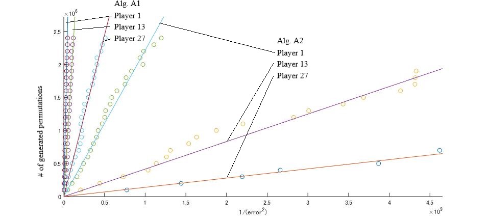
Figure 2: EU Council.

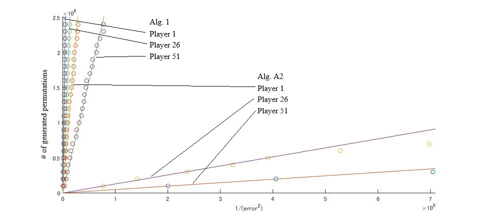
Figure 3: United States.

Table 2: Comparison of Algorithms A1 and A2.

EU Council	$\alpha$
	Alg. A1	Alg. A2	ratio
Player 1	0.0557	0.0022	25.318
Player 13	0.0199	$4.1615\times 10^{-4}$	47.819
Player 27	0.0049	$1.3987\times 10^{-4}$	35.033

United States	$\alpha$
	Alg. A1	Alg. A2	ratio
Player 1	0.0489	0.0181	2.7017
Player 26	0.0088	$1.2837\times 10^{-4}$	68.552
Player 51	0.0032	$4.8911\times 10^{-5}$	65.424

For each (generated) permutation, the computational effort of both Algorithms A1 and A2 are bounded by $\mbox{\rm O}(n)$. Here, we discuss the constant factors of $\mbox{\rm O}(n)$ computations. We tested the cases that weights $w_{i}$ are generated uniformly at random from the intervals $[1,10]$ or $[1,20]$, and quota is equal to $(1/2)\sum_{i\in N}w_{i}$. For each $n\in\{10,20,\ldots,100\}$, we executed Algorithms A1 and A2 by setting $M=10,000$. Under the assumption that computational time is equal to $an+b$, we estimated $a$ and $b$ by the least squares method. Figure 4 shows that for each permutation, the computational effort of Algorithm A2 increases about 5-fold comparing to Algorithm A1.

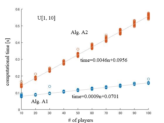
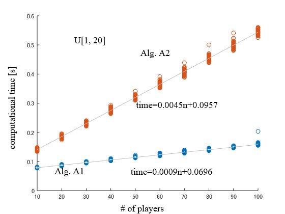
Figure 4: Computational time.

6 Conclusion

In this paper, we analyzed a naive Monte Carlo algorithm (Algorithm A1) for calculating the S-S index denoted by $(\varphi_{1},\varphi_{2},\ldots,\varphi_{n})$ in weighted majority games. By employing the Bretagnolle-Huber-Carol inequality [29] (Theorem 8 in Appendix), we estimated the required number of samples that gives an upper bound of the total variation distance.

We also proposed an efficient Monte Carlo algorithm (Algorithm A2). The time complexity of each iteration of our algorithm is equal to that of the naive algorithm (Algorithm A1). Our algorithm has the property that the obtained estimator $(\varphi^{\mbox{A2}}_{1},\varphi^{\mbox{A2}}_{2},\ldots,\varphi^{\mbox{A2}}_{n})$ satisfies

$$\mbox{ both }[\mbox{ if }\varphi_{i}<\varphi_{j}\mbox{ then }\varphi^{\mbox{A2}}_{i}\leq\varphi^{\mbox{A2}}_{j}]\mbox{ and }[\mbox{ if }\varphi_{i}=\varphi_{j}\mbox{ then }\varphi^{\mbox{A2}}_{i}=\varphi^{\mbox{A2}}_{j}].$$

We also proved that, even if we consider the property

$$\mbox{\rm Pr}\left[\forall i\in N,\left|\varphi^{\mbox{A2}}_{i}-\varphi_{i}\right|<\varepsilon\right]\geq 1-\delta,$$

the required number of samples is irrelevant to $n$ (the number of players).

APPENDIX (Bretagnolle-Huber-Carol inequality)

Theorem 8.

[29]

If the random vector $(Z_{1},Z_{2},\ldots,Z_{n})$ is multinomially distributed with parameters $(p_{1},p_{2},\ldots,p_{n})$ and satisfies $Z_{1}+Z_{2}+\cdots+Z_{n}=M$ then

$$\mbox{\rm Pr}\left[\sum_{i=1}^{n}\left|Z_{i}-Mp_{i}\right|\geq 2M\varepsilon\right]\leq 2^{n}\exp(-2M\varepsilon^{2}).$$

Proof. It is easy to see that

$$\mbox{\rm Pr}\left[\sum_{i=1}^{n}\left|Z_{i}-Mp_{i}\right|\geq 2M\varepsilon\right]=\mbox{\rm Pr}\left[2\max_{S\subseteq\{1,2,\ldots,n\}}\sum_{i\in S}(Z_{i}-Mp_{i})\geq 2M\varepsilon\right]$$

$$= \mbox{\rm Pr}\left[\exists S\subseteq\{1,2,\ldots,n\},\;\;\sum_{i\in S}(Z_{i}-Mp_{i})\geq M\varepsilon\right]\leq\sum_{S\subseteq\{1,2,\ldots,n\}}\mbox{\rm Pr}\left[\sum_{i\in S}(Z_{i}-Mp_{i})\geq M\varepsilon\right]$$

$$= \sum_{S\subseteq\{1,2,\ldots,n\}}\mbox{\rm Pr}\left[\sum_{i\in S}Z_{i}-M\sum_{i\in S}p_{i}\geq M\varepsilon\right]$$

For any subset $S\subseteq\{1,2,\ldots,n\}$, there exists a Bernoulli process $(X^{(1)}_{S},X^{(2)}_{S},\ldots,X^{(M)}_{S})$ satisfying $\sum_{i\in S}Z_{i}=\sum_{m=1}^{M}X^{(m)}_{S}$ and $\mbox{\rm E}[X^{(m)}_{S}]=\sum_{i\in S}p_{i}$ $(\forall m\in\{1,2,\ldots M\})$. Hoeffding’s inequality [14] implies that

$$\sum_{S\subseteq\{1,2,\ldots,n\}}\mbox{\rm Pr}\left[\sum_{i\in S}Z_{i}-M\sum_{i\in S}p_{i}\geq M\varepsilon\right]=\sum_{S\subseteq\{1,2,\ldots,n\}}\mbox{\rm Pr}\left[\sum_{m=1}^{M}X^{(m)}_{S}-\mbox{\rm E}\left[\sum_{m=1}^{M}X^{(m)}_{S}\right]\geq M\varepsilon\right]$$

$$= \sum_{S\subseteq\{1,2,\ldots,n\}}\mbox{\rm Pr}\left[\frac{1}{M}\sum_{m=1}^{M}X^{(m)}_{S}-\frac{1}{M}\mbox{\rm E}\left[\sum_{m=1}^{M}X^{(m)}_{S}\right]\geq\varepsilon\right]\leq\sum_{S\subseteq\{1,2,\ldots,n\}}\exp(-2M\varepsilon^{2})$$

$$= 2^{n}\exp(-2M\varepsilon^{2}).$$

QED

References

- [1] Bachrach, Y., Markakis, E., Resnick, E., Procaccia, A. D., Rosenschein, J. S., and Saberi, A. Approximating power indices: theoretical and empirical analysis. Autonomous Agents and Multi-Agent Systems, 20 (2010), 105–122.
- [2] Berghammer, R., Bolus, S., Rusinowska, A., and De Swart, H. A relation-algebraic approach to simple games. European Journal of Operational Research, 210 (2011), 68–80.
- [3] Bilbao, J. M., Fernandez, J. R., Losada, A. J., and Lopez, J. J. Generating functions for computing power indices efficiently. Top, 8 (2000), 191–213.
- [4] Bilbao, J. M., Fernandez, J. R., Jiménez, N., and Lopez, J. J. Voting power in the European Union enlargement. European Journal of Operational Research, 143 (2002), 181–196.
- [5] Bolus, S. Power indices of simple games and vector-weighted majority games by means of binary decision diagrams. European Journal of Operational Research, 210 (2011), 258–272.
- [6] Brams, S. J. and P. J. Affuso, P. J. Power and size; a new paradox. Mimeographed Paper, 1975.
- [7] Castro, J., Gómez, D., and Tejada, J. Polynomial calculation of the Shapley value based on sampling. Computers & Operations Research, 36 (2009), 1726–1730.
- [8] Castro, J., Gómez, D., Molina, E., and Tejada, J. Improving polynomial estimation of the Shapley value by stratified random sampling with optimum allocation. Computers & Operations Research, 82 (2017), 180–188.
- [9] Deng, X. and Papadimitriou, C. H. On the complexity of cooperative solution concepts. Mathematics of Operations Research, 19 (1994), 257–266.
- [10] Elkind, E., Goldberg, L. A., Goldberg, P., and Wooldridge, M. Computational complexity of weighted threshold games. In Proc. of the National Conference on Artificial Intelligence, AAAI Press, 718–723, 2007.
- [11] Fatima, S. S., Wooldridge, M., and Jennings, N. R. A linear approximation method for the Shapley value Artificial Intelligence, 172 (2008), 1673–1699.
- [12] Felsenthal, D. S. and Machover, M. The Treaty of Nice and qualified majority voting. Social Choice and Welfare, 18 (2001), 431–464.
- [13] Garey, M. R. and Johnson, D. S. Computers and Intractability: A Guide to the Theory of NP-Completeness. WH Freeman, 1979.
- [14] Hoeffding, W. Probability inequalities for sums of bounded random variables, Journal of the American Statistical Association, 58 (1963), 13–30.
- [15] Klinz, B. and Woeginger, G. J. Faster algorithms for computing power indices in weighted voting games. Mathematical Social Sciences, 49 (2005), 111–116.
- [16] Leech, D. Computing power indices for large voting games. Management Science, 49 (2003), 831–837.
- [17] Lucas, W. F. Measuring power in weighted voting systems. Brams, S. J., Lucas, W. F., and Straffin, P. D. (eds.): Political and Related Models, Springer, 183–238, 1983.
- [18] Mann, I. and Shapley, L. S. Values of large games. IV: evaluating the electoral college by Montecarlo techniques. Technical Report, The RAND Corporation, RM-2651, 1960.
- [19] Mann, I. and Shapley, L. S. Values of large games. VI: Evaluating the electoral college exactly. Technical Report, The RAND Corporation, RM-3158-PR, 1962.
- [20] Matsui, T. and Matsui, Y. A survey of algorithms for calculating power indices of weighted majority games. Journal of the Operations Research Society of Japan, 43 (2000), 71–86.
- [21] Matsui, Y. and Matsui, T. NP-completeness for calculating power indices of weighted majority games. Theoretical Computer Science, 263 (2001), 305–310.
- [22] Owen, G. Multilinear extensions of games. Management Science, 18 (1972), 64–79.
- [23] Owen, G. Game Theory. Academic press, 1995.
- [24] Prasad, K. and Kelly, J. S. NP-completeness of some problems concerning voting games. International Journal of Game Theory, 19 (1990), 1–9.
- [25] Rushdi, A. M. A. and Ba-Rukab, O. M. Map calculation of the Shapley-Shubik voting powers: An example of the European Economic Community. International Journal of Mathematical, Engineering and Management Sciences (IJMEMS), 2 (2017), 17–29.
- [26] Shapley, L. S. A value for -person games. Kuhn, H. W. and Tucker, A. W. Tucker (eds.), Contributions to the Theory of Games II, Princeton University Press, 307–317, 1953.
- [27] Shapley, L. S. and Shubik, M. An algorithm for evaluating the distribution of power in a committee system. American Political Science Review, 48 (1954), 787–792.
- [28] Uno, T. Efficient computation of power indices for weighted majority games. In Proc. of International Symposium on Algorithms and Computation (ISAAC), LNCS 7676, Springer, 679–689, 2012.
- [29] van der Vaart, A. W. and Wellner, J. A. Weak Convergence and Empirical Processes: with Applications to Statistics, Springer, 1989.
- [30] von Neumann, J. and Morgenstern, O. Theory of Games and Economic Behavior. Princeton Univ. Press, 1944.