Shallow Bayesian Meta Learning for Real-World Few-Shot Recognition

Abstract

Many state-of-the-art few-shot learners focus on developing effective training procedures for feature representations, before using simple (e.g., nearest centroid) classifiers. We take an approach that is agnostic to the features used, and focus exclusively on meta-learning the final classifier layer. Specifically, we introduce MetaQDA, a Bayesian meta-learning generalisation of the classic quadratic discriminant analysis. This approach has several benefits of interest to practitioners: meta-learning is fast and memory efficient, without the need to fine-tune features. It is agnostic to the off-the-shelf features chosen, and thus will continue to benefit from future advances in feature representations. Empirically, it leads to excellent performance in cross-domain few-shot learning, class-incremental few-shot learning, and crucially for real-world applications, the Bayesian formulation leads to state-of-the-art uncertainty calibration in predictions.

1 Introduction

Few-shot recognition methods aim to solve classification problems with limited labelled training data, motivating a large body of work [62]. Contemporary approaches to few-shot recognition are characterized by a focus on deep meta-learning [23] methods that provide data efficient learning of new categories by using auxiliary data to train a model designed for rapid adaptation to new categories [8, 69], or for synthesizing a classifier for new categories in a feed-forward manner [38, 43]. Most of these meta-learning methods have been intimately interwoven with the training algorithm and/or architecture of the deep network that they build upon. For example, many have relied on episodic training schemes [52, 59], where few-shot learning problems are simulated at each iteration of training; differentiable optimisers [3, 30], or new neural network modules [55, 15] to facilitate data efficient learning and recognition.

Against this backdrop, a handful of recent studies [61, 14, 4, 37, 64, 60] have pushed back against deep meta-learning. They have observed, for example, that a well tuned convolutional network pre-trained for multi-class recognition and combined with a simple linear or nearest centroid classifier can match or outperform state-of-the-art meta-learners. Even self-supervised pre-training [37] has led to feature extractors that outperform many meta-learners. These analyses raise the question: is meta-learning indeed beneficial, or is focusing on improving conventional pre-training sufficient?

We take a position in defense of meta-learning for few-shot recognition. To disentangle the influences of meta-learning per-se and feature learning discussed above, we restrict ourselves to fixed pre-trained features and conduct no feature learning in this study. It shows that meta-learning, even in its shallowest form, can boost few-shot learning above and beyond whatever is provided by the pre-trained features alone.

We take an amortized Bayesian inference approach [15, 21] to shallow meta-learning. During meta-testing, we infer a distribution over classifier parameters given the support set; and during meta-training we learn a feed-forward inference procedure for these parameters. While the limited recent work in Bayesian meta-learning is underpinned by amortized Variational Inference [15], our approach relies instead on conjugacy [12]. Specifically, we build upon the classic Quadratic Discriminant Analysis (QDA) [9] classifier and extended it with a Bayesian prior, an inference pipeline for the QDA parameter posterior given the support set, and gradient-based meta-training. We term the overall framework MetaQDA.

MetaQDA has several practical benefits for real-world deployments. Firstly, MetaQDA allows meta-learning to be conducted in the resource constrained scenario without end-to-end training [24], while providing superior performance to fixed-feature approaches [61, 4, 37]. Furthermore by decomposing representation learning from classifier meta-learning, MetaQDA is expected to benefit from continued progress in CNN architectures and training strategies. Indeed our empirical results show our feature-agnostic strategy benefits a diverse range of classic and recent feature representations.

Secondly, as computer vision systems begin to be deployed in high-consequence applications where safety [28] or fair societal outcomes [5] are at stake, their calibration becomes as equally, or more, important as their actual accuracy. E.g., Models must reliably report low-certainty in those cases where they do make mistakes, thus allowing their decisions in those cases to be reviewed. Indeed, proper calibration is a hard requirement for deployment in many high importance applications [17, 40]. Crucially, we show that our Bayesian MetaQDA leads to significantly better calibrated models than the standard classifiers in the literature.

Finally, we show that MetaQDA has particularly good performance in cross-domain scenarios where existing methods are weak [4], but which are ubiquitious in practical applications, where there is invariably insufficient domain-specific data to conduct in-domain meta-learning [18]. Furthermore, as a Bayesian formulation, MetaQDA is inherently suited to the highly practical, but otherwise hard to achieve setting of incremental [56, 45] few-shot learning, where it achieves state of the art performance ‘out of the box’.

To summarize our contributions: (i) We present MetaQDA, a novel and efficient Bayesian approach to classifier meta-learning based on conjugacy. (ii) We empirically demonstrate that MetaQDA’s efficient fixed feature learning provides excellent performance across a variety of settings and metrics including conventional, cross-domain, class-incremental, and probability calibrated few-shot learning. (iii) We shed light on the meta-learning vs vanilla pre-training debate by disentangling the two and showing a clear benefit from meta-learning, across a variety of fixed feature representations.

2 Related Work

Few-Shot and Meta-Learning Overview  Few-shot and meta-learning are now a widely studied area that is too broad to review here. We refer the reader to comprehensive recent surveys for an introduction and review [62, 23]. In general they proceed in two stages: meta-training the strategy for few-shot learning based on one or more auxiliary datasets; and meta-testing (learning new categories) on a target dataset, which should be done data-efficiently given the knowledge from meta-training. A high level categorization of common approaches groups them into methods that (1) meta-learn how to perform rapid gradient-based adaptation during meta-test [8, 69]; and (2) meta-learn a feed-forward procedure to synthesize a classifier for novel categories given an embedding of the support set [15, 43], where metric-based learners are included in the latter category [23].

Is Meta-Learning Necessary?  Many recent papers have questioned whether elaborate meta-learning procedures are necessary. SimpleShot [61] observes vanilla CNN features pre-trained for recognition achieve near SotA performance when appropriately normalized and used in a trivial nearest centroid classifier (NCC). Chen et al. [4] present the simple but high-performance Baseline++, based on fixing a pre-trained feature extractor and then building a linear classifier during meta-test. [14] observe that although SotA meta-learned deep features do exhibit strong performance in few-shot learning, this feature quality can be replicated by adding simple compactness regularisers to vanilla classifier pre-training. S2M2 [37] demonstrates that after pre-training a network with self-supervised learning and/or manifold-regularised vanilla classification, excellent few-shot recognition is achieved by simply training a linear classifier on the resulting representation. [64] analyzes whether the famous MAML algorithm is truly meta-learning, or simply pre-training a strong feature.

We show that for fixed features pre-trained by several of the aforementioned “off-the-shelf” non-meta techniques [61, 37], meta-learning solely in classifier-space further improves performance. This allows us to conclude that meta-learning does add value, since alternative vanilla (i.e., non-meta) pre-training approaches do not influence the final classifier. We leave conclusive analysis of the relative merits of meta-learning vs vanilla pre-training of feature representation space to future work. In terms of empirical performance, we surpass all existing strategies based on fixed pre-trained features, and most alternatives based on deep feature meta-learning.

Fixed Feature Meta-Learning  A minority of meta-learning studies such as [50, 34] have also built on fixed features. LEO [50] synthesizes a classifier layer for a fixed feature extractor using a hybrid gradient- and feedforward-strategy. The concurrent URT [34] addresses multi-domain few-shot learning by meta-training a module that fuses an array of fixed features and dynamically produces a new feature encoding for a new domain. Ultimately, URT uses a ProtoNet [52] classifier, and thus our contribution is orthogonal to URT’s, as MetaQDA aims to replace the classifier (ie, ProtoNet), not produce a new feature. Indeed we show empirically that MetaQDA can use URT’s feature and improve their performance, further demonstrating the flexibility of our feature-agnostic approach.

Bayesian Few-Shot Meta-Learning  Relatively few methods in the literature take Bayesian approaches to few-shot learning. A few studies [16, 65] focus on understanding MAML [8] as a hierarchical Bayesian model. Versa [15] treats the weights of the final linear classifier layer as the quantity to infer given the support set during meta-test. It takes an amortized variational inference (VI) approach, training an inference neural network to predict the classifier parameters given the support set. However, unlike us, it then performs end-to-end representation learning, and is not fully Bayesian as it does not ultimately integrate the classifier parameters, as we achieve here. Neural Processes [11] takes a Gaussian Process (GP) inspired approach to neural network design, but ultimately does not provide a clear Bayesian model. The recent DKT [42] achieves true Bayesian meta-learning via GPs with end-to-end feature learning. However, despite performing feature learning, these Bayesian approaches have generally not provided SotA benchmark performance compared to the broader landscape of competitors at the time of their publication. A classic study [21] explored shallow learning-to-learn of linear regression by conjugacy. We also exploit conjugacy but for classifier learning, and demonstrate SotA results on heavily benchmarked tasks for the first time with Bayesian meta-learning.

Classifier Layer Design  The vast majority of few-shot studies use either linear [37, 15, 7], cosine similarity [43], or nearest centroid classifiers [61, 52] under some distance metric. We differ in: (i) using a quadratic classifier, and (ii) taking a “generative” approach to fitting the model [19]. While a quadratic classifier potentially provides a stronger fit than a linear classifier, its larger number of parameters will overfit catastrophically in a few-shot/high-dimension regime. This is why few studies have applied them, with the exception of [1] who had to carefully hand-craft regularisers for them. Our key insight is to use conjugacy to enable the quadratic classifier prior to be efficiently meta-learned, thus gaining improved fitting strength, while avoiding overfitting.

3 Probabilistic Meta-Learning

One can formalise a conventional classification problem as consisting of an input space $\mathcal{X}$, an output space $\mathcal{Y}$, and a distribution $p$ over $\mathcal{X}\times\mathcal{Y}$ that defines the task to be solved. Few-shot recognition is the problem of training a classifier to distinguish between $C$ different classes in a sparse data regime, where only $K$ labelled training instances are available for each class. Meta-learning aims to distill relevant knowledge from multiple related few-shot learning problems into a set of shared parameters that boost the learning of subsequent novel few-shot tasks. The simplest way to extend the standard formalisation of classification problems to a meta-learning context is to instead consider the set, $\mathcal{P}$ of all distributions over $\mathcal{X}\times\mathcal{Y}$, each of which represents a possible classification task. One can then assume the existence of a distribution, $Q$ over $\mathcal{P}$ [2].

From a probabilistic perspective, the parameters inferred by the meta-learner that are shared across tasks, which we denote by $\phi$, can be seen as specifying or inducing a prior distribution over the task-specific parameters for each few-shot problem. As such, meta-learning can be thought of as learning a procedure to induce a prior over models for future tasks by meta-training on a collection of related tasks. Representing task-specific parameters for task $t$ by $\theta_{t}$, the few-shot training (aka support) and testing (aka query) sets as $D_{S}^{t}$ and $D^{t}_{Q}$, a Bayesian few-shot learner should use the learned prior to determine the posterior distribution over model parameters,

$$p(\theta_{t}|D_{S}^{t},\phi)=\frac{p(D_{S}^{t}|\theta_{t})p(\theta_{t}|\phi)}{\int p(D_{S}^{t}|\theta_{t})p(\theta_{t}|\phi)\textup{d}\theta_{t}}.$$ (1)

Once the distribution obtained, one can model query samples, $(\vec{x}_{i}^{t},y_{i}^{t})\in D_{Q}^{t}$, using the posterior predictive distribution,

$$p(D_{Q}^{t}|D_{S}^{t},\phi)=\prod_{i=1}^{|D_{Q}^{t}|}\int p(\vec{x}_{i}^{t},y_{i}^{t}|\theta_{t})p(\theta_{t}|D_{S}^{t},\phi)\textup{d}\theta_{t}.$$ (2)

A natural measure for the goodness of fit for $\phi$ is the expected log likelihood of the few-shot models that make use of the shared prior,

$$\underset{D_{S},D_{Q}\sim q,q\sim Q}{\mathbb{E}}[L(\phi|D_{S},D_{Q})],$$ (3)

where

$$L(\phi|D_{S},D_{Q})=\sum_{i=1}^{|D_{Q}|}\textup{log}\,p(\vec{x}_{i},y_{i}|D_{S},\phi).$$ (4)

The process of meta-learning the prior parameters can then be formalised as an risk minimisation problem,

$$\phi^{\ast}=\operatorname*{arg\,min}_{\phi}\underset{D_{S},D_{Q}\sim q,q\sim Q}{\mathbb{E}}[-L(\phi|D_{S},D_{Q})].$$ (5)

Discussion  A prior probabilistic meta-learner [15] focused on the term $p(\theta_{t}|D_{S}^{t},\phi)$, taking an amortized variational inference perspective that treats $\phi$ as the parameters of a neural network that predicts a distribution over the parameters $\theta_{t}$ of a linear classifier given support set $D_{S}^{t}$. In contrast, our framework will use a QDA rather than linear classifier, and then exploit conjugacy to efficiently compute a distribution over the QDA mean and covariance parameters $\theta_{t}$ given the support set. This is both efficient and probabilistically cleaner, as our model contains a proper prior, while [15] does not.

The integrals in Eqs. 1 and 2 are key to Bayesian meta-learning, but can be computationally intractable and [15] relies on sampling. Our conjugate setup allows the integrals to be computed exactly in closed form, without relying on sampling.

4 Meta-Quadratic Discriminant Analysis

Our MetaQDA provides a meta-learning generalization of the classic QDA classifier [19]. QDA works by constructing a multivariate Gaussian distribution $\theta$ corresponding to each class by maximum likelihood. At test time, predictions are made by computing the likelihood of the query instance under each of these distributions, and using Bayes theorem to obtain the posterior $p(y|x,\theta)$. Rather than using maximum likelihood fitting for meta-testing, we introduce a Bayesian version of QDA that will enable us to exploit a meta-learned prior over the parameters of the multivariate Gaussian distributions. Two Bayesian strategies for inference using such a prior are explored: 1) using the maximum a posterior (MAP) estimate of the Gaussian parameters; and 2) the fully Bayesian approach that propagates the parameter uncertainty through to the class predictions. The first of these is conceptually simpler, while the second allows for better handling of uncertainty due to the fully Bayesian nature of the parameter inference. For both cases we make use of Normal-Inverse-Wishart priors [12], as their conjugacy with multivariate Gaussians leads to an efficient implementation strategy.

4.1 MAP-Based QDA

We begin by describing a MAP variant of QDA. In conventional QDA the likelihood of an instance, $\vec{x}\in\mathbb{R}^{d}$, belonging to class $j\in\mathbb{N}_{C}$ is given by $\mathcal{N}(\vec{x}|\vec{\mu}_{j},\Sigma_{j})$ and the parameters are found via maximum likelihood estimation (MLE) on the subset of the support set associated with class $j$,

$$\vec{\mu}_{j},\Sigma_{j}=\operatorname*{arg\,max}_{\vec{\mu},\Sigma}\prod_{i=1}^{K}\mathcal{N}(\vec{x}_{j,i}|\vec{\mu},\Sigma).$$ (6)

This optimisation problem has a convenient closed form solution: the sample mean and covariance of the relevant subset of the support set. In order to incorporate prior knowledge learned from related few-shot learning tasks, we define a Normal-inverse-Wishart (NIW) prior [39] over the parameters and therefore obtain a posterior for the parameters,

$$\begin{split}&p(\vec{\mu}_{j},\Sigma_{j}|\vec{x},\vec{m},\kappa,S,\nu)\\ &=\frac{\prod_{i=1}^{K}\mathcal{N}(\vec{x}_{j,i}|\vec{\mu}_{j},\Sigma_{j})\mathcal{NIW}(\vec{\mu}_{j},\Sigma_{j}|\vec{m},\kappa,S,\nu)}{\int\int\prod_{i=1}^{K}\mathcal{N}(\vec{x}_{j,i}|\vec{\mu},\Sigma)\mathcal{NIW}(\vec{\mu}^{\prime},\Sigma^{\prime}|\vec{m},\kappa,S,\nu)d\vec{\mu}^{\prime}d\Sigma^{\prime}}.\end{split}$$ (7)

Training  This enables us to take advantage of prior knowledge learned from related tasks when inferring the model parameters by MAP inference,

$$\vec{\mu}_{j},\Sigma_{j}=\operatorname*{arg\,max}_{\vec{\mu},\Sigma}\prod_{i=1}^{K}p(\vec{\mu}_{j},\Sigma_{j}|\vec{x}_{j,i},\vec{m},\kappa,S,\nu).$$ (8)

Because NIW is the conjugate prior of multivariate Gaussians, we know that the posterior distribution over the parameters takes the form of

$$p(\vec{\mu}_{j},\Sigma_{j}|\vec{x},\vec{m},\kappa,S,\nu)=\mathcal{NIW}(\vec{\mu}_{j},\Sigma_{j}|\vec{m}_{j},\kappa_{j},S_{j},\nu_{j}),$$ (9)

where

$$\begin{split}\vec{m}_{j}&=\frac{\vec{m}+K\hat{\vec{\mu}}_{j}}{\kappa+K},\quad\kappa_{j}=\kappa+K,\quad\nu_{j}=\nu+K,\\ S_{j}&=S+\sum_{i=1}^{K}(\vec{x}_{j,i}-\hat{\vec{\mu}}_{j})(\vec{x}_{j,i}-\hat{\vec{\mu}}_{j})^{T}+\\ &\quad\frac{\kappa K}{\kappa+K}(\hat{\vec{\mu}}_{j}-\vec{m})(\hat{\vec{\mu}}_{j}-\vec{m})^{T},\end{split}$$ (10)

and we have used $\hat{\vec{\mu}}_{j}=\frac{1}{k}\sum_{i=1}^{K}\vec{x}_{j,i}$. The posterior is maximised at the mode, which occurs at

$$\vec{\mu}_{j}=\vec{m}_{j},\quad\Sigma_{j}=\frac{1}{\nu_{j}+d+1}S_{j}.$$ (11)

Testing  After computing point estimates of the parameters, one can make predictions on instances from the query set according to the usual QDA model,

$$p(y=j|\vec{x},\vec{m},\kappa,S,\nu)=\frac{\mathcal{N}(\vec{x}|\vec{\mu}_{j},\Sigma_{j})p(y=j)}{\sum_{i=1}^{C}\mathcal{N}(\vec{x}|\vec{\mu}_{i},\Sigma_{i})p(y=i)}.$$ (12)

Note the prior over the classes $p(y)$ can be dropped in the standard few-shot benchmarks that assume a uniform distribution over classes.

4.2 Fully Bayesian QDA

Computing point estimates of the parameters throws away potentially useful uncertainty information that can help to better calibrate the predictions of the model. Instead, we can marginalise the parameters out when making a prediction,

$$\begin{split}&p(y=j|\vec{x})\\ &=\frac{\int\int\mathcal{N}(\vec{x}|\mu_{j},\Sigma_{j})\mathcal{NIW}(\vec{\mu}_{j},\Sigma_{j}|\vec{m}_{j},\kappa_{j},S_{j},\nu_{j})d\vec{\mu}_{j}d\Sigma_{j}}{\sum_{i=1}^{C}\int\int\mathcal{N}(\vec{x}|\mu_{i},\Sigma_{i})\mathcal{NIW}(\vec{\mu}_{i},\Sigma_{i}|\vec{m}_{j},\kappa_{j},S_{j},\nu_{j})d\vec{\mu}_{i}d\Sigma_{i}}.\end{split}$$ (13)

Each of the double integrals has the form of a multivariate $t$-distribution [39], yielding

$$\begin{split}&p(y=j|\vec{x},\vec{m},\kappa,S,\nu)\\ &=\frac{\mathcal{T}\Big{(}\vec{x}|\vec{m}_{j},\frac{\kappa_{j}+1}{\kappa_{j}(\nu_{j}-d+1)}S_{j},\nu_{j}-d+1\Big{)}}{\sum_{i=1}^{C}\mathcal{T}\Big{(}\vec{x}|\vec{m}_{i},\frac{\kappa_{i}+1}{\kappa_{i}(\nu_{i}-d+1)}S_{i},\nu_{i}-d+1\Big{)}}.\end{split}$$ (14)

4.3 Meta-Learning the Prior

Letting $\phi=(\vec{m},\kappa,S,\nu)$, our objective is to minimise the negative expected log likelihood of models constructed with the shared prior on the parameters, as given in Eq. 5. For MAP-based QDA, the log likelihood function is given by

$$L(\phi|D_{S},D_{Q})=\sum_{j=1}^{C}\sum_{i=1}^{K}\textup{log}\,\mathcal{N}(\vec{x}_{j,i}|\vec{\mu}_{j},\Sigma_{j}),$$ (15)

where $\vec{\mu}_{j}$ and $\Sigma_{j}$ are the point estimates computed via the closed-form solution to the MAP inference problem given in Equation 11. When using the fully Bayesian variant of QDA, we have the following log likelihood function:

$$\begin{split}&L(\phi|D_{S},D_{Q})\\ &=\sum_{j=1}^{C}\sum_{i=1}^{K}\textup{log}\,\mathcal{T}\Big{(}\vec{x}_{j,i}|\vec{m}_{j},\frac{\kappa_{j}+1}{\kappa_{j}(\nu_{j}-d+1)}S_{j},\nu_{j}-d+1\Big{)}.\end{split}$$ (16)

Meta-Training  We approximate the optimization in Equation 5 by performing empirical risk minimisation on a training dataset using episodic training. In particular, we choose $\mathcal{P}$ to be the set of uniform distributions over all possible $C$-way classification problems, $Q$ as the uniform distribution over $\mathcal{P}$, and the process of sampling from each $q\in\mathcal{P}$ results in balanced datasets containing $K$ instances from each of the $C$ classes. Episodic training then consists of sampling a few-shot learning problem, building a Bayesian QDA classifier using the support set, computing the negative log likelihood on the query set, and finally updating $\phi$ using stochastic gradient descent. Crucially, the use of conjugate priors means that no iterative optimisation procedure must be carried out when constructing the classifier in each episode. Instead, we are able to backpropagate through the conjugacy update rules and directly modify the prior parameters with stochastic gradient descent. The overall learning procedure is given in Algorithm 1.

Some of the prior parameters must be constrained in order to learn a valid NIW distribution. In particular, $S$ must be positive definite, $\kappa$ must be positive, and $\nu$ must be strictly greater than $d-1$. The constraints can be enforced for $\kappa$ and $\nu$ by clipping any values that are outside the valid range back to the minimum allowable value. We parameterise the scale matrix in terms of its Cholesky factors,

$$S=LL^{T},$$ (17)

where $L$ is a lower triangular matrix. During optimisation we ensure $L$ remains lower triangular by setting all elements above the diagonal to zero after each weight update.

1 Require: Distribution over tasks $Q$, number of iterations $T$, learning rate $\alpha$

2 Result: prior parameters $\phi_{T}$

3 Init: $\phi_{0}=\{\vec{m}=\vec{0},S=\mathbb{I},\kappa=1,\nu=d\}$

4 for $t=1\textup{ to }T$ do

5       Sample task, $q_{t}\sim Q$ ;

6       Sample support and query set, $D_{S}^{t},D_{Q}^{t}\sim q_{t}$ ;

7       Build Bayesian QDA Model

       If MAP: $\theta_{t}\leftarrow\{(\vec{\mu}_{j},\Sigma_{j})\}_{j=1}^{C}$ ;

        // Eq 11

       If Fully Bayes: $\theta_{t}\leftarrow\{(\vec{m}_{j},\kappa_{j},S_{j},\nu_{j})\}_{j=1}^{C}$ ;

        // Eq 10

8       Update Prior

       $\phi_{t}\leftarrow\phi_{t-1}-\alpha\nabla_{\phi}L(\phi_{t-1}|D_{S}^{t},D_{Q}^{t})$ ;

        // Eq 15 or LABEL:eq:full-likelihood

9      

10 end for

Algorithm 1 Pseudocode for epsiodic meta-learning of hyper-parameters in MetaQDA.

5 Experiments

We measure the efficacy of our model in standard, cross-domain and multi-domain few-shot learning and few-shot class-incremental problem settings. MetaQDA is a shallow classifier-layer meta-learner that is agnostic to the choice of fixed extracted features. Unless otherwise stated, we report results for the FB-based variant of MetaQDA. During meta-training, we learn the priors $\phi=(\vec{m},\kappa,S,\nu)$ over episodes drawn from the training set, keeping the feature extractor fixed. We use the meta-validation datasets for model selection and hyperparameter tuning. During meta-testing, the support set is used to obtain the parameter posterior, and then a QDA classifier is established according to either Eq 12 or Eq 14. All algorithms are evaluated on $C$-way $k$-shot learning [52], with a batch of 15 query images per class in a testing episode. All accuracies are calculated by averaging over 600 randomly generated testing tasks with 95% confidence interval.

5.1 Standard Few-Shot Learning

Datasets  miniImageNet [44] is split into 64/16/20 for meta-train/val/test, respectively, containing 100 classes and 600 examples per class, drawn from ILSVRC-12 [49]. Images are resized to 84$\times$84 [20]. tieredImageNet is a more challenging benchmark [47] consisting of 608 classes (779,165 images) and 391/97/160 classes for meta-train/val/test folds, respectively. Images are resized to 84$\times$84. CIFAR-FS [3] was created by randomly sampling from CIFAR-100 [27] by using the same criteria as miniImageNet (100 classes with 600 images per class, split into folds of 64/16/20 for meta-train/val/test). Image are resized to 32$\times$32.

Feature Extractors  Conv-4 (64-64-64-64) as in [52]. See Appendix for details. ResNet-18 is standard 18-layer 8-block architecture with pre-trained weights in [61]. WRN-28-10 is standard architecture with 28 convolutional layers and width factor 10, and the pre-trained weights from [37].

Competitors  We group competitors into two categories: 1) direct competitors that also make use of “off-the-shelf” fixed pre-trained networks and only update the classifier to learn novel classes; and 2) non-direct competitors that specifically meta-learn a feature optimised for few-shot learning and/or update features during meta-testing. Baseline++ [4] fixes the feature encoder and only tunes the (cosine similarity) classifier during the meta-test stage. SimpleShot [61] uses an NCC classifier with different feature encoders and studies different feature normalizations. We use their best reported variant, CL2N. S2M2 [37] uses a linear classifier after self-supervised and/or regularized classifier pre-training. SUR [7] also uses pre-trained feature extractors, but focuses on weighting multiple features extracted from different backbones or multiple layers of the same backbone. We compare their reported results of a single ResNet backbone trained for multi-class classification as per ours, but they have the advantage of fusing features extracted from multiple layers. Unravelling [14] proposes some new regularizers for vanilla backbone training that improve feature quality for few-shot learning without meta-learning.

Model	Backbone	1-shot	5-shot
MetaLSTM [44]	Conv-4	43.44 $\pm$ 0.77%	60.60 $\pm$ 0.71%
MAMLO [8]	Conv-4	48.70 $\pm$ 1.84%	63.11 $\pm$ 0.92%
ProtoNet [52]	Conv-4	49.42 $\pm$ 0.78%	68.20 $\pm$ 0.66%
GNN [10]	Conv-4	50.33 $\pm$ 0.36%	66.41 $\pm$ 0.63%
MetaSSL[47]	Conv-4	50.41 $\pm$ 0.31%	64.39 $\pm$ 0.24%
RelationNet [55]	Conv-4	50.44 $\pm$ 0.82%	65.32 $\pm$ 0.70%
MetaSGDO [33]	Conv-4	50.47 $\pm$ 1.87%	64.03 $\pm$ 0.94%
CAVIA [69]	Conv-4	51.82 $\pm$ 0.65%	65.85 $\pm$ 0.55%
TPN [35]	Conv-4	52.78 $\pm$ 0.27%	66.59 $\pm$ 0.28%
R2D2 [3]	Conv-4∗	51.90 $\pm$ 0.20%	68.70 $\pm$ 0.20%
RelationNet2[68]	Conv-4	53.48 $\pm$ 0.78%	67.63 $\pm$ 0.59%
GCR [31]	Conv-4	53.21 $\pm$ 0.40%	72.34 $\pm$ 0.32%
VERSA [15]	Conv-4	53.40 $\pm$ 1.82%	67.37 $\pm$ 0.86%
DynamicFSL† [13]	Conv-4	56.20 $\pm$ 0.86%	72.81 $\pm$ 0.62%
Baseline++ [4]	Conv-4	48.24 $\pm$ 0.75%	66.43 $\pm$ 0.63%
SimpleShot[61]	Conv-4	49.69 $\pm$ 0.19%	66.92 $\pm$ 0.17%
MetaQDA	Conv-4	56.41 $\pm$ 0.80%	72.64 $\pm$ 0.62%
SNAIL [51]	ResNet-12	55.71 $\pm$ 0.99%	68.88 $\pm$ 0.92%
Dynamic FSL [13]	ResNet-12	55.45 $\pm$ 0.89%	70.13 $\pm$ 0.68%
TADAM [41]	ResNet-12	58.50 $\pm$ 0.30%	76.70 $\pm$ 0.30%
CAML [25]	ResNet-12	59.23 $\pm$ 0.99%	72.35 $\pm$ 0.18%
AM3 [63]	ResNet-12	65.21 $\pm$ 0.49%	75.20 $\pm$ 0.36%
MTL [54]	ResNet-12∗	61.20 $\pm$ 1.80%	75.50 $\pm$ 0.80%
Tap Net [66]	ResNet-12	61.65 $\pm$ 0.15%	76.36 $\pm$ 0.10%
RelationNet2[68]	ResNet-12	63.92 $\pm$ 0.98%	77.15 $\pm$ 0.59%
R2D2[3]	ResNet-12	59.38 $\pm$ 0.31%	78.15 $\pm$ 0.24%
MetaOptO [30]	ResNet-12∗	64.09 $\pm$ 0.62%	80.00 $\pm$ 0.45%
RelationNet [4]	ResNet-18	52.48 $\pm$ 0.86%	69.83 $\pm$ 0.68%
ProtoNet [4]	ResNet-18	54.16 $\pm$ 0.82%	73.68 $\pm$ 0.65%
DCEM [6]	ResNet-18	58.71 $\pm$ 0.62%	77.28 $\pm$ 0.46%
AFHN [32]	ResNet-18	62.38 $\pm$ 0.72%	78.16 $\pm$ 0.56%
SUR[7]	ResNet-12	60.79 $\pm$ 0.62%	79.25 $\pm$ 0.41%
Unravelling[14]	ResNet-12∗	59.37 $\pm$ 0.32%	77.05 $\pm$ 0.25%
Baseline++ [4]	ResNet-18	51.87 $\pm$ 0.77%	75.68 $\pm$ 0.63%
SimpleShot[61]	ResNet-18	62.85 $\pm$ 0.20%	80.02 $\pm$ 0.14%
S2M2 [37]	ResNet-18	64.06 $\pm$ 0.18%	80.58 $\pm$ 0.12%
MetaQDA	ResNet-18	65.12 $\pm$ 0.66%	80.98 $\pm$ 0.75%
LEOO [50]	WRN	61.78 $\pm$ 0.05%	77.59 $\pm$ 0.12%
PPA [43]	WRN	59.60 $\pm$ 0.41%	73.74 $\pm$ 0.19%
SimpleShot[61]	WRN	63.50 $\pm$ 0.20%	80.33 $\pm$ 0.14%
S2M2 [37]	WRN	64.93 $\pm$ 0.18%	83.18 $\pm$ 0.22%
MetaQDA	WRN	67.83 $\pm$ 0.64%	84.28 $\pm$ 0.69%

Table 1: Few-shot classification results on miniImageNet. ^†: two-step optimization with attention. ^O: requires gradient-based optimisation at meta-test time. ^∗: Use a wider CNN than standard and higher dimensional embedding. Grey: Fixed feature methods.

Results  Table 1-3 summarize the results on miniImageNet, tieredImageNet and CIFAR-FS. MetaQDA performs better than all the previous methods that rely on off-the-shelf feature extractors, and also the majority of methods that meta-learn representations specialised for few-shot problems. We do not make efforts to carefully fine-tune the hyperparameters, but focus on showing that our model has robust advantages in different few-shot learning benchmarks with various backbones. A key benefit of fixed feature approaches (grey) is small compute cost, e.g., under 1-hour training. In contrast, SotA end-to-end competitors (white) such as [30, 13, 68] require over 10 hours.

Model	Backbone	1-shot	5-shot
MAML [35]	Conv-4	51.67 $\pm$ 1.81%	70.30 $\pm$ 1.75%
MetaSSL† [47]	Conv-4	52.39 $\pm$ 0.44%	70.25 $\pm$ 0.31%
RelationNet [35]	Conv-4	54.48 $\pm$ 0.48%	71.31 $\pm$ 0.78%
TPN† [35]	Conv-4	59.91 $\pm$ 0.94%	73.30 $\pm$ 0.75%
RelationNet2[68]	Conv-4	60.58 $\pm$ 0.72%	72.42 $\pm$ 0.69%
ProtoNet [35]	Conv-4	53.31 $\pm$ 0.89%	72.69 $\pm$ 0.74%
SimpleShot[61]	Conv-4	51.02 $\pm$ 0.20%	68.98 $\pm$ 0.18%
MetaQDA	Conv-4	58.11 $\pm$ 0.48%	74.28 $\pm$ 0.73%
TapNet [66]	ResNet-12	63.08 $\pm$ 0.15%	80.26 $\pm$ 0.12%
RelationNet2 [68]	ResNet-12	68.58 $\pm$ 0.63%	80.65 $\pm$ 0.91%
MetaOptNetO [30]	ResNet-12∗	65.81 $\pm$ 0.74%	81.75 $\pm$ 0.53%
SimpleShot [61]	ResNet-18	69.09 $\pm$ 0.22%	84.58 $\pm$ 0.16%
MetaQDA	ResNet-18	69.97 $\pm$ 0.52%	85.51 $\pm$ 0.58%
LEO [50]	WRN	66.33 $\pm$ 0.05%	81.44 $\pm$ 0.09%
SimpleShot [61]	WRN	69.75 $\pm$ 0.20%	85.31 $\pm$ 0.15%
S2M2 [37]	WRN	73.71 $\pm$ 0.22%	88.59 $\pm$ 0.14%
MetaQDA	WRN	74.33 $\pm$ 0.65%	89.56 $\pm$ 0.79%

Table 2: Few-shot classification results on tieredImageNet. ^†: Make use of additional unlabeled data for semi-supervised learning or transductive inference. Gray: Use fixed pre-trained backbones.

Model	Backbone	1-shot	5-shot
MAML [37]	Conv-4	58.90 $\pm$ 1.90%	71.50 $\pm$ 1.00%
RelationNet [37]	Conv-4	55.50 $\pm$ 1.00%	69.30 $\pm$ 0.80%
ProtoNet [37]	Conv-4	55.50 $\pm$ 0.70%	72.02 $\pm$ 0.60%
R2D2 [3]	Conv-4	62.30 $\pm$ 0.20%	77.40 $\pm$ 0.10%
SimpleShot+ [61]	Conv-4	59.35 $\pm$ 0.89%	74.76 $\pm$ 0.72%
MetaQDA	Conv-4	60.52 $\pm$ 0.88%	77.33 $\pm$ 0.73%
ProtoNet [37]	ResNet-12	72.20 $\pm$ 0.70%	83.50 $\pm$ 0.50%
MetaOpt [30]	ResNet-12∗	72.00 $\pm$ 0.70%	84.20 $\pm$ 0.50%
Unravelling [14]	ResNet-12∗	72.30 $\pm$ 0.40%	86.30 $\pm$ 0.20%
Baseline++ [4, 37]	ResNet-18	59.67 $\pm$ 0.90%	71.40 $\pm$ 0.69%
S2M2 [37]	ResNet-18	63.66 $\pm$ 0.17%	76.07 $\pm$ 0.19%
MetaOptNet [30]	WRN	72.00 $\pm$ 0.70%	84.20 $\pm$ 0.50%
Baseline++ [37, 4]	WRN	67.50 $\pm$ 0.64%	80.08 $\pm$ 0.32%
S2M2 [37]	WRN	74.81 $\pm$ 0.19%	87.47 $\pm$ 0.13%
MetaQDA	WRN	75.83 $\pm$ 0.88%	88.79 $\pm$ 0.75%

Table 3: Few-shot classification results on CIFAR-FS. ⁺ Our implementation. Gray: Use fixed pre-trained backbones.

5.2 Cross-Domain Few-Shot Learning

Dataset  CUB [22] contains 11,788 images across 200 fine-grained classes, split into folds of 100, 50, and 50 Cars [26, 58] contains 196 classes randomly split into folds of 98, 49, and 49 classes for meta-train/val/test, respectively.

Competitors  Better few-shot learning methods should degrade less when transferring to new domains [4, 58]. We are specifically interested in comparing MetaQDA with other methods using off-the-shelf features. In particular, we consider Baseline++ [4] and S2M2 [37] who use linear classifiers, and the nearest centroid method of SimpleShot [61].

Results  Table 4 demonstrates that MetaQDA exhibits good robustness to domain shift. Specifically, our method outperforms other approaches by at least $2\%-4\%$ across all dataset, support set size, and feature combinations.

	Model	Backbone	1-shot	5-shot
miniImageNet$\to$CUB	MAML [42]	Conv-4	34.01 $\pm$ 1.25%	-
	RelationNet [42]	Conv-4	37.13 $\pm$ 0.20%	-
	DKT [42]	Conv-4	40.22 $\pm$ 0.54%	-
	ProtoNet [42]	Conv-4	33.27 $\pm$ 1.09%	-
	Baseline++ [42, 4]	Conv-4	39.19 $\pm$ 0.12%	-
	SimpleShot+ [61]	Conv-4	45.36 $\pm$ 0.75%	61.44 $\pm$ 0.71%
	MetaQDA	Conv-4	47.25 $\pm$ 0.58%	64.40 $\pm$ 0.65%
	MAML [4]	ResNet-18	-	51.34 $\pm$ 0.72%
	RelationNet [4]	ResNet-18	-	57.71 $\pm$ 0.73%
	LRP (CAN) [53]	ResNet-12	46.23 $\pm$ 0.42%	66.58 $\pm$ 0.39%
	LRP (GNN) [53]	ResNet-10	48.29 $\pm$ 0.51%	64.44 $\pm$ 0.48%
	LFWT [58]	ResNet-10	47.47 $\pm$ 0.75%	66.98 $\pm$ 0.68%
	ProtoNet [4]	ResNet-18	-	62.02 $\pm$ 0.70%
	Baseline++ [4]	ResNet-18	42.85 $\pm$ 0.69%	62.04 $\pm$ 0.76%
	SimpleShot+ [61]	ResNet-18	46.68 $\pm$ 0.49%	65.56 $\pm$ 0.70%
	MetaQDA	ResNet-18	48.88 $\pm$ 0.64%	68.59 $\pm$ 0.59%
	S2M2 [37]	WRN	48.24 $\pm$ 0.84%	70.44 $\pm$ 0.75%
	SimpleShot+ [61]	WRN	49.65 $\pm$ 0.24%	66.77 $\pm$ 0.19%
	MetaQDA	WRN	53.75 $\pm$ 0.72%	71.84 $\pm$ 0.66%
miniImageNet$\to$Cars	SimpleShot+ [61]	Conv-4	29.52 $\pm$ 0.56%	39.52 $\pm$ 0.66%
	MetaQDA	Conv-4	30.98 $\pm$ 0.66%	42.85 $\pm$ 0.68%
	LRP (CAN) [53]	ResNet-12	32.66 $\pm$ 0.46%	43.86 $\pm$ 0.38%
	LRP (GNN) [53]	ResNet-10	32.78 $\pm$ 0.39%	46.20 $\pm$ 0.46%
	LFWT [58]	ResNet-10	30.77 $\pm$ 0.47%	44.90 $\pm$ 0.64%
	SimpleShot+ [61]	ResNet-18	34.72 $\pm$ 0.67%	47.26 $\pm$ 0.71%
	MetaQDA	ResNet-18	37.05 $\pm$ 0.65%	51.58 $\pm$ 0.52%
	S2M2 [37]	WRN	31.52 $\pm$ 0.59%	47.48 $\pm$ 0.68%
	SimpleShot+ [61]	WRN	33.68 $\pm$ 0.63%	46.67 $\pm$ 0.68%
	MetaQDA	WRN	36.21 $\pm$ 0.62%	50.83 $\pm$ 0.64%

Table 4: Cross domain few-shot classification results from miniImageNet to CUB and Cars datasets.⁺ Our implementation. Gray: Use fixed pre-trained backbones.

5.3 Multi-Domain Few-Shot Learning

Dataset  Meta-Dataset [57] is a challenging large-scale benchmark spanning 10 image datasets. Following [48, 1], we report results using the first 8 datasets for meta training (some classes are reserved for ”in-domain” testing performance evaluation), and hold out entirely the remaining 2 (Traffic Signs and MSCOCO) plus an additional 3 datasets (MNIST [29], CIFAR10, CIFAR100 [27]) for an unseen ”out-of-domain” performance evaluation. Note that the meta-dataset protocol is random way and shot.

Competitors  CNAP [48] and SCNAP [1] meta-learn an adaptive feature extractor whose parameters are modulated by an adaptation network that takes the current task’s dataset as input. SUR [7] performs feature selection among a suite of meta-train domain-specific features. The concurrent URT [34] meta-learns a transformer to dynamically meta-train dataset features before nearest-centroid classification with ProtoNet. We apply MetaQDA upon the fixed fused features learned by URT, replacing ProtoNet.

Results  Table 5 reports the average rank and accuracy of each model across all 13 datasets. We also break accuracy down among the ‘in-domain’ and ‘out-of-domain’ datasets (i.e., seen/unseen during meta-training). MetaQDA has the best average rank and overall accuracy. In particular it achieves strong out-of-domain performance, which is in line with our good cross-domain results above. Detailed results broken down by dataset are in the Appendix.

Model	Avg. Rank	Avg. Accuracy
	overall	overall	in-domain	out-of-domain
CNAP [48]	4.5	65.9 $\pm$ 0.8%	69.6 $\pm$ 0.8%	59.8 $\pm$ 0.8%
SCNAP [1]	2.9	72.2 $\pm$ 0.8%	73.8 $\pm$ 0.8%	69.7 $\pm$ 0.8%
SUR [7]	3.2	72.7 $\pm$ 0.9%	75.6 $\pm$ 0.8%	68.1 $\pm$ 0.8%
URT+PN [34]	2.4	73.7 $\pm$ 0.8%	77.2 $\pm$ 0.9%	68.1 $\pm$ 0.9%
URT+MQDA	1.8	74.3 $\pm$ 0.8%	77.7 $\pm$ 0.9%	68.8 $\pm$ 0.9%

Table 5: Few-shot classification results on Meta-Dataset. Average accuracy and rank across episodes and datasets.

5.4 Few-Shot Class-Incremental Learning

Problem Setup  Few-Shot Class-Incremental Learning (FSCIL) requires to incrementally learn novel classes [45] from few labelled samples [46, 56] ideally without forgetting. Our fixed feature assumption provides both an advantage and a disadvantage in this regard. But our MetaQDA is naturally suited to incremental learning, and more than makes up for any disadvantage. Following [56], miniImageNet is split into 60/40 base/novel classes, each with 500 training and 100 testing images. Each meta-test episode starts from a base classifier and proceeds in 8 learning sessions adding a 5-way-5-shot support set per session. After each session, models are evaluated on the full set of classes seen so far, leading to a 100-way generalized few-shot problem in the 9th session.

MetaQDA  As per [56], we pre-train a ResNet18 backbone (see Appendix for details) and then meta-train MetaQDA on 60 base classes before performing incremental meta-testing. The MetaQDA prior is not updated during meta-testing.

Results  Table 6 reports the average results of 10 meta-test episodes with random 5-shot episodes. Clearly MetaQDA significantly outperforms both NCC and the previous SotA [56].

Model	session 0 (60)	session 1 (65)	session 2 (70)	session 3 (75)	session 4 (80)	session 5 (85)	session 6 (90)	session 7 (95)	session 8 (100)
AL_MML [56]	61.31	50.09	45.17	41.16	37.48	35.52	32.19	29.46	24.42
NCC	46.62	43.26	40.87	39.04	37.50	35.96	34.13	33.19	32.26
MetaQDA	59.57	54.98 (+4.89)	51.06 (+5.89)	47.69 (+6.53)	44.71 (+7.23)	42.08 (+6.56)	39.74 (+7.55)	37.66 (+8.20)	35.78 (+11.36)

Table 6: Class-incremental few-shot learning with ResNet18 on miniImageNet. Start with 60-way base classifier and add 5-way/5-shot per session. At each session, the models are evaluated on the test sets of the full set of classes encountered so far. (#): classifier-way at each session.

5.5 Model Calibration

In real world scenarios, where high-importance decisions are being made, the probability calibration of a machine learning model is critical [17]. Any errors they make should be accompanied with associated low-confidence scores, e.g., so they can be checked by another process.

Metrics  Following [40, 17], we compute Expected Calibration Error (ECE) with and without temperature scaling (TS). ECE assigns each prediction to a bin that indicates how confident the prediction is, which should reflect its probability of correctness. IE: $ECE=\sum_{b=1}^{B}\frac{n_{b}}{N}\left|\mathrm{acc}(b)-\mathrm{conf}(b)\right|$, where $n_{b}$ is the number of predictions in bin $b$, $N$ is the number of instances, and $\mathrm{acc}(b)$ and $\mathrm{conf}(b)$ are the accuracy and confidence of bin $b$. We use $B=20$. Temperature scaling uses validation episodes to calibrate a softmax temperature for best ECE. Please see [40, 17] for full details.

Results  Table 7 shows MetaQDA has superior uncertainty quantification compared to existing competitors. Vanilla QDA and SimpleShot are poorly calibrated, demonstrating the importance of our learned prior. The deeper WRN is also worse calibrated despite being more accurate, but MetaQDA ultimately compensates for this. Finally, we see that our fully-Bayesian (MetaQDA-FB, Sec 4.2) variant outperforms our MAP (MetaQDA-MAP, Sec 4.1) variant.

Model	Backbone	ECE+TS		ECE
		1-shot	5-shot	1-shot	5-shot
Lin.Classif.	Conv-4	3.56	2.88	8.54	7.48
SimpleShot	Conv-4	3.82	3.35	33.45	45.81
QDA	Conv-4	8.25	4.37	43.54	26.78
MQDA-MAP	Conv-4	2.75	0.89	8.03	5.27
MQDA-FB	Conv-4	2.33	0.45	4.32	2.92
S2M2+Lin.Classif	WRN	4.93	2.31	33.23	36.84
SimpleShot	WRN	4.05	1.80	39.56	55.68
QDA	WRN	4.52	1.78	35.95	18.53
MQDA-MAP	WRN	3.94	0.94	31.17	17.37
MQDA-FB	WRN	2.71	0.74	30.68	15.86

Table 7: Calibration error (ECE) comparison on miniImageNet. Lower is better. TS indicates temperature scaling.

5.6 Further Analysis

Model	Backbone	1-shot	5-shot
LDA	Conv-4	-	64.24 $\pm$ 1.42%
QDA	Conv-4	-	34.45 $\pm$ 0.67%
LDA (prior)	Conv-4	54.84 $\pm$ 0.80%	71.48 $\pm$ 0.64%
QDA (prior)	Conv-4	54.84 $\pm$ 0.80%	71.40 $\pm$ 0.64%
MetaLDA	Conv-4	56.24 $\pm$ 0.80%	72.39 $\pm$ 0.64%
MetaQDA	Conv-4	56.41 $\pm$ 0.80%	72.64 $\pm$ 0.62%
LDA	WRN	-	51.83 $\pm$ 1.29%
QDA	WRN	-	27.14 $\pm$ 0.59%
LDA (prior)	WRN	63.79 $\pm$ 0.83%	81.05 $\pm$ 0.56%
QDA (prior)	WRN	63.79 $\pm$ 0.83%	81.18 $\pm$ 0.56%
MetaLDA	WRN	64.92 $\pm$ 0.85%	83.18 $\pm$ 0.83%
MetaQDA	WRN	67.83 $\pm$ 0.64%	84.28 $\pm$ 0.69%

Table 8: Comparison of different classifiers and hand-crafted vs. meta-learned prior measured on miniImageNet.

Discussion: Why QDA but not other classifiers?  In principle, one could attempt an analogous Bayesian meta-learning approach to other classifiers, but we build on discriminant analysis. This is because most classifiers do not admit a tractable Bayesian treatment, besides logistic regression (LR) and discriminant analysis. While LR has a Bayesian generalization [36], it requires approximate inference and is significantly more complicated to implement, making it difficult to extend to meta-learning. In contrast our generative discriminant analysis approach admits an exact closed form solution, and is easy to extend to meta-learning.

Comparison of Discriminant Analysis Methods  We compare how moving from LDA to QDA changes performance; and study the impact of changing from (i) no prior, (ii) hand-crafted NIW prior, and (iii) meta-learned prior. We set the hard-crafted NIW prior to $\vec{m}=0$, $\kappa=1$, $S=I$, and $\nu=d$ which worked well in practice. Table 8 demonstrates that classic unregularized discriminant analysis methods (LDA and QDA without priors) have very poor performance in the few-shot setting, due to extreme overfitting. This can be seen because: 1) the higher capacity QDA exhibits worse performance than the lower capacity LDA; and 2) incorporating a prior into LDA and QDA, thereby reducing model capacity and overfitting, results in an improvement in performance. Finally, by meta-learning the prior, we are able to optimize inductive bias for few-shot learning performance. Both LDA and QDA benefit from meta-learning, but QDA performs better overall.

Non-Bayesian Meta-Learning?  To disentangle the impact of Bayesian modeling from our classifier architecture and episodic meta-learning procedure, we evaluate a non-Bayesian MetaQDA as implemented by performing MAML learning on the initialization of the QDA covariance factor $L$ (Eq 17). From Table 9 we can see that MAML is worse than MetaQDA in both accuracy and calibration.

Meta Alg.	Backbone	1-shot Acc.	ECE	5-shot Acc.	ECE
MAML	Conv-4	54.33 $\pm$ 0.78%	52.75	69.17 $\pm$ 0.77%	38.84
Bayesian	Conv-4	56.41 $\pm$ 0.80%	8.03	72.64 $\pm$ 0.62%	5.27
MAML	ResNet-18	63.66 $\pm$ 0.80%	58.11	77.82 $\pm$ 0.62%	44.62
Bayesian	ResNet-18	65.12 $\pm$ 0.66%	33.56	80.98 $\pm$ 0.75%	13.86

Table 9: Comparison of Bayesian vs. non-Bayesian (MAML-based) realisaton of MetaQDA on miniImageNet.

6 Conclusion

We propose an efficient shallow meta-learner for few-shot learning. MetaQDA provides a fast exact inference strategy for amortized Bayesian meta-learning through conjugacy, and highlights a distinct avenue of meta-learning research in contrast to meta representation learning. The empirical performance of our model exceeds that of others that rely on off-the-shelf feature extractors, and often outperforms those that train extractors specialised for few-shot learning. In particular it excels in a number of challenging but highly practically important metrics including cross-domain few-shot learning, class incremental few-shot learning, and providing accurate probability calibration—a vital property for many applications where safety or reliability is of paramount concern.

Acknowledgements  This work was supported by the Engineering and Physical Sciences Research Council of the UK (EPSRC) Grant number EP/S000631/1 and the UK MOD University Defence Research Collaboration (UDRC) in Signal Processing, and EPSRC Grant EP/R026173/1.

Appendix A Illustrative Schematic of MetaQDA

To illustrate the mechanism of MetaQDA, we compare it schematically to conventional linear classifier used in many studies [4, 52, 34], and vanilla QDA in Figure 1. In the figure, the colored circles indicate 3-way-5-shot support datasets, and the ”x” data points with are the query set of the corresponding color. The dashed line is the decision boundary of different classifiers. Figure 1(a) shows Nearest Centre Classifier (NCC) [52, 34], where the stars represents the mean of the support set class distributions, and these induce linear decision boundaries. Figure 1(b) depicts the Quadratic Discriminant Analysis (QDA) classifier, where the dashed ellipses represents the class covariance models, estimated from the support set. These induce a non-linear decision boundary. Figure 1(c) illustrates our MetaQDA, where the meta-training process learns a shared NIW prior (the shadow ellipse) from many few-shot training tasks. Then MetaQDA uses conjugacy to update the class covariances (solid line) using the support set and prior, and so induces a better non-linear decision boundary.

This illustrates how the MetaQDA setup allows us to exploit the benefit of a non-linear classifier, without the associated overfitting risk that would normally undermine such an attempt (as illustrated by the poor results of vanilla MetaQDA in Tab 7, 8 of the main manuscript).

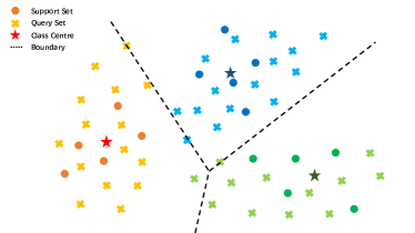
(a)

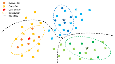
(b)

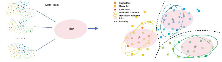
(c)

Figure 1: Illustrative Schematic of MetaQDA. (a) NCC classifier uses the class mean to induce linear decision boundaries. (b) QDA uses both the support class mean and covariance to induce a curved decision boundary, but easily overfits in a few-shot regime due. (c) MetaQDA meta-learns the QDA parameter prior to provide stable estimation of a non-linear decision boundary without overfitting.

Appendix B Additional Experimental Setting Details: Standard Few-shot Learning

Parameters for training the Conv-4 extractor  Following [61], we use stochastic gradient descent (SGD) with a multi-step learning rate schedule, momentum of 0.9, and the initial learning rate is set to 0.01 for both miniImageNet and CIFAR-FS, and 0.001 for tieredImageNet. At epochs 70 and 100 we reduce the learning rate by a factor of 0.1. Weight decay is set as 0.0001 through out training.

Parameters for training the ResNet-18 extractor  Following [61], we use stochastic gradient descent (SGD) with a multi-step learning rate schedule, momentum of 0.9, and the initial learning rate is set to 0.001 for tieredImageNet. At epochs 70 and 100 we reduce the learning rate by a factor of 0.1. Weight decay is set as 0.0001 throughout training. Batch size is 256 images.

Parameters for training the WRN-28-10 extractor  Following [37], as for 1-shot classification on miniImageNet, we use stochastic gradient descent (SGD) with a multi-step learning rate schedule, momentum of 0.9, and the initial learning rate is set to 0.001. For 5-shot classification on miniImageNetand 1-shot classification on tieredImageNet, we use ADAM optimiser. For CIFAR-FS, we use the pre-trained WRN backbone of S2M2.

Appendix C Additional Experimental Setting Details: Few-Shot Class Incremental Learning

Training setup  We follow the experimental setup of [56]. Specifically, we use the same 60 base classes to pre-train an initial ResNet-18 backbone using mini-batch size as 128 and use stochastic gradient descent (SGD) with the initial learning rate of 0.1, decreasing the learning rate to 0.01/0.001 after 30/40 epochs, respectively.

Meta-Training: The MetaQDA prior is then trained using Algorithm 1 (main manuscript) by generating episodes from the 60 base class set, using the feature extractor trained as above.

Meta-Testing: Due to our Bayesian class-conditional modeling, meta-testing decomposes over classes. Class-incremental learning is thus trivially realized by running MetaQDA’s update step for each new category, and adding the final mean and covariance to the set used by the final QDA classifier. We apply MetaQDA both for the many-shot base classes, and 5-shot incrementally added classes.

The results in Tab 6 of the main manuscript are averages generated by independently repeating both meta-train and meta-test (8 incremental sessions each) phases 10 times.

Appendix D Full Meta-Dataset Results

Implementation Details  We use the same backbone as SUR [7] and URT [34], and take the trained fused features by URT [34]. We use ADAM optimizer and cosine learning rate scheduler, and the initial learning rate is set to 0.0003, beta is set as 0.9 and 0.999. Weight decay is set as 0.0001 throughout training. The number of training episodes is 10000.

Results  Following [57], few-shot tasks are sampled with varing number of classes $N$, varying number of shots $K$ and class imbalance. Table 10 reports performance in accuracy over over 600 sampled meta-test tasks. Because most of the results have very similar confidence interval, we omit this part to make the table more readable. The results of other SotA algorithms are taken from URT [34] and SCNAP[1]. From the results we can see that MetaQDA performs well in both seen domains (left) and out-of-distribution unseen (right) domains. It achieves highest performance in 8 of 13 domains within the meta-dataset benchmark.

Model	ImageNet	Omniglot	Aircraft	Birds	DTD	Quickdraw	Fungi	Flower	Signs	Mscoco	MNIST	CIFAR10	CIFAR100
MAML [8]	32.4	71.9	52.8	47.2	56.7	50.5	21.0	70.9	34.2	24.1	NA	NA	NA
RelationNet [55]	30.9	86.6	69.7	54.1	56.6	61.8	32.6	76.1	37.5	27.4	NA	NA	NA
MatchingNet [59]	36.1	78.3	69.2	56.4	61.8	60.8	33.7	81.9	55.6	28.8	NA	NA	NA
Finetune [67]	43.1	71.1	72.0	59.8	69.1	47.1	38.2	85.3	66.7	35.2	NA	NA	NA
ProtoNet [52]	44.5	79.6	71.1	67.0	65.2	64.9	40.3	86.9	46.5	39.9	74.3	66.4	54.7
CNAP [48]	51.3	88.0	76.8	71.4	62.5	71.9	46.0	89.2	60.1	42.3	88.6	60.0	48.1
SCNAP [1]	58.6	91.7	82.4	74.9	67.8	77.7	46.9	90.7	73.5	46.2	93.9	74.3	60.5
SUR [7]	56.3	93.1	85.4	71.4	71.5	81.3	63.1	82.8	70.4	52.4	94.3	66.8	56.6
URT [34]	55.7	94.9	85.8	76.3	71.8	82.5	63.5	88.2	69.4	52.2	94.8	67.3	56.9
MetaQDA	56.5	96.3	86.5	75.1	73.4	82.6	63.7	87.4	73.8	49.8	94.3	68.2	57.8

Table 10: Full details of testing performance on the extended meta-dataset benchmark. Left is the in-domain (seen) dataset performance, where MetaQDA ranks first 5 times in 8 domains. Right is the out-of-domain (unseen) dataset performance, where MetaQDA ranks first 3 times in 5 domains. Overall, MetaQDA has state-of-the-art performance.

References

- [1] Peyman Bateni, Raghav Goyal, Vaden Masrani, Frank Wood, and Leonid Sigal. Improved few-shot visual classification. In CVPR, 2020.
- [2] Jonathan Baxter. A model of inductive bias learning. Journal of Artificial Intelligence Research, 12:149–198, 2000.
- [3] Luca Bertinetto, Joao F Henriques, Philip HS Torr, and Andrea Vedaldi. Meta-learning with differentiable closed-form solvers. In ICLR, 2019.
- [4] Wei-Yu Chen, Yen-Cheng Liu, Zsolt Kira, Yu-Chiang Wang, and Jia-Bin Huang. A closer look at few-shot classification. In ICLR, 2019.
- [5] M. Du, F. Yang, N. Zou, and X. Hu. Fairness in deep learning: A computational perspective. IEEE Intelligent Systems, 2020.
- [6] Nikita Dvornik, Cordelia Schmid, and Julien Mairal. Diversity with cooperation: Ensemble methods for few-shot classification. In ICCV, 2019.
- [7] Nikita Dvornik, Cordelia Schmid, and Julien Mairal. Selecting relevant features from a multi-domain representation for few-shot classification. In ECCV, 2020.
- [8] Chelsea Finn, Pieter Abbeel, and Sergey Levine. Model-agnostic meta-learning for fast adaptation of deep networks. In ICML, 2017.
- [9] Jerome Friedman, Trevor Hastie, and Robert Tibshirani. The elements of statistical learning, volume 1. Springer series in statistics New York, 2001.
- [10] Victor Garcia and Joan Bruna. Few-shot learning with graph neural networks. In ICLR, 2018.
- [11] Marta Garnelo, Dan Rosenbaum, Christopher Maddison, Tiago Ramalho, David Saxton, Murray Shanahan, Yee Whye Teh, Danilo Rezende, and S. M. Ali Eslami. Conditional neural processes. In ICML, 2018.
- [12] Andrew Gelman, John B. Carlin, Hal S. Stern, and Donald B. Rubin. Bayesian Data Analysis. Texts in statistical science. Chapman & Hall / CRC, 2nd edition, 2003.
- [13] Spyros Gidaris and Nikos Komodakis. Dynamic few-shot visual learning without forgetting. In CVPR, 2018.
- [14] Micah Goldblum, Steven Reich, Liam Fowl, Renkun Ni, Valeriia Cherepanova, and Tom Goldstein. Unraveling meta-learning: Understanding feature representations for few-shot tasks. In ICML, 2020.
- [15] Jonathan Gordon, John Bronskill, Matthias Bauer, Sebastian Nowozin, and Richard Turner. Meta-learning probabilistic inference for prediction. In ICLR, 2019.
- [16] Erin Grant, Chelsea Finn, Sergey Levine, Trevor Darrell, and Tom Griffiths. Recasting gradient-based meta-learning as hierarchical bayes. In ICLR, 2018.
- [17] Chuan Guo, Geoff Pleiss, Yu Sun, and Kilian Q Weinberger. On calibration of modern neural networks. In ICML, 2017.
- [18] Yunhui Guo, Noel C. F. Codella, Leonid Karlinsky, John R. Smith, Tajana Rosing, and Rogerio Feris. A broader study of cross-domain few-shot learning. In CVPR workshops, 2020.
- [19] Trevor Hastie, Robert Tibshirani, and Jerome Friedman. The Elements of Statistical Learning: Data Mining, Inference, and Prediction. Springer Science & Business Media, 2009.
- [20] Kaiming He, Xiangyu Zhang, Shaoqing Ren, and Jian Sun. Deep residual learning for image recognition. In CVPR, 2016.
- [21] Tom Heskes. Empirical bayes for learning to learn. In ICML, 2000.
- [22] Nathan Hilliard, Lawrence Phillips, Scott Howland, Artëm Yankov, Courtney D Corley, and Nathan O Hodas. Few-shot learning with metric-agnostic conditional embeddings. arXiv preprint arXiv:1802.04376, 2018.
- [23] Timothy Hospedales, Antreas Antoniou, Paul Micaelli, and Amos Storkey. Meta-learning in neural networks: A survey. arXiv preprint arXiv:2004.05439, 2020.
- [24] Andrey Ignatov, Radu Timofte, Andrei Kulik, Seungsoo Yang, Ke Wang, Felix Baum, Max Wu, Lirong Xu, and Luc Van Gool. Ai benchmark: All about deep learning on smartphones in 2019. arXiv preprint arXiv:1910.06663, 2019.
- [25] Xiang Jiang, Mohammad Havaei, Farshid Varno, Gabriel Chartrand, Nicolas Chapados, and Stan Matwin. Learning to learn with conditional class dependencies. In ICLR, 2019.
- [26] Jonathan Krause, Michael Stark, Jia Deng, and Li Fei-Fei. 3d object representations for fine-grained categorization. In ICCV workshops, 2013.
- [27] Alex Krizhevsky, Geoffrey Hinton, et al. Learning multiple layers of features from tiny images. Technical Report, 2009.
- [28] Lindsey Kuper, Guy Katz, Justin Gottschlich, Kyle Julian, Clark Barrett, and Mykel Kochenderfer. Toward Scalable Verification for Safety-Critical Deep Networks. In SysML, 2018.
- [29] Y Lecun and C Cortes. Mnist handwritten digit database. 2010.
- [30] Kwonjoon Lee, Subhransu Maji, Avinash Ravichandran, and Stefano Soatto. Meta-learning with differentiable convex optimization. In CVPR, 2019.
- [31] Aoxue Li, Tiange Luo, Tao Xiang, Weiran Huang, and Liwei Wang. Few-shot learning with global class representations. In ICCV, 2019.
- [32] Kai Li, Yulun Zhang, Kunpeng Li, and Yun Fu. Adversarial feature hallucination networks for few-shot learning. In CVPR, 2020.
- [33] Zhenguo Li, Fengwei Zhou, Fei Chen, and Hang Li. Meta-sgd: Learning to learn quickly for few-shot learning. arXiv preprint arXiv:1707.09835, 2017.
- [34] Lu Liu, William Hamilton, Guodong Long, Jing Jiang, and Hugo Larochelle. A universal representation transformer layer for few-shot image classification. In ICLR, 2021.
- [35] Yanbin Liu, Juho Lee, Minseop Park, Saehoon Kim, and Yi Yang. Transductive propagation network for few-shot learning. In ICLR, 2019.
- [36] D. J. C. MacKay. The evidence framework applied to classification networks. Neural Computation, 4(5):720–736, 1992.
- [37] Puneet Mangla, Nupur Kumari, Abhishek Sinha, Mayank Singh, Balaji Krishnamurthy, and Vineeth N Balasubramanian. Charting the right manifold: Manifold mixup for few-shot learning. In WACV, 2020.
- [38] Nikhil Mishra, Mostafa Rohaninejad, Xi Chen, and Pieter Abbeel. A simple neural attentive meta-learner. In ICLR, 2018.
- [39] Kevin P Murphy. Machine learning: a probabilistic perspective. MIT press, 2012.
- [40] Jeremy Nixon, Michael W Dusenberry, Linchuan Zhang, Ghassen Jerfel, and Dustin Tran. Measuring calibration in deep learning. In CVPR Workshops, 2019.
- [41] Boris Oreshkin, Pau Rodríguez López, and Alexandre Lacoste. Tadam: Task dependent adaptive metric for improved few-shot learning. In NeurIPS, 2018.
- [42] Massimiliano Patacchiola, Jack Turner, Elliot J Crowley, Michael O’Boyle, and Amos J Storkey. Bayesian meta-learning for the few-shot setting via deep kernels. In NeurIPS, 2020.
- [43] Siyuan Qiao, Chenxi Liu, Wei Shen, and Alan L Yuille. Few-shot image recognition by predicting parameters from activations. In CVPR, 2018.
- [44] Sachin Ravi and Hugo Larochelle. Optimization as a model for few-shot learning. In ICLR, 2017.
- [45] Sylvestre-Alvise Rebuffi, Alexander Kolesnikov, Georg Sperl, and Christoph H. Lampert. iCaRL: Incremental classifier and representation learning. In CVPR, 2017.
- [46] Mengye Ren, Renjie Liao, Ethan Fetaya, and Richard S. Zemel. Incremental few-shot learning with attention attractor networks. NeurIPS, 2019.
- [47] Mengye Ren, Eleni Triantafillou, Sachin Ravi, Jake Snell, Kevin Swersky, Joshua B Tenenbaum, Hugo Larochelle, and Richard S Zemel. Meta-learning for semi-supervised few-shot classification. In ICLR, 2018.
- [48] James Requeima, Jonathan Gordon, John Bronskill, Sebastian Nowozin, and Richard E Turner. Fast and flexible multi-task classification using conditional neural adaptive processes. In NIPS, 2019.
- [49] Olga Russakovsky, Jia Deng, Hao Su, Jonathan Krause, Sanjeev Satheesh, Sean Ma, Zhiheng Huang, Andrej Karpathy, Aditya Khosla, Michael Bernstein, et al. Imagenet large scale visual recognition challenge. IJCV, 115(3):211–252, 2015.
- [50] Andrei A Rusu, Dushyant Rao, Jakub Sygnowski, Oriol Vinyals, Razvan Pascanu, Simon Osindero, and Raia Hadsell. Meta-learning with latent embedding optimization. In ICLR, 2019.
- [51] Adam Santoro, David Raposo, David GT Barrett, Mateusz Malinowski, Razvan Pascanu, Peter Battaglia, and Timothy Lillicrap. A simple neural network module for relational reasoning. In NeurIPS, 2017.
- [52] Jake Snell, Kevin Swersky, and Richard S Zemel. Prototypical networks for few-shot learning. In NeurIPS, 2017.
- [53] Jiamei Sun, Sebastian Lapuschkin, Wojciech Samek, Yunqing Zhao, Ngai-Man Cheung, and Alexander Binder. Explanation-guided training for cross-domain few-shot classification. arXiv preprint arXiv:2007.08790, 2020.
- [54] Qianru Sun, Yaoyao Liu, Tat-Seng Chua, and Bernt Schiele. Meta-transfer learning for few-shot learning. In CVPR, 2019.
- [55] Flood Sung, Yongxin Yang, Li Zhang, Tao Xiang, Philip HS Torr, and Timothy M Hospedales. Learning to compare: Relation network for few-shot learning. In CVPR, 2018.
- [56] Xiaoyu Tao, Xiaopeng Hong, Xinyuan Chang, Songlin Dong, Xing Wei, and Yihong Gong. Few-shot class-incremental learning. In CVPR, 2020.
- [57] Eleni Triantafillou, Tyler Zhu, Vincent Dumoulin, Pascal Lamblin, Evci, et al. Meta-dataset: A dataset of datasets for learning to learn from few examples. In ICLR, 2019.
- [58] Hung-Yu Tseng, Hsin-Ying Lee, Jia-Bin Huang, and Ming-Hsuan Yang. Cross-domain few-shot classification via learned feature-wise transformation. In ICLR, 2020.
- [59] Oriol Vinyals, Charles Blundell, Tim Lillicrap, Daan Wierstra, et al. Matching networks for one shot learning. In NeurIPS, 2016.
- [60] Hongyu Wang, Henry Gouk, Eibe Frank, Bernhard Pfahringer, and Michael Mayo. A comparison of machine learning methods for cross-domain few-shot learning. In AJCAI, 2020.
- [61] Yan Wang, Wei-Lun Chao, Kilian Q Weinberger, and Laurens van der Maaten. Simpleshot: Revisiting nearest-neighbor classification for few-shot learning. arXiv preprint arXiv:1911.04623, 2019.
- [62] Yaqing Wang, Quanming Yao, James T. Kwok, and Lionel M. Ni. Generalizing from a few examples: A survey on few-shot learning. ACM Comput. Surv., 53(3), June 2020.
- [63] Chen Xing, Negar Rostamzadeh, Boris Oreshkin, and Pedro O O Pinheiro. Adaptive cross-modal few-shot learning. NeurIPS, 2019.
- [64] Mingzhang Yin, George Tucker, Mingyuan Zhou, Sergey Levine, and Chelsea Finn. Meta-learning without memorization. ICLR, 2020.
- [65] Jaesik Yoon, Taesup Kim, Ousmane Dia, Sungwoong Kim, Yoshua Bengio, and Sungjin Ahn. Bayesian model-agnostic meta-learning. In NeurIPS, 2018.
- [66] Sung Whan Yoon, Jun Seo, and Jaekyun Moon. Tapnet: Neural network augmented with task-adaptive projection for few-shot learning. In ICML, 2019.
- [67] Jason Yosinski, Jeff Clune, Yoshua Bengio, and Hod Lipson. How transferable are features in deep neural networks? In NeurIPS, 2014.
- [68] Xueting Zhang, Yuting Qiang, Sung Flood, Yongxin Yang, and Timothy M. Hospedales. RelationNet2: deep comparison columns for few-shot learning. In IJCNN, 2020.
- [69] Luisa M Zintgraf, Kyriacos Shiarlis, Vitaly Kurin, Katja Hofmann, and Shimon Whiteson. Fast context adaptation via meta-learning. In ICML, 2019.