A renormalizable left-right symmetric model with low scale seesaw mechanisms

Abstract

We propose a low scale renormalizable left-right symmetric theory that successfully explains the observed SM fermion mass hierarchy, the tiny values for the light active neutrino masses and is consistent with the lepton and baryon asymmetries of the Universe, the muon and electron anomalous magnetic moments as well as the with the constraints arising from the meson oscillations. In the proposed model the top and exotic quarks obtain masses at tree level, whereas the masses of the bottom, charm and strange quarks, tau and muon leptons are generated from a tree level Universal Seesaw mechanism, thanks to their mixings with the charged exotic vector like fermions. The masses for the first generation SM charged fermions arise from a radiative seesaw mechanism at one loop level, mediated by charged vector like fermions and electrically neutral scalars. The light active neutrino masses are produced from a one-loop level inverse seesaw mechanism mediated by electrically neutral scalar singlets and right handed Majorana neutrinos. Our model is also consistent with the experimental constraints arising from the Higgs diphoton decay rate as well as with the constraints arising from charged lepton flavor violation. We also discuss the $Z^{\prime}$ and heavy scalar production at a proton-proton collider.

DOI:10.1016/j.nuclphysb.2022.115696

I Introduction

Despite the great success of the Standard Model (SM) as a theory of fundamental interactions, it features drawbacks such as, for example, the lack of explanation of the SM flavor structure; in particular, the observed pattern of SM fermion masses and mixings, the origin of Dark Matter (DM), the source of parity violation in electroweak (EW) interactions, the lepton and baryon asymmetries of the Universe and the anomalous magnetic moments of the muon and electron. In order to address these issues, it is necessary to propose a possible more general higher energy theory. In this sense, left-right symmetric electroweak extensions of the Weinberg-Salam theory have many appealing features, foremost of which is to address the origin of parity violation as a low energy effect, a remanent of its breaking at a certain high energy scale. We are therefore proposing, as a possible explanation of the problems listed before, a minimal renormalizable Left-right symmetric theory  Pati:1974yy ; Mohapatra:1974gc based on the gauge symmetry $SU(3)_{C}\times SU\left(2\right)_{L}\times SU\left(2\right)_{R}\times U\left(1\right)_{B-L}$, supplemented by the $Z_{4}^{\left(1\right)}\times Z_{4}^{\left(2\right)}$ discrete group, where the $Z_{4}^{\left(1\right)}$ symmetry is completely broken, whereas the $Z_{4}^{\left(2\right)}$ symmetry is broken down to the preserved $Z_{2}$, thus allowing the implementation of a radiative inverse seesaw mechanism to generate the tiny masses of the light active neutrinos. In the proposed model, the top and exotic quarks obtain masses at tree level from the Yukawa interactions, whereas the masses of the bottom, charm and strange quarks, tau and muon leptons arise from a tree level Universal Seesaw mechanism Davidson:1987mh ; Davidson:1987mi . The masses for the first generation SM charged fermions are generated from a one loop level radiative seesaw mechanism mediated by charged vector like fermions and electrically neutral scalars. Unlike Davidson:1987mh , where the tree level Universal Seesaw mechanism was first implemented to generate the masses of all SM charged fermions and light active neutrinos, in our model we use the tree level Universal Seesaw mechanism only for the charm, bottom, strange quarks, tau and muon leptons. Furthermore, whereas in the model of Davidson:1987mh the light active neutrino masses are generated from a type I seesaw mechanism, in our model we implement the one loop level inverse seesaw mechanism mediated by electrically neutral scalar singlets and right handed Majorana neutrinos, in order to produce the tiny masses of the light active neutrinos. Some recent left-right symmetric models have been considered in Refs. CarcamoHernandez:2018hst ; Dekens:2014ina ; Nomura:2016run ; Brdar:2018sbk ; Ma:2020lnm ; Babu:2020bgz . Unlike the model of Ref CarcamoHernandez:2018hst , where non renormalizable Yukawa interactions are employed for the implementation of a Froggatt Nielsen mechanism to produce the current SM fermion mass and mixing pattern, our proposed model is a fully renormalizable theory, with minimal particle content and symmetries, where tree level Universal as well as one-loop level radiative seesaw and inverse seesaw mechanisms are combined to explain the observed hierarchy of SM fermion masses and fermionic mixing parameters. Furthermore, unlike Ref. CarcamoHernandez:2018hst our model successfully explains the electron and muon anomalous magnetic moments and includes a discussion about leptogenesis and collider signatures of heavy scalar and $Z^{\prime}$ gauge bosons, which is not presented in CarcamoHernandez:2018hst .

In our current model, the charged vector-like leptons responsible for the tree level Universal and one-loop level radiative seesaw mechanism that produces the SM charged fermion mass hierarchy, allows to reproduce the measured values of the muon and electron anomalous magnetic moments, thus linking the fermion mass generation mechanism and the $g-2$ anomalies, which is not given in the left-right symmetric model of Ref. CarcamoHernandez:2018hst . Moreover, unlike the left-right symmetric theory of Ref. Ma:2020lnm , our model does not rely on the inclusion of scalar leptoquarks to generate one loop level masses for the SM charged fermions and light active neutrinos. Besides that, whereas in the left-right symmetric model of Babu:2020bgz the light active neutrino masses are generated from a combination of type I and type II seesaw mechanisms, in our model the tiny masses of the light active neutrinos are produced from an inverse seesaw mechanism at one loop level. Another difference of our model with the one proposed of Babu:2020bgz is that in the former a mechanism for explaining the SM charged fermion mass hierarchy is presented, whereas in the latter such mechanism is not given. Furthermore, whereas in the models of Refs. Brdar:2018sbk and Nomura:2016run , the masses of the light active neutrinos are generated from a tree level inverse and radiative type I sessaw mechanisms, respectively, in our model we use the inverse seesaw mechanism at one loop level to produce the tiny masses of the light active neutrinos. In addition, our model includes a dynamical mechanism to generate the SM charged fermion mass pattern, which is not presented in the model of Ref. Brdar:2018sbk .

On the other hand, the renormalizable left-right symmetric theory proposed in this paper has similar amount of particle content compared to the left-right symmetric model considered in Dekens:2014ina . For instance, whereas the scalar sector of left-right symmetric model of Ref. Dekens:2014ina has one scalar bidoublet (having 8 degrees of freedom), one $SU(2)_{L}$ scalar triplet (transforming as a $SU(2)_{R}$ singlet) (having 6 degrees of freedom) and one $SU(2)_{R}$ scalar triplet (transforming as a $SU(2)_{L}$ singlet) (having 6 degrees of freedom), thus amounting to 14 physical scalar degrees of freedom (after substracting the number of Goldstone bosons), our current left-right model has one scalar bidoublet (8 degrees of freedom), two $SU(2)_{L}$ scalar doublets (8 degrees of freedom), two $SU(2)_{R}$ scalar doublets (8 degrees of freedom), two electrically neutral gauge singlet real scalars (2 degrees of freedom) and two electrically neutral gauge singlet complex scalars (4 degrees of freedom), which corresponds to 24 physical scalar degrees of freedom. Despite our model has more scalar degrees of freedom than the one proposed in Dekens:2014ina , the advantage of our proposal with respect to the ones presented in Dekens:2014ina ; Brdar:2018sbk is that in the former a mechanism that naturally explains the SM fermion mass hierarchy is presented, whereas the latter does not include such mechanism.

The paper is organized as follows. In section II we outline the proposed model. The implications of our model in the SM fermion hierarchy is discussed in section III. The implications of our model in charged lepton flavor violation are described in section IV. The consequences of our model in leptogenesis are described in section V, while the model scalar potential is analyzed in section VI. The implications of our model in the Higgs diphoton decay are discussed in section VII, and in section VIII we analyze its application to the muon and electron anomalous magnetic moments. The $Z^{\prime}$ and heavy scalar production at a proton-proton collider are discussed in sections IX and X, respectively. The implications of our model in meson oscillations are discussed in section XI. We conclude in section XII. An analytical argument of the minimal number of fermionic seesaw mediators required to generate the masses of SM fermions via a seesaw-like mechanism is presented in Appendix A.

II An extended Left-Right symmetric model

Before providing a detailed explanation of our left-right symmetric model, we will explain the reasoning behind introducing extra scalars, fermions and symmetries, needed for implementing an interplay of tree level universal and radiative seesaw mechanism to explain the SM charged fermion mass hierarchy and one loop level inverse seesaw mechanism to generate the tiny neutrino masses. It is worth mentioning that in our proposed model, the mass of the top quark will be generated from a renormalizable Yukawa operator, with an order one Yukawa coupling, i.e.

$$\overline{Q}_{3L}\Phi Q_{iR},\hskip 42.67912pti=1,2,3$$ (1)

where $Q_{3L}$ and $Q_{iR}$ are $SU\left(2\right)_{L}$ and $SU\left(2\right)_{R}$ quark doublets, respectively:

$$Q_{iL}=\left(\begin{array}[]{c}u_{iL}\\ d_{iL}\end{array}\right),\hskip 42.67912ptQ_{iR}=\left(\begin{array}[]{c}\overline{u}_{iR}\\ \overline{d}_{iR}\end{array}\right),\hskip 42.67912pti=1,2,3,$$ (2)

whereas $\Phi$ is a scalar bidoblet, with the VEV pattern

$$\left\langle\Phi\right\rangle=\left(\begin{array}[]{cc}v_{1}&0\\ 0&v_{2}\end{array}\right),$$ (3)

where we have set $v_{2}=0$ to prevent a bottom quark mass arising from the above given Yukawa interaction. Now, to generate tree level masses via a Universal Seesaw mechanism for the bottom, strange and charm quarks, as well as for the tau and muon leptons, one loop level masses for the first generation SM charged fermions and the tiny masses for the light active neutrinos via a one loop level inverse seesaw mechanism, we need to forbid the operators:

$$\overline{Q}_{nL}\Phi Q_{iR},\hskip 42.67912pt\overline{Q}_{nL}\widetilde{\Phi}Q_{iR},\hskip 42.67912ptn=1,2,\hskip 42.67912pti=1,2,3,$$

$$\overline{L}_{iL}\widetilde{\Phi}L_{jR},\hskip 42.67912pt\overline{L}_{iL}\widetilde{\chi}_{L}N_{jR},\hskip 42.67912pt\left(m_{N}\right)_{ij}\overline{N}_{iR}N_{jR}^{C},\hskip 42.67912pti,j=1,2,3.$$ (4)

where $\chi_{L}$ ($\chi_{R}$) is a $SU\left(2\right)_{L}$ ($SU\left(2\right)_{R}$) scalar doublet. Furthermore, $L_{iL}$ and $L_{iR}$ are $SU\left(2\right)_{L}$ and $SU\left(2\right)_{R}$ lepton doublets, respectively:

$$L_{iL}=\left(\begin{array}[]{c}\nu_{iL}\\ e_{iL}\end{array}\right),\hskip 42.67912ptL_{iR}=\left(\begin{array}[]{c}\nu_{iR}\\ e_{iR}\end{array}\right),\hskip 42.67912pti=1,2,3,$$ (5)

while $N_{iR}$ ($i=1,2,3$) are gauge singlet neutral leptons. As it will be shown in the following, the aforementioned gauge singlet neutral leptons are necessary for the implementation of the one loop level inverse seesaw mechanism that produces the tiny masses of the light active neutrinos.

Furthermore, the successfull implentation of the tree level universal and radiative seesaw mechanism to explain the SM charged fermion mass hierarchy and of the one loop level inverse seesaw mechanism to generate the tiny neutrino masses, requires the following operators:

$$\overline{Q}_{3L}\chi_{L}B_{1R},\hskip 42.67912pt\overline{Q}_{nL}\chi_{L}B_{2R},\hskip 42.67912pt\overline{B}_{nL}\chi_{R}^{\dagger}Q_{iR},\hskip 42.67912pt\overline{B}_{1L}\rho B_{1R},\hskip 42.67912pt\overline{B}_{2L}\sigma B_{2R},$$

$$\overline{Q}_{nL}\widetilde{\chi}_{L}T_{R},\hskip 42.67912pt\overline{T}_{L}\widetilde{\chi}_{R}^{\dagger}Q_{iR},\hskip 42.67912pt\overline{T}_{L}\sigma T_{R},\hskip 42.67912ptn=1,2,\hskip 42.67912pti=1,2,3,$$

$$\overline{Q}_{nL}\phi_{L}B_{R}^{\prime},\hskip 28.45274pt\bar{B}_{L}^{\prime}\phi_{R}^{\dagger}Q_{iR},\hskip 28.45274pt\overline{Q}_{nL}\widetilde{\phi}_{L}T_{R}^{\prime},\hskip 28.45274pt\bar{T}_{L}^{\prime}\widetilde{\phi}_{R}^{\dagger}Q_{iR},\hskip 28.45274pt\bar{B}_{L}^{\prime}\sigma B_{R}^{\prime},\hskip 28.45274pt\bar{T}_{L}^{\prime}\sigma T_{R}^{\prime},$$

$$\overline{L}_{iL}\chi_{L}E_{nR},\hskip 28.45274pt\overline{E}_{nL}\chi_{R}^{\dagger}L_{jR},\hskip 28.45274pt\overline{L}_{iL}\phi_{L}E_{R}^{\prime},\hskip 28.45274pt\bar{E}_{L}^{\prime}\phi_{R}^{\dagger}L_{iR},\hskip 28.45274pt\overline{E}_{nL}\rho E_{nR},\hskip 28.45274pt\bar{E}_{L}^{\prime}\rho E_{R}^{\prime},$$

$$\overline{L}_{iL}\Phi L_{jR},\hskip 28.45274pt\overline{N_{iR}^{C}}\widetilde{\chi}_{R}^{\dagger}L_{jR},\hskip 28.45274pt\overline{\Omega}_{nR}\Omega_{nR}^{C}\eta,\hskip 28.45274pt\overline{N}_{nR}\Omega_{kR}^{C}\varphi,\hskip 28.45274ptn,k=1,2.$$ (6)

This requires to add $Z_{4}^{\left(1\right)}$ and $Z_{4}^{\left(2\right)}$ discrete symmetries, which are spontaneously broken, where the former is completely broken, and the latter is broken down to the preserved $Z_{2}$ symmetry. Such remaining conserved $Z_{2}$ symmetry allows to implement an inverse seesaw mechanism at one loop level to produce the tiny neutrino masses. Let us note that the gauge singlet neutral leptons $\Omega_{nR}$ ($n=1,2$) are crucial for generating the term $\left(m_{N}\right)_{ij}\overline{N}_{iR}N_{jR}^{C}$ ($i,j=1,2,3$) at one loop level, thus allowing the implementation of the one-loop level inverse seesaw mechanism. Additionally, the above mentioned exotic neutral lepton content is the minimal one required to generate the masses for two light active neutrinos, as required from the neutrino oscillation experimental data. Besides that, the SM charged fermion sector has to be extended to include the following heavy fermions: up type quarks $T$, $T^{\prime}$, down type quarks $B_{n}$, $B^{\prime}$ and charged leptons $E_{n}$ ($n=1,2$), $E^{\prime}$ in singlet representations under $SU\left(2\right)_{L}\times SU\left(2\right)_{R}$. As a consequence of the above mentioned exotic charged fermion spectrum, the rows and columns of the tree level SM charged fermion mass matrices will be linearly dependent, thus implying that the first generation SM charged fermions will be massless at tree level. The one loop level corrections to these matrices mediated by the $T^{\prime}$, $B^{\prime}$ and $E^{\prime}$ fermionic fields will make thus rows and columns linearly indenpendent, thus yielding one-loop level masses for the up and down quarks as well as for the electron. Consequently, the aforementioned exotic charged fermion spectrum is the minimal necessary so that no massless charged SM-fermions would appear in the model, provided that one loop level corrections are taken into account. For a more detailed explanation of the analytical argument of the minimal number of fermionic seesaw mediators required to generate the masses of SM fermions via a seesaw-like mechanism the reader is referred to Appendix A.

On the other hand, in what regards the scalar sector, it is worth mentioning that $\chi_{L}$, $\phi_{L}$ and $\chi_{R}$, $\phi_{R}$ are $SU\left(2\right)_{L}$ and $SU\left(2\right)_{R}$ scalar doublets, respectively, whereas $\eta$, $\sigma$, $\rho$ and $\varphi$ are gauge singlet scalars. Furthermore, the $\chi_{L}$ ($\chi_{R}$) scalar is crucial for generating mass mixing terms between left (right) handed SM charged fermions and right (left) handed exotic charged fermions. Furthermore, the $SU\left(2\right)_{R}$ scalar doublet $\chi_{R}$ is crucial for triggering the spontaneous breaking of the $SU\left(2\right)_{L}\times SU\left(2\right)_{R}\times U\left(1\right)_{B-L}$ symmetry down to the SM electroweak gauge group. Besides that, the $\sigma$ and $\rho$ are gauge singlet scalars, whose inclusion is necessary for generating the masses of the charged exotic fermions. On the other hand, the gauge singlet scalars $\eta$ and $\varphi$ are required to generate tree and one loop level masses for the Majorana neutrinos $\Omega_{nR}$ ($n=1,2$) and $N_{iR}$ ($i=1,2,3$), which is crucial for a radiative generation of the $\mu$ parameter of the inverse seesaw mechanism. Moreover, the inclusion of the scalar bidoublet $\Phi$ is crucial to generate a tree level top quark mass, as well as the Dirac neutrino submatrix, as will be shown below. The aforementioned scalar content is the minimal required for a successful implementation of the tree level universal and one loop level radiative seesaw mechanisms to explain the SM charged fermion mass hierarchy, as well as of the one loop level inverse seesaw mechanism to produce the tiny neutrino masses. By suitable charge assignments to be specified below, we can implement the aforementioned seesaw mechanisms, useful for explaining the SM fermion mass hierarchy.

Our proposed model is based on the gauge symmetry $SU(3)_{C}\times SU\left(2\right)_{L}\times SU\left(2\right)_{R}\times U\left(1\right)_{B-L}$, supplemented by the $Z_{4}^{\left(1\right)}\times Z_{4}^{\left(2\right)}$ discrete group, where the full symmetry $\mathcal{G}$ exhibites the following breaking scheme:

$$\mathcal{G}=SU(3)_{C}\times SU\left(2\right)_{L}\times SU\left(2\right)_{R}\times U\left(1\right)_{B-L}\times Z_{4}^{\left(1\right)}\times Z_{4}^{\left(2\right)}$$

$$\hskip 99.58464pt\Downarrow v_{\sigma},v_{\eta},v_{\rho}$$

$$\hskip 42.67912ptSU(3)_{C}\times SU\left(2\right)_{L}\times SU\left(2\right)_{R}\times U\left(1\right)_{B-L}$$

$$\hskip 99.58464pt\Downarrow v_{R}$$

$$\hskip 42.67912ptSU(3)_{C}\times SU\left(2\right)_{L}\times U\left(1\right)_{Y}\times Z_{2}$$

$$\hskip 99.58464pt\Downarrow v_{1},v_{L}$$

$$\hskip 42.67912ptSU(3)_{C}\otimes U\left(1\right)_{Q}\times Z_{2}$$ (7)

Both $Z_{4}^{\left(1\right)}$ and $Z_{4}^{\left(2\right)}$ discrete groups are spontaneously broken, and are crucial for avoiding a tree level inverse seesaw mechanism. The $Z_{4}^{\left(1\right)}$ symmetry is completely broken, whereas the $Z_{4}^{\left(2\right)}$ symmetry is broken down to the preserved $Z_{2}$ symmetry. It is assumed that such discrete symmetries are broken at the scale much larger than the scale of breaking of the left-right symmetry. We further assume that the left-right symmetry breaking scale is about $v_{R}\sim\mathcal{O}(10)$ TeV. In addition, the $Z_{4}^{\left(2\right)}$ symmetry, which is spontaneously broken to the preserved $Z_{2}$, is crucial in order to forbid the appearance of the term $\left(m_{N}\right)_{ij}\overline{N}_{iR}N_{jR}^{C}$ at tree level, thus allowing the implementation of the one loop level inverse seesaw mechanism that generates the light active neutrino masses. Besides that, the spontaneously broken $Z_{4}^{\left(1\right)}$ symmetry is crucial to prevent tree level Yukawa mass terms involving the scalar bidoublet and SM charged fermions lighter than the top quark. As we will see in the following, in the SM fermion sector only the top quark will acquire its mass from a renormalizable Yukawa interaction with the scalar bidoublet, whereas the SM charged fermions lighter than the top quark will get their masses from tree level Universal seesaw and radiative seesaw mechanisms.

The fermion assignments under the $SU(3)_{C}\times SU\left(2\right)_{L}\times SU\left(2\right)_{R}\times U\left(1\right)_{B-L}$ group are:

$$Q_{iL} = \left(\begin{array}[]{c}u_{iL}\\ d_{iL}\end{array}\right)\sim\left(\mathbf{3},\mathbf{2,1},\frac{1}{3}\right),\hskip 42.67912ptQ_{iR}=\left(\begin{array}[]{c}\overline{u}_{iR}\\ \overline{d}_{iR}\end{array}\right)\sim\left(\mathbf{3},\mathbf{1,2},\frac{1}{3}\right),\hskip 42.67912pti=1,2,3,$$ (12)

$$L_{iL} = \left(\begin{array}[]{c}\nu_{iL}\\ e_{iL}\end{array}\right)\sim\left(\mathbf{1},\mathbf{2,1},-1\right),\hskip 42.67912ptL_{iR}=\left(\begin{array}[]{c}\nu_{iR}\\ e_{iR}\end{array}\right)\sim\left(\mathbf{1},\mathbf{1,2},-1\right),\hskip 42.67912pti=1,2,3,$$ (17)

$$T_{R} \sim \left(\mathbf{3},\mathbf{1,1},\frac{4}{3}\right),\hskip 42.67912ptT_{L}\sim\left(\mathbf{3},\mathbf{1,1},\frac{4}{3}\right),\hskip 42.67912ptT_{R}^{\prime}\sim\left(\mathbf{3},\mathbf{1,1},\frac{4}{3}\right),\hskip 42.67912ptT_{L}^{\prime}\sim\left(\mathbf{3},\mathbf{1,1},\frac{4}{3}\right),$$

$$B_{nR} \sim \left(\mathbf{3},\mathbf{1,1},-\frac{2}{3}\right),\hskip 42.67912ptB_{nL}\sim\left(\mathbf{3},\mathbf{1,1},-\frac{2}{3}\right),\hskip 42.67912ptB_{R}^{\prime}\sim\left(\mathbf{3},\mathbf{1,1},-\frac{2}{3}\right),\hskip 42.67912ptB_{L}^{\prime}\sim\left(\mathbf{3},\mathbf{1,1},-\frac{2}{3}\right),$$

$$E_{nR} \sim \left(\mathbf{1},\mathbf{1,1},-2\right),\hskip 42.67912ptE_{nL}\sim\left(\mathbf{1},\mathbf{1,1},-2\right),\hskip 42.67912ptE_{R}^{\prime}\sim\left(\mathbf{1},\mathbf{1,1},-2\right),\hskip 42.67912ptE_{L}^{\prime}\sim\left(\mathbf{1},\mathbf{1,1},-2\right),$$

$$N_{iR} \sim \left(\mathbf{1},\mathbf{1,1},0\right),\hskip 42.67912pt\Omega_{nR}\sim\left(\mathbf{1},\mathbf{1,1},0\right),\hskip 42.67912ptn=1,2.$$ (18)

Let us note that we have extended the fermion sector of the original left-right symmetric model model by introducing two exotic up type quarks $T$, $T^{\prime}$, three exotic down type quarks $B_{n}$ ($n=1,2$), $B^{\prime}$, three charged leptons $E_{n}$, $E^{\prime}$ and five Majorana neutrinos, i.e., $N_{iR}$ ($i=1,2,3$) and $\Omega_{nR}$ ($n=1,2$). Such exotic fermions are assigned as singlet representations of the $SU\left(2\right)_{L}\times SU\left(2\right)_{R}$ group. The above mentioned exotic fermion content is the minimal one required to generate tree level masses via a Universal seesaw mechanism for the bottom, charm and strange quarks, as well as the tau and muon, and one loop level masses for the first generation SM charged fermions, i.e., the up, down quarks, and the electron.

The scalar assignments under the $SU(3)_{C}\times SU\left(2\right)_{L}\times SU\left(2\right)_{R}\times U\left(1\right)_{B-L}$ group are:

$$\Phi = \left(\begin{array}[]{cc}\frac{1}{\sqrt{2}}\left(v_{1}+\phi_{1R}^{0}+i\phi_{1I}^{0}\right)&\phi_{2}^{+}\\ \phi_{1}^{-}&\frac{1}{\sqrt{2}}\left(v_{2}+\phi_{2R}^{0}+i\phi_{2I}^{0}\right)\end{array}\right)\sim\left(\mathbf{1},\mathbf{2,2},0\right),$$ (21)

$$\chi_{L} = \left(\begin{array}[]{c}\chi_{L}^{+}\\ \frac{1}{\sqrt{2}}\left(v_{L}+\mathop{\mathrm{R}e}\chi_{L}^{0}+i\mathop{\mathrm{I}m}\chi_{L}^{0}\right)\end{array}\right)\sim\left(\mathbf{1},\mathbf{2,1},1\right),\hskip 28.45274pt\chi_{R}=\left(\begin{array}[]{c}\chi_{R}^{+}\\ \frac{1}{\sqrt{2}}\left(v_{R}+\mathop{\mathrm{R}e}\chi_{R}^{0}+i\mathop{\mathrm{I}m}\chi_{R}^{0}\right)\end{array}\right)\sim\left(\mathbf{1},\mathbf{1,2},1\right),$$ (26)

$$\phi_{L} = \left(\begin{array}[]{c}\phi_{L}^{+}\\ \frac{1}{\sqrt{2}}\left(\mathop{\mathrm{R}e}\phi_{L}^{0}+i\mathop{\mathrm{I}m}\phi_{L}^{0}\right)\end{array}\right)\sim\left(\mathbf{1},\mathbf{2,1},1\right),\hskip 28.45274pt\phi_{R}=\left(\begin{array}[]{c}\phi_{R}^{+}\\ \frac{1}{\sqrt{2}}\left(\mathop{\mathrm{R}e}\phi_{R}^{0}+i\mathop{\mathrm{I}m}\phi_{R}^{0}\right)\end{array}\right)\sim\left(\mathbf{1},\mathbf{1,2},1\right),$$ (31)

$$\sigma \sim \left(\mathbf{1},\mathbf{1,1},0\right),\hskip 28.45274pt\varphi\sim\left(\mathbf{1},\mathbf{1,1},0\right),\hskip 28.45274pt\eta\sim\left(\mathbf{1},\mathbf{1,1},0\right),\hskip 28.45274pt\rho\sim\left(\mathbf{1},\mathbf{1,1},0\right).$$ (32)

To implement the tree level Universal mechanism we have introduced the scalars $\chi_{L}$, $\chi_{R}$ which are responsible for generating tree level mixings between the exotic and SM fermions. Besides that, the scalar fields $\phi_{L}$, $\phi_{R}$ are required for the implementation of the radiative seesaw mechanism that produces the masses for the first generation SM charged fermions.

We have further introduced the gauge singlet scalars $\eta$ and $\varphi$ which are crucial for the implementation of the radiative inverse seesaw mechanism necessary to produce the light active neutrino masses. Furthermore, the gauge singlet scalar $\sigma$ provides tree level masses for the exotic $T$ , $T^{\prime}$, $B_{2}$ and $B^{\prime}$ quarks. Besides that, the gauge singlet scalars $\rho$ and $\eta$ are included in the scalar spectrum in order to provide tree level masses for the exotic down type quark $B_{1}$, for the exotic leptons $E_{n}$, $E^{\prime}$ and $\Omega_{nR}$ ($n=1,2$), without the need of invoking soft-breaking mass terms. Furthermore, we have also included the scalar bidoublet $\Phi$, which is responsible for generating the top quark mass from the renormalizable Yukawa operator $\overline{Q}_{3L}\Phi Q_{iR}$ ($i=1,2,3$).

The vacuum expectation values (VEVs) of the scalars $\Phi$, $\chi_{L}$ and $\chi_{R}$ are:

$$\left\langle\Phi\right\rangle=\left(\begin{array}[]{cc}v_{1}&0\\ 0&v_{2}\end{array}\right),\hskip 42.67912pt\left\langle\chi_{L}\right\rangle=\left(\begin{array}[]{c}0\\ v_{L}\end{array}\right),\hskip 42.67912pt\left\langle\chi_{R}\right\rangle=\left(\begin{array}[]{c}0\\ v_{R}\end{array}\right),$$ (33)

where for the sake of simplicity we will set $v_{2}=0$.

The fermion assignments under $Z_{4}^{\left(1\right)}\times Z_{4}^{\left(2\right)}$ are:

$$Q_{nL} \sim \left(-1,-1\right),\hskip 28.45274ptQ_{3L}\sim\left(i,-1\right),\hskip 28.45274ptQ_{jR}\sim\left(1,1\right),\hskip 28.45274pt$$

$$T_{L} \sim \left(1,1\right),\hskip 28.45274ptT_{R}\sim\left(1,-1\right),\hskip 28.45274ptT_{L}^{\prime}\sim\left(1,-i\right),\hskip 28.45274ptT_{R}^{\prime}\sim\left(1,i\right),$$

$$B_{nL} \sim \left(1,1\right),\hskip 28.45274ptB_{1R}\sim\left(-i,-1\right),\hskip 28.45274ptB_{2R}\sim\left(1,-1\right),\hskip 28.45274ptB_{L}^{\prime}\sim\left(1,i\right),\hskip 28.45274ptB_{R}^{\prime}\sim\left(1,-i\right),$$

$$L_{jL} \sim \left(1,i\right),\hskip 28.45274ptL_{jR}\sim\left(-i,-i\right),\hskip 28.45274ptN_{jR}\sim\left(i,i\right),\hskip 28.45274pt\Omega_{nR}\sim\left(-i,1\right),\hskip 28.45274ptj=1,2,3,$$

$$E_{nL} \sim \left(-i,-i\right),\hskip 28.45274ptE_{nR}\sim\left(-1,i\right),\hskip 28.45274ptE_{L}^{\prime}\sim\left(-i,1\right),\hskip 28.45274ptE_{R}^{\prime}\sim\left(-1,-1\right),\hskip 28.45274ptn=1,2.$$

The scalar fields have the following $Z_{4}^{\left(1\right)}\times Z_{4}^{\left(2\right)}$ assignments:

$$\Phi \sim \left(i,-1\right),\hskip 28.45274pt\chi_{L}\sim\left(-1,1\right),\hskip 28.45274pt\chi_{R}\sim\left(1,1\right),\hskip 28.45274pt\phi_{L}\sim\left(-1,-i\right),\hskip 28.45274pt\phi_{R}\sim\left(1,-i\right)$$

$$\varphi \sim \left(1,i\right),\hskip 28.45274pt\sigma\sim\left(1,-1\right),\hskip 28.45274pt\eta\sim\left(-1,1\right),\hskip 28.45274pt\rho\sim\left(i,-1\right).$$ (34)

The fermion and scalar assignments under the $SU(3)_{C}\times SU(2)_{L}\times SU(2)_{R}\times U(1)_{B-L}\times Z_{4}^{\left(1\right)}\times Z_{4}^{\left(2\right)}$ symmetry are shown in Tables 1 and 2, respectively.

$$\begin{array}[]{|c|c|c|c|c|c|c|c|c|c|c|c|c|c|c|c|c|c|c|c|c|}\hline\cr&Q_{nL}&Q_{3L}&Q_{iR}&L_{iL}&L_{iR}&T_{L}&T_{R}&T_{L}^{\prime}&T_{R}^{\prime}&B_{nL}&B_{1R}&B_{2R}&B_{L}^{\prime}&B_{R}^{\prime}&E_{nL}&E_{nR}&E_{L}^{\prime}&E_{R}^{\prime}&N_{iR}&\Omega_{nR}\\ \hline\cr SU(3)_{C}&\mathbf{3}&\mathbf{3}&\mathbf{3}&\mathbf{1}&\mathbf{1}&\mathbf{3}&\mathbf{3}&\mathbf{3}&\mathbf{3}&\mathbf{3}&\mathbf{3}&\mathbf{3}&\mathbf{3}&\mathbf{3}&\mathbf{1}&\mathbf{1}&\mathbf{1}&\mathbf{1}&\mathbf{1}&\mathbf{1}\\ \hline\cr SU\left(2\right)_{L}&\mathbf{2}&\mathbf{2}&\mathbf{1}&\mathbf{2}&\mathbf{1}&\mathbf{1}&\mathbf{1}&\mathbf{1}&\mathbf{1}&\mathbf{1}&\mathbf{1}&\mathbf{1}&\mathbf{1}&\mathbf{1}&\mathbf{1}&\mathbf{1}&\mathbf{1}&\mathbf{1}&\mathbf{1}&\mathbf{1}\\ \hline\cr SU\left(2\right)_{R}&\mathbf{1}&\mathbf{1}&\mathbf{2}&\mathbf{1}&\mathbf{2}&\mathbf{1}&\mathbf{1}&\mathbf{1}&\mathbf{1}&\mathbf{1}&\mathbf{1}&\mathbf{1}&\mathbf{1}&\mathbf{1}&\mathbf{1}&\mathbf{1}&\mathbf{1}&\mathbf{1}&\mathbf{1}&\mathbf{1}\\ \hline\cr U\left(1\right)_{B-L}&\frac{1}{3}&\frac{1}{3}&\frac{1}{3}&-1&-1&\frac{4}{3}&\frac{4}{3}&\frac{4}{3}&\frac{4}{3}&-\frac{2}{3}&-\frac{2}{3}&-\frac{2}{3}&-\frac{2}{3}&-\frac{2}{3}&-2&-2&-2&-2&0&0\\ \hline\cr Z_{4}^{\left(1\right)}&-1&i&1&1&-i&1&1&1&1&1&-i&1&1&1&-i&-1&-i&-1&i&-i\\ \hline\cr Z_{4}^{\left(2\right)}&-1&-1&1&i&-i&1&-1&-i&i&1&-1&-1&i&-i&-i&i&1&-1&i&1\\ \hline\cr\end{array}$$

Table 1: Fermion assignments under $SU(3)_{C}\times SU(2)_{L}\times SU(2)_{R}\times U(1)_{B-L}\times Z_{4}^{\left(1\right)}\times Z_{4}^{\left(2\right)}$. Here $i=1,2,3$ and $n=1,2$

$$\begin{array}[]{|c|c|c|c|c|c|c|c|c|c|}\hline\cr&\Phi&\chi_{L}&\chi_{R}&\phi_{L}&\phi_{R}&\varphi&\sigma&\eta&\rho\\ \hline\cr SU(3)_{C}&\mathbf{1}&\mathbf{1}&\mathbf{1}&\mathbf{1}&\mathbf{1}&\mathbf{1}&\mathbf{1}&\mathbf{1}&\mathbf{1}\\ \hline\cr SU\left(2\right)_{L}&\mathbf{2}&\mathbf{2}&\mathbf{1}&\mathbf{2}&\mathbf{1}&\mathbf{1}&\mathbf{1}&\mathbf{1}&\mathbf{1}\\ \hline\cr SU\left(2\right)_{R}&\mathbf{2}&\mathbf{1}&\mathbf{2}&\mathbf{1}&\mathbf{2}&\mathbf{1}&\mathbf{1}&\mathbf{1}&\mathbf{1}\\ \hline\cr U\left(1\right)_{B-L}&0&1&1&1&1&0&0&0&0\\ \hline\cr Z_{4}^{\left(1\right)}&i&-1&1&-1&1&1&1&-1&i\\ \hline\cr Z_{4}^{\left(2\right)}&-1&1&1&-i&-i&i&-1&1&-1\\ \hline\cr\end{array}$$

Table 2: Scalar assignments under $SU(3)_{C}\times SU(2)_{L}\times SU(2)_{R}\times U(1)_{B-L}\times Z_{4}^{\left(1\right)}\times Z_{4}^{\left(2\right)}$.

Let us note that all scalar fields acquire nonvanishing vacuum expectation values, excepting the scalar singlet $\varphi$, as well as the $\phi_{L}$ and $\phi_{R}$ fields whose $Z_{4}^{\left(2\right)}$ charges correspond to nontrivial charges under the preserved remnant $Z_{2}$ symmetry. Furthermore, due to such remnant $Z_{2}$ symmetry, the real and imaginary parts of the scalar singlet $\varphi$ and of the neutral components of the $\phi_{L}$ and $\phi_{R}$ fields will not have mixings with the remaining CP even and CP odd neutral scalar fields of the model.

It is worth mentioning that the preserved $Z_{2}$ symmetry allows for stable scalar and fermionic dark matter candidates. The scalar dark matter candidate is the lightest among the $\mathop{\mathrm{R}e}\varphi$, $\mathop{\mathrm{I}m}\varphi$, $\mathop{\mathrm{R}e}\phi_{L}^{0}$, $\mathop{\mathrm{R}e}\phi_{R}^{0}$, $\mathop{\mathrm{I}m}\phi_{L}^{0}$ and $\mathop{\mathrm{I}m}\phi_{R}^{0}$ fields. The fermionic dark matter candidate is the lightest among the right handed Majorana neutrinos $N_{iR}$ ($i=1,2,3$). In the scenario of a scalar DM candidate, it annihilates mainly into $WW$, $ZZ$, $t\overline{t}$, $b\overline{b}$ and $h_{SM}h_{SM}$ via a Higgs portal scalar interaction. These annihilation channels will contribute to the DM relic density, which can be accommodated for appropriate values of the scalar DM mass and of the coupling of the Higgs portal scalar interaction. Some studies of the dark matter constraints for the scenario of scalar singlet dark matter candidate are provided in  Escudero:2016gzx ; Bernal:2017xat ; CarcamoHernandez:2020ehn . Thus, for the DM direct detection prospects, the scalar DM candidate would scatter off a nuclear target in a detector via Higgs boson exchange in the $t$-channel, giving rise to a constraint on the Higgs portal scalar interaction coupling. Regarding the scenario of fermionic DM candidate, the Dark matter relic abundance can be obtained through freeze-in, as shown in Bernal:2017xat . The resulting constraints can therefore be fulfilled for an appropriate region of parameter space, along similar lines of Refs. Bernal:2017xat ; Han:2019lux ; Cabrera:2020lmg ; CarcamoHernandez:2021iat ; Abada:2021yot . A detailed study of the implications of our model in dark matter is beyond the scope of this work and will be done elsewhere.

With the above particle content, the following relevant Yukawa terms arise:

$$-\mathcal{L}_{Y} = \mathop{\displaystyle\sum}\limits_{i=1}^{3}\alpha_{i}\overline{Q}_{3L}\Phi Q_{iR}+\mathop{\displaystyle\sum}\limits_{n=1}^{2}x_{n}^{\left(T\right)}\overline{Q}_{nL}\widetilde{\chi}_{L}T_{R}+\mathop{\displaystyle\sum}\limits_{i=1}^{3}z_{i}^{\left(T\right)}\overline{T}_{L}\widetilde{\chi}_{R}^{\dagger}Q_{iR}+\mathop{\displaystyle\sum}\limits_{n=1}^{2}w_{n}^{\left(T^{\prime}\right)}\overline{Q}_{nL}\widetilde{\phi}_{L}T_{R}^{\prime}+\mathop{\displaystyle\sum}\limits_{i=1}^{3}r_{i}^{\left(T^{\prime}\right)}\bar{T}_{L}^{\prime}\widetilde{\phi}_{R}^{\dagger}Q_{iR}$$ (35)

$$+x_{3}^{\left(B\right)}\overline{Q}_{3L}\chi_{L}B_{1R}+\mathop{\displaystyle\sum}\limits_{n=1}^{2}x_{n2}^{\left(B\right)}\overline{Q}_{nL}\chi_{L}B_{2R}+\mathop{\displaystyle\sum}\limits_{n=1}^{2}\mathop{\displaystyle\sum}\limits_{i=1}^{3}z_{ni}^{\left(B\right)}\overline{B}_{nL}\chi_{R}^{\dagger}Q_{iR}+\mathop{\displaystyle\sum}\limits_{n=1}^{2}w_{n}^{\left(B^{\prime}\right)}\overline{Q}_{nL}\phi_{L}B_{R}^{\prime}+\mathop{\displaystyle\sum}\limits_{i=1}^{3}r_{i}^{\left(B^{\prime}\right)}\bar{B}_{L}^{\prime}\phi_{R}^{\dagger}Q_{iR}$$

$$+y_{T}\overline{T}_{L}\sigma T_{R}+y_{T^{\prime}}\bar{T}_{L}^{\prime}\sigma T_{R}^{\prime}+y_{B_{1}}\overline{B}_{1L}\rho B_{1R}+y_{B_{2}}\overline{B}_{2L}\sigma B_{2R}+y_{B^{\prime}}\bar{B}_{L}^{\prime}\sigma B_{R}^{\prime}+\mathop{\displaystyle\sum}\limits_{n=1}^{2}y_{E_{n}}\overline{E}_{nL}\rho E_{nR}+y_{E^{\prime}}\bar{E}_{L}^{\prime}\rho E_{R}^{\prime}$$

$$+\mathop{\displaystyle\sum}\limits_{i=1}^{3}\mathop{\displaystyle\sum}\limits_{n=1}^{2}x_{in}^{\left(E\right)}\overline{L}_{iL}\chi_{L}E_{nR}+\mathop{\displaystyle\sum}\limits_{n=1}^{2}\mathop{\displaystyle\sum}\limits_{i=1}^{3}z_{nj}^{\left(E\right)}\overline{E}_{nL}\chi_{R}^{\dagger}L_{jR}+\mathop{\displaystyle\sum}\limits_{i=1}^{3}w_{i}^{\left(E^{\prime}\right)}\overline{L}_{iL}\phi_{L}E_{R}^{\prime}+\mathop{\displaystyle\sum}\limits_{i=1}^{3}r_{i}^{\left(E^{\prime}\right)}\bar{E}_{L}^{\prime}\phi_{R}^{\dagger}L_{iR}$$

$$+\mathop{\displaystyle\sum}\limits_{i=1}^{3}\mathop{\displaystyle\sum}\limits_{j=1}^{3}y_{ij}^{\left(L\right)}\overline{L}_{iL}\Phi L_{jR}+\mathop{\displaystyle\sum}\limits_{i=1}^{3}\mathop{\displaystyle\sum}\limits_{j=1}^{3}x_{ij}^{\left(N\right)}\overline{N_{iR}^{C}}\widetilde{\chi}_{R}^{\dagger}L_{jR}+\mathop{\displaystyle\sum}\limits_{n=1}^{2}\left(y_{\Omega}\right)_{n}\overline{\Omega}_{nR}\Omega_{nR}^{C}\eta+\mathop{\displaystyle\sum}\limits_{i=1}^{3}\mathop{\displaystyle\sum}\limits_{k=1}^{2}x_{ik}^{\left(S\right)}\overline{N}_{iR}\Omega_{kR}^{C}\varphi+H.c.$$

To close this section, in the following we discuss the implications of our model for flavor changing neutral currents (FCNC). The FCNC in the down type quark sector are expected to be very suppressed since at energies below the scale $v_{R}$ of breaking of the left-right symmetry, only the $SU\left(2\right)_{L}$ scalar doublet $\chi_{L}$ will appear in the down type quark Yukawa terms. In what regards the up type quark sector, there would be FCNC at tree level, since at low energies (below $v_{R}$), the bidoblet scalar $\Phi$ and the $SU\left(2\right)_{L}$ scalar doublet $\chi_{L}$ participate in the up type quark Yukawa interactions. However, such FCNC which can give rise to meson oscillations, can be suppressed by appropiate values of the Yukawa couplings and heavy non SM neutral scalar masses. Furthermore, concerning the charged lepton sector, the corresponding FCNC can be suppressed by making the matrix $y_{ij}^{\left(L\right)}$ diagonal.

III Fermion mass matrices.

From the Yukawa interactions, we find that the mass matrices for SM charged fermions are given by:

$$M_{U} = \left(\begin{array}[]{ccc}\Delta_{U}&0_{2\times 1}&A_{U}\\ 0_{1\times 2}&m_{t}&0\\ B_{U}&0&m_{T}\end{array}\right),\hskip 28.45274pt\hskip 28.45274ptA_{U}=\left(\begin{array}[]{c}x_{1}^{\left(T\right)}\\ x_{2}^{\left(T\right)}\end{array}\right)\frac{v_{{}_{L}}}{\sqrt{2}},$$ (41)

$$B_{U} = \left(\begin{array}[]{cc}z_{1}^{\left(T\right)},&z_{2}^{\left(T\right)}\end{array}\right)\frac{v_{R}}{\sqrt{2}},\hskip 28.45274ptm_{t}=\alpha_{3}\frac{v_{1}}{\sqrt{2}},$$ (43)

$$M_{D} = \left(\begin{array}[]{cc}\Delta_{D}&A_{D}\\ B_{D}&M_{B}\end{array}\right),\hskip 28.45274pt\hskip 28.45274ptA_{D}=\left(\begin{array}[]{cc}0&x_{12}^{\left(B\right)}\\ 0&x_{22}^{\left(B\right)}\\ x_{3}^{\left(B\right)}&0\end{array}\right)\frac{v_{L}}{\sqrt{2}},$$ (49)

$$B_{D} = \left(\begin{array}[]{ccc}z_{11}^{\left(B\right)},&z_{12}^{\left(B\right)},&z_{13}^{\left(B\right)}\\ z_{21}^{\left(B\right)},&z_{22}^{\left(B\right)},&z_{23}^{\left(B\right)}\end{array}\right)\frac{v_{R}}{\sqrt{2}},\hskip 28.45274pt\hskip 28.45274ptM_{B}=\left(\begin{array}[]{cc}m_{B_{1}}&0\\ 0&m_{B_{2}}\end{array}\right),$$ (54)

$$M_{E} = \left(\begin{array}[]{cc}\Delta_{E}&A_{E}\\ B_{E}&C_{E}\end{array}\right),\hskip 28.45274pt\hskip 28.45274ptA_{E}=\left(\begin{array}[]{cc}x_{11}^{\left(E\right)}&x_{12}^{\left(E\right)}\\ x_{21}^{\left(E\right)}&x_{22}^{\left(E\right)}\\ x_{31}^{\left(E\right)}&x_{32}^{\left(E\right)}\end{array}\right)\frac{v_{L}}{\sqrt{2}},$$ (60)

$$B_{D} = \left(\begin{array}[]{ccc}z_{11}^{\left(E\right)},&z_{12}^{\left(E\right)},&z_{13}^{\left(E\right)}\\ z_{21}^{\left(E\right)},&z_{22}^{\left(E\right)},&z_{23}^{\left(E\right)}\end{array}\right)\frac{v_{R}}{\sqrt{2}},\hskip 28.45274pt\hskip 28.45274ptC_{E}=\left(\begin{array}[]{cc}m_{E_{1}}&0\\ 0&m_{E_{2}}\end{array}\right),$$ (65)

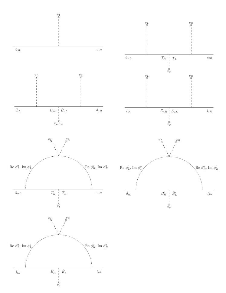
Figure 1: Feynman diagrams contributing to the entries of the SM charged fermion mass matrices. Here, $n=1,2$ and $i,j=1,2,3$.

Figure 2: One-loop Feynman diagram contributing to the Majorana neutrino mass submatrix $\mu$. Here, $n,k=1,2,3$ and $r=1,2$.

Figure 3: Feynman diagram contributing to the Majorana neutrino mass submatrix $\tilde{\mu}$. Here, $i,j,r,s=1,2,3$ and the cross mark $\otimes$ in the internal lines corresponds to the one loop level induced Majorana mass term.

where we have set $\alpha_{1}=\alpha_{2}=0$ to strongly suppress the tree level FCNC in the quark sector. As seen from Eqs. (43), (54) and (65), the exotic heavy vector-like fermions mix with the SM fermions lighter than top quark. The masses of these vector-like fermions are much larger than the scale of breaking of the left-right symmetry $v_{R}\sim\mathcal{O}(10)$ TeV, since the gauge singlet scalars $\eta$, $\sigma$ and $\rho$ are assumed to acquire vacuum expectation values much larger than this scale. Therefore, the charm, bottom and strange quarks, as well as the tau and muon leptons, acquire their masses from the tree-level Universal seesaw mechanism, whereas the first generation SM charged fermions, i.e., the up, down quarks and the electron get one-loop level masses from a radiative seesaw mechanism. Thus, the SM charged fermion mass matrices take the form:

$$\widetilde{M}_{U} = \left(\begin{array}[]{cc}\Delta_{U}-A_{U}M_{\widetilde{T}}^{-1}B_{U}&0_{2\times 1}\\ 0_{1\times 2}&m_{t}\end{array}\right),$$ (68)

$$\widetilde{M}_{D} = \Delta_{D}-A_{D}M_{B}^{-1}B_{D},$$ (69)

$$\widetilde{M}_{E} = \Delta_{E}-A_{E}M_{E}^{-1}B_{E},$$ (70)

where $\Delta_{U}$, $\Delta_{D}$ and $\Delta_{E}$ are the one loop level contributions to the SM charged fermion mass matrices arising from the one-loop Feynman diagrams of Figure 1. It is worth mentioning that the first and second Feynman diagrams of the first row of Figure 1 contribute to the $\left(3,i\right)$ and $\left(n,i\right)$ ($i=1,2,3$ and $n=1,2$) entries of the SM up type quark mass matrix, respectively. The first and the second diagrams from the second row of Figure 1 contribute to the $\left(i,j\right)$ ($i,j=1,2,3$) entries of the SM down type quark and SM charged lepton mass matrices, respectively. Furthermore, the one loop level contributions to the $\left(n,i\right)$ entries of the SM up type quark mass matrix arise from the first diagram of the third row of Figure 1. On the other hand, the second diagram of the third row of Figure 1 generates the one loop level contribution to the $\left(i,j\right)$ entries of the SM down type quark mass matrix. Finally, the last diagram of Figure 1 yields the one loop level contribution to the $\left(i,j\right)$ entries of the SM charged lepton mass matrix. The one loop level contributions to the SM charged fermion mass matrices are given by:

$$\Delta_{U} = \frac{m_{T^{\prime}}}{16\pi^{2}}\left(\begin{array}[]{ccc}w_{1}^{\left(T^{\prime}\right)}r_{1}^{\left(T^{\prime}\right)}&w_{1}^{\left(T^{\prime}\right)}r_{2}^{\left(T^{\prime}\right)}&w_{1}^{\left(T^{\prime}\right)}r_{3}^{\left(T^{\prime}\right)}\\ w_{2}^{\left(T^{\prime}\right)}r_{1}^{\left(T^{\prime}\right)}&w_{2}^{\left(T^{\prime}\right)}r_{2}^{\left(T^{\prime}\right)}&w_{2}^{\left(T^{\prime}\right)}r_{3}^{\left(T^{\prime}\right)}\\ 0&0&0\end{array}\right)$$

$$\times\left\{\left[f\left(m_{S_{1}}^{2},m_{T^{\prime}}^{2}\right)-f\left(m_{S_{2}}^{2},m_{T^{\prime}}^{2}\right)\right]\sin 2\theta_{S}-\left[f\left(m_{P_{1}}^{2},m_{T^{\prime}}^{2}\right)-f\left(m_{P_{2}}^{2},m_{T^{\prime}}^{2}\right)\right]\sin 2\theta_{P}\right\},$$

$$\Delta_{D} = \frac{2m_{B^{\prime}}}{16\pi^{2}}\left(\begin{array}[]{ccc}w_{1}^{\left(B^{\prime}\right)}r_{1}^{\left(B^{\prime}\right)}&w_{1}^{\left(B^{\prime}\right)}r_{2}^{\left(B^{\prime}\right)}&w_{1}^{\left(B^{\prime}\right)}r_{3}^{\left(B^{\prime}\right)}\\ w_{2}^{\left(B^{\prime}\right)}r_{1}^{\left(B^{\prime}\right)}&w_{2}^{\left(B^{\prime}\right)}r_{2}^{\left(B^{\prime}\right)}&w_{2}^{\left(B^{\prime}\right)}r_{3}^{\left(B^{\prime}\right)}\\ 0&0&0\end{array}\right)$$

$$\times\left\{\left[f\left(m_{S_{1}}^{2},m_{B^{\prime}}^{2}\right)-f\left(m_{S_{2}}^{2},m_{B^{\prime}}^{2}\right)\right]\sin 2\theta_{S}-\left[f\left(m_{P_{1}}^{2},m_{B^{\prime}}^{2}\right)-f\left(m_{P_{2}}^{2},m_{B^{\prime}}^{2}\right)\right]\sin 2\theta_{P}\right\},$$

$$\Delta_{E} = \frac{2m_{E^{\prime}}}{16\pi^{2}}\left(\begin{array}[]{ccc}w_{1}^{\left(E^{\prime}\right)}r_{1}^{\left(E^{\prime}\right)}&w_{1}^{\left(E^{\prime}\right)}r_{2}^{\left(E^{\prime}\right)}&w_{1}^{\left(E^{\prime}\right)}r_{3}^{\left(E^{\prime}\right)}\\ w_{2}^{\left(E^{\prime}\right)}r_{1}^{\left(E^{\prime}\right)}&w_{2}^{\left(E^{\prime}\right)}r_{2}^{\left(E^{\prime}\right)}&w_{2}^{\left(E^{\prime}\right)}r_{3}^{\left(E^{\prime}\right)}\\ w_{3}^{\left(E^{\prime}\right)}r_{1}^{\left(E^{\prime}\right)}&w_{3}^{\left(E^{\prime}\right)}r_{2}^{\left(E^{\prime}\right)}&w_{3}^{\left(E^{\prime}\right)}r_{3}^{\left(E^{\prime}\right)}\end{array}\right)$$

$$\times\left\{\left[f\left(m_{S_{1}}^{2},m_{E^{\prime}}^{2}\right)-f\left(m_{S_{2}}^{2},m_{E^{\prime}}^{2}\right)\right]\sin 2\theta_{S}-\left[f\left(m_{P_{1}}^{2},m_{E^{\prime}}^{2}\right)-f\left(m_{P_{2}}^{2},m_{E^{\prime}}^{2}\right)\right]\sin 2\theta_{P}\right\},$$

where $f\left(m_{1},m_{2}\right)$ is given by:

$$f\left(m_{1},m_{2}\right)=\frac{m_{1}^{2}}{m_{1}^{2}-m_{2}^{2}}\ln\left(\frac{m_{1}^{2}}{m_{2}^{2}}\right),$$ (83)

and the physical scalars $S_{1}$, $S_{2}$ and pseudoscalars $P_{1}$ and $P_{2}$ are given by:

$$\left(\begin{array}[]{c}S_{1}\\ S_{2}\end{array}\right)=\left(\begin{array}[]{cc}\cos\theta_{S}&\sin\theta_{S}\\ -\sin\theta_{S}&\cos\theta_{S}\end{array}\right)\left(\begin{array}[]{c}\mathop{\mathrm{R}e}\phi_{L}^{0}\\ \mathop{\mathrm{R}e}\phi_{R}^{0}\end{array}\right),\hskip 28.45274pt\left(\begin{array}[]{c}\ P_{1}\\ P_{2}\end{array}\right)=\left(\begin{array}[]{cc}\cos\theta_{P}&\sin\theta_{P}\\ -\sin\theta_{P}&\cos\theta_{P}\end{array}\right)\left(\begin{array}[]{c}\mathop{\mathrm{I}m}\phi_{L}^{0}\\ \mathop{\mathrm{I}m}\phi_{R}^{0}\end{array}\right).$$ (84)

It is worth mentioning that the SM charged fermion mass hierarchy can be successfully reproduced by having appropriate values for the exotic fermion masses. For instance, to successfully explain the GeV scale value of the bottom quark and tau lepton masses, we have that such masses can be estimated as:

$$m_{b}\sim m_{\tau}\sim\frac{y^{2}v_{L}v_{R}}{m_{F}}$$ (85)

where $m_{\mathrm{F}}$ is the mass scale of the exotic fermions, $y$ the SM fermion-exotic fermion Yukawa coupling and $\lambda$ the quartic scalar coupling. Taking $v_{L}\sim\mathcal{O}\left(100\right)$ GeV, $v_{R}\sim\mathcal{O}\left(10\right)$ TeV, $m_{F}\sim\mathcal{O}\left(100\right)$ TeV and $y\sim\mathcal{O}\left(0.4\right)$, Eq. (85) takes the form $m_{b}\sim m_{\tau}\sim\mathcal{O}\left(1\right)$ GeV, thus showing that our model naturally explains the smallness of the bottom and tau masses with respect to the top quark mass. Furthermore, the hierarchy between the masses of the remaining SM charged fermions lighter than the top quark can be accommodated by having some deviation from the scenario of universality of the Yukawa couplings in both quark and lepton sectors. This would imply some moderate tuning among the Yukawa couplings. However, such a situation is considerably better compared to that of the minimal Left-Right symmetric model, where a significant tuning of the Yukawa couplings is required. In order to find the best fit point that successfully reproduces the SM quark masses and CKM parameters, we proceed to minimize the following $\chi^{2}$ function:

$$\chi^{2}=\sum_{f}\frac{(m_{f}^{\text{th}}-m_{f}^{\text{exp}})^{2}}{\sigma_{f}^{2}}+\frac{(|\mathbf{V}_{12}^{\text{th}}|-|\mathbf{V}_{12}^{\text{exp}}|)^{2}}{\sigma_{12}^{2}}+\frac{(|\mathbf{V}_{23}^{\text{th}}|-|\mathbf{V}_{23}^{\text{exp}}|)^{2}}{\sigma_{23}^{2}}+\frac{(|\mathbf{V}_{13}^{\text{th}}|-|\mathbf{V}_{13}^{\text{exp}}|)^{2}}{\sigma_{13}^{2}}+\frac{(J_{q}^{\text{th}}-J_{q}^{\text{exp}})^{2}}{\sigma_{J}^{2}}\,\;,$$ (86)

where $f=u,c,t,d,s,b$ and $J_{q}$ is the Jarlskog parameter. The experimental values for the quark masses are given by Xing:2020ijf ,

$$\begin{split}m_{u}^{\text{exp}}(M_{Z})&=1.24\pm 0.22\text{MeV}\;,\\ m_{c}^{\text{exp}}(M_{Z})&=0.626\pm 0.020\text{GeV}\;,\\ m_{t}^{\text{exp}}(M_{Z})&=172.9\pm 0.04\text{GeV}\;,\\ m_{d}^{\text{exp}}(M_{Z})&=2.69\pm 0.19\text{MeV}\;,\\ m_{s}^{\text{exp}}(M_{Z})&=53.5\pm 4.6\text{MeV}\;,\\ m_{b}^{\text{exp}}(M_{Z})&=2.86\pm 0.03\text{GeV}\;,\end{split}$$

and the CKM parameters are Zyla:2020zbs

$$\begin{split}|\mathbf{V}_{12}^{\text{exp}}|&=0.22452\pm 0.00044\;,\\ |\mathbf{V}_{23}^{\text{exp}}|&=0.04214\pm 0.00076\;,\\ |\mathbf{V}_{13}^{\text{exp}}|&=0.00365\pm 0.00012\;,\\ J_{q}^{\text{exp}}&=(3.18\pm 0.15)\times 10^{-5}\;.\end{split}$$

The magnitudes of the quark Yukawa couplings are randomly varied in the range $[0.1,1.5]$, whereas their complex phases are ranged between $0$ and $2\pi$. Furthermore, we have fixed $v_{L}=$ $100$GeV and $v_{R}=10$TeV and randomly varied $\theta=\theta_{S}=-\theta_{P}$ in a small range around $\frac{\pi}{3}$. The masses of the vector like quarks and inert scalar mediators are varied in the ranges:

$$0.5\mbox{TeV} \leq m_{S_{1}}=m_{P_{1}}\leq 10\mbox{TeV},\hskip 28.45274pt1.01m_{S_{1}}\leq m_{S_{2}}=m_{P_{2}}\leq 1.03m_{S_{1}},\hskip 28.45274pt1\mbox{TeV}\leq m_{T^{\prime}},m_{B^{\prime}}\leq 10^{3}\mbox{TeV},$$

$$10^{2}\mbox{TeV} \leq m_{B_{1}}\leq 2\times 10^{2}\mbox{TeV},\hskip 25.6073pt10^{2}\frac{m_{b}}{m_{c}}\mbox{TeV}\leq m_{T}\leq 2\times 10^{2}\frac{m_{b}}{m_{c}}\mbox{TeV},\hskip 25.6073pt10^{2}\frac{m_{b}}{m_{s}}\mbox{TeV}\leq m_{B_{2}}\leq 2\times 10^{2}\frac{m_{b}}{m_{s}}\mbox{TeV},\hskip 25.6073pt$$

In the above described range of parameters, we find that the minimization of the $\chi^{2}$ function yields the following benchmark point, consistent with the experimental values of the SM quark masses and CKM parameters:

$$\theta \simeq 85.9^{\circ},\hskip 28.45274ptm_{S_{1}}=m_{P_{1}}\simeq 1.9\mbox{TeV},\hskip 28.45274ptm_{S_{2}}=m_{P_{2}}\simeq 2.1\mbox{TeV},\hskip 28.45274ptv_{L}\simeq 100\mbox{GeV},\hskip 28.45274ptv_{R}\simeq 10\mbox{TeV},$$

$$m_{T} \simeq 583\mbox{TeV},\hskip 25.6073ptm_{T^{\prime}}\simeq 1.1\times 10^{3}\mbox{TeV},\hskip 25.6073ptm_{B_{1}}\simeq 216\mbox{TeV},\hskip 25.6073ptm_{B_{2}}\simeq 9.3\times 10^{3}\mbox{TeV},\hskip 25.6073ptm_{B^{\prime}}\simeq 396\mbox{TeV},$$

$$x_{1}^{\left(T\right)} \simeq 0.24-0.02i,\hskip 28.45274ptx_{2}^{\left(T\right)}\simeq 0.96-0.06i,\hskip 28.45274ptz_{1}^{\left(T\right)}=z_{2}^{\left(T\right)}\simeq-0.16+0.08i,\hskip 28.45274ptx_{12}^{\left(B\right)}\simeq-0.05-0.03i,$$

$$x_{22}^{\left(B\right)} \simeq -0.62-0.06i,\hskip 28.45274ptx_{3}^{\left(B\right)}\simeq 0.07-0.62i,\hskip 28.45274ptz_{11}^{\left(B\right)}\simeq 0.25,\hskip 28.45274ptz_{12}^{\left(B\right)}\simeq 0.49,\hskip 28.45274ptz_{13}^{\left(B\right)}\simeq-0.44,$$

$$z_{21}^{\left(B\right)} \simeq -1.17i,\hskip 28.45274ptz_{22}^{\left(B\right)}\simeq 0.95i,\hskip 28.45274ptz_{23}^{\left(B\right)}\simeq 0.80i,\hskip 28.45274ptw_{1}^{\left(T^{\prime}\right)}\simeq-0.39+0.197i,\hskip 28.45274ptw_{2}^{\left(T^{\prime}\right)}\simeq-0.58+0.29i,$$

$$r_{1}^{\left(T^{\prime}\right)} \simeq -0.154+0.084i,\hskip 28.45274ptr_{2}^{\left(T^{\prime}\right)}\simeq-0.875+0.48i,\hskip 28.45274ptr_{3}^{\left(T^{\prime}\right)}\simeq 0.30-0.16i,\hskip 28.45274ptw_{1}^{\left(B^{\prime}\right)}\simeq 0.12-0.087i,$$

$$w_{2}^{\left(B^{\prime}\right)} \simeq 0.44+0.74i,\hskip 28.45274ptr_{1}^{\left(B^{\prime}\right)}\simeq-0.17-0.98i,\hskip 28.45274ptr_{2}^{\left(B^{\prime}\right)}\simeq-1.22,\hskip 28.45274ptr_{3}^{\left(B^{\prime}\right)}\simeq 1.299+0.698i,$$ (87)

As we can see, the dimensionless quark Yukawa couplings are of order unity with moderate deviations. This shows that the proposed model is able to explain the existing pattern of the observed quark spectrum. The resulting correlations among the heavy exotic quark masses and between the exotic quark masses and the masses $m_{S_{1}}$ and $m_{S_{2}}$ of the inert scalars $S_{1}$ and $S_{2}$ are shown in Figures 4 and 5, respectively, which present the allowed region of parameter space for the seesaw mediator masses, consistent with a successful description of the observed pattern of SM quark masses and CKM parameters. As shown in Figures 4 and 5, the observed SM quark mass and mixing hierarchy can be successfully accounted for, provided that the heavy vector like quark have masses in the ranges $450$ TeV $\lesssim m_{T}\lesssim 700$ TeV, $900$ TeV $\lesssim m_{T^{\prime}}\lesssim 1400$ TeV, $7.5\times 10^{3}$ TeV $\lesssim m_{B_{2}}\lesssim 11\times 10^{3}$ TeV, $300$ TeV $\lesssim m_{T^{\prime}}\lesssim 500$ TeV, wheras the masses of the inert scalars are constrained to be in the ranges $1.4$ TeV $\lesssim m_{S_{1}}\lesssim 2.2$ TeV and $1.7$ TeV $\lesssim m_{S_{2}}\lesssim 2.5$ TeV for $m_{S_{1}}=m_{P_{1}}$ and $m_{S_{2}}=m_{P_{2}}$.

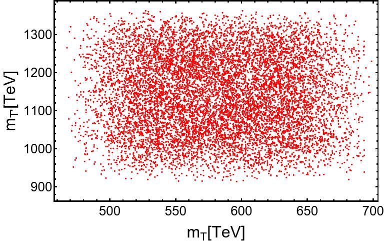
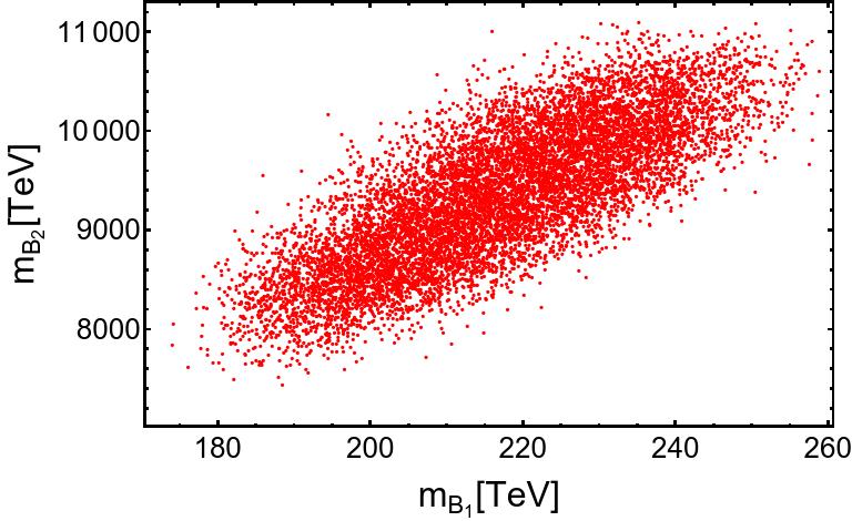
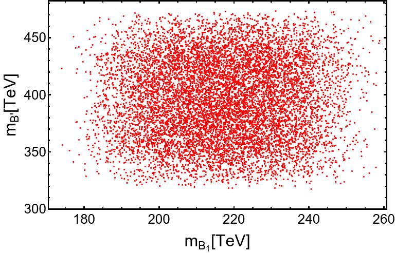
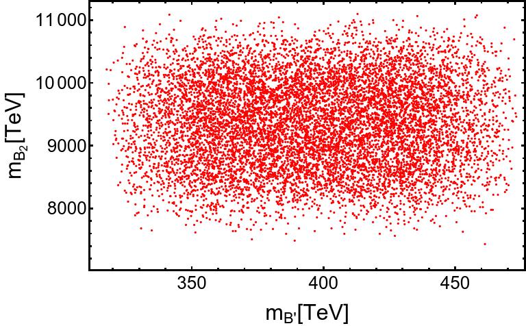
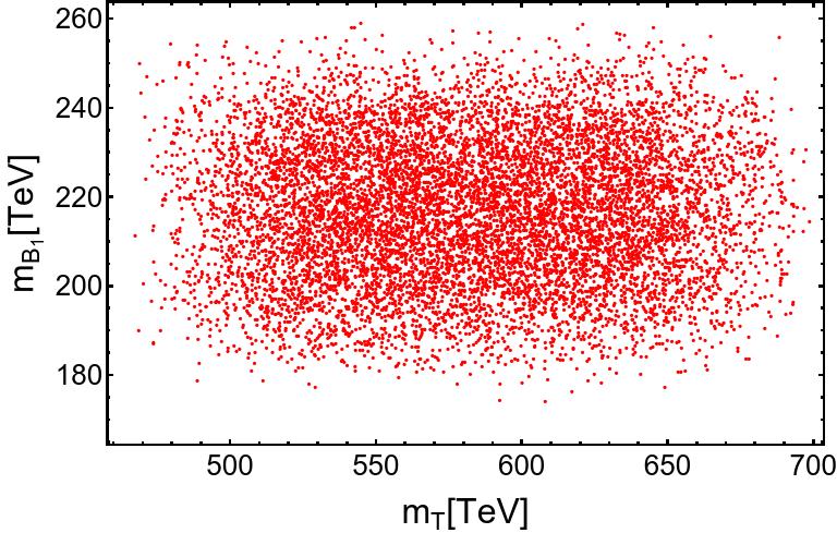
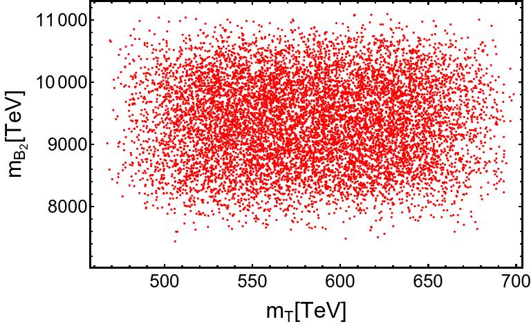
Figure 4: Correlations between the heavy exotic quark masses.

It may seem that the problem of the hierarchies of SM fermions is not solved but simply reparameterized in terms of unknown vector-like fermion masses. However, there are six advantages to this approach. Firstly, the approach is dynamical, since the vector-like masses, which are dynamically generated from Yukawa interactions involving the gauge singlet scalars neutral under the remnant $Z_{2}$ symmetry, are new physical quantities, which could in principle be determined by a future theory. Secondly, it has experimental consequences, since the new vector-like charged exotic fermions and right handed neutrinos can be discovered directly at proton-proton colliders via their production by gluon fusion (for the exotic quarks only) and Drell Yan mechanisms, or indirectly from their loop contributions to certain observables. For instance, the charged exotic vector like leptons, which mediate the Universal seesaw mechanism that produces the SM charged lepton masses, are also crucial for accommodating the experimental values of the muon and electron anomalous magnetic moments, whose magnitudes do not find an explanation within the context of the Standard Model. Thirdly, this approach can also account for the small quark mixing angles, as well as the large lepton mixing angles arising from the neutrino sector. Fourthly, the effective Yukawa couplings are proportional to a product of two other dimensionless couplings, so a small hierarchy in those couplings can yield a quadratically larger hierarchy in the effective couplings. Fifthly, the masses of the light active neutrinos are dynamically generated via a radiative inverse seesaw mechanism at one loop level, thanks to the remnant $Z_{2}$ symmetry arisen from the spontaneous breaking of the $Z_{4}$ symmetry. Sixthly, the remnant $Z_{2}$ symmetry allows for stable scalar and fermionic dark matter candidates. For all these reasons, the approach we follow in this paper is both well motivated and interesting.

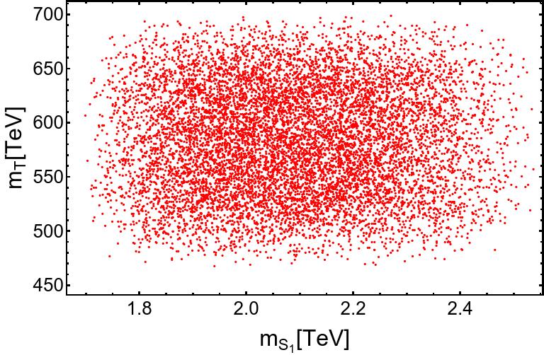
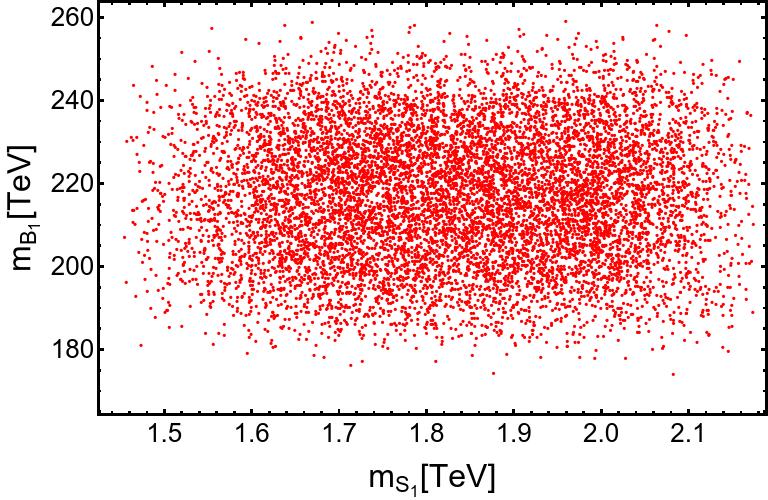
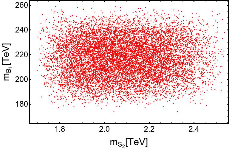
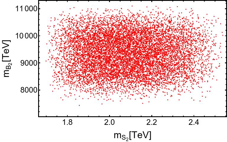
Figure 5: Correlations between the exotic quark masses and the masses $m_{S_{1}}$ and $m_{S_{2}}$ of the inert scalars $S_{1}$ and $S_{2}$, respectively.

Concerning the neutrino sector, we find that the neutrino Yukawa interactions give rise to the following neutrino mass terms:

$$-\mathcal{L}_{mass}^{\left(\nu\right)}=\frac{1}{2}\left(\begin{array}[]{ccc}\overline{\nu_{L}^{C}}&\overline{\nu_{R}}&\overline{N_{R}}\end{array}\right)M_{\nu}\left(\begin{array}[]{c}\nu_{L}\\ \nu_{R}^{C}\\ N_{R}^{C}\end{array}\right)+\mathop{\displaystyle\sum}\limits_{n=1}^{2}\left(m_{\Omega}\right)_{n}\overline{\Omega}_{nR}\Omega_{nR}^{C}+H.c,$$ (88)

where the neutrino mass matrix reads:

$$M_{\nu}=\left(\begin{array}[]{ccc}0_{3\times 3}&m_{\nu D}&0_{3\times 3}\\ m_{\nu D}^{T}&\widetilde{\mu}&M\\ 0_{3\times 3}&M^{T}&\mu\end{array}\right),$$ (89)

and the submatrices are given by:

$$\left(m_{\nu D}\right)_{ij} = y_{ij}^{\left(L\right)}\frac{v_{1}}{\sqrt{2}},\hskip 19.91684pt\hskip 19.91684ptM_{ij}=x_{ij}^{\left(N\right)}\frac{v_{R}}{\sqrt{2}},\hskip 19.91684pt\hskip 19.91684pti,j,n,k=1,2,3,\hskip 19.91684pt\hskip 19.91684ptr=1,2,$$

$$\mu_{nk} = \mathop{\displaystyle\sum}\limits_{r=1}^{2}\frac{x_{nr}^{\left(S\right)}x_{kr}^{\left(S\right)}m_{\Omega_{r}}}{16\pi^{2}}\left[\frac{m_{\varphi_{R}}^{2}}{m_{\varphi_{R}}^{2}-m_{\Omega_{r}}^{2}}\ln\left(\frac{m_{\varphi_{R}}^{2}}{m_{\Omega_{r}}^{2}}\right)-\frac{m_{\varphi_{I}}^{2}}{m_{\varphi_{I}}^{2}-m_{\Omega_{r}}^{2}}\ln\left(\frac{m_{\varphi_{I}}^{2}}{m_{\Omega_{r}}^{2}}\right)\right],\hskip 19.91684pt\hskip 19.91684pt.$$ (90)

The $\mu$ block is generated at one loop level due to the exchange of $\Omega_{rR}$ ($r=1,2$) and $\varphi$ in the internal lines, as shown in Figure 2. To close the corresponding one loop diagram, the following trilinear scalar interaction is needed:

$$V_{\mu}=A\left(\varphi^{\ast}\right)^{2}\sigma,$$ (91)

Furthermore, the $\widetilde{\mu}$ submatrix is generated from the Feynman diagram of Figure 3, which involves the virtual exchange of $\mathop{\mathrm{R}e}\chi_{R}^{0}$, $\mathop{\mathrm{I}m}\chi_{R}^{0}$, $Z^{\prime}$ as well as the one loop level induced Majorana mass term in the internal lines of the loop, in analogy with Pilaftsis:1991ug . The entries of the submatrix $\widetilde{\mu}$ are given by:

$$\widetilde{\mu}_{ij} = \frac{g_{R}^{2}}{16\pi^{2}}\mu_{ij}\frac{m_{Z^{\prime}}^{2}}{m_{Z^{\prime}}^{2}-\mu_{ij}^{2}}\ln\left(\frac{m_{Z^{\prime}}^{2}}{\mu_{ij}^{2}}\right)$$

$$+\mathop{\displaystyle\sum}\limits_{r=1}^{3}\mathop{\displaystyle\sum}\limits_{s=1}^{3}\frac{x_{ri}^{\left(N\right)}x_{sj}^{\left(N\right)}}{16\pi^{2}}\mu_{rs}\left[\frac{m_{\chi_{R}^{0}}^{2}}{m_{\chi_{R}^{0}}^{2}-\left|\mu_{rs}\right|^{2}}\ln\left(\frac{m_{\chi_{R}^{0}}^{2}}{\left|\mu_{rs}\right|^{2}}\right)-\frac{m_{\chi_{I}^{0}}^{2}}{m_{\chi_{I}^{0}}^{2}-\left|\mu_{rs}\right|^{2}}\ln\left(\frac{m_{\chi_{I}^{0}}^{2}}{\left|\mu_{rs}\right|^{2}}\right)\right],$$

Then, as follows from Eq. (III), we have $\left|\widetilde{\mu}_{ij}\right|<<\left|\mu_{ij}\right|$ ($i,j=1,2,3$), since the entries of the $\widetilde{\mu}$ submatrix are much smaller than the entries of the $\mu$ submatrix, by at least two orders of magnitude.

The light active masses arise from an inverse seesaw mechanism and the physical neutrino mass matrices are:

$$\widetilde{\mathbf{M}}_{\nu} = m_{\nu D}\left(M^{T}\right)^{-1}\mu M^{-1}m_{\nu D}^{T},\hskip 19.91684pt$$ (93)

$$\mathbf{M}_{\nu}^{\left(1\right)} = -\frac{1}{2}\left(M+M^{T}\right)+\frac{1}{2}\left(\mu+\widetilde{\mu}\right),\hskip 19.91684pt$$ (94)

$$\mathbf{M}_{\nu}^{\left(2\right)} = \frac{1}{2}\left(M+M^{T}\right)+\frac{1}{2}\left(\mu+\widetilde{\mu}\right).$$ (95)

where $M_{\nu}^{(1)}$ corresponds to the mass matrix for light active neutrinos $\nu_{a}$ ($a=1,2,3$), whereas $M_{\nu}^{(2)}$ and $M_{\nu}^{(3)}$ are the mass matrices for sterile neutrinos ($N_{a}^{-},N_{a}^{+}$) which are superpositions of mostly $\nu_{aR}$ and $N_{aR}$ as $N_{a}^{\pm}\sim\frac{1}{\sqrt{2}}\left(\nu_{aR}\mp N_{aR}\right)$. In the limit $\mu\rightarrow 0$, which corresponds to unbroken lepton number, the light active neutrinos become massless. The smallness of the $\mu$ and $\widetilde{\mu}$ parameters is responsible for a small mass splitting between the three pairs of sterile neutrinos, thus implying that the sterile neutrinos form pseudo-Dirac pairs. The full neutrino mass matrix given by Eq. (89) can be diagonalized by the following rotation matrix Catano:2012kw :

$$\mathbb{R}=\begin{pmatrix}\mathbf{R}_{\nu}&\mathbf{R}_{1}\mathbf{R}_{M}^{\left(1\right)}&\mathbf{R}_{2}\mathbf{R}_{M}^{\left(2\right)}\\ -\frac{(\mathbf{R}_{1}^{\dagger}+\mathbf{R}_{2}^{\dagger})}{\sqrt{2}}\mathbf{R}_{\nu}&\frac{(1-\mathbf{S})}{\sqrt{2}}\mathbf{R}_{M}^{\left(1\right)}&\frac{(1+\mathbf{S})}{\sqrt{2}}\mathbf{R}_{M}^{\left(2\right)}\\ -\frac{(\mathbf{R}_{1}^{\dagger}-\mathbf{R}_{2}^{\dagger})}{\sqrt{2}}\mathbf{R}_{\nu}&\frac{(-1-\mathbf{S})}{\sqrt{2}}\mathbf{R}_{M}^{\left(1\right)}&\frac{(1-\mathbf{S})}{\sqrt{2}}\mathbf{R}_{M}^{\left(2\right)}\end{pmatrix},$$ (96)

where

$$\mathbf{S}=-\frac{1}{4}M^{-1}\mu,\hskip 28.45274pt\hskip 28.45274pt\mathbf{R}_{1}\simeq\mathbf{R}_{2}\simeq\frac{1}{\sqrt{2}}m_{\nu D}^{\ast}M^{-1}.$$ (97)

Notice that the physical neutrino spectrum is composed of three light active neutrinos and six exotic neutrinos. The exotic neutrinos are pseudo-Dirac, with masses $\sim\pm\frac{1}{2}\left(M+M^{T}\right)$ and a small splitting $\mu$. Furthermore, $\mathbf{R}_{\nu}$, $\mathbf{R}_{M}^{\left(1\right)}$ and $\mathbf{R}_{M}^{\left(2\right)}$ are the rotation matrices which diagonalize $\widetilde{\mathbf{M}}_{\nu}$, $\mathbf{M}_{\nu}^{\left(1\right)}$ and $\mathbf{M}_{\nu}^{\left(2\right)}$, respectively.

On the other hand, using Eq. (96) we find that the neutrino fields $\nu_{L}=\left(\nu_{1L},\nu_{2L},\nu_{3L}\right)^{T}$, $\nu_{R}^{C}=\left(\nu_{1R}^{C},\nu_{2R}^{C},\nu_{3R}^{C}\right)$ and $N_{R}^{C}=\left(N_{1R}^{C},N_{2R}^{C},N_{3R}^{C}\right)$ are related with the physical neutrino fields by the following relations:

$$\left(\begin{array}[]{c}\nu_{L}\\ \nu_{R}^{C}\\ N_{R}^{C}\end{array}\right)=\mathbb{R}\Psi_{L}\simeq\begin{pmatrix}\mathbf{R}_{\nu}&\mathbf{R}_{1}\mathbf{R}_{M}^{\left(1\right)}&\mathbf{R}_{2}\mathbf{R}_{M}^{\left(2\right)}\\ -\frac{(\mathbf{R}_{1}^{\dagger}+\mathbf{R}_{2}^{\dagger})}{\sqrt{2}}\mathbf{R}_{\nu}&\frac{(1-\mathbf{S})}{\sqrt{2}}\mathbf{R}_{M}^{\left(1\right)}&\frac{(1+\mathbf{S})}{\sqrt{2}}\mathbf{R}_{M}^{\left(2\right)}\\ -\frac{(\mathbf{R}_{1}^{\dagger}-\mathbf{R}_{2}^{\dagger})}{\sqrt{2}}\mathbf{R}_{\nu}&\frac{(-1-\mathbf{S})}{\sqrt{2}}\mathbf{R}_{M}^{\left(1\right)}&\frac{(1-\mathbf{S})}{\sqrt{2}}\mathbf{R}_{M}^{\left(2\right)}\end{pmatrix}\left(\begin{array}[]{c}\Psi_{L}^{\left(1\right)}\\ \Psi_{L}^{\left(2\right)}\\ \Psi_{L}^{\left(3\right)}\end{array}\right),\hskip 14.22636pt\hskip 14.22636pt\hskip 14.22636pt\hskip 14.22636pt\Psi_{L}=\left(\begin{array}[]{c}\Psi_{L}^{\left(1\right)}\\ \Psi_{L}^{\left(2\right)}\\ \Psi_{L}^{\left(3\right)}\end{array}\right),$$ (98)

where $\Psi_{jL}^{\left(1\right)}$, $\Psi_{jL}^{\left(2\right)}=N_{j}^{+}$ and $\Psi_{jL}^{\left(3\right)}=N_{j}^{-}$ ($j=1,2,3$) are the three active neutrinos and six exotic neutrinos, respectively.

Finally to close this section we provide a discussion about collider signatures of exotic fermions of our model. From the Yukawa interactions it follows that the charged exotic fermions have mixing mass terms with the SM charged fermions, which allows the former to decay into any of the scalars of the model and SM charged fermions. These heavy charged exotic fermions can be produced in association with the charged fermions and can be pair produced as well at the LHC via gluon fusion (for the exotic quarks only) and Drell Yan mechanism. Consequently, observing an excess of events in the multijet and multilepton final state can be a signal of support of this model at the LHC. Regarding the sterile neutrino sector, it is worth mentioning that the sterile neutrinos can be produced at the LHC in association with a SM charged lepton, via quark-antiquark annihilation mediated by a $W^{\prime}$ gauge boson. The corresponding total cross section for the process $pp\rightarrow W^{\prime}\rightarrow lN_{a}^{\pm}$ $(a=1,2,3)$ will be sizeable provided that $m_{W^{\prime}}>m_{N_{a}^{\pm}}$, which implies that in the $s$-channel the $W^{\prime}$ gauge boson is on its mass shell. Furthermore, in our model the sterile neutrinos have the following two body decay modes: $N_{a}^{\pm}\rightarrow l_{i}^{\pm}W^{\mp}$, $N_{a}^{\pm}\rightarrow\nu_{i}Z$ and $N_{a}^{\pm}\rightarrow\nu_{i}S$ (where $i=1,2,3$ is a flavor index and $S$ correponds to any of the scalars of our model lighter than the sterile neutrinos), which are suppressed by the small active-sterile neutrino mixing angle, taken to fullfill $\theta\sim\mathcal{O}(10^{-3})$, in order to keep charged have lepton flavor violating decays well below their current experimental upper limit and at the same time successfully comply with the constraints arising from the unitarity Abada:2018nio ; Fernandez-Martinez:2016lgt . Furthermore the heavy sterile neutrinos $N_{a}^{\pm}$ can decay via off-shell gauge bosons via the following modes: $N_{a}^{\pm}\rightarrow l_{i}^{+}l_{j}^{-}\nu_{k}$, $N_{a}^{\pm}\rightarrow l_{i}^{-}u_{j}\bar{d}_{k}$, $N_{a}^{\pm}\rightarrow b\bar{b}\nu_{k}$ (where $i,j,k=1,2,3$ are flavor indices). Consequently, the heavy sterile neutrino can be detected the LHC via the observation of an excess of events with respect to the SM background in a final state composed of a pair of opposite sign charged leptons plus two jets. This signal of a pair of opposite sign charged leptons plus two jets arising from the decay of sterile neutrinos via an offshell $W^{\prime}$ gauge boson features a much lower SM background than the ones arising from the pair production and decays of sterile neutrinos, thus making the sterile neutrino much easier to detect at the LHC in left-right symmetric models than in models having only an extra $U^{\prime}(1)$ symmetry AguilarSaavedra:2012fu ; Das:2012ii . Studies of inverse seesaw neutrino signatures at colliders as well as the production of heavy neutrinos at the LHC are carried out in Refs. Dev:2009aw ; BhupalDev:2012zg ; Das:2012ze ; AguilarSaavedra:2012fu ; Das:2012ii ; Dev:2013oxa ; Das:2014jxa ; Das:2016hof ; Das:2017gke ; Das:2017nvm ; Das:2017zjc ; Das:2017rsu ; Das:2018usr ; Das:2018hph ; Bhardwaj:2018lma ; Helo:2018rll ; Pascoli:2018heg . A comprehensive study of the exotic fermion production at the LHC and the exotic fermion decay modes is beyond the scope of this work and is left for future studies.

IV Charged lepton flavor violation

In this section we will discuss the implications of the model in charged lepton flavor violation. As mentioned in the previous section, the sterile neutrino spectrum of the model is composed of six nearly degenerate heavy neutrinos. These sterile neutrinos, together with the heavy $W^{\prime}$ gauge boson, induce the $l_{i}\rightarrow l_{j}\gamma$ decay at one loop level, whose Branching ratio is given by: Ilakovac:1994kj ; Deppisch:2004fa ; Lindner:2016bgg :

$$Br\left(l_{i}\rightarrow l_{j}\gamma\right) = \frac{\alpha_{W}^{3}s_{W}^{2}m_{l_{i}}^{5}\kappa^{2}}{256\pi^{2}m_{W^{\prime}}^{4}\Gamma_{i}}\mathop{\displaystyle\sum}\limits_{r=1}^{3}\left|G\left(\frac{m_{N_{r}}^{2}}{m_{W^{\prime}}^{2}}\right)\right|^{2},\hskip 14.22636pt\hskip 14.22636pt\hskip 14.22636ptG\left(x\right)=-\frac{2x^{3}+5x^{2}-x}{4\left(1-x\right)^{2}}-\frac{3x^{3}}{2\left(1-x\right)^{4}}\ln x,$$

$$\kappa = \left|\mathop{\displaystyle\sum}\limits_{k=1}^{3}\left(V_{lL}^{\dagger}\right)_{ik}\left(V_{lL}^{\dagger}\right)_{jk}\right|,$$ (99)

where the one loop level contribution arising from the $W$ gauge boson exchange has been neglected, because it is suppressed by the quartic power of the active-sterile neutrino mixing angle $\theta$, assumed to be of the order of $10^{-3}$, for sterile neutrino masses of about $1$ TeV. It has been shown in Ref. Deppisch:2013cya that for such mixing angle the contribution of the $W$ gauge boson to the branching ratio for the $\mu\rightarrow e\gamma$ decay rate takes values of the order of $10^{-16}$, which corresponds to three orders of magnitude below its experimental upper limit of $4.2\times 10^{-13}$. Thus, in this work we only consider the dominant $W^{\prime}$ contribution to the $\mu\rightarrow e\gamma$ decay rate. Furthermore, there will be additional contributions to the $\mu\rightarrow e\gamma$ decay, arising from the virtual exchange of electrically neutral scalars and charged exotic leptons. We have numerically checked that this contribution is close to $10^{-13}$ for charged exotic leptons with masses $m_{E}\sim\mathcal{O}\left(100\right)$ TeV and flavor violating Yukawa couplings around $10^{-3}$. In order to simplify our analysis, we will consider a benchmark scenario where the couplings of the lepton violating scalar interactions are much lower than $10^{-3}$, thus allowing us to consider the $\mu\rightarrow e\gamma$ decay as mainly arising from the $W^{\prime}$ and heavy neutrino virtual exchange. Furthermore, in our analysis we consider the simplified scenario of degenerate heavy neutrinos with a common mass $m_{N}$ and we also set $g_{R}=g$ and $\kappa=10^{-2}$, which corresponds to off-diagonal elements of $V_{lL}$ left handed leptonic rotation matrix of the order of $0.1$.

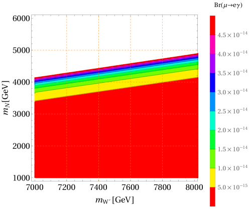
Figure 6: Allowed parameter space in the $m_{W^{\prime}}-m_{N}$ plane consistent with the LFV constraints.

Figure 6 shows the allowed parameter space in the $m_{W^{\prime}}-m_{N}$ plane, consistent with the constraints arising from charged lepton flavor violating decays. The $W^{\prime}$ gauge boson and the sterile neutrino masses have been taken to be in the ranges $7$ TeV$\lesssim m_{W^{\prime}}\lesssim 10$ TeV and $1$ TeV$\lesssim m_{N}\lesssim 10$ TeV, respectively. As seen from Figure 6, the $\mu\rightarrow e\gamma$ decay branching ratio reach values of the order of $10^{-14}$ and lower, which are below its experimental upper limit of $4.2\times 10^{-13}$ and are within the reach of future experimental sensitivity, in the allowed model parameter space. In the region of parameter space consistent with $\mu\rightarrow e\gamma$ decay rate constraints, the maximum obtained branching ratios for the $\tau\rightarrow\mu\gamma$ and $\tau\rightarrow e\gamma$ decays can reach values below their corresponding upper experimental bounds of $4.4\times 10^{-8}$ and $3.3\times 10^{-8}$, respectively. Consequently, our model is compatible with the current charged lepton flavor violating decay constraints.

On the other hand, the Effective Lagrangian approach for describing LFV processes, used in Kuno:1999jp , in the regime of low momentum limit, where the off-shell contributions from photon exchange are negligible with respect to the contributions arising from real photon emission, imply that the dipole operators shown in Ref. Kuno:1999jp will dominate the Lepton Flavor Violating (LFV) transitions $\mu\rightarrow 3e$, $\mu{\text{Al}}\rightarrow e{\text{Al and }}\mu{\text{Ti}}\rightarrow e{\text{T}}$, yielding the following relations Kuno:1999jp ; Lindner:2016bgg :

$${\text{Br}}\left(\mu\rightarrow 3e\right)\simeq\frac{1}{160}{\text{Br}}\left(\mu\rightarrow e\gamma\right),\hskip 28.45274pt{\text{CR}}\left(\mu{\text{Ti}}\rightarrow e{\text{Ti}}\right)\simeq\frac{1}{200}{\text{Br}}\left(\mu\rightarrow e\gamma\right),\hskip 28.45274pt{\text{CR}}\left(\mu{\text{Al}}\rightarrow e{\text{Al}}\right)\simeq\frac{1}{350}{\text{Br}}\left(\mu\rightarrow e\gamma\right)$$ (100)

where the $\mu^{-}-e^{-}$ conversion ratio is defined Lindner:2016bgg as follows:

$${\text{CR}}\left(\mu-e\right)=\frac{\Gamma\left(\mu^{-}+{\text{Nucleus}}\left(A,Z\right)\rightarrow e^{-}+{\text{Nucleus}}\left(A,Z\right)\right)}{\Gamma\left(\mu^{-}+{\text{Nucleus}}\left(A,Z\right)\rightarrow\nu_{\mu}+{\text{Nucleus}}\left(A,Z-1\right)\right)}$$ (101)

Consequently, for our model we expect that the resulting rates for the LFV transitions $\mu\rightarrow 3e$, $\mu{\text{Al}}\rightarrow e{\text{Al and }}\mu{\text{Ti}}\rightarrow e{\text{T}}$ will be of the order of $10^{-16}$, i.e, two orders of magnitude lower than the obtained rate for the $\mu\rightarrow e\gamma$ decay, implying that in our model the corresponding values are below their current experimental bounds of about $10^{-12}$ for these LFV transitions.

V Leptogenesis

In this section we will analyze the implications of our model in leptogenesis. In our analysis of leptogenesis we follow the approach of Ref. Blanchet:2009kk . To simplify our analysis, we work in the basis where the SM charged lepton mass matrix is diagonal, assume that $y^{(L)}$ and $x^{(N)}$ are diagonal matrices and consider the scenario where $\left|y_{11}^{(L)}\right|\ll\left|y_{22}^{(L)}\right|,\left|y_{33}^{(L)}\right|$ and $\left|x_{11}^{(N)}\right|\ll\left|x_{22}^{(N)}\right|,\left|x_{33}^{(N)}\right|$. In that scenario only the first generation of pseudo-Dirac fermions $N_{a}^{\pm}$, i.e, $N_{1}^{\pm}$ will be much lighter than the second and third generation ones. This implies that the decay of $N_{1}^{\pm}$ provides the dominant contribution to the Baryon asymmetry of the Universe (BAU), whereas the decays of the heavier pseudo-Dirac fermions $N_{2}^{\pm}$ and $N_{3}^{\pm}$ will give subleading contributions to the $B-L$ asymmetry. This is due to the fact that the lepton asymmetry generated by the decays of the heavier pseudo-Dirac pairs $N_{2}^{\pm}$ and $N_{3}^{\pm}$ gets washed out very quickly, yielding a very small impact on the lepton asymmetry produced by the decay of the lightest pair $N_{1}^{\pm}$, as discussed in Ref. Blanchet:2009kk . We are considering the scenario of diagonal $y^{(L)}$ matrix in order to suppress tree level FCNCs in the charged lepton sector. We also take the initial temperature larger than the mass $m_{{N^{\pm}}}$ of the lightest pair of pseudo-Dirac fermions $N_{1}^{\pm}=N^{\pm}$. Within this minimal scenario, the Boltzmann equations take the form Buchmuller:2004nz :

$$\frac{dN_{{N_{1}^{\pm}}}\left(z\right)}{dz} = -\left[D\left(z\right)+S\left(z\right)\right]\left[N_{{N_{1}^{\pm}}}\left(z\right)-N_{{N_{1}^{\pm}}}^{eq}\left(z\right)\right],$$

$$\frac{dN_{N_{B-L}}\left(z\right)}{dz} = -\varepsilon_{\pm}D\left(z\right)\left[N_{{N_{1}^{\pm}}}\left(z\right)-N_{{N_{1}^{\pm}}}^{eq}\left(z\right)\right]-W\left(z\right)N_{N_{B-L}}\left(z\right),$$ (102)

where $z=\frac{m_{{N_{1}^{\pm}}}}{T}$, whereas $N_{{N_{1}^{\pm}}}$ and $N_{N_{B-L}}$ are the number density and the amount of $B-L$ asymmetry, respectively. Here $\varepsilon_{\pm}$ are the lepton asymmetry parameters, which are induced by the $N^{\pm}$ decay processes and have the following form Covi:1996wh ; Rangarajan:1999kt ; Gu:2010xc ; Pilaftsis:1997jf :

$$\varepsilon_{\pm} = \mathop{\displaystyle\sum}\limits_{i=1}^{3}\mathop{\displaystyle\sum}\limits_{r=1}^{2}\frac{\left[\Gamma\left(N_{\pm}\rightarrow l_{i}H_{r}^{+}\right)-\Gamma\left(N_{\pm}\rightarrow\bar{l}_{i}H_{r}^{-}\right)\right]}{\left[\Gamma\left(N_{\pm}\rightarrow l_{i}H_{r}^{+}\right)+\Gamma\left(N_{\pm}\rightarrow\bar{l}_{i}H_{r}^{-}\right)\right]}+\mathop{\displaystyle\sum}\limits_{i=1}^{3}\frac{\left[\Gamma\left(N_{\pm}\rightarrow h\nu_{i}\right)-\Gamma\left(N_{\pm}\rightarrow h\nu_{i}\right)\right]}{\left[\Gamma\left(N_{\pm}\rightarrow h\nu_{i}\right)+\Gamma\left(N_{\pm}\rightarrow h\nu_{i}\right)\right]}$$ (103)

$$\simeq \frac{\mathop{\mathrm{I}m}\left\{\left(\left[\left(y_{N_{+}}\right)^{\dagger}\left(y_{N_{-}}\right)\right]^{2}\right)_{11}\right\}}{8\pi A_{\pm}}\frac{r}{r^{2}+\frac{\Gamma_{\pm}^{2}}{m_{N_{\pm}}^{2}}},$$

with:

$$r = \frac{m_{N_{+}}^{2}-m_{N_{-}}^{2}}{m_{N_{+}}m_{N_{-}}},\hskip 19.91684pt\hskip 19.91684ptA_{\pm}=\left[\left(y_{N_{\pm}}\right)^{\dagger}y_{N_{\pm}}\right]_{11},\hskip 19.91684pt\hskip 19.91684pt\Gamma_{\pm}=\frac{A_{\pm}m_{N_{\pm}}}{8\pi},$$

$$y_{N_{\pm}} = \frac{y^{\left(L\right)}}{\sqrt{2}}\left(1\mp S\right)=\frac{y^{\left(L\right)}}{\sqrt{2}}\left[1\pm\frac{1}{4}M^{-1}\left(\mu+\widetilde{\mu}\right)\right],$$ (104)

where we have assumed that the exotic leptonic fields $E_{nR}$, $E^{\prime}$ and $\Omega_{nR}$ ($n=1,2$) are heavier than the lightest pseudo-Dirac fermions $N_{1}^{\pm}=N^{\pm}$.

On the other hand, it is worth mentioning that $N_{N_{1}^{\pm}}$ and $N_{N_{B-L}}$ are computed in a portion of comoving volume that contains one photon at temperatures much larger than $m_{{N_{1}^{\pm}}}$, thus implying that $N_{{N_{1}^{\pm}}}^{eq}\left(z<<1\right)=\frac{3}{4}$ Buchmuller:2004nz . Besides that, $D\left(z\right)$, $S\left(z\right)$ and $W\left(z\right)$, are the thermally averaged rates corresponding to the decays of ${N_{1}^{\pm}}$, to the scattering processes and to the inverse decays, respectively. These thermally averaged rates are given by:

$$D\left(z\right) = D\left(z\right)_{N_{1}}+D_{N_{1}}^{\left(W^{\prime}\right)}\left(z\right),\hskip 19.91684pt\hskip 19.91684pt{S\left(z\right)=S_{Z^{\prime}}\left(z\right)+}S_{W^{\prime}}\left(z\right),$$ (105)

$$W\left(z\right) = W_{N_{1}}^{ID}\left(z\right)+W_{N_{1}}^{ID\left(W^{\prime}\right)}\left(z\right),$$ (106)

where $D\left(z\right)_{N_{1}}$ is the thermally averaged rate associated with the two body decays $N_{1}^{\pm}\rightarrow l_{i}H{{}_{r}^{+}}$ ($r=1,2$), $N_{1}^{\pm}\rightarrow\nu_{i}h$ ($i=1,2,3$) whereas $D_{N_{1}}^{\left(W^{\prime}\right)}\left(z\right)$ corresponds to the thermally averaged rate arising from the $W^{\prime}$ mediated three body decay $N_{1}^{\pm}\rightarrow l_{i}^{-}u_{j}\bar{d}_{k}$ ($i,j,k=1,2,3$). Furthermore, $S_{Z^{\prime}}\left(z\right)$ is the thermally averaged rate arising from the $Z^{\prime}$ mediated scattering processes $N_{1}^{\pm}N_{1}^{\pm}\longleftrightarrow l_{i}\overline{l}_{j}$ ($i,j=1,2,3$), $N_{1}^{\pm}N_{1}^{\pm}\longleftrightarrow u_{i}\overline{u}_{j}$ and $N_{1}^{\pm}N_{1}^{\pm}\longleftrightarrow d_{i}\overline{d}_{j}$, whereas the thermally averaged rate $S_{W^{\prime}}\left(z\right)$ is caused by the $W^{\prime}$ mediated processes $N_{1}^{\pm}$$l_{iR}\longleftrightarrow\overline{u}_{jR}d_{kR}$, $N_{1}^{\pm}\overline{u}_{iR}\longleftrightarrow l_{jR}\overline{d}_{kR}$, $N_{1}^{\pm}d$${}_{iR}\longleftrightarrow l_{jR}u_{kR}$ ($i,j,k=1,2,3$). In addition, $W_{N_{1}}^{ID}\left(z\right)$ and $W_{N_{1}}^{ID\left(W^{\prime}\right)}\left(z\right)$ are the thermally averaged rates arising from the inverse two and three body decays of $N_{1}^{\pm}$, respectively. The above mentioned thermally averaged rates are given by Plumacher:1996kc ; Buchmuller:2004nz ; Cosme:2004xs ; Frere:2008ct ; Blanchet:2010kw ; Dolan:2018qpy :

$$D\left(z\right)_{N_{1}} = \frac{\Gamma_{D}}{H\left(z=1\right)z}=Kz\frac{\mathcal{K}_{1}\left(z\right)}{\mathcal{K}_{2}\left(z\right)},\hskip 19.91684pt\hskip 19.91684ptW_{N_{1}}^{ID}\left(z\right)=\frac{1}{2}\frac{\Gamma_{ID}\left(z\right)}{H\left(z\right)z}=\frac{1}{2}\frac{\Gamma_{D}\left(z\right)}{H\left(z\right)z}\frac{N^{eq}\left(z\right)}{N_{l}}=\frac{1}{4}K\mathcal{K}_{1}\left(z\right)z^{3},$$

$$\Gamma_{ID}\left(z\right) = \Gamma_{D}\left(z\right)\frac{N^{eq}\left(z\right)}{N_{l}^{eq}},\hskip 19.91684ptN_{{N_{1}^{\pm}}}^{eq}\left(z\right)=\frac{3}{8}z^{2}\mathcal{K}_{2}\left(z\right),\hskip 19.91684ptN_{l}^{eq}=\frac{3}{4},\hskip 19.91684ptK=\frac{\left[y^{\left(L\right)}\left(y^{\left(L\right)}\right)^{\dagger}\right]_{11}v_{1}^{2}}{2m_{\ast}m_{{{N_{1}^{\pm}}}}},$$

$$D_{N_{1}}^{\left(W^{\prime}\right)}\left(z\right) = \frac{\gamma_{{N_{1}^{\pm}}}^{\left(W_{R}\right)}}{n_{{N_{1}^{\pm}}}^{eq}\left(z\right)H\left(z=1\right)z},\hskip 19.91684ptn_{{N_{1}^{\pm}}}^{eq}\left(z\right)=\frac{3}{4}n_{\gamma}\left(z\right)N_{{N_{1}^{\pm}}}^{eq}\left(z\right)=\frac{9}{64}z^{2}\mathcal{K}_{2}\left(z\right)n_{\gamma}\left(z\right),\hskip 19.91684ptn_{\gamma}=\frac{2\zeta\left(3\right)}{\pi^{2}}T^{3},$$ (107)

$$W_{N_{1}}^{ID\left(W^{\prime}\right)}\left(z\right) = \frac{1}{2}D_{W^{\prime}}\left(z\right)\frac{N^{eq}\left(z\right)}{N_{l}},\hskip 19.91684pt\hskip 19.91684ptS\left(z\right)_{Z^{\prime},W^{\prime}}=\frac{\Gamma_{S}^{\left(Z^{\prime},W^{\prime}\right)}}{H\left(z=1\right)z},\hskip 19.91684pt\hskip 19.91684pt\Gamma_{S}=\frac{\gamma_{{S}}^{\left(Z^{\prime},W^{\prime}\right)}}{n_{{N_{1}^{\pm}}}^{eq}\left(z\right)H\left(z=1\right)z},$$

$$\gamma_{{N_{1}^{\pm}}}^{\left(W^{\prime}\right)} = n_{{N_{1}^{\pm}}}^{eq}\left(z\right)\frac{\mathcal{K}_{1}\left(z\right)}{\mathcal{K}_{2}\left(z\right)}\Gamma_{N}^{\left(W^{\prime}\right)},\hskip 19.91684pt\Gamma_{{N_{1}^{\pm}}}^{\left(W^{\prime}\right)}=\frac{3g_{R}^{4}}{2^{9}\pi^{3}m_{{{N_{1}^{\pm}}}}^{3}}\int_{0}^{m_{{{N_{1}^{\pm}}}}^{2}}ds\frac{m_{{{N_{1}^{\pm}}}}^{6}-3m_{{{N_{1}^{\pm}}}}^{2}s^{2}+2s^{3}}{\left(s-m_{W^{\prime}}^{2}\right)^{2}+m_{W^{\prime}}^{2}\Gamma_{W^{\prime}}^{2}},\hskip 19.91684pt\Gamma_{W^{\prime}}=\frac{g_{R}^{2}}{4\pi}m_{W^{\prime}}^{2},$$

where $\mathcal{K}_{r}\left(z\right)$ ($r=1,2$) is the modified Besel function of the $r$th type, $\Gamma_{{N_{1}^{\pm}}}^{\left(W^{\prime}\right)}$ the total three body decay of ${N_{1}^{\pm}}$, $\Gamma_{W^{\prime}}$ the $W^{\prime}$ total decay width, $n_{{N_{1}^{\pm}}}^{eq}\left(z\right)$ is the right handed equilibrium distribution density, $n_{\gamma}\left(z\right)$ is the number density of photons, $K$ the washout parameter, $m_{\ast}$ the equilibrium neutrino mass, $H\left(z\right)$ the Hubble expansion rate, whereas $\gamma_{S}^{\left(Z^{\prime},W^{\prime}\right)}$, $\gamma_{N_{1}^{\pm}}^{\left(W_{R}\right)}$ are the scattering and decay reaction densities, respectively. The equilibrium neutrino mass $m_{\ast}$ and the Hubble expansion rate $H$ are given by Buchmuller:2004nz :

$$m_{\ast}=\frac{16\pi^{\frac{5}{2}}\sqrt{g_{\ast}}v_{1}^{2}}{3\sqrt{5}M_{P}}=1.08\times 10^{-3}eV,\hskip 19.91684pt\hskip 19.91684ptH=\sqrt{\frac{4\pi^{3}g_{\ast}}{45}}\frac{T^{2}}{M_{P}}=\sqrt{\frac{4\pi^{3}g_{\ast}}{45}}\frac{m_{{{N_{1}^{\pm}}}}^{2}}{z^{2}M_{P}}\simeq 1.66\sqrt{g_{\ast}}\frac{m_{{{N_{1}^{\pm}}}}^{2}}{z^{2}M_{P}},$$

where $g_{\ast}=118$ is the number of effective relativistic degrees of freedom, $M_{Pl}=1.2\times 10^{9}$ GeV is the Planck constant.

Furthermore, the scattering reaction densities $\gamma_{{S}}^{\left(W^{\prime}\right)}$ and $\gamma_{{S}}^{\left(Z^{\prime}\right)}$ are given by:

$$\gamma_{{S}}^{\left(W^{\prime}\right)} = \gamma_{{{N_{1}^{\pm}}l_{iR}\longleftrightarrow\overline{u}_{jR}d_{kR}}}+\gamma_{{{N_{1}^{\pm}}\overline{u}_{iR}\longleftrightarrow l_{jR}\overline{d}_{kR}}}+\gamma_{{{N_{1}^{\pm}d}_{iR}\longleftrightarrow l_{jR}u_{kR}}},$$

$$\gamma_{{S}}^{\left(Z^{\prime}\right)} = \gamma_{{{N_{1}^{\pm}N_{1}^{\pm}}\longleftrightarrow l}_{i}{\overline{l}}_{j}}+\gamma_{{{N_{1}^{\pm}N_{1}^{\pm}}\longleftrightarrow u}_{i}{\overline{u}}_{j}}+\gamma_{{{N_{1}^{\pm}N_{1}^{\pm}}\longleftrightarrow d}_{i}{\overline{d}}_{j}}$$ (108)

where the scattering reaction density for the process $ab\longleftrightarrow cd$ is defined as follows Luty:1992un ; Plumacher:1996kc ; Buchmuller:2004nz ; Cosme:2004xs ; Frere:2008ct ; Blanchet:2010kw ; Dolan:2018qpy :

$$\gamma_{ab\longleftrightarrow cd} = \frac{T}{64\pi^{4}}\int_{s_{\min}}^{\infty}ds\sqrt{s}\widehat{\sigma}_{ab\longleftrightarrow cd}\left(s\right)\mathcal{K}_{1}\left(\frac{\sqrt{s}}{T}\right)=\frac{m_{{{N_{1}^{\pm}}}}^{4}}{64\pi^{4}z}\int_{x_{0}}^{\infty}dx\sqrt{x}\widehat{\sigma}\left(x\right)\mathcal{K}_{1}\left(z\sqrt{x}\right),\hskip 19.91684pt\hskip 19.91684pt$$

$$x = \frac{s}{m_{{{N_{1}^{\pm}}}}^{2}},\hskip 19.91684pt\hskip 19.91684ptx_{0}=\frac{1}{m_{{{N_{1}^{\pm}}}}^{2}}\max\left[\left(m_{a}+m_{b}\right)^{2},\left(m_{c}+m_{d}\right)^{2}\right],\hskip 19.91684pt\hskip 19.91684ptz=\frac{m_{{{N_{1}^{\pm}}}}}{T},$$ (109)

and $\widehat{\sigma}_{ab\longleftrightarrow cd}\left(s\right)$ is the reduced cross section corresponding to the scattering process $ab\longleftrightarrow cd$. In the left-right model under consideration, the relevant reduced cross sections are given by Plumacher:1996kc ; Plumacher:1996kc ; Cosme:2004xs ; Frere:2008ct ; Blanchet:2010kw ; Dolan:2018qpy

$$\widehat{\sigma}_{{{N_{1}^{\pm}}l_{iR}\longleftrightarrow\overline{u}_{jR}d_{kR}}}\left(x\right) = \frac{9g_{R}^{4}}{48\pi x}\frac{1-3x^{2}+2x^{3}}{\left[\left(x-\frac{m_{W^{\prime}}^{2}}{m_{{{N_{1}^{\pm}}}}^{2}}\right)^{2}+\frac{m_{W^{\prime}}^{2}\Gamma_{W^{\prime}}^{2}}{m_{{{N_{1}^{\pm}}}}^{2}}\right]},$$ (110)

$$\widehat{\sigma}_{{{N_{1}^{\pm}}\overline{u}_{iR}\longleftrightarrow l_{jR}\overline{d}_{kR}}}\left(x\right) = \frac{9g_{R}^{4}}{8\pi x}\int_{1-x}^{0}du\frac{\left(x+u\right)\left(x+u-1\right)}{\left(u-\frac{m_{W^{\prime}}^{2}}{m_{{{N_{1}^{\pm}}}}^{2}}\right)^{2}},$$ (111)

$$\widehat{\sigma}_{{{N_{1}^{\pm}d}_{iR}\longleftrightarrow l_{jR}u_{kR}}}\left(x\right) = \frac{9g_{R}^{4}}{8\pi}\frac{m_{{{N_{1}^{\pm}}}}^{2}}{m_{W^{\prime}}^{2}}\frac{\left(1-x\right)^{2}}{x+\frac{m_{W^{\prime}}^{2}}{m_{{{N_{1}^{\pm}}}}^{2}}-1},$$ (112)

$$\widehat{\sigma}_{{{N_{1}^{\pm}N_{1}^{\pm}}\longleftrightarrow l\overline{l}}}\left(x\right)+\gamma_{{{N_{1}^{\pm}N_{1}^{\pm}}\longleftrightarrow u}_{i}{\overline{u}}_{j}}+\gamma_{{{N_{1}^{\pm}N_{1}^{\pm}}\longleftrightarrow d}_{i}{\overline{d}}_{j}} = \frac{13g_{B-L}^{2}}{6\pi}\frac{\sqrt{x\left(x-4\right)^{3}}}{\left(x-\frac{m_{Z^{\prime}}^{2}}{m_{{{N_{1}^{\pm}}}}^{2}}\right)^{2}+\frac{m_{Z^{\prime}}^{2}\Gamma_{Z^{\prime}}^{2}}{m_{{{N_{1}^{\pm}}}}^{2}}},$$ (113)

where $\Gamma_{Z^{\prime}}$ is the total $Z^{\prime}$ decay given by:

$$\Gamma_{Z^{\prime}}=\frac{g_{B-L}^{2}}{24\pi}m_{Z^{\prime}}\left[13+3\left(1-\frac{4m_{{{N_{1}^{\pm}}}}^{2}}{m_{Z^{\prime}}^{2}}\right)^{\frac{3}{2}}\right],$$ (114)

It is worth mentioning that we are not considering the contributions arising from the $t$-channel scattering processes $N_{1}^{\pm}N_{1}^{\pm}$$\longleftrightarrow l_{i}\overline{l}_{j}$ ($i,j=1,2,3$) since its corresponding rates have a very fast decrease for $z$$=\frac{m_{{N_{1}^{\pm}}}}{T}$$>1$, as discussed in Ref. Blanchet:2009kk . Furthermore, we are also not considering contributions arising from $\Delta L=1$ scatterings involving scalars, since they are subleading, as discussed in Ref. Blanchet:2009kk . Moreover, we are not considering scattering processes involving heavy charged exotic fermions, since they are very heavy with masses larger than $100$ TeV (see Eq. (87)) in order to naturally reproduce the SM fermion mass hierarchy.

The numerical solution of the Boltzmann equations allows to determine the amount of $B-L$ asymmetry $N_{B-L}$, and then the baryon to photon ratio, by using the following relation Buchmuller:2004nz ; Frere:2008ct :

$$\eta_{B}=\frac{n_{B}}{n_{\gamma}}=\frac{3}{4}a_{sph}N_{B-L},\hskip 19.91684pt\hskip 19.91684pta_{sph}=\frac{8n_{f}+4n_{H}}{22n_{f}+13n_{H}},$$ (115)

where $a_{sph}$ is the $L$ to $B$ sphaleron conversion rate. Furthermore, $n_{f}$ is the number of fermion families and $n_{H}$ is the number of Higgs doublets.

As shown in Ref. Blanchet:2010kw , the contributions arising from the aforementioned scattering processes, as well as from the inverse decays, are subdominant for temperatures sufficiently lower than the mass $m_{N}$, i.e, $z>>1$, thus implying that the lepton asymmetry mainly arises from the decay of the the lightest pair of pseudo-Dirac fermions $N_{1}^{\pm}$. This is confirmed in Figure 7, which shows the thermally averaged rates corresponding to the decays, scattering and washouts, as a function of $z=\frac{m_{N}}{T}$, where $m_{N}$ is the mass of the lightest pair of pseudo-Dirac fermions $N_{1}^{\pm}=N^{\pm}$ and $T$ the temperature. Here we have set $v_{R}=14$ TeV, $m_{W^{\prime}}=7$ TeV and $m_{Z^{\prime}}=7.2$ TeV. As shown in Figure 7, for $z>\mathcal{O}(10)$ the thermally averaged scattering rate corresponding to the decays is much larger by several orders of magnitudes than the ones associated with the scattering and inverse decays (washouts). Furthermore, it has been shown in Ref. Blanchet:2010kw that the contribution arising from the $W_{R}$ mediated three body decay $N_{1}^{\pm}\rightarrow l_{i}^{-}u_{j}\bar{d}_{k}$ is much smaller than the ones arising from the $N_{1}^{\pm}$$\rightarrow l_{i}H{{}_{r}^{+}}$, $N_{1}^{\pm}$$\rightarrow\nu_{i}h$ decays. On the other hand, if the temperature of the Universe drops below the scale of breaking of the left-right symmetry, the inverse decays producing ${N_{1}^{\pm}}$ fall out of thermal equilibrium, and thermal leptogenesis can take place.

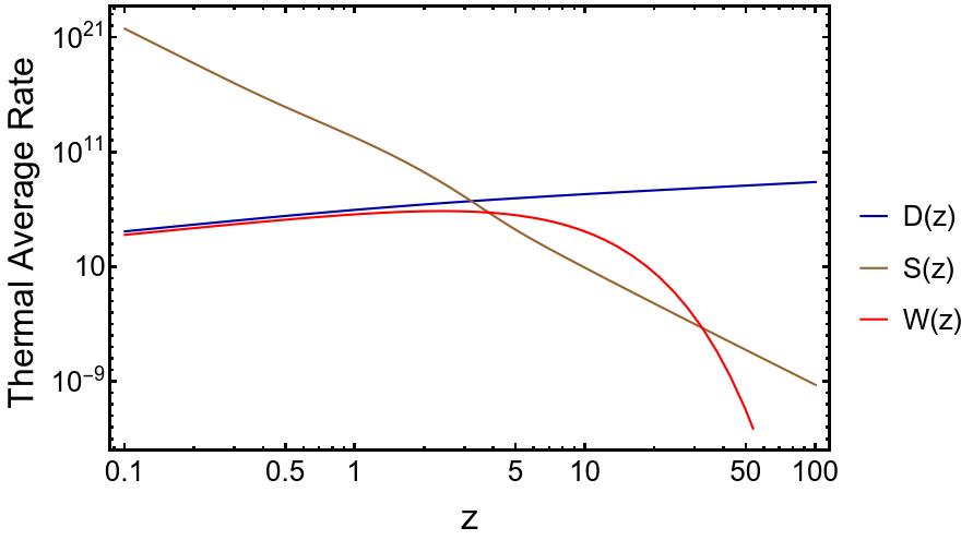
Figure 7: Thermally averaged scattering rates $D\left(z\right)$, $S\left(z\right)$ and $W\left(z\right)$ as functions of $z=\frac{m_{N}}{T}$, with $m_{N}$ the mass of the lightest pair of pseudo-Dirac fermions $N_{1}^{\pm}=N^{\pm}$ and $T$ the temperature. Here we have set $v_{R}=14$ TeV, $m_{W^{\prime}}=7$ TeV and $m_{Z^{\prime}}=7.2$ TeV.

It is worth mentioning that CP violation in the lepton sector, necessary to generate the lepton asymmetry parameter, can arise from complex entries in $y^{\left(L\right)}$, $M$ or $\mu$, as indicated by Eqs. (103) and (104). Furthermore, in order to successfully reproduce the neutrino oscillation experimental data, the submatrix $\mu$, in the basis of diagonal SM charged lepton mass matrix, should have the following form:

$$\mu=M^{T}m_{\nu D}^{-1}\widetilde{\mathbf{M}}_{\nu}\left(m_{\nu D}^{T}\right)^{-1}M=M^{T}m_{\nu D}^{-1}U_{PMNS}\left(\widetilde{\mathbf{M}}_{\nu}\right)_{diag}diag\left(m_{1},m_{2},m_{3}\right)U_{PMNS}^{T}\left(m_{\nu D}^{T}\right)^{-1}M,$$ (116)

where:

$$\left(\widetilde{\mathbf{M}}_{\nu}\right)_{diag}=diag\left(m_{1},m_{2},m_{3}\right)$$ (117)

being $m_{1}$, $m_{2}$ and $m_{3}$ the masses of the light active neutrinos and $U_{PMNS}$ the PMNS leptonic mixing matrix.

The correlations of the baryon asymmetry and the magnitude of the Dirac neutrino Yukawa couplings $y_{11}^{(L)}$ and $y_{22}^{(L)}$ are shown in Figure 8 and 9, respectively. Here we have set $v_{R}=14$ TeV, $m_{W^{\prime}}=7$ TeV, $m_{Z^{\prime}}=7.2$ TeV, $m_{N_{2}^{\pm}}=14$ TeV, $m_{N_{3}^{\pm}}=28$ TeV and $\left|y_{22}^{(L)}\right|=\left|y_{33}^{(L)}\right|=\left|y_{2}^{(L)}\right|$. As shown in Figures 8 and 9, the measured value of the baryon asymmetry of the Universe Zyla:2020zbs :

$$\eta_{B}=\left(6.12\pm 0.04\right)\times 10^{-10}$$ (118)

can be successfully reproduced in the simplified scenario considered in our model, provided that $\left|y_{1}^{(L)}\right|\sim\mathcal{O}\left(10^{-4}\right)$ and $\left|y_{2}^{(L)}\right|\sim\mathcal{O}\left(1\right)$. In our numerical analysis we have found that the baryon asymmetry of the Universe is generated for $z\sim\mathcal{O}\left(10\right)$, which corresponds to temperatures one order of magnitude lower than the mass $m_{N}$ of the lightest pair of pseudo-Dirac fermions $N_{1}^{\pm}=N^{\pm}$. This result is consistent with the one obtained in Ref. Blanchet:2010kw .

The correlation of the baryon asymmetry and the mass $m_{N}$ of the lightest pair of pseudo-Dirac fermions $N_{1}^{\pm}=N^{\pm}$ is shown in Figure 10. As shown in Figures 8, 9 and 10, our model successfully accommodates the experimental value of the baryon asymmetry parameter $\eta_{B}$.

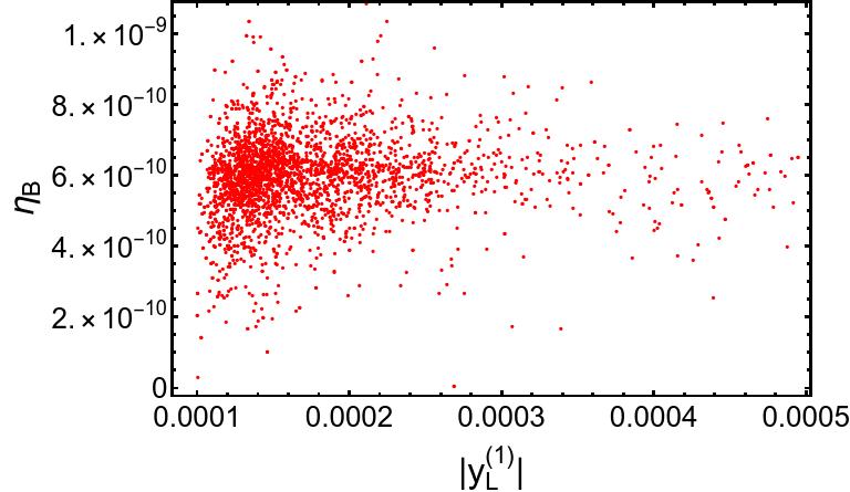
Figure 8: Correlation of the baryon asymmetry and the magnitude of the Dirac neutrino Yukawa coupling $y_{11}^{(L)}$. Here we have set $v_{R}=14$ TeV, $m_{W^{\prime}}=7$ TeV, $m_{Z^{\prime}}=7.2$ TeV, $m_{N_{2}^{\pm}}=14$ TeV, $m_{N_{3}^{\pm}}=28$ TeV and $\left|y_{22}^{(L)}\right|=\left|y_{33}^{(L)}\right|=\left|y_{2}^{(L)}\right|$.

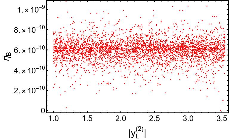
Figure 9: Correlation of the baryon asymmetry and the magnitude of the Dirac neutrino Yukawa coupling $y_{22}^{(L)}$. Here we have set $v_{R}=14$ TeV, $m_{W^{\prime}}=7$ TeV, $m_{Z^{\prime}}=7.2$ TeV, $m_{N_{2}^{\pm}}=14$ TeV, $m_{N_{3}^{\pm}}=28$ TeV and $\left|y_{22}^{(L)}\right|=\left|y_{33}^{(L)}\right|=\left|y_{2}^{(L)}\right|$.

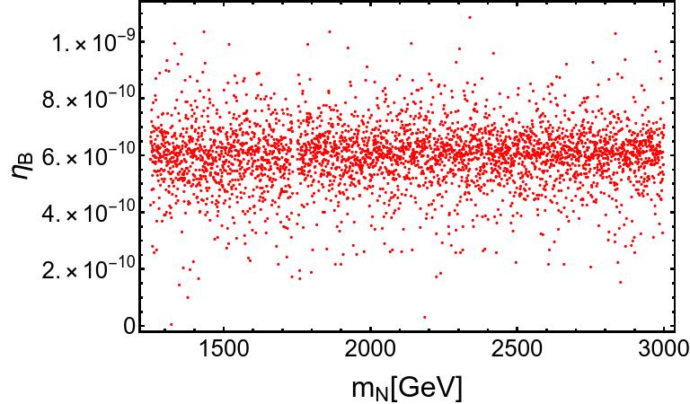
Figure 10: Correlation of the baryon asymmetry and the mass $m_{N}$ of the lightest pair of pseudo-Dirac fermions $N_{1}^{\pm}=N^{\pm}$. Here we have set $v_{R}=14$ TeV, $m_{W^{\prime}}=7$ TeV, $m_{Z^{\prime}}=7.2$ TeV, $m_{N_{2}^{\pm}}=14$ TeV, $m_{N_{3}^{\pm}}=28$ TeV and $\left|y_{22}^{(L)}\right|=\left|y_{33}^{(L)}\right|=\left|y_{2}^{(L)}\right|$

VI The simplified scalar potential

In order to simplify our analysis, we will consider a bechmark scenario where the singlet real scalar fields $\sigma$, $\eta$ and $\rho$ will not feature mixings with the neutral components of the $\Phi$, $\chi_{L}$ and $\chi_{R}$ scalars. Furthermore, for the sake of simplicity, in our bechmark scenario we do not consider the trilinear terms $A_{1}(\chi_{R}^{\dagger}\phi_{R})\varphi$ and $A_{2}(\chi_{L}^{\dagger}\phi_{L})\varphi$ that will give rise to mixings of the gauge singlet scalar field $\varphi$ with the $\phi_{L}$ and $\phi_{R}$ scalars. The justification of the benchmark scenario under consideration arises from the fact that such gauge singlet scalars $\sigma$, $\eta$ and $\rho$ are assumed to acquire vacuum expectation values much larger than the scale of breaking of the left-right symmetry, thus allowing to neglect the mixings of these fields with the $\Phi$, $\chi_{L}$ and $\chi_{R}$ scalars and to treat their scalar potentials independently. Let us note that the mixing angles between those fields are suppressed by the ratios of their VEVs, as follows from the method of recursive expansion of Ref. Grimus:2000vj . The scalar potential for the $\Phi$, $\chi_{L}$, $\phi_{L}$, $\chi_{R}$ and $\phi_{R}$ scalars takes the form:

$$V = \mu_{1}^{2}(\chi_{L}^{\dagger}\chi_{L})+\mu_{2}^{2}(\chi_{R}^{\dagger}\chi_{R})+\mu_{3}^{2}Tr(\Phi^{\dagger}\Phi)+\mu_{4}^{2}(\phi_{L}^{\dagger}\phi_{L})+\mu_{5}^{2}(\phi_{R}^{\dagger}\phi_{R})-\mu^{2}Tr\left[\Phi^{2}+\left(\Phi^{\ast}\right)^{2}\right]+\lambda_{1}(\chi_{L}^{\dagger}\chi_{L})^{2}+\lambda_{2}(\chi_{R}^{\dagger}\chi_{R})^{2}$$ (119)

$$+\lambda_{3}(\chi_{L}^{\dagger}\chi_{L})(\chi_{R}^{\dagger}\chi_{R})+\lambda_{4}\left[Tr(\Phi^{\dagger}\Phi)\right]^{2}+\lambda_{5}Tr\left[(\Phi^{\dagger}\Phi)^{2}\right]+\lambda_{6}\left[Tr(\widetilde{\Phi}\widetilde{\Phi}^{\dagger})\right]^{2}+\lambda_{7}Tr\left[(\widetilde{\Phi}\widetilde{\Phi}^{\dagger})^{2}\right]+\lambda_{8}(\chi_{L}^{\dagger}\chi_{L})Tr(\Phi^{\dagger}\Phi)$$

$$+\lambda_{9}(\chi_{R}^{\dagger}\chi_{R})Tr(\Phi^{\dagger}\Phi)+\lambda_{10}(\chi_{L}^{\dagger}\chi_{L})Tr(\widetilde{\Phi}\widetilde{\Phi}^{\dagger})+\lambda_{11}(\chi_{R}^{\dagger}\chi_{R})Tr(\widetilde{\Phi}\widetilde{\Phi}^{\dagger})+\lambda_{12}(\phi_{L}^{\dagger}\phi_{L})^{2}+\lambda_{13}(\phi_{R}^{\dagger}\phi_{R})^{2}$$

$$+\lambda_{14}(\phi_{L}^{\dagger}\phi_{L})(\phi_{R}^{\dagger}\phi_{R})+\lambda_{15}(\phi_{L}^{\dagger}\phi_{L})Tr(\Phi^{\dagger}\Phi)+\lambda_{16}(\phi_{R}^{\dagger}\phi_{R})Tr(\Phi^{\dagger}\Phi)+\lambda_{17}(\phi_{L}^{\dagger}\phi_{L})Tr(\widetilde{\Phi}\widetilde{\Phi}^{\dagger})+\lambda_{18}(\phi_{R}^{\dagger}\phi_{R})Tr(\widetilde{\Phi}\widetilde{\Phi}^{\dagger})$$

$$+\lambda_{19}\left[(\phi_{L}^{\dagger}\chi_{L})(\phi_{R}^{\dagger}\chi_{R})+(\chi_{L}^{\dagger}\phi_{L})(\chi_{R}^{\dagger}\phi_{R})\right]$$

where the term $-\mu^{2}Tr\left[\Phi^{2}+\left(\Phi^{\ast}\right)^{2}\right]$ softly breaks the $Z_{4}^{\left(1\right)}$ symmetry. Such term arises from the trilinear scalar interaction $ATr(\widetilde{\Phi}\Phi^{\dagger}+\widetilde{\Phi}^{\dagger}\Phi)\eta$ after the $\eta$ singlet scalar field acquires a VEV.

The minimization conditions of the scalar potential yields the following relations:

$$\mu_{1}^{2} = \frac{1}{2}\left(-2\lambda_{1}v_{L}^{2}-\lambda_{3}v_{R}^{2}-\left(\lambda_{8}+\lambda_{10}\right)v_{1}^{2}\right),$$ (120)

$$\mu_{2}^{2} = \frac{1}{2}\left(-\lambda_{3}v_{L}^{2}-2\lambda_{2}v_{R}^{2}-\left(\lambda_{9}+\lambda_{11}\right)v_{1}^{2}\right),$$ (121)

$$\mu_{3}^{2} = 2\mu^{2}+\frac{1}{2}\left(-\left(\lambda_{8}+\lambda_{10}\right)v_{L}^{2}-\left(\lambda_{9}+\lambda_{11}\right)v_{R}^{2}-2\left(\lambda_{4}+\lambda_{5}+\lambda_{6}+\lambda_{7}\right)v_{1}^{2}\right).$$ (122)

The squared mass matrix for the electrically charged scalars even under the remnant $Z_{2}$ symmetry, in the basis $\left(\chi_{L}^{+},\chi_{R}^{+},\phi_{1I}^{+},\phi_{2I}^{+}\right)-\left(\chi_{L}^{-},\chi_{R}^{-},\phi_{1I}^{-},\phi_{2I}^{-}\right)$ takes the form:

$$\mathbf{M}_{\text{charged}}^{2}=\left(\begin{array}[]{cccc}0&0&0&0\\ 0&0&0&0\\ 0&0&2\mu^{2}-\lambda_{7}v_{1}^{2}&-2\mu^{2}\\ 0&0&-2\mu^{2}&2\mu^{2}-\lambda_{5}v_{1}^{2}\end{array}\right)$$ (123)

where the massless scalar eigenstates $\chi_{L}^{\pm}$ and $\chi_{R}^{\pm}$ correspond to the Goldstone bosons associated with the longitudinal components of the $W^{\pm}$ and $W^{\prime\pm}$ gauge bosons. Besides that, there are physical electrically charged scalars $H_{1}^{\pm}$ and $H_{2}^{\pm}$ , whose squared masses are given by:

$$m_{H_{1}^{\pm}}^{2} = \frac{1}{2}\left[4\mu^{2}-\left(\lambda_{5}+\lambda_{7}\right)v_{1}^{2}-\sqrt{\left(\lambda_{5}-\lambda_{7}\right)^{2}v_{1}^{4}+16\mu^{4}}\right],$$ (124)

$$m_{H_{2}^{\pm}}^{2} = \frac{1}{2}\left[4\mu^{2}-\left(\lambda_{5}+\lambda_{7}\right)v_{1}^{2}+\sqrt{\left(\lambda_{5}-\lambda_{7}\right)^{2}v_{1}^{4}+16\mu^{4}}\right].$$ (125)

Furthermore, the electrically charged scalar fields $S_{1}^{\pm}=\phi_{L}^{\pm}$ and $S_{2}^{\pm}=\phi_{R}^{\pm}$ having non trivial charges under the remnant $Z_{2}$ symmetry have squared masses given by:

$$m_{S_{1}^{\pm}}^{2} = \mu_{4}^{2}+\left(\lambda_{15}+\lambda_{17}\right)v_{1}^{2},$$ (126)

$$m_{S_{2}^{\pm}}^{2} = \mu_{5}^{2}+\left(\lambda_{16}+\lambda_{18}\right)v_{1}^{2}.$$ (127)

The squared mass matrix for the CP-odd neutral scalar sector, even under the remnant $Z_{2}$ symmetry in the basis $\left(\mathop{\mathrm{I}m}\chi_{L}^{0},\mathop{\mathrm{I}m}\chi_{R}^{0},\phi_{1I}^{0},\phi_{2I}^{0}\right)$ has the form:

$$\mathbf{M}_{CP-\text{odd}}^{2}=\left(\begin{array}[]{cccc}0&0&0&0\\ 0&0&0&0\\ 0&0&4\mu^{2}&0\\ 0&0&0&4\mu^{2}-\left(\lambda_{5}+\lambda_{7}\right)v_{1}^{2}\end{array}\right)$$ (128)

The massless scalar eigenstates $\mathop{\mathrm{I}m}\chi_{L}^{0}$ and $\mathop{\mathrm{I}m}\chi_{R}^{0}$ are associated with the Goldstone bosons associated with the longitudinal components of the $Z$ and $Z^{\prime}$ gauge bosons. Furthermore, the $Z_{2}$ even CP-odd neutral scalar sector contains two massive CP odd scalars whose squared masses are given by:

$$m_{A_{1}^{0}}^{2} = 4\mu^{2},$$ (129)

$$m_{A_{2}^{0}}^{2} = 4\mu^{2}-\left(\lambda_{5}+\lambda_{7}\right)v_{1}^{2}.$$ (130)

Moreover, the squared mass matrix for the CP-odd neutral scalar sector, odd under the remnant $Z_{2}$ symmetry in the basis $\left(\mathop{\mathrm{I}m}\phi_{L}^{0},\mathop{\mathrm{I}m}\phi_{R}^{0}\right)$ has the form:

$$\widetilde{\mathbf{M}}_{CP-\text{odd}}^{2}=\left(\begin{array}[]{cc}\frac{1}{2}\left[\mu_{4}^{2}+\left(\lambda_{15}+\lambda_{17}\right)v_{1}^{2}\right]&-\lambda_{19}v_{L}v_{R}\\ -\lambda_{19}v_{L}v_{R}&\frac{1}{2}\left[\mu_{5}^{2}+\left(\lambda_{16}+\lambda_{18}\right)v_{1}^{2}\right]\end{array}\right)$$ (131)

This matrix can be diagonalized as follows:

$$R_{P}^{T}\widetilde{\mathbf{M}}_{CP-\text{odd}}^{2}R_{P} = \left(\begin{array}[]{cc}\frac{A_{P}+B_{P}}{2}+\frac{1}{2}\sqrt{\left(A_{P}-B_{P}\right)^{2}+4C_{P}^{2}}&0\\ 0&\frac{A_{P}+B_{P}}{2}-\frac{1}{2}\sqrt{\left(A_{P}-B_{P}\right)^{2}+4C_{P}^{2}}\end{array}\right),$$ (134)

$$R_{P} = \left(\begin{array}[]{cc}\cos\theta_{P}&-\sin\theta_{P}\\ \sin\theta_{P}&\cos\theta_{P}\end{array}\right),$$ (137)

$$A_{P} = \frac{1}{2}\left[\mu_{4}^{2}+\left(\lambda_{15}+\lambda_{17}\right)v_{1}^{2}\right],\hskip 14.22636pt\hskip 19.91684ptB_{P}=\frac{1}{2}\left[\mu_{5}^{2}+\left(\lambda_{16}+\lambda_{18}\right)v_{1}^{2}\right],$$

$$C_{P} = -\lambda_{19}v_{L}v_{R},\hskip 19.91684pt\hskip 19.91684pt\tan 2\theta_{P}=\frac{2C_{P}}{A_{P}-B_{P}}.$$ (138)

Consequently, the physical scalar mass eigenstates $P_{1,2}$ are given by:

$$\left(\begin{array}[]{c}P_{1}\\ P_{2}\end{array}\right)=\left(\begin{array}[]{cc}\cos\theta_{P}&\sin\theta_{P}\\ -\sin\theta_{P}&\cos\theta_{P}\end{array}\right)\left(\begin{array}[]{c}\mathop{\mathrm{I}m}\phi_{L}^{0}\\ \mathop{\mathrm{I}m}\phi_{R}^{0}\end{array}\right).$$ (139)

Their squared masses are:

$$m_{P_{1}}^{2}=\frac{A_{P}+B_{P}}{2}+\frac{1}{2}\sqrt{\left(A_{P}-B_{P}\right)^{2}+4C_{P}^{2}},\hskip 19.91684pt\hskip 19.91684ptm_{P_{2}}^{2}=\frac{A_{P}+B_{P}}{2}-\frac{1}{2}\sqrt{\left(A_{P}-B_{P}\right)^{2}+4C_{P}^{2}}.$$ (140)

The squared mass matrix for the CP-even neutral scalar sector in the basis $\left(\phi_{1R}^{0},\mathop{\mathrm{R}e}\chi_{L}^{0},\phi_{2R}^{0},\mathop{\mathrm{R}e}\chi_{R}^{0}\right)$

$$\mathbf{M}_{CP-\text{even}}^{2}=\left(\begin{array}[]{cccc}2\left(\lambda_{4}+\lambda_{5}+\lambda_{6}+\lambda_{7}\right)v_{1}^{2}&\left(\lambda_{8}+\lambda_{10}\right)v_{1}v_{L}&0&\left(\lambda_{9}+\lambda_{11}\right)v_{1}v_{R}\\ \left(\lambda_{8}+\lambda_{10}\right)v_{1}v_{L}&2\lambda_{1}v_{L}^{2}&0&\lambda_{3}v_{L}v_{R}\\ 0&0&\left(\lambda_{5}+\lambda_{7}\right)\left(-v_{1}^{2}\right)&0\\ \left(\lambda_{9}+\lambda_{11}\right)v_{1}v_{R}&\lambda_{3}v_{L}v_{R}&0&2\lambda_{2}v_{R}^{2}\end{array}\right)$$ (141)

On the other hand, the squared mass matrix for the CP-even neutral scalar sector, odd under the remnant $Z_{2}$ symmetry in the basis $\left(\mathop{\mathrm{R}e}\phi_{L}^{0},\mathop{\mathrm{R}e}\phi_{R}^{0}\right)$ has the form:

$$\widetilde{\mathbf{M}}_{CP-\text{even}}^{2}=\left(\begin{array}[]{cc}\frac{1}{2}\left[\mu_{4}^{2}+\left(\lambda_{15}+\lambda_{17}\right)v_{1}^{2}\right]&\lambda_{19}v_{L}v_{R}\\ \lambda_{19}v_{L}v_{R}&\frac{1}{2}\left[\mu_{5}^{2}+\left(\lambda_{16}+\lambda_{18}\right)v_{1}^{2}\right]\end{array}\right)$$ (142)

This matrix can be diagonalized as follows:

$$R_{S}^{T}\widetilde{\mathbf{M}}_{CP-\text{even}}^{2}R_{S} = \left(\begin{array}[]{cc}\frac{A_{S}+B_{s}}{2}-\frac{1}{2}\sqrt{\left(A_{S}-B_{S}\right)^{2}+4C_{S}^{2}}&0\\ 0&\frac{A_{S}+B_{S}}{2}+\frac{1}{2}\sqrt{\left(A_{S}-B_{S}\right)^{2}+4C_{S}^{2}}\end{array}\right),$$ (145)

$$R_{S} = \left(\begin{array}[]{cc}\cos\theta_{S}&-\sin\theta_{S}\\ \sin\theta_{S}&\cos\theta_{S}\end{array}\right),$$ (148)

$$A_{S} = \frac{1}{2}\left[\mu_{4}^{2}+\left(\lambda_{15}+\lambda_{17}\right)v_{1}^{2}\right],\hskip 14.22636pt\hskip 19.91684ptB_{S}=\frac{1}{2}\left[\mu_{5}^{2}+\left(\lambda_{16}+\lambda_{18}\right)v_{1}^{2}\right],$$

$$C_{S} = \lambda_{19}v_{L}v_{R},\hskip 19.91684pt\hskip 19.91684pt\tan 2\theta_{S}=\frac{2C_{S}}{A_{S}-B_{S}}.$$ (149)

Consequently, the physical scalar mass eigenstates states of the matrix $\widetilde{\mathbf{M}}_{CP-\text{even}}^{2}$ are given by:

$$\left(\begin{array}[]{c}S_{1}\\ S_{2}\end{array}\right)=\left(\begin{array}[]{cc}\cos\theta_{S}&\sin\theta_{S}\\ -\sin\theta_{S}&\cos\theta_{S}\end{array}\right)\left(\begin{array}[]{c}\mathop{\mathrm{R}e}\phi_{L}^{0}\\ \mathop{\mathrm{R}e}\phi_{R}^{0}\end{array}\right).$$ (150)

Their squared masses are:

$$m_{S_{1/2}}^{2}=\frac{A_{S}+B_{S}}{2}\pm\frac{1}{2}\sqrt{\left(A_{S}-B_{S}\right)^{2}+4C_{S}^{2}}\;.$$ (151)

Correlations between the masses of the non SM scalars are shown in Figure 11 and indicates that there are a large number of solutions for the scalar masses consistent with experimental bounds.

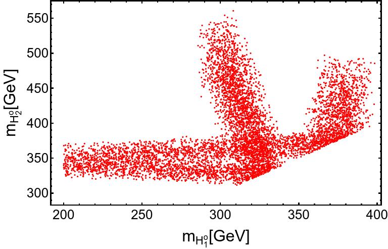
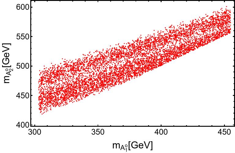
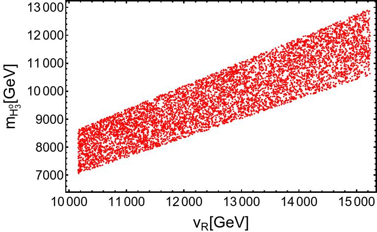
Figure 11: Correlations between the non SM scalar masses (top plots). Correlation between the mass of the CP even neutral scalar $H_{3}^{0}$ and the scale $v_{R}$ of breaking of the left-right symmetry.

VII Higgs diphoton decay rate

The decay rate for the $h\rightarrow\gamma\gamma$ process takes the form:

$$\Gamma(h\rightarrow\gamma\gamma)=\dfrac{\alpha_{em}^{2}m_{h}^{3}}{256\pi^{3}v^{2}}\left|\sum_{f}a_{hff}N_{C}Q_{f}^{2}F_{1/2}(\rho_{f})+a_{hWW}F_{1}(\rho_{W})+\sum_{k=1,2}\frac{C_{hH_{k}^{\pm}H_{k}^{\mp}}v}{2m_{H_{k}^{\pm}}^{2}}F_{0}(\rho_{H_{k}^{\pm}})\right|^{2},$$ (152)

where $\rho_{i}$ are the mass ratios $\rho_{i}=\frac{m_{h}^{2}}{4M_{i}^{2}}$ with $M_{i}=m_{f},M_{W}$; $\alpha_{em}$ is the fine structure constant; $N_{C}$ is the color factor ($N_{C}=1$ for leptons and $N_{C}=3$ for quarks) and $Q_{f}$ is the electric charge of the fermion in the loop. From the fermion-loop contributions we only consider the dominant top quark term. Furthermore, $C_{hH_{k}^{\pm}H_{k}^{\mp}}$ is the trilinear coupling between the SM-like Higgs and a pair of charged Higges, whereas $a_{htt}$ and $a_{hWW}$ are the deviation factors from the SM Higgs-top quark coupling and the SM Higgs-W gauge boson coupling, respectively (in the SM these factors are unity). Such deviation factors are close to unity in our model, which is a consequence of the numerical analysis of its scalar, Yukawa and gauge sectors.

Furthermore, $F_{1/2}(z)$ and $F_{1}(z)$ are the dimensionless loop factors for spin-$1/2$ and spin-$1$ particles running in the internal lines of the loops. They are given by:

$$F_{1/2}(z) =2(z+(z-1)f(z))z^{-2},$$ (153)

$$F_{1}(z) =-2(2z^{2}+3z+3(2z-1)f(z))z^{-2},$$ (154)

$$F_{0}(z) =-(z-f(z))z^{-2},$$ (155)

with

$$f(z)=\left\{\begin{array}[]{lcc}\arcsin^{2}\sqrt{2}&\text{for}&z\leq 1\\ &&\\ -\frac{1}{4}\left(\ln\left(\frac{1+\sqrt{1-z^{-1}}}{1-\sqrt{1-z^{-1}}-i\pi}\right)^{2}\right)&\text{for}&z>1\\ &&\end{array}\right.$$ (156)

In order to study the implications of our model in the decay of the $126$ GeV Higgs into a photon pair, one introduces the Higgs diphoton signal strength $R_{\gamma\gamma}$, which is defined as:

$$R_{\gamma\gamma}=\frac{\sigma(pp\rightarrow h)\Gamma(h\rightarrow\gamma\gamma)}{\sigma(pp\rightarrow h)_{SM}\Gamma(h\rightarrow\gamma\gamma)_{SM}}\simeq a_{htt}^{2}\frac{\Gamma(h\rightarrow\gamma\gamma)}{\Gamma(h\rightarrow\gamma\gamma)_{SM}}.$$ (157)

That Higgs diphoton signal strength, normalizes the $\gamma\gamma$ signal predicted by our model in relation to the one given by the SM. Here we have used the fact that in our model, single Higgs production is also dominated by gluon fusion as in the Standard Model.

The ratio $R_{\gamma\gamma}$ has been measured by CMS and ATLAS collaborations with the best fit signals Sirunyan:2018ouh ; Aad:2019mbh :

$$R_{\gamma\gamma}^{CMS}=1.18_{-0.14}^{+0.17}\quad\text{and}\quad R_{\gamma\gamma}^{ATLAS}=0.96\pm 0.14.$$ (158)

The correlation of the Higgs diphoton signal strength with the charged scalar mass $m_{H_{1}^{\pm}}$ is shown in Figure 12, which indicates that our model successfully accommodates the current Higgs diphoton decay rate constraints. Furthermore, as indicated by Figure 12, our model favours a Higgs diphoton decay rate lower than the SM expectation but inside the $3\sigma$ experimentally allowed range.

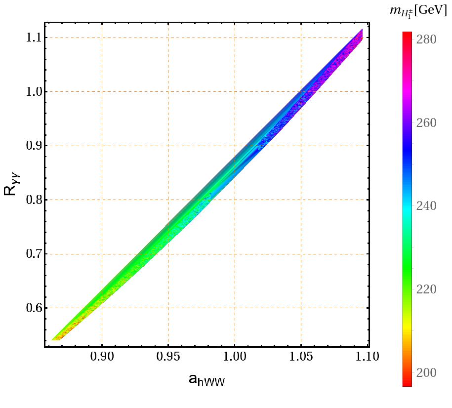
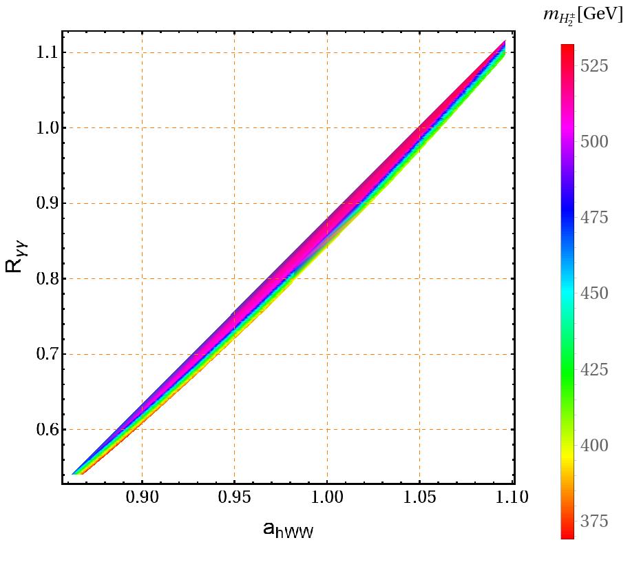
Figure 12: Correlation of the Higgs diphoton signal strength with the $a_{hWW}$ deviation factor from the SM Higgs-W gauge boson coupling.

VIII Muon and electron anomalous magnetic moments

In this section we will analyze the implications of our model in the muon and electron anomalous magnetic moments. The muon and electron anomalous magnetic moments receive contributions arising from vertex diagrams involving the exchange of neutral scalars and charged leptons running in the internal lines of the loop. The Feynman diagramas corresponding to these contributions are shown in Figure 13.

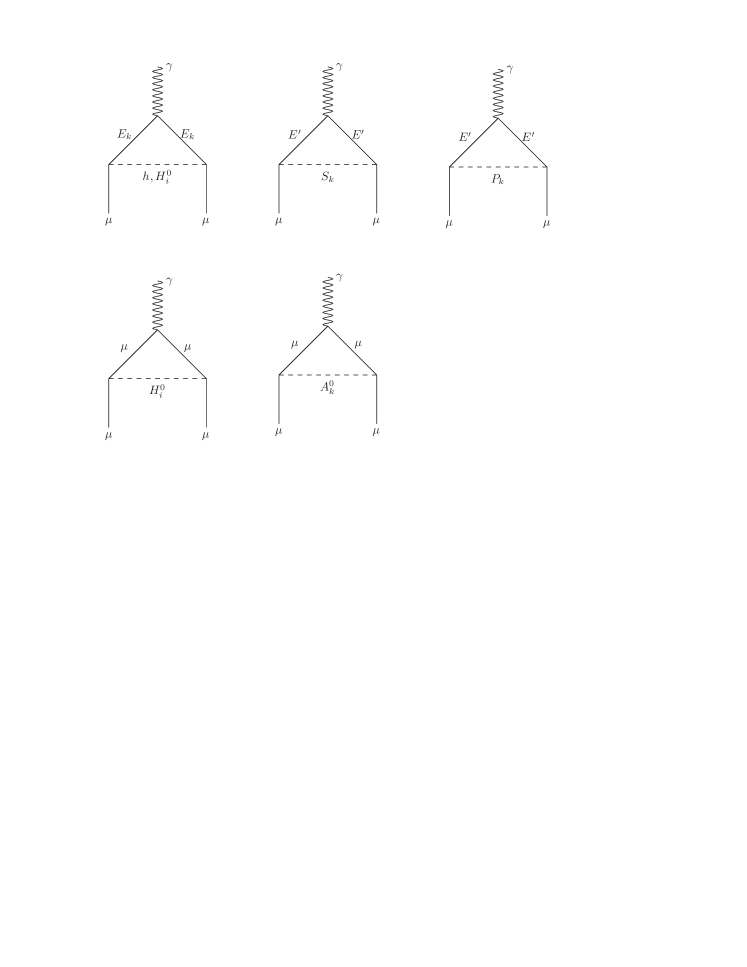
Figure 13: One-loop Feynman diagrams contributing to the muon and electron anomalous magnetic moments. Here $i=1,2,3$, $k=1,2$.

Then, in our model the contributions to the muon and electron anomalous magnetic moments take the form:

$$\Delta a_{\mu} = \mathop{\displaystyle\sum}\limits_{k=1}^{2}\frac{\mathop{\mathrm{R}e}\left(\beta_{2k}\gamma_{k2}^{\ast}\right)m_{\mu}^{2}}{8\pi^{2}}\left(R_{CP-\text{even}}^{T}\right)_{21}\left(R_{CP-\text{even}}^{T}\right)_{41}I_{S}^{\left(\mu\right)}\left(m_{E_{k}},m_{h^{0}}\right)$$

$$+\mathop{\displaystyle\sum}\limits_{k=1}^{2}\frac{\mathop{\mathrm{R}e}\left(\beta_{2k}\gamma_{k2}^{\ast}\right)m_{\mu}^{2}}{8\pi^{2}}\mathop{\displaystyle\sum}\limits_{i=1}^{3}\left(R_{CP-\text{even}}^{T}\right)_{2,i+1}\left(R_{CP-\text{even}}^{T}\right)_{4,i+1}I_{S}^{\left(\mu\right)}\left(m_{E_{k}},m_{H_{i}^{0}}\right)$$

$$+\frac{m_{\mu}^{2}\mathop{\mathrm{R}e}\left(\kappa_{2}\vartheta_{2}^{\ast}\right)}{8\pi^{2}}\left[I_{S}^{\left(\mu\right)}\left(m_{E^{\prime}},m_{S_{1}}\right)-I_{P}^{\left(\mu\right)}\left(m_{E^{\prime}},m_{P_{1}}\right)-I_{S}^{\left(\mu\right)}\left(m_{E^{\prime}},m_{S_{2}}\right)+I_{P}^{\left(\mu\right)}\left(m_{E^{\prime}},m_{P_{2}}\right)\right]\sin\theta\cos\theta$$

$$+\frac{\left|y_{22}^{\left(L\right)}\right|^{2}m_{\mu}^{2}}{8\pi^{2}}\left[\mathop{\displaystyle\sum}\limits_{i=1}^{3}\left|\left(R_{CP-\text{even}}^{T}\right)_{3,i+1}\right|^{2}I_{S}^{\left(\mu\right)}\left(m_{\mu},m_{H_{i}^{0}}\right)+\mathop{\displaystyle\sum}\limits_{i=1}^{2}\left|\left(R_{CP-\text{odd}}^{T}\right)_{4,i+2}\right|^{2}I_{P}^{\left(\mu\right)}\left(m_{\mu},m_{A_{i}^{0}}\right)\right]$$

$$\Delta a_{e} = \mathop{\displaystyle\sum}\limits_{k=1}^{2}\frac{\mathop{\mathrm{R}e}\left(\beta_{1k}\gamma_{k1}^{\ast}\right)m_{e}^{2}}{8\pi^{2}}\left(R_{CP-\text{even}}^{T}\right)_{21}\left(R_{CP-\text{even}}^{T}\right)_{41}I_{S}^{\left(e\right)}\left(m_{E_{k}},m_{h^{0}}\right)$$

$$+\mathop{\displaystyle\sum}\limits_{k=1}^{2}\frac{\mathop{\mathrm{R}e}\left(\beta_{1k}\gamma_{k1}^{\ast}\right)m_{e}^{2}}{8\pi^{2}}\mathop{\displaystyle\sum}\limits_{i=1}^{3}\left(R_{CP-\text{even}}^{T}\right)_{2,i+1}\left(R_{CP-\text{even}}^{T}\right)_{4,i+1}I_{S}^{\left(e\right)}\left(m_{E_{k}},m_{H_{i}^{0}}\right)$$

$$+\frac{m_{e}^{2}\mathop{\mathrm{R}e}\left(\kappa_{1}\vartheta_{1}^{\ast}\right)}{8\pi^{2}}\left[I_{S}^{\left(e\right)}\left(m_{E^{\prime}},m_{S_{1}}\right)-I_{P}^{\left(e\right)}\left(m_{E^{\prime}},m_{P_{1}}\right)-I_{S}^{\left(e\right)}\left(m_{E^{\prime}},m_{S_{2}}\right)+I_{P}^{\left(e\right)}\left(m_{E^{\prime}},m_{P_{2}}\right)\right]\sin\theta\cos\theta$$

$$+\frac{\left|y_{11}^{\left(L\right)}\right|^{2}m_{e}^{2}}{8\pi^{2}}\left[\mathop{\displaystyle\sum}\limits_{i=1}^{3}\left|\left(R_{CP-\text{even}}^{T}\right)_{3,i+1}\right|^{2}I_{S}^{\left(\mu\right)}\left(m_{e},m_{H_{i}^{0}}\right)+\mathop{\displaystyle\sum}\limits_{i=1}^{2}\left|\left(R_{CP-\text{odd}}^{T}\right)_{4,i+2}\right|^{2}I_{P}^{\left(\mu\right)}\left(m_{e},m_{A_{i}^{0}}\right)\right]$$

where $\theta=\theta_{S}=-\theta_{P}$, being $\theta_{S}$ and $\theta_{P}$ the $\mathop{\mathrm{R}e}\phi_{L}^{0}-\mathop{\mathrm{R}e}\phi_{R}^{0}$ and $\mathop{\mathrm{I}m}\phi_{L}^{0}-\mathop{\mathrm{I}m}\phi_{R}^{0}$ mixing angles, respectively. Furthermore, the loop $I_{S\left(P\right)}\left(m_{E},m\right)$ has the form Diaz:2002uk ; Jegerlehner:2009ry ; Kelso:2014qka ; Lindner:2016bgg ; Kowalska:2017iqv :

$$I_{S\left(P\right)}^{\left(e,\mu\right)}\left(m_{E},m_{S}\right)=\int_{0}^{1}\frac{x^{2}\left(1-x\pm\frac{m_{E}}{m_{e,\mu}}\right)}{m_{\mu}^{2}x^{2}+\left(m_{E}^{2}-m_{e,\mu}^{2}\right)x+m_{S,P}^{2}\left(1-x\right)}dx$$ (160)

and the dimensionless parameters $\beta_{1k}$, $\beta_{2k}$, $\gamma_{k1}$, $\gamma_{k2}$, $\kappa_{1}$, $\kappa_{2}$, $\vartheta_{1}$, $\vartheta_{2}$ are given by:

$$\beta_{1k} = \mathop{\displaystyle\sum}\limits_{i=1}^{3}x_{ik}^{\left(E\right)}\left(V_{lL}^{\dagger}\right)_{1i},\hskip 19.91684pt\hskip 19.91684pt\gamma_{k1}=\mathop{\displaystyle\sum}\limits_{j=1}^{3}z_{kj}^{\left(E\right)}\left(V_{lR}\right)_{j1},$$ (161)

$$\beta_{2k} = \mathop{\displaystyle\sum}\limits_{i=1}^{3}x_{ik}^{\left(E\right)}\left(V_{lL}^{\dagger}\right)_{2i},\hskip 19.91684pt\hskip 19.91684pt\gamma_{k2}=\mathop{\displaystyle\sum}\limits_{j=1}^{3}z_{kj}^{\left(E\right)}\left(V_{lR}\right)_{j2},$$ (162)

$$\kappa_{1} = \mathop{\displaystyle\sum}\limits_{i=1}^{3}w_{i}^{\left(E^{\prime}\right)}\left(V_{lL}^{\dagger}\right)_{1i},\hskip 19.91684pt\hskip 19.91684pt\vartheta_{1}=\mathop{\displaystyle\sum}\limits_{j=1}^{3}r_{j}^{\left(E^{\prime}\right)}\left(V_{lR}\right)_{j1},$$ (163)

$$\kappa_{2} = \mathop{\displaystyle\sum}\limits_{i=1}^{3}w_{i}^{\left(E^{\prime}\right)}\left(V_{lL}^{\dagger}\right)_{2i},\hskip 19.91684pt\hskip 19.91684pt\vartheta_{2}=\mathop{\displaystyle\sum}\limits_{j=1}^{3}r_{j}^{\left(E^{\prime}\right)}\left(V_{lR}\right)_{j2},$$ (164)

where $V_{lL}$ and $V_{lR}$ are the rotation matrices that diagonalize $\widetilde{M}_{E}$ according to the relation:

$$V_{lL}^{\dagger}\widetilde{M}_{E}V_{lR}=diag\left(m_{e},m_{\mu},m_{\tau}\right)$$ (165)

Considering that the muon and electron anomalous magnetic moments are constrained to be in the ranges Abi:2021gix ; Morel:2020dww :

$$\left(\Delta a_{\mu}\right)_{\exp} = \left(2.51\pm 0.59\right)\times 10^{-9}$$

$$(\Delta a_{e})_{\text{exp}} = (4.8\pm 3.0)\times 10^{-13}.$$ (166)

We plot in Figure 14 the correlations of the muon and electron anomalous magnetic moments with the masses $m_{A^{0}_{1}}$ and $m_{A^{0}_{2}}$ of the CP odd neutral scalar (top plots) as well as the correlation between the electron and muon anomalous magnetic moments (bottom plot). We find that our model can successfully accommodates the experimental values of the muon and electron anomalous magnetic moments.

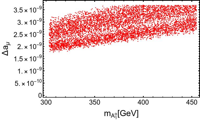
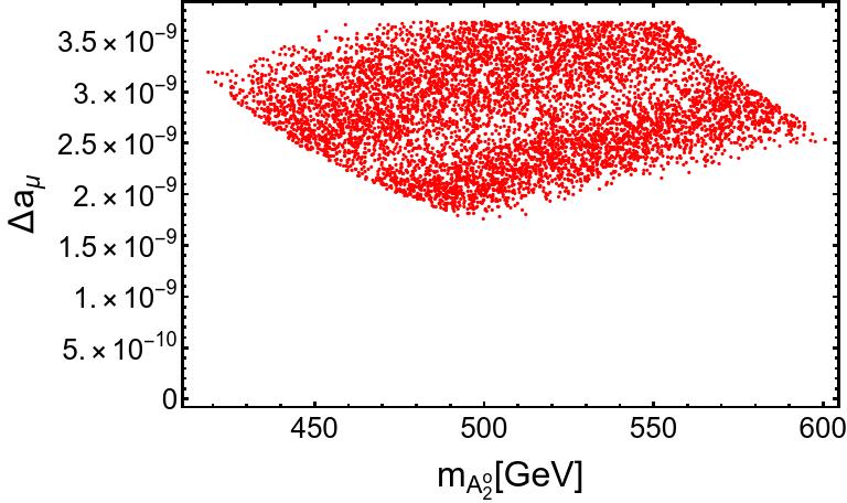
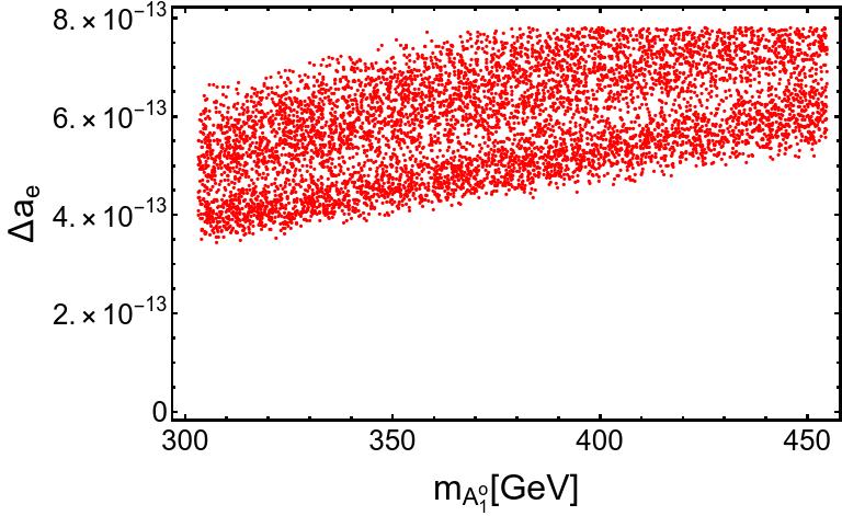
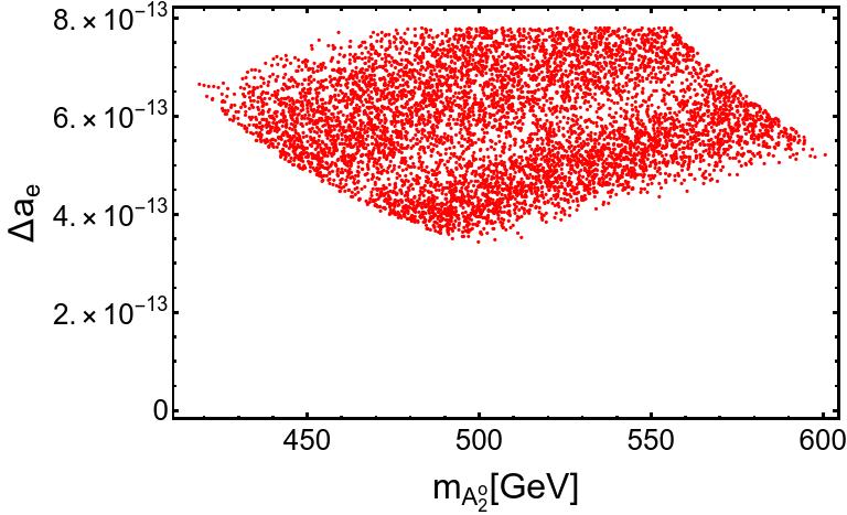
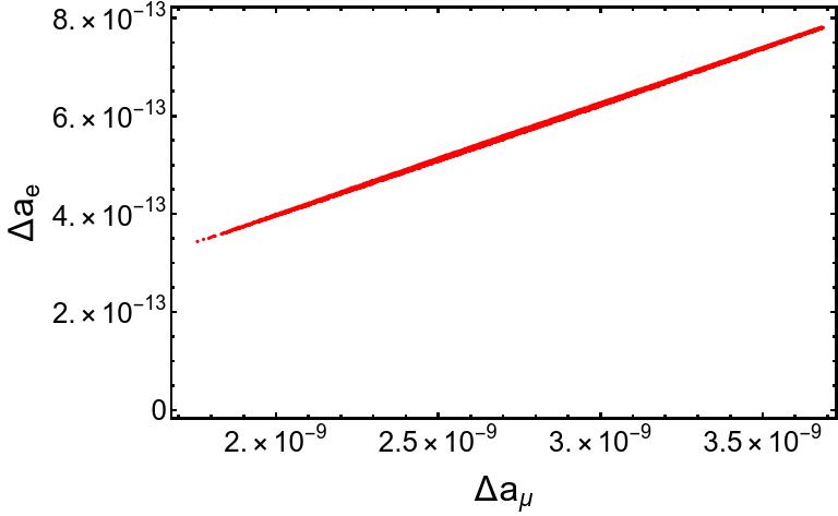
Figure 14: Correlations of the muon and electron anomalous magnetic moments with the masses $m_{A^{0}_{1}}$ and $m_{A^{0}_{2}}$ of the CP odd neutral scalars (top plots). Correlation between the electron and muon anomalous magnetic moments (bottom plot).

IX Heavy scalar production at the LHC

In this section we discuss the singly heavy scalar $H_{1}^{0}$ production at a proton-proton collider. Such production mechanism at the LHC is dominated by the gluon fusion mechanism, which is a one-loop process mediated by the top quark. Thus, the total $H_{1}^{0}$ production cross section in proton-proton collisions with center of mass energy $\sqrt{S}$ takes the form:

$$\sigma_{pp\rightarrow gg\rightarrow H_{1}^{0}}\left(S\right)=\frac{\alpha_{S}^{2}a_{H_{1}^{0}t\bar{t}}^{2}m_{H_{1}^{0}}^{2}}{64\pi v^{2}S}\left[I\left(\frac{m_{H_{1}^{0}}^{2}}{m_{t}^{2}}\right)\right]^{2}\int_{\ln\sqrt{\frac{m_{H_{1}^{0}}^{2}}{S}}}^{-\ln\sqrt{\frac{m_{H_{1}^{0}}^{2}}{S}}}f_{p/g}\left(\sqrt{\frac{m_{H_{1}^{0}}^{2}}{S}}e^{y},\mu^{2}\right)f_{p/g}\left(\sqrt{\frac{m_{H_{1}^{0}}^{2}}{S}}e^{-y},\mu^{2}\right)dy,$$ (167)

where $f_{p/g}\left(x_{1},\mu^{2}\right)$ and $f_{p/g}\left(x_{2},\mu^{2}\right)$ are the distributions of gluons in the proton which carry momentum fractions $x_{1}$ and $x_{2}$ of the proton, respectively. Furthermore $\mu=m_{H_{1}}$ is the factorization scale, whereas $I(z)$ has the form:

$$I(z)=\int_{0}^{1}dx\int_{0}^{1-x}dy\frac{1-4xy}{1-zxy}.$$ (168)

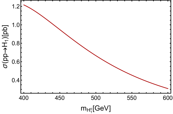
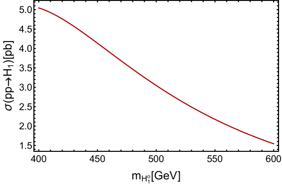
Figure 15: Total cross section for the $H_{1}^{0}$ production via gluon fusion mechanism at the LHC for $\sqrt{s}=14$ TeV (left-panel) and $\sqrt{S}=28$ (right-panel) TeV as a function of the heavy scalar mass $m_{H_{1}^{0}}$.

Figure 15 shows the $H_{1}^{0}$ total production cross section at the LHC via gluon fusion mechanism for $\sqrt{S}=14$ TeV (left-plot) and $\sqrt{S}=28$ TeV (right-plot), as a function of the scalar mass $m_{H_{1}^{0}}$, which is taken to range from $400$ GeV up to $600$ GeV. Furthermore, the coupling $a_{H_{1}^{0}t\bar{t}}$ of the heavy scalar $H_{1}^{0}$ with the top-antitop quark pair has been set to be equal to $0.4$, which is consistent with our numerical analysis of the scalar potential. In the aforementioned region of masses for the heavy $H_{1}$ scalar, we find that the total production cross section ranges from $1.2$ pb up to $0.3$ pb. However, at the proposed energy upgrade of the LHC with $\sqrt{S}=28$ TeV, the total cross section for the $H_{1}^{0}$ is enhanced reaching values between $5$ pb and $1.5$ pb in the aforementioned mass range as indicated in the right panel of Figure 15. The heavy neutral $H_{1}^{0}$ scalar, after being produced, will have dominant decay modes into top-antitop quark pairs, SM Higgs boson pairs as well as into a pair of SM gauge bosons, thus implying that the observation of an excess of events in the multileptons or multijet final states over the SM background can be a smoking gun signature of this model, whose observation will be crucial to assess its viability.

X $Z^{\prime}$ gauge boson production at the LHC

In this section we discuss the single heavy $Z^{\prime}$ gauge boson via Drell-Yan mechanism at proton-proton collider. We consider the dominant contributions due to the parton distribution functions of the light up, down and strange quarks, so that the total cross section for the production of a $Z^{\prime}$ via quark antiquark annihilation in proton-proton collisions with center of mass energy $\sqrt{S}$ takes the form:

$$\sigma_{pp\rightarrow Z^{\prime}}^{\left(DrellYan\right)}(S)=\frac{g_{R}^{2}\pi}{24S}\int_{\ln\sqrt{\frac{m_{Z^{\prime}}^{2}}{S}}}^{-\ln\sqrt{\frac{m_{Z^{\prime}}^{2}}{S}}}\mathop{\displaystyle\sum}\limits_{q=u,d,s}f_{p/q}\left(\sqrt{\frac{m_{Z^{\prime}}^{2}}{S}}e^{y},\mu^{2}\right)f_{p/\overline{q}}\left(\sqrt{\frac{m_{Z^{\prime}}^{2}}{S}}e^{-y},\mu^{2}\right)dy$$ (169)

where $f_{p/u}\left(x_{1},\mu^{2}\right)$ ($f_{p/\overline{u}}\left(x_{2},\mu^{2}\right)$), $f_{p/d}\left(x_{1},\mu^{2}\right)$ ($f_{p/\overline{d}}\left(x_{2},\mu^{2}\right)$) and $f_{p/s}\left(x_{1},\mu^{2}\right)$ ($f_{p/\overline{s}}\left(x_{2},\mu^{2}\right)$) are the distributions of the light up, down and strange quarks (antiquarks), respectively, in the proton which carry momentum fractions $x_{1}$ ($x_{2}$) of the proton. The factorization scale is taken to be $\mu=m_{Z^{\prime}}$.

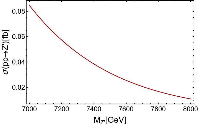
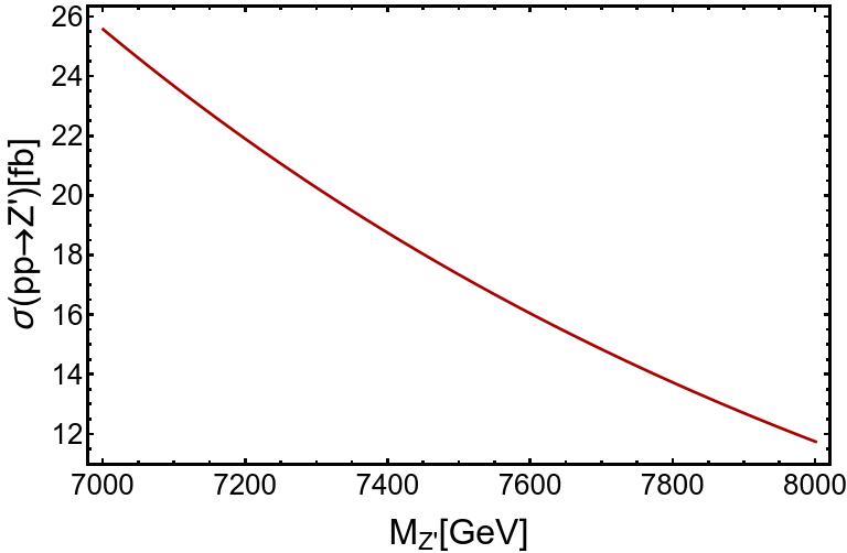
Figure 16: Total cross section for the $Z^{\prime}$ production via Drell-Yan mechanism at a proton-proton collider for $\sqrt{S}=14$ TeV (left-panel) and $\sqrt{S}=28$ (right-panel) TeV as a function of the $Z^{\prime}$ mass.

Fig. 16 displays the $Z^{\prime}$ total production cross section at the LHC via the Drell-Yan mechanism for $\sqrt{S}=14$ TeV (left panel) and $\sqrt{S}=28$ TeV (right panel) as a function of the $Z^{\prime}$ mass $M_{Z^{\prime}}$ in the range from $7$ TeV up to $8$ TeV. We consider $Z^{\prime}$ gauge boson masses larger than $7$ TeV and we set $g_{R}=1$, which is consistent with the constraint $\frac{M_{Z^{\prime}}}{g_{R}}>7$ TeV arising from LEP I and II measurements of $e^{+}e^{-}\rightarrow l^{+}l^{-}$ LEP:2004xhf ; Carena:2004xs ; Das:2021esm as well as with the ones resulting from LHC searches ATLAS:2019erb ; CMS:2021ctt . Limits on the ratio $\frac{M_{Z^{\prime}}}{g_{R}}$ are derived in Ref. Das:2021esm , both for LEP II as well as for different values of the center of mass energy $\sqrt{s}$ of the future International Linear (ILC) $e^{+}e^{-}$ Collider. In this work we use the LEP II bound $\frac{M_{Z^{\prime}}}{g_{R}}>7$ TeV, since the other bounds correspond to future projective limits related to experiments which have not been started yet. With respect to the bounds of the $W^{\prime}$ gauge boson mass, CMS and ATLAS experiments at CERN have found that the $W^{\prime}$ gauge boson should be heavier than $6$ TeV CMS:2021qef and $5$ TeV ATLAS:2018dcj , respectively.

For this region of $Z^{\prime}$ masses we find that the total production cross section ranges from $0.85$ fb up to $0.01$ fb. The heavy neutral $Z^{\prime}$ gauge boson, after being produced, will subsequently decay into the pair of the SM fermion-antifermion pairs, thus implying that the observation of an excess of events in the dileptons or dijet final states over the SM background can be a signal of support of this model at the LHC. On the other hand, at the proposed energy upgrade of the LHC at 28 TeV center of mass energy, the total cross section for the Drell-Yan production of a heavy $Z^{\prime}$ neutral gauge boson gets significantly enhanced reaching values ranging from $26$ fb up to $12$ fb, as indicated in the right panel of Fig. 16.

XI Meson oscillations

In this section, we discuss the implications of our model in the Flavour Changing Neutral Current (FCNC) interactions in the down type quark sector. The FCNC Yukawa interactions in the down type quark sector give rise to meson oscillations. The following effective Hamiltonians describe $K^{0}-\bar{K}^{0}$, $B_{d}^{0}-\bar{B}_{d}^{0}$ and $B_{s}^{0}-\bar{B}_{s}^{0}$ mixings:

$$\mathcal{H}_{eff}^{\left(K^{0}-\bar{K}^{0}\right)}\mathcal{=}\frac{G_{F}^{2}m_{W}^{2}}{16\pi^{2}}\sum_{i=1}^{3}C_{i}^{\left(K^{0}-\bar{K}^{0}\right)}\left(\mu\right)O_{i}^{\left(K^{0}-\bar{K}^{0}\right)}\left(\mu\right),$$ (170)

$$\mathcal{H}_{eff}^{\left(B_{d}^{0}-\bar{B}_{d}^{0}\right)}\mathcal{=}\frac{G_{F}^{2}m_{W}^{2}}{16\pi^{2}}\sum_{i=1}^{3}C_{i}^{\left(B_{d}^{0}-\bar{B}_{d}^{0}\right)}\left(\mu\right)O_{i}^{\left(B_{d}^{0}-\bar{B}_{d}^{0}\right)}\left(\mu\right),$$ (171)

$$\mathcal{H}_{eff}^{\left(B_{s}^{0}-\bar{B}_{s}^{0}\right)}\mathcal{=}\frac{G_{F}^{2}m_{W}^{2}}{16\pi^{2}}\sum_{i=1}^{3}C_{i}^{\left(B_{s}^{0}-\bar{B}_{s}^{0}\right)}\left(\mu\right)O_{i}^{\left(B_{s}^{0}-\bar{B}_{s}^{0}\right)}\left(\mu\right),$$ (172)

In our analysis of meson oscillations we follow the approach of Dedes:2002er ; Aranda:2012bv . The $K^{0}-\bar{K}^{0}$, $B_{d}^{0}-\bar{B}_{d}^{0}$ and $B_{s}^{0}-\bar{B}_{s}^{0}$ meson mixings receive tree level contributions corresponding to the exchange of neutral CP even and CP odd scalars, thus giving rise to the following operators:

$$O_{1}^{\left(K^{0}-\bar{K}^{0}\right)} = \left(\overline{s}P_{L}d\right)\left(\overline{s}P_{L}d\right),\hskip 28.45274ptO_{2}^{\left(K^{0}-\bar{K}^{0}\right)}=\left(\overline{s}P_{R}d\right)\left(\overline{s}P_{R}d\right),\hskip 28.45274ptO_{3}^{\left(K^{0}-\bar{K}^{0}\right)}=\left(\overline{s}P_{L}d\right)\left(\overline{s}P_{R}d\right),$$ (173)

$$O_{1}^{\left(B_{d}^{0}-\bar{B}_{d}^{0}\right)} = \left(\overline{d}P_{L}b\right)\left(\overline{d}P_{L}b\right),\hskip 28.45274ptO_{2}^{\left(B_{d}^{0}-\bar{B}_{d}^{0}\right)}=\left(\overline{d}P_{R}b\right)\left(\overline{d}P_{R}b\right),\hskip 28.45274ptO_{3}^{\left(B_{d}^{0}-\bar{B}_{d}^{0}\right)}=\left(\overline{d}P_{L}b\right)\left(\overline{d}P_{R}b\right),\hskip 19.91684pt$$ (174)

$$O_{1}^{\left(B_{s}^{0}-\bar{B}_{s}^{0}\right)} = \left(\overline{s}P_{L}b\right)\left(\overline{s}P_{L}b\right),\hskip 28.45274ptO_{2}^{\left(B_{s}^{0}-\bar{B}_{s}^{0}\right)}=\left(\overline{s}P_{R}b\right)\left(\overline{s}P_{R}b\right),\hskip 28.45274ptO_{3}^{\left(B_{s}^{0}-\bar{B}_{s}^{0}\right)}=\left(\overline{s}P_{L}b\right)\left(\overline{s}P_{R}b\right),$$ (175)

where the corresponding Wilson coefficients are given by:

$$C_{1}^{\left(K^{0}-\bar{K}^{0}\right)} = \frac{16\pi^{2}}{G_{F}^{2}m_{W}^{2}}\widetilde{C}_{1}^{\left(K^{0}-\bar{K}^{0}\right)},\hskip 19.91684pt\hskip 19.91684pt\widetilde{C}_{1}^{\left(K^{0}-\bar{K}^{0}\right)}=\frac{y_{h\overline{s}_{R}d_{L}}^{2}}{m_{h}^{2}}+\sum_{i=1}^{3}\frac{y_{H_{i}^{0}\overline{s}_{R}d_{L}}^{2}}{m_{H_{i}^{0}}^{2}}-\sum_{i=1}^{2}\frac{y_{A_{i}^{0}\overline{s}_{R}d_{L}}^{2}}{m_{A_{i}^{0}}^{2}},$$ (176)

$$C_{2}^{\left(K^{0}-\bar{K}^{0}\right)} = \frac{16\pi^{2}}{G_{F}^{2}m_{W}^{2}}\widetilde{C}_{2}^{\left(K^{0}-\bar{K}^{0}\right)},\hskip 19.91684pt\hskip 19.91684pt\widetilde{C}_{2}^{\left(K^{0}-\bar{K}^{0}\right)}=\frac{y_{h\overline{s}_{L}d_{R}}^{2}}{m_{h}^{2}}+\sum_{i=1}^{3}\frac{y_{H_{i}^{0}\overline{s}_{L}d_{R}}^{2}}{m_{H_{i}^{0}}^{2}}-\sum_{i=1}^{2}\frac{y_{A_{i}^{0}\overline{s}_{L}d_{R}}^{2}}{m_{A_{i}^{0}}^{2}},$$ (177)

$$C_{3}^{\left(K^{0}-\bar{K}^{0}\right)} = \frac{16\pi^{2}}{G_{F}^{2}m_{W}^{2}}\widetilde{C}_{3}^{\left(K^{0}-\bar{K}^{0}\right)},\hskip 8.5359pt\widetilde{C}_{3}^{\left(K^{0}-\bar{K}^{0}\right)}=\frac{y_{h\overline{s}_{R}d_{L}}y_{h\overline{s}_{L}d_{R}}}{m_{h}^{2}}+\sum_{i=1}^{3}\frac{y_{H_{i}^{0}\overline{s}_{R}d_{L}}y_{H_{i}^{0}\overline{s}_{L}d_{R}}}{m_{H_{i}^{0}}^{2}}-\sum_{i=1}^{2}\frac{y_{A_{i}^{0}\overline{s}_{R}d_{L}}y_{A_{i}^{0}\overline{s}_{L}d_{R}}}{m_{A_{i}^{0}}^{2}},$$ (178)

$$C_{1}^{\left(B_{d}^{0}-\bar{B}_{d}^{0}\right)} = \frac{16\pi^{2}}{G_{F}^{2}m_{W}^{2}}\widetilde{C}_{1}^{\left(B_{d}^{0}-\bar{B}_{d}^{0}\right)},\hskip 19.91684pt\hskip 19.91684pt\widetilde{C}_{1}^{\left(B_{d}^{0}-\bar{B}_{d}^{0}\right)}=\frac{y_{h\overline{d}_{R}b_{L}}^{2}}{m_{h}^{2}}+\sum_{i=1}^{3}\frac{y_{H_{i}^{0}\overline{d}_{R}b_{L}}^{2}}{m_{H_{i}^{0}}^{2}}-\sum_{i=1}^{2}\frac{y_{A_{i}^{0}\overline{d}_{R}b_{L}}^{2}}{m_{A_{i}^{0}}^{2}},$$ (179)

$$C_{2}^{\left(B_{d}^{0}-\bar{B}_{d}^{0}\right)} = \frac{16\pi^{2}}{G_{F}^{2}m_{W}^{2}}\widetilde{C}_{2}^{\left(B_{d}^{0}-\bar{B}_{d}^{0}\right)},\hskip 19.91684pt\hskip 19.91684pt\widetilde{C}_{2}^{\left(B_{d}^{0}-\bar{B}_{d}^{0}\right)}=\frac{y_{h\overline{d}_{L}b_{R}}^{2}}{m_{h}^{2}}+\sum_{i=1}^{3}\frac{y_{H_{i}^{0}\overline{d}_{L}b_{R}}^{2}}{m_{H_{i}^{0}}^{2}}-\sum_{i=1}^{2}\frac{y_{A_{i}^{0}\overline{d}_{L}b_{R}}^{2}}{m_{A_{i}^{0}}^{2}},$$ (180)

$$C_{3}^{\left(B_{d}^{0}-\bar{B}_{d}^{0}\right)} = \frac{16\pi^{2}}{G_{F}^{2}m_{W}^{2}}\widetilde{C}_{3}^{\left(B_{d}^{0}-\bar{B}_{d}^{0}\right)},\hskip 8.5359pt\widetilde{C}_{3}^{\left(B_{d}^{0}-\bar{B}_{d}^{0}\right)}=\frac{y_{h\overline{d}_{R}b_{L}}y_{h\overline{d}_{L}b_{R}}}{m_{h}^{2}}+\sum_{i=1}^{3}\frac{y_{H_{i}^{0}\overline{d}_{R}b_{L}}y_{H_{i}^{0}\overline{d}_{L}b_{R}}}{m_{H_{i}^{0}}^{2}}-\sum_{i=1}^{2}\frac{y_{A_{i}^{0}\overline{d}_{R}b_{L}}y_{A_{i}^{0}\overline{d}_{L}b_{R}}}{m_{A_{i}^{0}}^{2}},$$ (181)

$$C_{1}^{\left(B_{s}^{0}-\bar{B}_{s}^{0}\right)} = \frac{16\pi^{2}}{G_{F}^{2}m_{W}^{2}}\widetilde{C}_{1}^{\left(B_{s}^{0}-\bar{B}_{s}^{0}\right)},\hskip 19.91684pt\hskip 19.91684pt\widetilde{C}_{1}^{\left(B_{s}^{0}-\bar{B}_{s}^{0}\right)}=\frac{y_{h\overline{s}_{R}b_{L}}^{2}}{m_{h}^{2}}+\sum_{i=1}^{3}\frac{y_{H_{i}^{0}\overline{s}_{R}b_{L}}^{2}}{m_{H_{i}^{0}}^{2}}-\sum_{i=1}^{2}\frac{y_{A_{i}^{0}\overline{s}_{R}b_{L}}^{2}}{m_{A_{i}^{0}}^{2}},$$ (182)

$$C_{2}^{\left(B_{s}^{0}-\bar{B}_{s}^{0}\right)} = \frac{16\pi^{2}}{G_{F}^{2}m_{W}^{2}}\widetilde{C}_{2}^{\left(B_{s}^{0}-\bar{B}_{s}^{0}\right)},\hskip 19.91684pt\hskip 19.91684pt\widetilde{C}_{2}^{\left(B_{s}^{0}-\bar{B}_{s}^{0}\right)}=\frac{y_{h\overline{s}_{L}b_{R}}^{2}}{m_{h}^{2}}+\sum_{i=1}^{3}\frac{y_{H_{i}^{0}\overline{s}_{L}b_{R}}^{2}}{m_{H_{i}^{0}}^{2}}-\sum_{i=1}^{2}\frac{y_{A_{i}^{0}\overline{s}_{L}b_{R}}^{2}}{m_{A_{i}^{0}}^{2}},$$ (183)

$$C_{3}^{\left(B_{s}^{0}-\bar{B}_{s}^{0}\right)} = \frac{16\pi^{2}}{G_{F}^{2}m_{W}^{2}}\widetilde{C}_{3}^{\left(B_{s}^{0}-\bar{B}_{s}^{0}\right)},\hskip 8.5359pt\widetilde{C}_{3}^{\left(B_{s}^{0}-\bar{B}_{s}^{0}\right)}=\frac{y_{h\overline{s}_{R}b_{L}}y_{h\overline{s}_{L}b_{R}}}{m_{h}^{2}}+\sum_{i=1}^{3}\frac{y_{H_{i}^{0}\overline{s}_{R}b_{L}}y_{H_{i}^{0}\overline{s}_{L}b_{R}}}{m_{H_{i}^{0}}^{2}}-\sum_{i=1}^{2}\frac{y_{A_{i}^{0}\overline{s}_{R}b_{L}}y_{A_{i}^{0}\overline{s}_{L}b_{R}}}{m_{A_{i}^{0}}^{2}},$$ (184)

Furthermore, the $K-\bar{K}$, $B_{d}^{0}-\bar{B}_{d}^{0}$ and $B_{s}^{0}-\bar{B}_{s}^{0}$ mass splittings can be written as:

$$\Delta m_{K}=\left(\Delta m_{K}\right)_{SM}+\Delta m_{K}^{\left(NP\right)},\hskip 28.45274pt\Delta m_{B_{d}}=\left(\Delta m_{B_{d}}\right)_{SM}+\Delta m_{B_{d}}^{\left(NP\right)},\hskip 28.45274pt\Delta m_{B_{s}}=\left(\Delta m_{B_{s}}\right)_{SM}+\Delta m_{B_{s}}^{\left(NP\right)},$$ (185)

where $\left(\Delta m_{K}\right)_{SM}$, $\left(\Delta m_{B_{d}}\right)_{SM}$ and $\left(\Delta m_{B_{s}}\right)_{SM}$ are the SM contributions, whereas $\Delta m_{K}^{\left(NP\right)}$ , $\Delta m_{B_{d}}^{\left(NP\right)}$ and $\left(\Delta m_{B_{s}}\right)_{SM}$ are new physics contributions.

In our model, the new physics contributions to the meson differences are given by:

$$\Delta m_{K}^{\left(NP\right)} = \frac{G_{F}^{2}m_{W}^{2}}{6\pi^{2}}m_{K}f_{K}^{2}\eta_{K}B_{K}\left[P_{2}^{\left(K^{0}-\bar{K}^{0}\right)}C_{3}^{\left(K^{0}-\bar{K}^{0}\right)}+P_{1}^{\left(K^{0}-\bar{K}^{0}\right)}\left(C_{1}^{\left(K^{0}-\bar{K}^{0}\right)}+C_{2}^{\left(K^{0}-\bar{K}^{0}\right)}\right)\right]$$ (186)

$$= \frac{8}{3}m_{K}f_{K}^{2}\eta_{K}B_{K}\left[P_{2}^{\left(K^{0}-\bar{K}^{0}\right)}\widetilde{C}_{3}^{\left(K^{0}-\bar{K}^{0}\right)}+P_{1}^{\left(K^{0}-\bar{K}^{0}\right)}\left(\widetilde{C}_{1}^{\left(K^{0}-\bar{K}^{0}\right)}+\widetilde{C}_{2}^{\left(K^{0}-\bar{K}^{0}\right)}\right)\right]$$

$$\Delta m_{B_{d}}^{\left(NP\right)} = \frac{G_{F}^{2}m_{W}^{2}}{6\pi^{2}}m_{B_{d}}f_{B_{d}}^{2}\eta_{B_{d}}B_{B_{d}}\left[P_{2}^{\left(B_{d}^{0}-\bar{B}_{d}^{0}\right)}C_{3}^{\left(B_{d}^{0}-\bar{B}_{d}^{0}\right)}+P_{1}^{\left(B_{d}^{0}-\bar{B}_{d}^{0}\right)}\left(C_{1}^{\left(B_{d}^{0}-\bar{B}_{d}^{0}\right)}+C_{2}^{\left(B_{d}^{0}-\bar{B}_{d}^{0}\right)}\right)\right]$$ (187)

$$= \frac{8}{3}m_{B_{d}}f_{B_{d}}^{2}\eta_{B_{d}}B_{B_{d}}\left[P_{2}^{\left(B_{d}^{0}-\bar{B}_{d}^{0}\right)}\widetilde{C}_{3}^{\left(B_{d}^{0}-\bar{B}_{d}^{0}\right)}+P_{1}^{\left(B_{d}^{0}-\bar{B}_{d}^{0}\right)}\left(\widetilde{C}_{1}^{\left(B_{d}^{0}-\bar{B}_{d}^{0}\right)}+\widetilde{C}_{2}^{\left(B_{d}^{0}-\bar{B}_{d}^{0}\right)}\right)\right]$$

$$\Delta m_{B_{s}}^{\left(NP\right)} = \frac{G_{F}^{2}m_{W}^{2}}{6\pi^{2}}m_{B_{s}}f_{B_{s}}^{2}\eta_{B_{s}}B_{B_{s}}\left[P_{2}^{\left(B_{s}^{0}-\bar{B}_{s}^{0}\right)}C_{3}^{\left(B_{s}^{0}-\bar{B}_{s}^{0}\right)}+P_{1}^{\left(B_{s}^{0}-\bar{B}_{s}^{0}\right)}\left(C_{1}^{\left(B_{s}^{0}-\bar{B}_{s}^{0}\right)}+C_{2}^{\left(B_{s}^{0}-\bar{B}_{s}^{0}\right)}\right)\right]$$ (188)

$$= \frac{8}{3}m_{B_{s}}f_{B_{s}}^{2}\eta_{B_{s}}B_{B_{s}}\left[P_{2}^{\left(B_{s}^{0}-\bar{B}_{s}^{0}\right)}\widetilde{C}_{3}^{\left(B_{s}^{0}-\bar{B}_{s}^{0}\right)}+P_{1}^{\left(B_{s}^{0}-\bar{B}_{s}^{0}\right)}\left(\widetilde{C}_{1}^{\left(B_{s}^{0}-\bar{B}_{s}^{0}\right)}+\widetilde{C}_{2}^{\left(B_{s}^{0}-\bar{B}_{s}^{0}\right)}\right)\right]$$

Using the following parameters Dedes:2002er ; Aranda:2012bv ; Khalil:2013ixa ; Queiroz:2016gif ; Buras:2016dxz ; Ferreira:2017tvy ; Duy:2020hhk ; Branco:2021vhs ; Zyla:2020zbs :

$$\Delta m_{K} = \left(3.484\pm 0.006\right)\times 10^{-12}MeV,\hskip 42.67912pt\left(\Delta m_{K}\right)_{SM}=3.483\times 10^{-12}MeV$$

$$f_{K} = \left(155.7\pm 0.3\right)MeV,\hskip 42.67912ptB_{K}=0.717\pm 0.024,\hskip 42.67912pt\eta_{K}=0.57,$$

$$P_{1}^{\left(K^{0}-\bar{K}^{0}\right)} = -9.3,\hskip 42.67912ptP_{2}^{\left(K^{0}-\bar{K}^{0}\right)}=30.6,\hskip 42.67912ptm_{K}=\left(497.611\pm 0.013\right)MeV,\hskip 42.67912pt$$ (189)

$$\left(\Delta m_{B_{d}}\right)_{\exp} = \left(3.334\pm 0.013\right)\times 10^{-10}MeV,\hskip 42.67912pt\left(\Delta m_{B_{d}}\right)_{SM}=3.582\times 10^{-10}MeV,$$

$$f_{B_{d}} = \left(190.0\pm 1.3\right)MeV,\hskip 42.67912ptB_{B_{d}}=1.30\pm 0.10,\hskip 42.67912pt\eta_{B_{d}}=0.55,$$

$$P_{1}^{\left(B_{d}^{0}-\bar{B}_{d}^{0}\right)} = -0.52,\hskip 42.67912ptP_{2}^{\left(B_{d}^{0}-\bar{B}_{d}^{0}\right)}=0.88,\hskip 42.67912ptm_{B_{d}}=\left(5279.65\pm 0.12\right)MeV,\hskip 42.67912pt$$ (190)

$$\left(\Delta m_{B_{s}}\right)_{\exp} = \left(1.1683\pm 0.0013\right)\times 10^{-8}MeV,\hskip 42.67912pt\left(\Delta m_{B_{s}}\right)_{SM}=1.21103\times 10^{-8}MeV,$$

$$f_{B_{s}} = \left(230.3\pm 1.3\right)MeV,\hskip 42.67912ptB_{B_{s}}=1.35\pm 0.06,\hskip 42.67912pt\eta_{B_{s}}=0.55,$$

$$P_{1}^{\left(B_{s}^{0}-\bar{B}_{s}^{0}\right)} = -0.52,\hskip 42.67912ptP_{2}^{\left(B_{s}^{0}-\bar{B}_{s}^{0}\right)}=0.88,\hskip 42.67912ptm_{B_{s}}=\left(5366.88\pm 0.14\right)MeV,\hskip 42.67912pt$$ (191)

Figure 17 displays the correlation between the $\Delta m_{B_{d}}$ mass splitting and the heavy CP even scalar mass $m_{H_{1}^{0}}$. In our numerical analysis, for the sake of simplicity, we have set the couplings of the flavor changing neutral Yukawa interactions that produce the $B_{d}^{0}-\bar{B}_{d}^{0}$ oscillations to be equal to $10^{-4}$. Furthermore, we have fixed $m_{H_{3}^{0}}=10$ TeV and we have varied the masses of $H_{1}^{0}$, $H_{2}^{0}$ and $A_{1}^{0}$ in the ranges $200$ GeV$\leqslant m_{H_{1}^{0}}\leqslant$ $400$ GeV, $350$ GeV$\leqslant m_{H_{2}^{0}}\leqslant$ $550$ GeV and $300$ GeV$\leqslant m_{A_{1}^{0}}\leqslant$ $450$ GeV, whereas we have also set $m_{A_{2}^{0}}=m_{A_{1}^{0}}+150GeV$. It is worth mentioning that the above described ranges of scalar masses is consistent with the ones described in the correlation plots of heavy scalar masses shown in Figure 11. As indicated in Figure 17, the experimental constraints arising from $B_{d}^{0}-\bar{B}_{d}^{0}$ meson oscillations are successfully fullfilled for the aforementioned range of parameter space. We have numerically checked that in the above described range of masses, the obtained values for the $\Delta m_{B_{s}}$ and $\Delta m_{K}$ mass splittings are consistent with the experimental data on meson oscillations for flavor violating Yukawa couplings equal to $2.5\times 10^{-4}$ and $10^{-6}$ for the $B_{s}^{0}-\bar{B}_{s}^{0}$ and $K^{0}-\bar{K}^{0}$ mixings, respectively.

Figure 17: Correlation between the $\Delta m_{B_{d}}$ mass splitting and the heavy CP even scalar mass $m_{H_{1}^{0}}$. The couplings of the flavor changing neutral Yukawa interactions have been set to be equal to $10^{-4}$.

XII Conclusions

We have built a renormalizable left-right symmetric theory with additional symmetry $Z_{4}^{\left(1\right)}\times Z_{4}^{\left(2\right)}$ consistent with the observed SM fermion mass hierarchy, the tiny values for the light active neutrino masses, the lepton and baryon asymmetries of the Universe, the constraints arising from meson oscillations, from charged lepton flavor violation, as well as the muon and electron anomalous magnetic moments. As the main appealing feature of the proposed model, the top and exotic fermions get their masses at tree level whereas the masses of the bottom, charm and strange quarks, tau and muon leptons are generated from a tree level Universal Seesaw mechanism thanks to their mixings with charged exotic vector like fermions. The first generation SM charged fermions masses are produced from a radiative seesaw mechanism at one loop level mediated by charged vector like fermions and electrically neutral scalars. The tiny masses of the light active neutrinos arise from an inverse seesaw mechanism at one-loop level. Furthermore, we have also shown that the proposed model successfully accommodates the current Higgs diphoton decay rate constraints, yielding a Higgs diphoton decay rate lower than the SM expectation but inside the $3\sigma$ experimentally allowed range. We also studied the heavy $H_{1}^{0}$ scalar and $Z^{\prime}$ gauge boson production in a proton-proton collider at $\sqrt{S}=14$ TeV and $\sqrt{S}=28$ TeV, via the gluon fusion and Drell-Yan mechanisms, respectively. We found that the singly $H_{1}^{0}$ scalar production cross section reach values of $1.2$ and $5$ pb at $\sqrt{S}=14$ TeV and $\sqrt{S}=28$ TeV, respectively, for a $400$ GeV heavy scalar mass. On the other hand, we found that the total cross section for the $Z^{\prime}$ gauge boson production takes the values of $0.85$ fb and $26$ fb at $\sqrt{S}=14$ TeV and $\sqrt{S}=28$ TeV, respectively, for a $7$ TeV $Z^{\prime}$ gauge boson mass.

Appendix A Analytical argument of the minimal number of seesaw mediators

In this appendix we provide an analytical argument of the minimal number of fermionic seesaw mediators required to generate the masses of SM fermions via a seesaw-like mechanism. We start by considering the case of two heavy seesaw mediators which mix the three fermion families, thus giving rise to the following general structure of the low energy fermionic mass matrix:

$$M=\left(\begin{array}[]{ccc}F_{1}G_{1}+X_{1}Y_{1}&F_{1}G_{2}+X_{1}Y_{2}&F_{1}G_{3}+X_{1}Y_{3}\\ F_{2}G_{1}+X_{2}Y_{1}&F_{2}G_{2}+X_{2}Y_{2}&F_{2}G_{3}+X_{2}Y_{3}\\ F_{3}G_{1}+X_{3}Y_{1}&F_{3}G_{2}+X_{3}Y_{2}&F_{3}G_{3}+X_{3}Y_{3}\end{array}\right),$$ (192)

Then, the $\left(i,j\right)$ matrix element of $M$ can be written as:

$$M_{ij}=M_{j}^{i}=F_{i}G_{j}+X_{i}Y_{j}=F^{i}G_{j}+X^{i}Y_{j}$$ (193)

where

$$F^{i}=F_{i},\hskip 42.67912ptX^{i}=X_{i}$$ (194)

being $F_{i}$, $G_{j}$, $X_{i}$ and $Y_{j}$ ($i=1,2,3$) functions including the Yukawa couplings corresponding the interactions generating the vertices of the loop as well as the loop integrals depending on the masses of the heavy fermions and scalars running in the internal lines of the loop.

As it will be shown, below, the structure of the mass matrix $M$ of Eq. (192) is so that $\det\left(M\right)=0$, thus implying the existence of one massless fermion. To prove that, we start by the considering the general expresion of the determinant for the $n\times n$ matrix:

$$\det\left(M_{\mu}^{\nu}\right) = \frac{1}{n!}\sum_{\mu_{1},\mu_{2},\cdots\mu_{k},\nu_{1},\nu_{2},\cdots\nu_{k}=1}^{n}\vskip 12.0pt plus 4.0pt minus 4.0pt\varepsilon_{\mu_{1}\mu_{2}\ldots\mu_{k}}\varepsilon^{\nu_{1}\nu_{2}\ldots\nu_{k}}M_{\nu_{1}}^{\mu_{1}}M_{\nu_{2}}^{\mu_{2}}\cdots M_{\nu_{k}}^{\mu_{k}}$$ (195)

$$= \frac{1}{n!}\sum_{\mu_{1},\mu_{2},\cdots\mu_{k},\nu_{1},\nu_{2},\cdots\nu_{k}=1}^{n}\delta_{\mu_{1}\ldots\mu_{k}}^{\nu_{1}\ldots\nu_{k}}M_{\nu_{1}}^{\mu_{1}}M_{\nu_{2}}^{\mu_{2}}\cdots M_{\nu_{k}}^{\mu_{k}}$$

where $\delta_{\mu_{1}\ldots\mu_{j}}^{\nu_{1}\ldots\nu_{j}}$ is the generalized Kronecker delta defined by the following determinant:

$$\delta_{\mu_{1}\ldots\mu_{j}}^{\nu_{1}\ldots\nu_{j}} = \left|\begin{array}[]{cccc}\delta_{\mu_{1}}^{\nu_{1}}&\delta_{\mu_{2}}^{\nu_{1}}&\ldots&\delta_{\mu_{j}}^{\nu_{1}}\\ \delta_{\mu_{1}}^{\nu_{2}}&\delta_{\mu_{2}}^{\nu_{2}}&\ldots&\delta_{\mu_{j}}^{\nu_{2}}\\ \ldots&\ldots&\ldots&\ldots\\ \delta_{\mu_{1}}^{\nu_{j}}&\delta_{\mu_{2}}^{\nu_{j}}&\ldots&\delta_{\mu_{j}}^{\nu_{j}}\end{array}\right|=\delta_{\mu_{1}}^{\nu_{1}}\delta_{\mu_{2}\mu_{3}\ldots\mu_{j}}^{\nu_{2}\nu_{3}\ldots\nu_{j}}-\delta_{\mu_{2}}^{\nu_{1}}\delta_{\mu_{1}\mu_{3}\ldots\mu_{j}}^{\nu_{2}\nu_{3}\ldots\nu_{j}}+\delta_{\mu_{3}}^{\nu_{1}}\delta_{\mu_{1}\mu_{2}\mu_{4}\ldots\mu_{j}}^{\nu_{2}\nu_{3}\nu_{4}\ldots\nu_{j}}+\cdots+\left(-1\right)^{j+1}\delta_{\mu_{j}}^{\nu_{1}}\delta_{\mu_{1}\mu_{2}\ldots\mu_{j-1}}^{\nu_{2}\nu_{3}\ldots\nu_{j}}$$

$$= \delta_{\mu_{1}}^{\nu_{1}}\left(\delta_{\mu_{2}}^{\nu_{2}}\delta_{\mu_{3}\mu_{4}\ldots\mu_{j}}^{\nu_{3}\nu_{4}\ldots\nu_{j}}-\delta_{\mu_{3}}^{\nu_{2}}\delta_{\mu_{2}\mu_{4}\ldots\mu_{j}}^{\nu_{3}\nu_{4}\ldots\nu_{j}}+\delta_{\mu_{4}}^{\nu_{2}}\delta_{\mu_{2}\mu_{3}\mu_{5}\ldots\mu_{j}}^{\nu_{3}\nu_{4}\nu_{5}\ldots\nu_{j}}+\cdots+\left(-1\right)^{j}\delta_{\mu_{j}}^{\nu_{2}}\delta_{\mu_{2}\mu_{3}\ldots\mu_{j-1}}^{\nu_{3}\nu_{4}\ldots\nu_{j}}\right)$$

$$-\delta_{\mu_{2}}^{\nu_{1}}\left(\delta_{\mu_{1}}^{\nu_{2}}\delta_{\mu_{3}\mu_{4}\ldots\mu_{j}}^{\nu_{3}\nu_{4}\ldots\nu_{j}}-\delta_{\mu_{3}}^{\nu_{2}}\delta_{\mu_{1}\mu_{4}\ldots\mu_{j}}^{\nu_{3}\nu_{4}\ldots\nu_{j}}+\delta_{\mu_{4}}^{\nu_{2}}\delta_{\mu_{1}\mu_{3}\mu_{5}\ldots\mu_{j}}^{\nu_{3}\nu_{4}\nu_{5}\ldots\nu_{j}}+\cdots+\left(-1\right)^{j}\delta_{\mu_{j}}^{\nu_{2}}\delta_{\mu_{1}\mu_{3}\ldots\mu_{j-1}}^{\nu_{3}\nu_{4}\ldots\nu_{j}}\right)$$

$$+\delta_{\mu_{3}}^{\nu_{1}}\left(\delta_{\mu_{1}}^{\nu_{2}}\delta_{\mu_{2}\mu_{4}\ldots\mu_{j}}^{\nu_{3}\nu_{4}\ldots\nu_{j}}-\delta_{\mu_{2}}^{\nu_{2}}\delta_{\mu_{1}\mu_{4}\ldots\mu_{j}}^{\nu_{3}\nu_{4}\ldots\nu_{j}}+\delta_{\mu_{4}}^{\nu_{2}}\delta_{\mu_{1}\mu_{2}\mu_{5}\ldots\mu_{j}}^{\nu_{3}\nu_{4}\nu_{5}\ldots\nu_{j}}+\cdots+\left(-1\right)^{j}\delta_{\mu_{j}}^{\nu_{2}}\delta_{\mu_{1}\mu_{2}\ldots\mu_{j-1}}^{\nu_{3}\nu_{4}\ldots\nu_{j}}\right)$$

$$+\cdots+\left(-1\right)^{j+1}\delta_{\mu_{j}}^{\nu_{1}}\left(\delta_{\mu_{1}}^{\nu_{2}}\delta_{\mu_{2}\mu_{3}\ldots\mu_{j-1}}^{\nu_{3}\nu_{4}\ldots\nu_{j}}-\delta_{\mu_{2}}^{\nu_{2}}\delta_{\mu_{1}\mu_{3}\ldots\mu_{j-1}}^{\nu_{3}\nu_{4}\ldots\nu_{j}}+\delta_{\mu_{3}}^{\nu_{2}}\delta_{\mu_{1}\mu_{2}\mu_{4}\ldots\mu_{j-1}}^{\nu_{3}\nu_{4}\nu_{5}\ldots\nu_{j}}+\cdots+\left(-1\right)^{j}\delta_{\mu_{j-1}}^{\nu_{2}}\delta_{\mu_{1}\mu_{2}\ldots\mu_{j-2}}^{\nu_{3}\nu_{4}\ldots\nu_{j}}\right)$$

$$= \sum_{\sigma=1}^{j!}sign\left(\sigma\right)\prod_{k=1}^{j}\delta_{\mu_{\sigma\left(k\right)}}^{\nu_{\sigma\left(k\right)}}=j!\delta_{\mu_{1}}^{[\nu_{1}}\delta_{\mu_{2}}^{\nu_{2}}\cdots\delta_{\mu_{j}}^{\nu_{j}]}$$ (201)

and the $\left[\cdots\right]$ denotes antisymmetrization on the enclosed indices as usual. This antisymmetrization for a tensor $A_{\mu_{1}\ldots\mu_{j}}$ is defined as:

$$A_{\left[\mu_{1}\ldots\mu_{j}\right]}=\frac{1}{j!}\sum_{\sigma=1}^{j!}sign\left(\sigma\right)A_{\sigma\left(\mu_{1}\right)\cdots\sigma\left(\mu_{j}\right)}$$ (202)

Then the following relations are fullfilled:

$$\delta_{ik}^{jl}=\left|\begin{array}[]{cc}\delta_{i}^{j}&\delta_{k}^{j}\\ \delta_{i}^{l}&\delta_{k}^{l}\end{array}\right|=\delta_{i}^{j}\delta_{k}^{l}-\delta_{k}^{j}\delta_{i}^{l}$$ (203)

$$\delta_{ikh}^{jrs}=\left|\begin{array}[]{ccc}\delta_{i}^{j}&\delta_{k}^{j}&\delta_{h}^{j}\\ \delta_{i}^{r}&\delta_{k}^{r}&\delta_{h}^{r}\\ \delta_{i}^{s}&\delta_{k}^{s}&\delta_{h}^{s}\end{array}\right|=\sum_{\sigma=1}^{3!}sign\left(\sigma\right)\prod_{k=1}^{3}\delta_{\mu_{\sigma\left(k\right)}}^{\nu_{\sigma\left(k\right)}}=3!\delta_{\mu_{1}}^{[\nu_{1}}\delta_{\mu_{2}}^{\nu_{2}}\delta_{\mu_{3}}^{\nu_{3}]}$$ (204)

As a consistency check of Eq. (195), we show the result obtained for the case of a $2\times 2$ matrix:

$$\det\left(M_{j}^{i}\right) = M_{1}^{1}M_{2}^{2}-M_{2}^{1}M_{1}^{2}=\sum_{\mu_{1},\mu_{2}=1}^{2}\left(\delta_{1}^{\mu_{1}}\delta_{2}^{\mu_{2}}-\delta_{2}^{\mu_{1}}\delta_{1}^{\mu_{2}}\right)M_{\mu_{1}}^{1}M_{\mu_{2}}^{2}=\frac{1}{2}\sum_{\mu_{1},\mu_{2},\nu_{1},\nu_{2}=1}^{2}\left(\delta_{\nu_{1}}^{\mu_{1}}\delta_{\nu_{2}}^{\mu_{2}}-\delta_{\nu_{2}}^{\mu_{1}}\delta_{\nu_{1}}^{\mu_{2}}\right)M_{\mu_{1}}^{\nu_{1}}M_{\mu_{2}}^{\nu_{2}}$$ (205)

$$= \frac{1}{2}\sum_{\mu_{1},\mu_{2},\nu_{1},\nu_{2}=1}^{2}\varepsilon_{\nu_{1}\nu_{2}}\varepsilon^{\mu_{1}\mu_{2}}M_{\mu_{1}}^{\nu_{1}}M_{\mu_{2}}^{\nu_{2}},\hskip 42.67912pt\mu_{1},\mu_{2},\nu_{1},\nu_{2}=1,2$$

Now considering the case of a $3\times 3$ matrix:

$$M=\left(\begin{array}[]{ccc}M_{11}&M_{12}&M_{13}\\ M_{21}&M_{22}&M_{23}\\ M_{31}&M_{32}&M_{33}\end{array}\right)$$ (206)

It follows that its determinant can be written as follows:

$$\det\left(M_{j}^{i}\right) = M_{1}^{1}\left(M_{2}^{2}M_{3}^{3}-M_{3}^{2}M_{2}^{3}\right)-M_{2}^{1}\left(M_{1}^{2}M_{3}^{3}-M_{3}^{2}M_{1}^{3}\right)+M_{3}^{1}\left(M_{1}^{2}M_{2}^{3}-M_{2}^{2}M_{1}^{3}\right)$$ (207)

$$= \frac{1}{3!}\delta_{j_{1}j_{2}j_{3}}^{i_{1}i_{2}i_{3}}M_{i_{1}}^{j_{1}}M_{i_{2}}^{j_{2}}M_{i_{3}}^{j_{3}}=\frac{1}{3!}\varepsilon_{j_{1}j_{2}j_{3}}\varepsilon^{i_{1}i_{2}i_{3}}M_{i_{1}}^{j_{1}}M_{i_{2}}^{j_{2}}M_{i_{3}}^{j_{3}}$$

where:

$$M_{j}^{i}=M_{ij}$$ (208)

Then, coming back to the case of the matrix $M_{j}^{i}$ arising from a seesaw mechanism involving two seesaw mediators and given in Eq. (193), it follows that:

$$\det\left(M_{j}^{i}\right)=\frac{1}{3!}\delta_{j_{1}j_{2}j_{3}}^{i_{1}i_{2}i_{3}}M_{j}^{i}=\frac{1}{3!}\varepsilon_{j_{1}j_{2}j_{3}}\varepsilon^{i_{1}i_{2}i_{3}}\left(F^{j_{1}}G_{i_{1}}+X^{j_{1}}Y_{i_{1}}\right)\left(F^{j_{2}}G_{i_{2}}+X^{j_{2}}Y_{i_{2}}\right)\left(F^{j_{3}}G_{i_{3}}+X^{j_{3}}Y_{i_{3}}\right)=0$$ (209)

which is due to the fact that every term in Eq. (209) involves the contraction of symmetric and antisymmetric tensors which always yields a vanishing result. We see that, as a result of the linear dependance of the rows and columns of the matrix $M_{j}^{i}$ of Eq. (193), the existence of one vanishing eigenvalue.

Finally, let’s consider the case of three fermionic seesaw mediators. Then, the the $\left(i,j\right)$ element of the low energy fermionic mass matrix arising from the seesaw mechanism has the form:

$$M_{ij}=M_{j}^{i}=F_{i}G_{j}+X_{i}Y_{j}+R_{i}S_{j}=F^{i}G_{j}+X^{i}Y_{j}+R^{i}S_{j}$$ (210)

Then, it follows that:

$$\det\left(M_{j}^{i}\right)=\varepsilon_{j_{1}j_{2}j_{3}}\varepsilon^{i_{1}i_{2}i_{3}}F^{j_{1}}G_{i_{1}}X^{j_{2}}Y_{i_{2}}R^{j_{3}}S_{i_{3}}\neq 0$$ (211)

provided that:

$$G_{i_{1}}\neq Y_{i_{2}}\neq S_{i_{3}},\hskip 42.67912ptF^{j_{1}}\neq X^{j_{2}}\neq R^{j_{3}}$$ (212)

Therefore, we have shown that in order to generate the masses of three fermion families via a seesaw mechanism, there should be at least three fermionic seesaw mediators. Furthermore, the number of the massless states obtained in a mass matrix resulting from a seesaw mechanism is $3-n$, where $n$ is the number of fermionic seesaw mediators.

REFERENCES

REFERENCES

(1)
J. C. Pati and A. Salam, “Lepton Number as the Fourth Color,”
Phys. Rev.D10 (1974) 275–289.
[Erratum: Phys. Rev.D11,703(1975)].
(5)
A. E. Cárcamo Hernández, S. Kovalenko, J. W. F. Valle, and C. A.
Vaquera-Araujo, “Neutrino predictions from a left-right symmetric flavored
extension of the standard model,”
JHEP02
(2019) 065,
arXiv:1811.03018 [hep-ph].
(12)
N. Bernal, A. E. Cárcamo Hernández, I. de Medeiros Varzielas, and
S. Kovalenko, “Fermion masses and mixings and dark matter constraints in a
model with radiative seesaw mechanism,”
JHEP05
(2018) 053,
arXiv:1712.02792 [hep-ph].
(16)
A. E. Cárcamo Hernández, C. Espinoza, J. Carlos Gómez-Izquierdo, and
M. Mondragón, “Fermion masses and mixings, dark matter, leptogenesis and
muon anomaly in an extended 2HDM with inverse seesaw,”
arXiv:2104.02730
[hep-ph].
(21)
M. E. Catano, R. Martinez, and F. Ochoa, “Neutrino masses in a 331 model with
right-handed neutrinos without doubly charged Higgs bosons via inverse and
double seesaw mechanisms,”
Phys. Rev.D86 (2012) 073015,
arXiv:1206.1966 [hep-ph].
(25)
S. P. Das, F. F. Deppisch, O. Kittel, and J. W. F. Valle, “Heavy Neutrinos
and Lepton Flavour Violation in Left-Right Symmetric Models at the LHC,”
Phys. Rev.D86 (2012) 055006,
arXiv:1206.0256 [hep-ph].
(39)
J. C. Helo, H. Li, N. A. Neill, M. Ramsey-Musolf, and J. C. Vasquez, “Probing
neutrino Dirac mass in left-right symmetric models at the LHC and next
generation colliders,”
Phys. Rev.D99 no. 5, (2019) 055042,
arXiv:1812.01630 [hep-ph].
(40)
S. Pascoli, R. Ruiz, and C. Weiland, “Heavy neutrinos with dynamic jet
vetoes: multilepton searches at , 27, and 100 TeV,”
JHEP06
(2019) 049,
arXiv:1812.08750 [hep-ph].
(59)CMS Collaboration, A. M. Sirunyan et al., “Measurements of
Higgs boson properties in the diphoton decay channel in proton-proton
collisions at 13 TeV,”
JHEP11
(2018) 185,
arXiv:1804.02716 [hep-ex].
(60)ATLAS Collaboration, G. Aad et al., “Combined measurements
of Higgs boson production and decay using up to fb-1 of
proton-proton collision data at 13 TeV collected with the ATLAS
experiment,” Phys. Rev.D101 no. 1, (2020) 012002,
arXiv:1909.02845 [hep-ex].
(66)
L. Morel, Z. Yao, P. Cladé, and S. Guellati-Khélifa, “Determination of the
fine-structure constant with an accuracy of 81 parts per trillion,”
Nature588
no. 7836, (2020) 61–65.
(67)LEP, ALEPH, DELPHI, L3, LEP Electroweak Working Group, SLD
Electroweak Group, SLD Heavy Flavour Group, OPAL Collaboration, “A
Combination of preliminary electroweak measurements and constraints on the
standard model,” arXiv:hep-ex/0412015.
(69)
A. Das, P. S. B. Dev, Y. Hosotani, and S. Mandal, “Probing the minimal
model at future electron-positron colliders via the fermion
pair-production channel,” arXiv:2104.10902 [hep-ph].
(70)ATLAS Collaboration, G. Aad et al., “Search for high-mass
dilepton resonances using 139 fb-1 of collision data collected at
13 TeV with the ATLAS detector,”
Phys. Lett. B796 (2019) 68–87,
arXiv:1903.06248
[hep-ex].
(71)CMS Collaboration, A. M. Sirunyan et al., “Search for
resonant and nonresonant new phenomena in high-mass dilepton final states at
= 13 TeV,”
JHEP07
(2021) 208, arXiv:2103.02708 [hep-ex].
(72)CMS Collaboration, “Search for a right-handed W boson and heavy
neutrino in proton-proton collisions at TeV,”.
(73)ATLAS Collaboration, M. Aaboud et al., “Search for heavy
Majorana or Dirac neutrinos and right-handed gauge bosons in final states
with two charged leptons and two jets at TeV with the ATLAS
detector,” JHEP01 (2019) 016, arXiv:1809.11105 [hep-ex].
(79)
P. M. Ferreira, I. P. Ivanov, E. Jiménez, R. Pasechnik, and H. Serôdio,
“CP4 miracle: shaping Yukawa sector with CP symmetry of order four,”
JHEP01
(2018) 065, arXiv:1711.02042 [hep-ph].
(80)
N. T. Duy, T. Inami, and D. T. Huong, “Physical constraints derived from FCNC
in the 3-3-1-1 model,” arXiv:2009.09698 [hep-ph].
(81)
G. C. Branco, J. T. Penedo, P. M. F. Pereira, M. N. Rebelo, and J. I.
Silva-Marcos, “Addressing the CKM unitarity problem with a vector-like up
quark,” JHEP07 (2021) 099, arXiv:2103.13409 [hep-ph].